An algorithm for optimal transport between a simplex soup and a point cloud

Quentin Mérigot Laboratoire de mathématiques d’Orsay, Université Paris-Sud, Orsay, France Jocelyn Meyron GIPSA-Lab, Grenoble INP, Grenoble, France & Laboratoire Jean Kuntzmann, Université Grenoble-Alpes, Grenoble, France  and  Boris Thibert Laboratoire Jean Kuntzmann, Université Grenoble-Alpes, Grenoble, France
Abstract.

We propose a numerical method to find the optimal transport map between a measure supported on a lower-dimensional subset of $\mathbb{R}^{d}$ and a finitely supported measure. More precisely, the source measure is assumed to be supported on a simplex soup, i.e. on a union of simplices of arbitrary dimension between $2$ and $d$. As in [Aurenhammer, Hoffman, Aronov, Algorithmica 20 (1), 1998, 61–76] we recast this optimal transport problem as the resolution of a non-linear system where one wants to prescribe the quantity of mass in each cell of the so-called Laguerre diagram. We prove the convergence with linear speed of a damped Newton’s algorithm to solve this non-linear system. The convergence relies on two conditions: (i) a genericity condition on the point cloud with respect to the simplex soup and (ii) a (strong) connectedness condition on the support of the source measure defined on the simplex soup. Finally, we apply our algorithm in $\mathbb{R}^{3}$ to compute optimal transport plans between a measure supported on a triangulation and a discrete measure. We also detail some applications such as optimal quantization of a probability density over a surface, remeshing or rigid point set registration on a mesh.

1. Introduction

In the last few years, optimal transport has received a lot of attention in mathematics (see e.g. [19] and references therein), but also in computational geometry and in geometry processing because of the intimate connection between optimal transport maps for the quadratic cost and Power diagrams [15, 1, 13, 6, 5, 10]. By now, there exist efficient algorithms for computing the optimal transport between a piecewise-affine probability density on $\mathbb{R}^{d}$ onto a finitely supported probability measure, a situation often referred to as semi-discrete optimal transport. In this article we look at a more singular setting where the source measure is not a probability density anymore, but is instead supported on a simplex soup, i.e. a finite union of simplices in $\mathbb{R}^{d}$. In the theoretical part of this article, we will allow the dimension of the simplices to range from $2$ to $d$. We call such a measure a simplicial measure. The situation where one or more simplices in the soup have dimension strictly less than $d$ is difficult both in theory (as Brenier’s theorem does not apply, and the optimal transport might not exist or not be unique) and in practice (the simplex could be included in the boundary of a Power cell, making the problem ill-posed). Here, we propose a converging algorithm to solve the optimal transport problem in this degenerate setting.

1.1. Optimal transport problem and Monge-Ampère equation.

We first describe the general optimal transport problem between a probability measure $\mu$ on $\mathbb{R}^{d}$ and a probability measure $\nu$ supported on a point cloud of $\mathbb{R}^{d}$. We always consider the quadratic cost $c(x,y)=\left\|x-y\right\|^{2}$. The optimal transport problem between $\mu$ and $\nu$ consists in finding a map $T:\mathbb{R}^{d}\to Y$ that minimizes $\int_{\mathbb{R}^{d}}||x-T(x)||^{2}d\mu(x)$ under the constraint that $T_{\#}\mu=\nu$, where $T_{\#}\mu$ denotes the pushforward of $\mu$ by the map $T$. When the target measure is finitely supported, i.e. $\nu=\sum_{1\leqslant i\leqslant N}\nu_{i}\delta_{y_{i}}$, this problem can be recast as a finite-dimensional non-linear system of equations involving the so-called Laguerre cells (see below) [1, 8]. This idea can be traced back to Alexandrov and Pogorelov in convex geometry.

More precisely, one can show that the optimal map $T:K\to Y$ between $\mu$ and $\nu$ is of the form $T_{\psi}:x\mapsto\mathrm{argmin}_{i}\|x-y_{i}\|^{2}+\psi_{i}$, where $(\psi_{i})_{1\leqslant i\leqslant N}$ is a family of weights on $Y$. This implies that solving the optimal transport problem is equivalent to finding $\psi\in\mathbb{R}^{N}$ such that $T_{\psi\#}\mu=\nu$. This last condition is equivalent to $G_{i}(\psi)=\nu_{i}$ for all $1\leqslant i\leqslant N$, where $G_{i}(\psi):=\mu(\operatorname{Lag}_{i}(\psi))$. Setting $G=(G_{1},\ldots,G_{N})$, the optimal transport problem between $\mu$ and $\nu=\sum_{i}\nu_{i}\delta_{y_{i}}$ amounts to the resolution of the finite-dimensional non-linear system of equations:

(DMA)  $$\hbox{ Find }\psi\in\mathbb{R}^{N}\hbox{ such that }~{}~{}G(\psi_{1},\ldots,\psi_{N})=(\nu_{1},\ldots,\nu_{N}).$$
Remark 1.

When $\mu$ and $\nu$ are two probability densities on $\mathbb{R}^{d}$, Brenier’s theorem asserts that $T=\nabla F$ is the gradient of a convex function $F$. This function solves (in a suitable weak sense) the non-linear differential equation $\nu(\nabla F(x))\det(\mathrm{D}^{2}F(x))=\mu(x),$ which is called the Monge-Ampère equation. Equation (DMA) can be regarded as a discretization of this equation, hence the abbreviation.

Remark 2.

The non-linear system (DMA) admits a variational formulation, which can be obtained as a consequence of Kantorovich’s duality theory, implying that $G$ is the gradient of a concave function, e.g. [1, 9]. We will not use this fact here and don’t develop this idea further.

From now on, we assume that the source measure $\mu$ is a simplicial probability measure, as defined below.

Definition 3 (Simplex soup).

A simplex soup is a finite family $\Sigma$ of simplices of $\mathbb{R}^{d}$. The dimension of a simplex $\sigma$ is denoted $d_{\sigma}$. The support of the simplex soup $\Sigma$ is the set $K=\cup_{\sigma\in\Sigma}\sigma$.

Definition 4 (Simplicial measure).

We call simplicial measure a measure $\mu=\sum_{\sigma\in\Sigma}\mu_{\sigma}$, where $\Sigma$ is a simplex soup, and where the measure $\mu_{\sigma}$ has density $\rho_{\sigma}$ with respect to the $d_{\sigma}$-dimensional Hausdorff measure on $\sigma$, i.e.

$$\forall B\subseteq\mathbb{R}^{d}\hbox{ Borel, }\mu(B)=\sum_{\sigma\in\Sigma}\int_{B\cap\sigma}\rho_{\sigma}(x)d\mathcal{H}^{d_{\sigma}}(x).$$

1.2. Damped Newton’s algorithm for semi-discrete optimal transport

We will solve the non-linear system (DMA) using the same damped Newton’s algorithm as in [14, 9], which is summarized in Algorithm 1. In this algorithm, we denote by $A^{+}$ the pseudo-inverse of the matrix $A$. The goal of this paper is to find conditions ensuring the convergence of this algorithm in a finite number of steps. As usual for Newton’s methods, the convergence will be a natural consequence of the $\mathcal{C}^{1}$ regularity of $G$ and of a strict monotonicity property for $DG$ (see Theorem 6 below). The strict monotonicity of $G$ only holds near points $\psi\in\mathbb{R}^{N}$ such that every Laguerre cell contains a positive fraction of the mass, i.e. $\psi\in\mathcal{K}^{+}$ where

(1.1) $$\mathcal{K}^{+}=\{\psi\in\mathbb{R}^{N}\mid\forall i\in\{1,\ldots,N\},~{}G_{i}(\psi)>0\}.$$

The role of the damping step in Algorithm 1 (i.e. the choice of $\ell$ in the loop) is to ensure that $\psi^{k}$ always remain in $\mathcal{K}^{+}$. Also, since $G$ is invariant under the addition of a constant to all weights, we cannot expect strict monotonicity of $G$ in all directions. We denote $\{\mathrm{cst}\}^{\perp}$ the orthogonal complement of the space of constant functions on $Y$ for the canonical scalar product on $\mathbb{R}^{N}$, i.e. $\{\mathrm{cst}\}^{\perp}=\{v\in\mathbb{R}^{N}\mid\sum_{1\leqslant i\leqslant N}v_{i}=0\}.$ Before summarizing the main properties of $G$, we need an additional definition.

Input:

A simplicial measure $\mu$, a finitely supported measure $\nu=\sum_{1\leqslant i\leqslant N}\nu_{i}\delta_{y_{i}}$, $\eta>0$

     A family of weights $\psi^{0}\in\mathbb{R}^{N}$ such that $\varepsilon_{0}:=\min\left[\min_{i}G_{i}(\psi^{0}),~{}\min_{i}\nu_{i}\right]>0$
  • While:

    $\left\|G(\psi^{k})-\nu\right\|\geqslant\eta$

    • •:

      Compute $v^{k}=-\mathrm{D}G(\psi^{k})^{+}(G(\psi^{k})-\nu)$

    • •:

      Determine the minimum $\ell\in\mathbb{N}$ such that $\psi^{k,\ell}:=\psi^{k}+2^{-\ell}v^{k}$ satisfies

      $$\left\{\begin{aligned} &\min_{i}G_{i}(\psi^{k,\ell})\geqslant\varepsilon_{0}\\ &\left\|G(\psi^{k,\ell})-\nu\right\|\leqslant(1-2^{-(\ell+1)})\left\|G(\psi^{k})-\nu\right\|\end{aligned}\right.$$
    • •:

      Set $\psi^{k+1}=\psi^{k}+2^{-\ell}v^{k}$ and $k\leftarrow k+1$.

  • Output:

    A family of weights $\psi^{k}$ solving (DMA) up to $\eta$, i.e. $\left\|G(\psi^{k})-\nu\right\|\leqslant\eta$.

  • Algorithm 1 Damped Newton’s algorithm
    Definition 5 (Regular simplicial measure).

    A simplicial measure $\mu$ over $\bigcup_{\sigma\in\Sigma}\sigma$ is called regular if

    • the dimension of every simplex $\sigma$ is $\geqslant 2.$

    • for every $\sigma\in\Sigma$, $\rho_{\sigma}:\sigma\to\mathbb{R}$ is continuous and $\min_{\sigma}\rho_{\sigma}>0$.

    • it is not possible to disconnect the support $K=\bigcup_{\sigma\in\Sigma}\sigma$ by removing a finite number of points, i.e. $\forall S\subseteq K\hbox{ finite, }K\setminus S\hbox{ is connected.}$

    Theorem 6.

    Assume $\mu$ is a regular simplicial measure and that the points $y_{1},\ldots,y_{n}$ are in generic positions (according to Def. 8). Then,

    • $G$ has class $\mathcal{C}^{1}$ on $\mathbb{R}^{N}$.

    • $G$ is strictly monotone in the following sense

      $$\forall\psi\in\mathcal{K}^{+},\forall v\in\{\mathrm{cst}\}^{\perp}\setminus\{0\},~{}~{}\langle\mathrm{D}G(\psi)v\mid v\rangle<0.$$

    The statement of this theorem is similar to Theorems 1.3 and 1.4 in [9]. However, the results of [9] were established under the assumption that the Laguerre cells induced by the cost function are convex in some “$c$-exponential chart”, which is the discrete version of the so-called Ma-Trudinger-Wang property [12, 11]. In the setting considered here, the Laguerre cells can be disconnected, so that we cannot expect them to be convex in any chart. Consequently, the strategy used in [9] cannot be applied here, and we need to find an alternative way to establish the regularity of $G$. What we show here is that a mild genericity assumption on the points $y_{1},\ldots,y_{N}$ ensures that $G$ is $\mathcal{C}^{1}$ even when the source measure is singular, i.e. supported over a lower-dimensional subset of $\mathbb{R}^{d}$. The price to pay for this, however, is that we do not (and cannot expect to) get quantitative estimates on the speed of convergence of the algorithm as in [9]. In particular, the existence of $\tau^{*}$ in the following theorem is obtained through a compactness argument.

    Theorem 7.

    Under the hypotheses of the previous theorem, the proposed Damped Newton’s algorithm converges in a finite number of steps. Moreover, the iterates of Algorithm 1 satisfy

    $$\left\|G(\psi^{k+1})-\nu\right\|\leqslant\left(1-\frac{\tau^{\star}}{2}\right)\left\|G(\psi^{k})-\nu\right\|,$$

    where $\tau^{*}\in]0,1]$ depends on $\mu,\nu$ and $\epsilon_{0}$.

    As we will see in Section 5, the behaviour of Algorithm 1 seems better in practice: the number of Newton’s iterations is small even for large point sets. In our numerical examples, the number of iterations never exceeds $16$.

    Related work.

    The problem of optimal transport between a probability density on $\mathbb{R}^{d}$ and a finitely supported measure has been considered in many works, and can be traced back to Alexandrov and Pogorelov. The authors of [15] proposed and analysed a coordinatewise-increment algorithm for a problem similar but not quite equivalent to optimal transport – namely, a Monge-Ampère equation with Dirichlet boundary conditions. This coordinatewise-increment approach was extended to an optimal transport setting in [3], leading to a $\mathrm{O}(N^{3}/\eta)$ algorithm where $N$ is the number of Dirac masses and $\eta$ is the desired error. Aurenhammer, Hoffmann and Aronov [1] proposed a variational formulation for semi-discrete optimal transport, but do not analyse its algorithmic consequences further. This variational formulation was combined with quasi-Newton [13, 10] or Newton’s [6, 16] methods with good experimental results but without convergence analysis. The convergence of a damped Newton’s algorithm was established first in [14] for the Monge-Ampère equation with Dirichlet condition and was extended to optimal transport for cost functions satisfying the so-called Ma-Trudinger-Wang condition in [9]. None of these works deal with the singular setting that we consider here, where the source measure might be supported on a lower-dimensional subset of $\mathbb{R}^{d}$. In particular, we underline that in order to deal with surfaces embedded in $\mathbb{R}^{3}$, the authors of [16] first map them conformally in the plane $\mathbb{R}^{2}$.

    Applications.

    We can apply our result to different settings where the source and target measures are concentrated on lower-dimensional objects. We investigate at the end of this article applications such as optimal quantization of a probability density over a surface, remeshing or point set registration on a mesh. Another interesting application that we do not develop here is the optimal transport problem between measures concentrated on graphs of functions [12], which are lower-dimensional subsets of $\mathbb{R}^{d}$. Such problems occur for instance in signal analysis and machine learning [18]. The cost involved in this setting is of the form $c(x,y)=||x-y||^{2}+|f(x)-g(y)|^{2}$. When the functions $f$ and $g$ are strictly convex and their gradients are less than one, the cost $c$ satisfies the Ma-Trudinger-Wang condition [12] and we can apply the results of [9]. When $f$ and $g$ do not satisfy these assumptions, our result shows that the damped Newton’s algorithm still converges.

    Outline.

    In Section 2, we show the relation between solutions of (DMA) and optimal transport plans. In Section 3, we establish the regularity of the function $G$. Section 4 is devoted to the proof of the strict motonicity of $G$. In Section 5, we combine the intermediate results to show the convergence of the damped Newton’s algorithm (Theorem 7). In Section 6, we present numerical illustrations and applications of this algorithm.

    Acknowledgements

    This work has been partially supported by the LabEx PERSYVAL-Lab (ANR-11-LABX-0025-01) funded by the French program Investissement d’avenir and by ANR-16-CE40-0014 - MAGA - Monge Ampère et Géométrie Algorithmique.

    2. Optimal transport problem

    In this section, we show that the optimal transport problem considered in this paper amounts to solving the system (DMA). The results mentioned here are very classical when the source measure is supported on a full dimensional subset of $\mathbb{R}^{d}$. Here, in order to handle lower-dimensional simplex soups, we need to introduce a notion of genericity. In the following, we denote by $[x_{0},\ldots,x_{k}]$ the convex hull of the points $x_{0},\ldots,x_{k}$.

    Definition 8 (Generic point set).

    A point set $\{y_{1},\ldots,y_{N}\}\subset\mathbb{R}^{d}$ is in generic position with respect to a $k$-dimensional simplex $\sigma=[x_{0},\ldots,x_{k}]$ if the following condition holds for every integer $p\in\{1,\ldots,k\}$, every $\ell\in\{1,\ldots,\min(d,N-1)\}$, every distinct $i_{0},\ldots,i_{\ell}\in\{1,\ldots,N\}$ and every distinct $j_{0},\ldots,j_{p}\in\{0,\ldots,k\}$:

    (2.2) $$\dim(\{y_{i_{1}}-y_{i_{0}},\ldots,y_{i_{\ell}}-y_{i_{0}}\}^{\perp}\cap\mathrm{vect}(x_{j_{1}}-x_{j_{0}},\ldots,x_{j_{p}}-x_{j_{0}}))=\max(p-\ell,0)$$

    The point set is in generic position with respect to a simplex soup $K=\cup_{\sigma\in\Sigma}\sigma$ if it is in generic position with respect to all the simplices $\sigma\in\Sigma$.

    Definition 9 (Power diagram).

    The $i$th power cell induced by weights $\psi\in\mathbb{R}^{N}$ on a point set $\{y_{1},\ldots,y_{N}\}$ is defined by

    $$\operatorname{Pow}_{i}(\psi):=\{x\in\mathbb{R}^{d}\mid\forall j\in\{1,\ldots,n\},\left\|x-y_{i}\right\|^{2}+\psi_{i}\leqslant\left\|x-y_{j}\right\|^{2}+\psi_{j}\}.$$
    Remark 10.

    Note that Laguerre cells are intersections of Power cells with the simplex soup, namely

    (2.3) $$\operatorname{Lag}_{i}(\psi)=\operatorname{Pow}_{i}(\psi)\cap K.$$

    Condition (2.2) ensures in particular that for any choice of weights $(\psi_{i})_{1\leqslant i\leqslant N}$ the $(d-\ell)$-dimensional facets of the Power diagram induced by $(y_{i})_{1\leqslant i\leqslant N},(\psi_{i})_{1\leqslant i\leqslant N}$ intersect the $p$-dimensional facets of $\sigma$ in a trivial way, when $(d-\ell)+p\leqslant d$.

    We also need the following technical lemma that states that, under genericity, the Laguerre cells form a partition of a simplex soup almost everywhere.

    Lemma 11.

    Assume that $\mu$ is a simplicial measure and that $y_{1},\ldots,y_{N}$ is in generic position (Def 8). Let $\psi\in\mathbb{R}^{N}$ and define $\operatorname{Lag}_{i,j}(\psi)=\operatorname{Lag}_{i}(\psi)\cap\operatorname{Lag}_{j}(\psi)$ Then,

    $$\forall i\neq j,~{}~{}\mu(\operatorname{Lag}_{i,j}(\psi))=0\hbox{ and }\forall i,~{}~{}\mu(\partial\operatorname{Lag}_{i}(\psi))=0.$$
    Proof.

    Let $\sigma=[x_{0},\ldots,x_{k}]$ be a $k$-dimensional simplex in the support of $\mu$. Then, from the genericity assumption, one has $\dim(\mathrm{vect}(x_{1}-x_{0},\ldots,x_{k}-x_{0})\cap\{y_{i}-y_{j}\}^{\perp})=k-1,$ so that in particular $\dim(\sigma\cap\operatorname{Lag}_{i,j}(\psi))\leqslant k-1$. This gives

    $$\mu_{\sigma}(\operatorname{Lag}_{i,j}(\psi))=\int_{\sigma\cap\operatorname{Lag}_{i,j}(\psi)}\rho_{\sigma}(x)\mathrm{d}\mathcal{H}^{k}(x)\mathrm{d}x=0.$$

    Summing these equalities over $\sigma\in\Sigma$, we get $\mu(\operatorname{Lag}_{i,j}(\psi))=0$. The second equality then follows from $\partial\operatorname{Lag}_{i}(\psi)\subseteq\bigcup_{j\neq i}\operatorname{Lag}_{i,j}(\psi)$. ∎

    Definition 12 (Transport map).

    Let $\mu,\nu$ be two probability measures on $\mathbb{R}^{d}$, and assume that $\nu$ is supported over a finite set $Y=\{y_{1},\ldots,y_{N}\}$, i.e. $\nu=\sum_{1\leqslant i\leqslant N}\nu_{i}\delta_{y_{i}}$. A map $T:K\to Y$ is called a transport map between $\mu$ and $\nu$ if

    $$\forall i\in\{1,\ldots,N\},~{}\mu(T^{-1}(y_{i}))=\nu_{i}.$$

    The relation between solutions of (DMA) and optimal transport maps is explained in the following proposition.

    Proposition 13.

    Let $\mu$ be a simplicial measure supported on $K$, and let $y_{1},\ldots,y_{N}$ be in generic position (Def 8). If $\psi\in\mathbb{R}^{N}$ satisfies (DMA), then, the map

    $$T_{\psi}:x\in K\mapsto\arg\min_{i}\left\|x-y_{i}\right\|^{2}+\psi_{i}.$$

    is well-defined $\mu$-a.e. and is an optimal transport map between $\mu$ and $\nu$.

    Proof.

    The fact that $T_{\psi}$ is well-defined almost everywhere follows from Lemma 11. Denote $\psi(y_{i}):=\psi_{i}$. Then, by definition of $T_{\psi}$, one has $\left\|x-T_{\psi}(x)\right\|^{2}+\psi(T_{\psi}(x))\leqslant\left\|x-T(x)\right\|^{2}+\psi(T(x))$. Integrating this inequality gives

    $$\int_{K}\left\|x-T_{\psi}(x)\right\|^{2}+\psi(T_{\psi}(x))\mathrm{d}\mu(x)\leqslant\int_{K}\left\|x-T(x)\right\|^{2}+\psi(T(x))\mathrm{d}\mu(x).$$

    Since $T$ and $T_{\psi}$ are both transport maps between $\mu$ and $\nu$, a change of variable gives

    $$\int_{K}\psi(T_{\psi}(x))\mathrm{d}\mu(x)=\sum_{1\leqslant i\leqslant N}\psi_{i}\nu_{i}=\int_{K}\psi(T(x))\mathrm{d}\mu(x).$$

    Subtracting this equality from the inequality above directly gives the result. ∎

    The goal of this article is to show the convergence of an algorithm able to eficiently solve the system (DMA). This relies on the regularity and a notion of strict monotonicity of the function $G$ that are studied in the following sections.

    3. $\mathcal{C}^{1}$ regularity of $G$

    The main result of this section is the following theorem that states that under genericity conditions, the function $G:\mathbb{R}^{N}\to\mathbb{R}^{N}$ appearing in (DMA) is of class $\mathcal{C}^{1}$.

    Theorem 14.

    Let $\mu$ be a regular simplicial measure supported on a simplex soup $\Sigma$ (as in Definition 5) and let $Y=\{y_{1},\ldots,y_{N}\}$ be a generic point set. Then,

    • the function $G$ appearing in (DMA) has class $\mathcal{C}^{1}$ on $\mathbb{R}^{N}$;

    • denoting $\operatorname{Lag}_{i,j}(\psi):=\operatorname{Lag}_{i}(\psi)\cap\operatorname{Lag}_{j}(\psi)$, the derivatives of $G$ are given by

      (3.4) $$\begin{cases}\frac{\partial G_{i}}{\partial\psi_{j}}(\psi)=\frac{1}{2\left\|\Pi_{\sigma^{0}}(y_{i}-y_{j})\right\|}\sum_{\sigma\in\Sigma}\int_{\operatorname{Lag}_{i,j}(\psi)\cap\sigma}\rho_{\sigma}(x)\mathrm{d}\mathcal{H}^{d_{\sigma}-1}(x)&\forall i\neq j\\ \frac{\partial G_{i}}{\partial\psi_{i}}(\psi)=-\sum_{j\neq i}\frac{\partial^{2}G_{i}}{\partial\psi_{j}}(\psi)&\forall i.\end{cases}$$

      where $\Pi_{\sigma^{0}}:\mathbb{R}^{d}\to\sigma^{0}$ denotes the orthogonal projection on the linear subspace $\sigma^{0}$ tangent to $\sigma$.

    Remark 15.

    Note that in contrast with Theorem 4.1 in [9], the map $G$ is continuous on the whole space $\mathbb{R}^{N}$ and not only on the set $\mathcal{K}^{+}$ defined in (1.1). Without the genericity hypothesis, one cannot hope a global regularity result of this kind.

    • Let $\mu$ be the uniform probability measure on $K=[0,1]^{2}\subseteq\mathbb{R}^{2}$ (union of two triangles), and let $y_{1}=(\frac{1}{2},0)$, $y_{2}=(-\frac{1}{2},0)$ and $y_{3}=(1,0)$. Set $\psi^{t}=(0,t,0)$. Then,

      $$\frac{\partial G_{1}}{\partial\psi_{3}}(\psi^{t})=\mathcal{H}^{1}(K\cap\operatorname{Lag}_{1}(\psi^{t})\cap\operatorname{Lag}_{3}(\psi^{t}))=\begin{cases}0&\hbox{when }t>\frac{-6}{4}\\ 1&\hbox{when }t<\frac{-6}{4},\end{cases}$$

      thus showing that $G$ is not globally $\mathcal{C}^{1}$.

    • The regularity hypothesis would never be satisfied when one of the simplex is one-dimensional, thus explaining the first hypothesis in our definition of regular simplicial measure (Def. 5). Note also that this lack of genericity translates into a lack of regularity for $G$. Indeed, take $\mu$ the uniform measure over a segment $[a,b]$. Then, the partial derivative

      $$\frac{\partial G_{i}}{\partial\psi_{j}}(\psi)=\mathcal{H}^{0}(\operatorname{Lag}_{i}(\psi)\cap\operatorname{Lag}_{j}(\psi)\cap[a,b])=\operatorname{Card}(\operatorname{Lag}_{i}(\psi)\cap\operatorname{Lag}_{j}(\psi)\cap[a,b])),$$

      can only take values in $\{0,1\}$ and must be discontinuous or constant.

    The end of this section if devoted to the proof of Theorem 14. We first remark that by linearity of the integrals in the definition of $G$ with respect to $\mu$, the theorem will hold for a simplicial measure if it holds for any measure with density supported on a simplex. We therefore let $\sigma$ be a $k$-dimensional simple of $\mathbb{R}^{d}$ and $\mu=\mu_{\sigma}$ be a measure on $\sigma$ with continuous density $\rho_{\sigma}:\sigma\to\mathbb{R}$ with respect to the $k$-dimensional Hausdorff measure on $\sigma$. We also introduce

    (3.5) $$G_{\sigma,i}(\psi):=\int_{\operatorname{Lag}_{i}(\psi)\cap\sigma}\rho_{\sigma}(x)\mathrm{d}\mathcal{H}^{k}(x)\mathrm{d}x.$$

    The following lemma will be used to compute the first derivatives of the function $G_{\sigma,i}$.

    Lemma 16.

    Let $\rho:\mathbb{R}^{k}\to\mathbb{R}$ be a continuous function on $\mathbb{R}^{k}$ and let $z_{1},\cdots,z_{N}\in\mathbb{R}^{k}$ be vectors whose conic hull is $\mathbb{R}^{k}$ (i.e. $\forall x\in\mathbb{R}^{k},\exists\lambda_{1},\ldots,\lambda_{N}\geqslant 0$ s.t. $x=\sum_{i}\lambda_{i}z_{i}$). Given $\lambda\in\mathbb{R}^{k}$, define

    (3.6) $\displaystyle\hat{K}(\lambda):=\{x\in\mathbb{R}^{k}\mid\forall i\in\{1,\ldots,N\},~{}\langle x\mid z_{i}\rangle\leqslant\lambda_{i}\},$
    (3.7) $\displaystyle\hat{G}(\lambda):=\int_{\hat{K}(\lambda)}\rho(x)\mathrm{d}\mathcal{H}^{k}(x).$

    Then,

    • Assume that the $z_{i}$ are non-zero. Then, the function $\hat{G}$ is continuous.

    • Assume that all the vectors $z_{i}$ are pairwise independent (i.e. not collinear, implying in particular that they are non-zero). Then $\hat{G}$ has class $\mathcal{C}^{1}$ and its partial derivatives are

      (3.8) $$\frac{\partial\hat{G}}{\partial\lambda_{i}}(\lambda)=\frac{1}{\left\|z_{i}\right\|}\int_{\hat{K}(\lambda)\cap\{x\mid\langle x\mid z_{i}\rangle=\lambda_{i}\}}\rho(x)\mathrm{d}\mathcal{H}^{k-1}(x)$$
    Proof.

    Let $e_{1},\ldots,e_{N}$ be the canonical basis of $\mathbb{R}^{N}$.

    Step 0. Note that, because the conic hull of the $z_{i}$ equals $\mathbb{R}^{k}$, the polytope $\hat{K}(\lambda)$ is always compact. Moreover, one easily sees that if $\lambda\leqslant\lambda^{\prime}$ (coordinate-wise), one has $\hat{K}(\lambda)\subseteq\hat{K}(\lambda^{\prime})$. This implies that

    (3.9) $$\forall R\geqslant 0,~{}~{}\exists C_{R}\subseteq\mathbb{R}^{d}\hbox{ compact s.t. }\forall\lambda^{\prime}\in\mathbb{R}^{N}\ \max_{i}|\lambda^{\prime}_{i}-\lambda_{i}|\leqslant R\Rightarrow\hat{K}(\lambda^{\prime})\subseteq C_{R}.$$

    We now sketch how to prove the continuity of the function $\hat{G}$ near any $\lambda\in\mathbb{R}^{N}$. Let $t\in[-R,R]$. We can assume that $t\geqslant 0$. First, note that the symmetric difference $\hat{K}(\lambda)\Delta\hat{K}(\lambda+te_{i})$ is contained in a slab, or more precisely

    $$\hat{K}(\lambda)\Delta\hat{K}(\lambda+te_{i})\subseteq C_{R}\cap\{x\in\mathbb{R}^{d}\mid\langle x\mid z_{i}\rangle\in[\lambda,\lambda+t]\},$$

    and that the width of the slab is $t/\left\|z_{i}\right\|$. This gives

    $\displaystyle\left|\hat{G}(\lambda)-\hat{G}(\lambda+te_{i})\right|\leqslant\int_{\hat{K}(\lambda)\Delta\hat{K}(\lambda+te_{i})}\rho(x)\mathrm{d}x\leqslant\left[\frac{\operatorname{diam}(C_{R})^{d-1}\max_{C_{R}}\left|\rho\right|}{\left\|z_{i}\right\|}\right]t$

    A similar bound obviously exist for $t\leqslant 0$. Using this estimate on each coordinate axis, one obtains the continuity of $\hat{G}$ (and in fact, this proof even shows that $\hat{G}$ is locally Lipschitz). This proves the first statement.

    Step 1. We now prove the second statement, and assume that $\rho$ is continuous and the $z_{i}$ are pairwise independent. Fix some index $i_{0}\in\{1,\ldots,N\}$ and take $\lambda\in\mathbb{R}^{N}$. We consider the convex set $L:=\{x\in\mathbb{R}^{k}\mid\forall i\neq i_{0}\ \langle x\mid z_{i}\rangle\leqslant\lambda_{i}\}$. For any $t\geqslant 0$, using the function $u:x\in\mathbb{R}^{k}\mapsto\langle x\mid z_{i_{0}}\rangle-\lambda_{i_{0}}$, one has $\hat{K}(\lambda+te_{i_{0}})\setminus\hat{K}(\lambda)=L\cap u^{-1}([0,t])$. Applying the co-area formula with the function $u$ whose gradient is $\nabla u=z_{i_{0}}$, we can evaluate the slope

    $\displaystyle\frac{1}{t}(\hat{G}(\lambda+te_{i_{0}})-\hat{G}(\lambda))$ $\displaystyle=\frac{1}{t}\int_{L\cap u^{-1}([0,t])}\rho(x)d\mathcal{H}^{k}(x)$
    $\displaystyle=\frac{1}{t}\int_{0}^{t}\int_{L\cap u^{-1}(s)}\frac{\rho(x)}{\left\|z_{i_{0}}\right\|}\mathrm{d}\mathcal{H}^{k-1}(x)\mathrm{d}s$
    (3.10) $\displaystyle=\frac{1}{t}\int_{0}^{t}g_{i_{0}}(\lambda+se_{i_{0}})\mathrm{d}s$

    where we have set

    $$g_{i_{0}}(\overline{\lambda}):=\int_{\hat{K}_{i_{0}}(\overline{\lambda})}\frac{\rho(x)}{\left\|z_{i_{0}}\right\|}\mathrm{d}\mathcal{H}^{k-1}(x)\quad\hbox{ with }\hat{K}_{i_{0}}(\overline{\lambda})=\{x\in\hat{K}(\overline{\lambda})\mid\langle x\mid z_{i_{0}}\rangle=\overline{\lambda}_{i_{0}}\}$$

    Note that by construction, $\hat{K}_{i_{0}}(\overline{\lambda})$ is the facet of $\hat{K}(\overline{\lambda})$ with exterior normal $z_{i_{0}}/\left\|z_{i_{0}}\right\|$. Assume for now that we are able to prove that the functions $g_{i_{0}}$ are continuous. Then, by the fundamental theorem of calculus and by Equation (3.10) one has $\frac{\partial\hat{G}}{\partial\lambda_{i_{0}}}(\lambda)=g_{i_{0}}(\lambda).$ Since we have assumed that $g_{i_{0}}$ is continuous, this shows that the function $\hat{G}$ has continuous partial derivatives and is therefore $\mathcal{C}^{1}$, and gives the desired expression for its partial derivatives.

    Step 2. Our goal is now to establish the continuity of the function $g_{i_{0}}$. In order to do that, we will parameterize the facet $\hat{K}_{i_{0}}(\lambda)$ using the hyperplane $V=\{z_{i_{0}}\}^{\perp}$ and $\Pi_{V}$ the orthogonal projection on this hyperplane. Then, decomposing $x\in\hat{K}_{i_{0}}(\lambda)$ as $\Pi_{V}(x)+\lambda_{i_{0}}\frac{z_{i_{0}}}{\left\|z_{i_{0}}\right\|^{2}}$ we get

    $$g_{i_{0}}(\lambda)=\frac{1}{\left\|z_{i_{0}}\right\|}\int_{\Pi_{V}(\hat{K}_{i_{0}}(\lambda))}\rho\left(y+\lambda_{i_{0}}\frac{z_{i_{0}}}{\left\|z_{i_{0}}\right\|^{2}}\right)\mathrm{d}\mathcal{H}^{k-1}(y)$$

    By compactness, $\rho$ is uniformly continuous on $C_{R}$, where $C_{R}$ is defined in Eq. (3.9): there exists a function $\omega_{R}:\mathbb{R}^{+}\to\mathbb{R}^{+}$ satisfying $\lim_{r\to 0}\omega_{R}(r)=0$ and such that for all $x,y\in C_{R},$ $\left|\rho(x)-\rho(y)\right|\leqslant\omega_{R}(\left\|x-y\right\|)$. Using the function $\rho_{\lambda}(y):=\rho(y+\lambda_{i_{0}}z_{i_{0}}/\left\|z_{i_{0}}\right\|^{2})$ and the notation $\tilde{\hat{K}}_{i_{0}}(\lambda)=\Pi_{V}(\hat{K}_{i_{0}}(\lambda))$, one has for every $\lambda^{\prime}$

    $\displaystyle\left\|z_{i_{0}}\right\|\left|g_{i_{0}}(\lambda)-g_{i_{0}}(\lambda^{\prime})\right|$
    $\displaystyle=\left|\int_{\tilde{\hat{K}}_{i_{0}}(\lambda)}\rho_{\lambda}(y)\mathrm{d}\mathcal{H}^{k-1}(y)-\int_{\tilde{\hat{K}}_{i_{0}}(\lambda^{\prime})}\rho_{\lambda^{\prime}}(y)\mathrm{d}\mathcal{H}^{k-1}(y)\right|$
    $\displaystyle\leqslant\left|\int_{\tilde{\hat{K}}_{i_{0}}(\lambda)}(\rho_{\lambda}(y)-\rho_{\lambda^{\prime}}(y))\mathrm{d}\mathcal{H}^{k-1}(y)\right|$
    $\displaystyle\quad+\left|\int_{\tilde{\hat{K}}_{i_{0}}(\lambda)}\rho_{\lambda^{\prime}}(y)\mathrm{d}\mathcal{H}^{k-1}(y)-\int_{\tilde{\hat{K}}_{i_{0}}(\lambda^{\prime})}\rho_{\lambda^{\prime}}(y)\mathrm{d}\mathcal{H}^{k-1}(y)\right|$

    Suppose now that $\max_{i}|\lambda_{i}-\lambda_{i}^{\prime}|\leqslant R$. Then the first term of the right hand side term is bounded by $\mathcal{H}^{k-1}(\Pi_{V}(C_{R}))\omega_{R}(\left|\lambda_{i_{0}}-\lambda^{\prime}_{i_{0}}\right|/\left\|z_{i_{0}}\right\|)$ which tends to zero when $\lambda^{\prime}$ tends to $\lambda$. For the second term, we note that

    $\displaystyle\tilde{\hat{K}}_{i_{0}}(\lambda)$ $\displaystyle=\{y\in V\mid\forall i\neq i_{0},~{}\langle y+\lambda_{i_{0}}z_{i_{0}}/\left\|z_{i_{0}}\right\|^{2}\mid z_{i}\rangle\leqslant\lambda_{i}\}$
    $\displaystyle=\{y\in V\mid\forall i\neq i_{0},~{}\langle y\mid\tilde{z}_{i}\rangle\leqslant\lambda_{i}-\lambda_{i_{0}}\langle z_{i}\mid z_{i_{0}}\rangle/\left\|z_{i_{0}}\right\|^{2}\},$

    where we have set $\tilde{z_{i}}=\Pi_{V}(z_{i})=\Pi_{\{z_{i_{0}}\}^{\perp}}(z_{i})$. The assumption that $z_{i}$ and $z_{i_{0}}$ are independent implies that the vectors $\tilde{z}_{i}$ are non-zero. We conclude using the first part of the Lemma that the function

    $$\lambda\mapsto\int_{\tilde{\hat{K}}_{i_{0}}(\lambda)}\rho_{\lambda^{\prime}}(y)\mathrm{d}\mathcal{H}^{k-1}(y)$$

    is continuous. Using the inequality (LABEL:ineq:g), we see that $\lim_{\lambda^{\prime}\to\lambda}g_{i_{0}}(\lambda^{\prime})=\lambda$. This shows that $g_{i_{0}}$ is continuous and concludes the proof of the lemma.

    We will also use the following easy consequence of the genericity hypothesis.

    Lemma 17.

    Assume $\{y_{1},\ldots,y_{N}\}\subset\mathbb{R}^{d}$ is in generic position with respect to a $k$-dimensional simplex $\sigma=[x_{0},\ldots,x_{k}]$ and let $H=\mathrm{vect}(x_{1}-x_{0},\ldots,x_{k}-x_{0}).$ Then,

    • For every pairwise distinct $i,j,l\in\{1,\ldots,n\}$, the vectors $z_{1}=\pi_{H}(y_{j}-y_{i})$ and $z_{2}=\pi_{H}(y_{l}-y_{i}),$ where $\pi_{H}$ is the orthogonal projection on $H$, are not collinear.

    • For every distinct $i,j\in\{1,\ldots,n\}$, the vector $\pi_{H}(y_{j}-y_{i})$ is not perpendicular to any of the $(k-1)$-dimensional facets of $\sigma$.

    Proof.

    By the genericity condition of Definition 8, $\{y_{j}-y_{i}\}^{\perp}\cap H$ is of dimension $k-1$. Furthermore, for a vector $u\in\{y_{j}-y_{i}\}^{\perp}\cap H$, one has $\langle u\mid y_{j}-y_{i}\rangle=0$ and $\langle u\mid z_{1}\rangle=0$ which implies that $\{y_{j}-y_{i}\}^{\perp}\cap H=\{z_{1}\}^{\perp}\cap H$. Similarly, one has $\{y_{l}-y_{i}\}^{\perp}\cap H=\{z_{2}\}^{\perp}\cap H$. If $z_{1}$ and $z_{2}$ are collinear, then $\{y_{j}-y_{i},y_{l}-y_{i}\}^{\perp}\cap H=(\{y_{j}-y_{i}\}^{\perp}\cap H)\cap(\{y_{l}-y_{i}\}^{\perp}\cap H)$ is of dimension $k-1$ which contradicts the genericity condition. The proof of the second item is straightforward. ∎

    Proof of Theorem 14..

    Our goal is to show that $G_{i,\sigma}$ (defined in (3.5)) is $\mathcal{C}^{1}$–regular and to compute its partial derivatives. From now on, we fix some index $i_{0}\in\{1,\ldots,N\}$. Reordering indices if necessary, we assume that $i_{0}=N$. We want to apply Lemma 16, and for that purpose we are first going to rewrite $\operatorname{Lag}_{i}(\psi)\cap\sigma$ under the form (3.6). Denote $H$ the $k$-dimensional affine space spanned by $\sigma$; translating everything if necessary, we can assume that $H$ is a linear subspace of $\mathbb{R}^{d}$. A simple calculation shows that the intersection of the $N$th power cell with $H$ is given by

    $$\operatorname{Pow}_{N}(\psi)\cap H=\{x\in H\mid\forall i\in\{1,\ldots,N-1\},\langle x\mid z_{i}\rangle\leqslant\lambda_{i}\},$$

    where $\lambda_{i}=\frac{1}{2}(\left\|y_{i}\right\|^{2}+\psi_{i}-(\left\|y_{N}\right\|^{2}+\psi_{N}))$ and $z_{i}$ is the orthogonal projection of $y_{i}-y_{N}$ on $H$. Since $\sigma$ is a $k$-dimensional simplex, it can be written as the intersection of $k+1$ half-spaces of $H$, i.e. $\sigma=\{x\in H\mid\forall j\in\{N,\ldots,N+k\},\langle x\mid z_{j}\rangle\leqslant 1\}$ for some non-zero vectors $z_{i}$ of $H$. Combining these two expressions, one gets

    $$\operatorname{Lag}_{N}(\psi)\cap\sigma=\{x\in H\mid\forall i\in\{1,\ldots,N+k\},~{}\langle x\mid z_{i}\rangle\leqslant\lambda_{i}\}.$$

    where $\lambda_{i}=1$ for $i\in\{N,\ldots,N+k\}$.

    We will now show that the assumptions of Lemma 16 are satisfied. Since $\sigma$ is a nondegenerate simplex, $z_{i}\neq 0$ for every $i\geqslant N$ and the vectors $z_{i},z_{j}$ for $i\neq j$ and $i,j\geqslant N$ are pairwise independent. From the first genericity property of Lemma 17, we know that $z_{i}=\Pi_{H}(y_{i}-y_{N})$ and $z_{j}=\Pi_{H}(y_{j}-y_{N})$ are independent ($i\neq j$ and $i,j<N$). From the second genericity condition, we also know that $z_{i},z_{j}$ are independent when $i\neq j$ and $i<N$ and $j\geqslant N$. In order to apply Lemma 16 we need to extend the continuous density $\rho_{\sigma}:\sigma\subseteq H\to\mathbb{R}$ into a continuous density $\rho:H\to\mathbb{R}$. Since $\sigma$ is convex, this can be easily done using the projection map $\Pi_{\sigma}:H\to\sigma$, and by setting $\rho(x)=\rho_{\sigma}(\Pi_{\sigma}(x))$. Then, $\rho$ is continuous as the composition of two continuous maps (recall that since $\sigma$ is convex, the projection $\Pi_{\sigma}$ is $1$-Lipschitz). With these constructions one has

    $$G_{\sigma,N}(\psi)=\hat{G}(A(\psi)),$$

    where $A:\mathbb{R}^{N}\to\mathbb{R}^{N+k}$ is the affine map

    $$A(\psi):=\left(\frac{1}{2}(\left\|y_{1}\right\|^{2}+\psi_{1}-(\left\|y_{N}\right\|^{2}+\psi_{N})),\ldots,\frac{1}{2}(\left\|y_{N-1}\right\|^{2}+\psi_{N-1}-(\left\|y_{N}\right\|^{2}+\psi_{N}),1,\ldots,1\right)$$

    with $k+1$ trailing ones. By Lemma 16, $\hat{G}$ has class $\mathcal{C}^{1}$, and the expression above shows that $G_{\sigma,N}$ is also $\mathcal{C}^{1}$. Moreover, denoting $A=(A_{1},\ldots,A_{N+k}),$ one gets

    $\displaystyle\forall i\neq N,~{}~{}\frac{\partial G_{\sigma,N}}{\partial\psi_{i}}(\psi)$ $\displaystyle=\sum_{1\leqslant j\leqslant N+k}\frac{\partial A_{j}}{\partial{\psi_{i}}}(\psi)\frac{\partial\hat{G}}{\partial\lambda_{j}}(A(\psi))$
    $\displaystyle=\frac{1}{2}\frac{\partial\hat{G}}{\partial\lambda_{i}}(A(\psi))$
    $\displaystyle=\frac{1}{2\left\|z_{i}\right\|}\int_{\hat{K}(A(\psi))\cap\{x\in H\mid\langle x\mid z_{i}\rangle=\lambda_{i}\}}\rho_{\sigma}(x)\mathrm{d}\mathcal{H}^{k-1}(x)$
    $\displaystyle=\frac{1}{2\left\|z_{i}\right\|}\int_{\operatorname{Lag}_{i,N}(\psi)\cap\sigma}\rho_{\sigma}(x)\mathrm{d}\mathcal{H}^{k-1}(x),$

    thus establishing the first formula in (3.4). The second formula in this equation deals with the case $i=N$, and follows from a similar computation and from the expression

    $$\left(\frac{\partial A_{j}}{\partial\psi_{N}}(\psi)\right)_{1\leqslant j\leqslant N+k}=\left(-\frac{1}{2},\ldots,-\frac{1}{2},0,\ldots,0\right),$$

    with $k+1$ trailing zeros. We have therefore established the theorem when $\mu=\mu_{\sigma}$. The case where $\mu=\sum_{\sigma\in\Sigma}\mu_{\sigma}$ is a simplicial measure follows by linearity. ∎

    4. Strict monotonicity of $G$

    As mentioned in Section 2, the second ingredient needed for the proof of the convergence of the damped Newton’s algorithm is a motonicity property of $G$. This property relies heavily on the “strong connectedness” of the support of $\mu$ assumed in the third item of Def. 5. We denote by $\{\mathrm{cst}\}^{\perp}=\{v\in\mathbb{R}^{Y}\mid\sum_{1\leqslant i\leqslant N}v_{i}=0\}$ the orthogonal of the constant functions on $Y$.

    Theorem 18.

    Let $\mu$ be a regular simplicial measure and assume that $y_{1},\ldots,y_{N}$ is generic with respect to the support of $\mu$ (Def. 8). Then $G$ is strictly monotone in the sense that

    $$\forall\psi\in K^{+},~{}\forall v\in\{\mathrm{cst}\}^{\perp}\setminus\{0\},~{}\langle\mathrm{D}G(\psi)v\mid v\rangle<0.$$
    Refer to caption
    Figure 1. Simplex soup where the set of points $y_{1},y_{2}$ such that $\mu(\operatorname{Lag}_{1,2}(\psi))=0$ has not a zero measure.
    Remark 19.

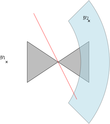
    Let us illustrate the fact that the connectedness of $K$ is not sufficient (i.e. why we require that it is impossible to disconnect the support $K$ of $\mu$ by removing a finite number of points). Consider the case where $K$ is made of the two 2-dimensional simplices embedded in $\mathbb{R}^{2}$, and displayed in grey in Figure 1. We assume that $\mu$ is the restriction of the Lebesgue measure to $K$ and that $Y=\{y_{1},y_{2}\}$. Then, the matrix of the differential of $G$ at $\psi$ is the $2$-by-$2$ matrix given by

    $$\mathrm{D}G(\psi)=\begin{pmatrix}a&-a\\ -a&a\end{pmatrix}\hbox{ where }a=\frac{1}{2\left\|y_{1}-y_{2}\right\|}\mathcal{H}^{1}(\operatorname{Lag}_{1,2}(\psi)\cap K).$$

    If we fix $y_{1}\in\mathbb{R}^{2}$, it is easy to see that for any $y_{2}$ in the blue domain, there exists weights $\psi_{1}$ and $\psi_{2}$ such that the interface $\operatorname{Lag}_{1,2}(\psi)$ (in red) passes through the common vertex between the two simplices, thus implying that $a=0$, hence $\mathrm{D}G(\psi)=0$. In such setting, $G$ is not strictly monotone, the conclusion of Theorem 18 does not hold.

    The end of this section is devoted to the proof of Theorem 18.

    4.1. Preliminary lemmas

    With a slight abuse, we call tangent space to a convex set $K$ the linear space $\mathrm{vect}(K-x)$ for some $x$ in $K$ (this space is independent of the choice of $x$). We denote $\mathrm{relint}(K)$ the relative interior of a convex set $K\subseteq\mathbb{R}^{d}$ and we call dimension of $K$ the dimension of the affine space spanned by $K$.

    Lemma 20.

    Let $e,f$ be convex sets and $E$ and $F$ their tangent spaces. Assume that $\mathrm{relint}(f)\cap\mathrm{relint}(e)\neq\emptyset$. Then,

    $$\dim(e\cap f)=\dim(E\cap F).$$
    Proof.

    Let $G$ be the tangent space to $e\cap f$, so that $\dim(e\cap f)=\dim(G)$. It suffices to show that $G=E\cap F$ to prove that $\dim(e\cap f)=\dim(E\cap F)$. The inclusion $G\subseteq E\cap F$ holds without hypothesis (a tangent vector to $e\cap f$ is always both a tangent vector to $e$ and to $f$). For the reciprocal inclusion, consider $x\in\mathrm{relint}(e)\cap\mathrm{relint}(f)$ and $v\in E\cap F$. Then, by definition of the relative interior, for $t$ small enough one has $x+tv\in e$ and $x+tv\in f$, i.e. $x+tv\in e\cap f$, so that $tv$ belongs to $G$. This shows $G\subseteq E\cap F$ and concludes the proof. ∎

    Lemma 21.

    Let $f\subseteq f^{\prime}$ and $e$ be three convex sets of $\mathbb{R}^{d}$, and $F\subseteq F^{\prime}$ and $E$ be their tangent spaces. Assume that

    • $\mathrm{relint}(f)\cap\mathrm{relint}(e)\neq\emptyset$ ;

    • $\dim(F^{\prime})=\dim(F)+1$ and $\dim(E\cap F^{\prime})=\dim(E\cap F)+1$.

    Then $\dim(e\cap f^{\prime})=\dim(e\cap f)+1$.

    Proof.

    Let us first show that $\mathrm{relint}(e)\cap\mathrm{relint}(f^{\prime})\neq\emptyset$ .We consider a basis $e_{1},\ldots,e_{n}$ of $F$ and a vector $e_{n+1}\in E\cap F^{\prime}$ such that $E\cap F^{\prime}=(E\cap F)\oplus\mathbb{R}e_{n+1}$ and $F^{\prime}=F\oplus\mathbb{R}e_{n+1}$. Let $x_{0}$ be a point in the intersection $\mathrm{relint}(f)\cap\mathrm{relint}(e)$, which we assumed non-empty. There exists $\varepsilon>0$ such that $\Delta:=\mathrm{conv}(\{x_{0}\pm\epsilon e_{i}\mid 1\leqslant i\leqslant n\})\subseteq f.$ Using the assumption that $F^{\prime}$ is the tangent space to $f^{\prime}$, we know that there exists a point $y\in f^{\prime}$ such that $v=y-x_{0}\in F^{\prime}\setminus F$. Consider the convex sets $\Delta_{\pm}$ spanned by $\Delta$ and one of the points $x_{0}\pm v$, $\Delta_{\pm}=\mathrm{conv}(\Delta\cup\{x_{0}\pm v\})$ . The convex set $\Delta_{+}\cup\Delta_{-}$ is a neighborhood of $x_{0}$, meaning that there exists $t\neq 0$ such that $x_{\pm}:=x_{0}\pm te_{n+1}\in\mathrm{relint}(\Delta_{\pm})$. Assume for instance $x_{+}\in\mathrm{relint}(\Delta_{+})\subseteq f^{\prime}$. Since $\Delta_{+}$ has the same dimension as $f^{\prime}$, one has $x_{+}\in\mathrm{relint}(\Delta_{+})\subseteq\mathrm{relint}(f^{\prime})$ and by a standard property of the relative interior one has $(x_{0},x_{+}]=(x_{0},x_{0}+te_{n+1}]\subseteq\mathrm{relint}(f^{\prime})$. Finally, since $x_{0}$ belongs to the relative interior of $e$ and $e_{n+1}\in E$, the segment $(x_{0},x_{0}+te_{n+1}]$ must intersect the relative interior of $e$, proving that $\mathrm{relint}(e)\cap\mathrm{relint}(f^{\prime})\neq\emptyset$.

    Then using Lemma 20, we have $\dim(e\cap f)=\dim(E\cap F)$ and $\dim(e\cap f^{\prime})=\dim(E\cap F^{\prime})=\dim(e\cap f)+1$. ∎

    4.2. Proof of the strict motonicity of $G$

    This theorem will follow using standard arguments, once one has established the connectedness of the graph induced by the Jacobian matrix. Let $\psi\in K^{+}$, $H:=\mathrm{D}G(\psi)$ and consider the graph $\mathcal{G}$ supported on the set of vertices $V=\{1,\ldots,N\}$ and with edges

    $$E(\mathcal{G}):=\{(i,j)\in V^{2}\mid i\neq j\hbox{ and }H_{i,j}(\psi)>0\}.$$
    Lemma 22.

    If $\operatorname{Lag}_{i,j}(\psi)$ intersects some $k$-dimensional simplex $\sigma\in\Sigma$, then the intersection is either a singleton or has dimension $k-1$.

    Proof.

    Denote $\sigma=[x_{0},\ldots,x_{k}]$ and assume that $m=\dim(\operatorname{Lag}_{i,j}(\psi)\cap\sigma)\geqslant 1$. Consider a $p$-dimensional facet $f=[x_{j_{0}},\ldots,x_{j_{p}}]$ of $\sigma$ and a facet $\operatorname{Lag}_{i_{0},\ldots,i_{\ell}}(\psi)=\bigcap_{k=0}^{\ell}\operatorname{Lag}_{i_{k}}(\psi)$ of $\operatorname{Lag}_{i,j}(\psi)$ (we take $i_{0}=i$ and $i_{1}=j$) such that $\dim(\operatorname{Lag}_{i_{0},\ldots,i_{\ell}}(\psi)\cap f)=m$ and assume that both facets are minimal for the inclusion. It is easy to see that this minimality property implies that the relative interiors of $f$ and $\operatorname{Lag}_{i_{0},\ldots,i_{\ell}}(\psi)$ must intersect each other. With Lemma 20, this ensures that

    (4.12) $\displaystyle m$ $\displaystyle=\dim(\operatorname{Lag}_{i_{0},\ldots,i_{\ell}}(\psi)\cap f)$
    (4.13) $\displaystyle=\dim(\{y_{i_{1}}-y_{i_{0}},\ldots,y_{i_{\ell}}-y_{i_{0}}\}^{\perp}\cap\mathrm{vect}(x_{j_{1}}-x_{j_{0}},\ldots,x_{j_{p}}-x_{j_{0}}))=p-\ell,$

    where we used the genericity property (Def 8) to get the last equality. We now prove that $p=k$ and $\ell=1$ by contraction. If we assume that $p<k$, there exists $j_{p+1}\in\{1,\ldots,k\}$ distinct from $\{{j_{0}},\ldots,{j_{p}}\}$. Set $e=\operatorname{Lag}_{i_{0}\ldots,i_{\ell}}(\psi)$, $f=[x_{j_{0}},\ldots,x_{j_{p}}]$ and $f^{\prime}=[x_{j_{0}},\ldots,x_{j_{p+1}}]$. The genericity hypothesis allows us to apply Lemma 21. The conclusion of the lemma is that $\dim(\operatorname{Lag}_{i_{0},\ldots,i_{\ell}}(\psi)\cap f^{\prime})=p+1-\ell>m$, which violates the definition of $m$. By contradiction one must have $p=k$. With the same arguments (removing a point $y_{i_{n}}$ for some $n\in\{0,\ldots,\ell\}$ different from $y_{i}$ and $y_{j}$ from the list if $i_{\ell}\geqslant 1$) we can see that necessarily $\ell=1$. With (4.12) we get $m=k-1$, thus concluding the proof of the lemma. ∎

    Lemma 23.

    The graph $\mathcal{G}$ is connected.

    Proof.

    Consider the finite set

    $$S:=\{x\in\mathbb{R}^{d}\mid\exists\sigma\in\Sigma,\exists i\neq j\in\{1,\ldots,N\},~{}\operatorname{Lag}_{i,j}(\psi)\cap\sigma=\{x\}\}.$$

    For any simplex $\sigma\in\Sigma$, denote $\sigma^{*}=\sigma\setminus S$, and let $K^{*}=K\setminus S$. By definition of a regular simplicial measure (Def. 5), we know that $K^{*}$ is connected. Let $C=\{i_{1},\ldots,i_{c}\}$ be a connected component of the graph $\mathcal{G}$, and define $L=\bigcup_{i\in C}\operatorname{Lag}_{i}(\psi)$ and $L^{\prime}=\bigcup_{i\not\in C}\operatorname{Lag}_{i}(\psi)$.

    Step 1 We first show that for any simplex $\sigma\in\Sigma$, one must have either $\sigma^{*}\subset\mathrm{int}(L)$ or $\sigma^{*}\subset\mathrm{int}(\mathbb{R}^{d}\setminus L)$. For this, it suffices to prove that for any $\sigma\in\Sigma$, $\sigma^{*}\cap\partial{L}=\emptyset$. We argue by contradiction, assuming the existence of a point $x\in\partial{L}\cap\sigma^{*}$. Then, by definition of $\partial L$, there exists $i\in C$ and $j\not\in C$ such that $x\in\operatorname{Lag}_{i,j}(\psi)$. Since $x\in\sigma^{*}$, we know that $x$ does not belong to $S$. This implies that $\operatorname{Lag}_{i,j}(\psi)\cap\sigma$ cannot be a singleton. By the previous Lemma, this gives $\dim(\sigma\cap\operatorname{Lag}_{i,j}(\psi))=d_{\sigma}-1$ so that

    $$H_{ij}(\psi)=\mathrm{const}(y_{i},y_{j})\int_{\sigma\cap\operatorname{Lag}_{i,j}(\psi)}\rho_{\sigma}(x)\mathrm{d}\mathcal{H}^{d_{\sigma}-1}(x)>0.$$

    This shows that $i$ and $j$ are in fact adjacent in the graph $\mathcal{G}$ and contradicts $j\not\in C$.

    Step 2 We now prove that $C$ is equal to $\{1,\ldots,N\}$ by contradiction. We group the simplices $\sigma\in\Sigma$ according to whether $\sigma^{*}$ belongs to $\mathrm{int}(L)$ or to $\mathrm{int}(\mathbb{R}^{d}\setminus L)$. The sets $K^{*}_{i}$ are open for the topology induced on $K^{*}$ because $K^{*}_{1}=\mathrm{int}(L)\cap K^{*}$ and $K^{*}_{2}=\mathrm{int}(L^{\prime})\cap K^{*}$. Since they are also non empty, this violates the connectedness of $K^{*}$. We can conclude that $C=\{1,\ldots,N\}$, i.e. $\mathcal{G}$ is connected. ∎

    Proof of Theorem 18.

    First note that the matrix $H$ is symmetric and therefore diagonalizable in an orthonormal basis. Gershgorin’s circle theorem immediately implies that the eigenvalues of the matrix are negative. The theorem will be established if we are able to show that the nullspace of $H$ (i.e. the eigenspace corresponding to the eigenvalue zero) is the $1$-dimensional space generated by constant functions. The computations presented here are similar to the ones in [4, Lemma 3.3].Consider $v$ in the nullspace and let $i_{0}$ be an index where $v$ attains its maximum, i.e. $i_{0}\in\operatorname{argmax}_{1\leqslant i\leqslant n}v_{i}$. Then, using $Hv=0,$

    $\displaystyle 0=(Hv)_{i_{0}}=H_{i_{0},i_{0}}v_{i_{0}}+\sum_{i\neq i_{0}}H_{i,i_{0}}v_{i}$ $\displaystyle\leqslant H_{i_{0},i_{0}}v_{i_{0}}+\sum_{i\neq i_{0}}H_{i,i_{0}}v_{i_{0}}$
    $\displaystyle=H_{i_{0},i_{0}}v_{i_{0}}+\left(\sum_{i\neq i_{0}}H_{i,i_{0}}\right)v_{i_{0}}=0.$

    The inequality follows from $v_{i}\leqslant v_{i_{0}}$ and from $H_{i,i_{0}}\geqslant 0$, while the third equality comes from $H_{i_{0},i_{0}}=-\sum_{i\neq i_{0}}H_{i_{0},i}.$ This allows us to write $v_{i_{0}}$ as convex combination of values $v_{i}\leqslant v_{i_{0}},$

    $$v_{i_{0}}=\sum_{i\neq i_{0}}\frac{H_{i,i_{0}}}{\sum_{j\neq i_{0}}H_{j,i_{0}}}v_{i}.$$

    This means that for all vertex $i$ adjacent to $i_{0}$ in the graph $\mathcal{G}$ (so that $H_{i,i_{0}}\neq 0$), one must have $v_{i}=v_{i_{0}}$. In particular, the function $v$ also attains its maximum at $i$. By induction and using the connectedness of the graph $\mathcal{G}$, this shows that $v$ has to be constant, i.e. $\operatorname{Ker}(H)=\mathrm{vect}(\{\mathrm{cst}\})$. ∎

    5. Convergence analysis

    In this section, we show the convergence of a damped Newton algorithm for a general function $G:\mathbb{R}^{N}\to\mathbb{R}^{N}$ that satisfies some regularity and strict monotonicity conditions. As a direct consequence, using the results of Sections 3 and 4, we show the convergence with a linear speed of the damped Newton algorithm to solve the non-linear equation (DMA). We denote by $\mathcal{P}_{N}$ the set of $\nu=(\nu_{1},\cdots,\nu_{N})\in\mathbb{R}^{N}$ that satisfies $\nu_{i}\geqslant 0$ and $\sum_{i}\nu_{i}=1$. For a given function $G:\mathbb{R}^{N}\to\mathcal{P}_{N}$ and $\varepsilon>0$, we define the set

    $$\mathcal{K}^{\epsilon}:=\left\{\psi\in\mathbb{R}^{N}\mid\forall i,~{}G_{i}(\psi)\geqslant\epsilon\right\},$$

    where $G(\psi)=(G_{i}(\psi))_{1\leqslant i\leqslant N}$. We then have the following proposition, which is an adaptation to our setting of Theorem 1.5 in [9] and Proposition 2.10 in [14].

    Proposition 24.

    Let $G:\mathbb{R}^{N}\to\mathcal{P}_{N}$ be a function which is invariant under the addition of a constant, i.e. a multiple of $(1,\ldots,1)\in\mathbb{R}^{N}$, and $\varepsilon>0$. We assume the following properties:

    1. (1)

      (Compactness) For every $a\in\mathbb{R}$, the following set is compact:

      $$\mathcal{K}^{\epsilon}_{a}:=\mathcal{K}^{\epsilon}\cap\left\{\psi\in\mathbb{R}^{N}\mid\sum_{i=1}^{N}\psi_{i}=a\right\}=\left\{\psi\in\mathbb{R}^{N}\mid\forall i,~{}G_{i}(\psi)\geqslant\epsilon\mbox{ and }\sum_{i=1}^{N}\psi_{i}=a\right\}.$$
    2. (2)

      ($\mathcal{C}^{1}$ regularity) The function $G$ is of class $\mathcal{C}^{1}$ on $\mathcal{K}^{\epsilon}$.

    3. (3)

      (Strict monotonicity) We have:

      $$\forall\psi\in\mathcal{K}^{\epsilon},~{}\forall v\in\{\mathrm{cst}\}^{\perp}\setminus\{0\},~{}\langle DG(\psi)v\mid v\rangle<0$$

    Then Algorithm 1 converges with linear speed. More precisely, if $\nu\in\mathcal{P}_{N}$ and $\psi_{0}\in\mathbb{R}^{N}$ are such that $\epsilon_{0}=\frac{1}{2}\min\left(\min_{i}G_{i}(\psi_{0}),\min_{i}\nu_{i}\right)>0$, then the iterates $(\psi^{k})$ of Algorithm 1 satisfy the following inequality, where $\tau^{*}\in(0,1]$ depends on $\epsilon_{0}$:

    $$\left\|G(\psi^{k+1})-\nu\right\|\leqslant\left(1-\frac{\tau^{\star}}{2}\right)\left\|G(\psi^{k})-\nu\right\|,$$
    Proof.

    Let $\nu\in\mathcal{P}_{N}$ and $\psi^{0}\in\mathbb{R}^{N}$ such that $\epsilon=\frac{1}{2}\min\left(\min_{i}G_{i}(\psi^{0}),\min_{i}\nu_{i}\right)$ is positive. We put $a=\sum_{i=1}^{N}\psi^{0}_{i}$. Since $\mathcal{K}^{\epsilon}_{a}$ is a compact set, the continuous map $\mathrm{D}G$ is uniformly continuous on $\mathcal{K}^{\epsilon}_{a}$, i.e. there exists a function $\omega:\mathbb{R}^{+}\to\mathbb{R}^{+}$ that satisfies $\lim\limits_{x\to 0}\omega(x)=\omega(0)=0$ and such that

    $$\forall\psi,\tilde{\psi}\in\mathcal{K}^{\epsilon}_{a},~{}\left\|DG(\psi)-DG(\tilde{\psi})\right\|\leqslant\omega(\left\|\psi-\tilde{\psi}\right\|).$$

    Note also that the modulus of continuity $\omega$ can be assumed to be an increasing function. For any $\psi\in\mathcal{K}^{\epsilon}_{a}$, we let $v=DG^{+}(\psi)(G(\psi)-\nu)$ and $\psi_{\tau}=\psi-\tau v$ for any $\tau\geqslant 0$. Since $G$ is of class $\mathcal{C}^{1}$, a Taylor expansion in $\tau$ gives

    (5.14) $$G(\psi_{\tau})=G(\psi-\tau DG^{+}(\psi)(G(\psi)-\nu))=(1-\tau)G(\psi)+\tau\nu+R(\tau)$$

    where $R(\tau)=\int_{0}^{\tau}(DG(\psi_{\sigma})-DG(\psi))vd\sigma$ is the integral remainder. Then, we can bound the norm of $R(\tau)$

    $\displaystyle\left\|R(\tau)\right\|$ $\displaystyle=\left\|\int_{0}^{\tau}(DG(\psi_{\sigma})-DG(\psi))vd\sigma\right\|$
    $\displaystyle\leqslant\left\|v\right\|\int_{0}^{\tau}\omega(\left\|\psi_{\sigma}-\psi\right\|)d\sigma=\left\|v\right\|\int_{0}^{\tau}\omega(\sigma\left\|v\right\|)d\sigma$
    $\displaystyle\leqslant\tau\left\|v\right\|\omega(\tau\left\|v\right\|)$

    where we have used the fact that $\omega$ is an increasing function.

    Step 1 We first want to show that for every $\psi\in\mathcal{K}^{\epsilon}_{a}$ there exists $\tau(\psi)>0$ such that

    (5.15) $$\forall\tau\in(0,\tau(\psi))\quad\quad\psi_{\tau}\in\mathcal{K}^{\epsilon}_{a}\quad\mbox{and}\quad\left\|G(\psi_{\tau})-\nu\right\|\leqslant\left(1-\frac{\tau}{2}\right)\left\|G(\psi)-\nu\right\|.$$

    Recall that for every $i\in\{1,\ldots,N\}$ one has $\nu_{i}\geqslant 2\epsilon$ and $G_{i}(\psi)\geqslant\epsilon$. Thus one gets

    $$G_{i}(\psi_{\tau})\geqslant(1-\tau)G_{i}(\psi)+\tau\nu_{i}+R_{i}(\tau)\geqslant(1+\tau)\epsilon-\left\|R(\tau)\right\|.$$

    So if we choose $\tau$ such that $\left\|R(\tau)\right\|\leqslant\tau\epsilon$ then $G_{i}(\psi_{\tau})\geqslant\epsilon$ and $\psi_{\tau}\in\mathcal{K}^{\epsilon}$. Now, since $\lim\limits_{x\to 0}\omega(x)=0$, there exists $\alpha_{1}>0$ such that for every $0\leqslant\sigma\leqslant\alpha_{1}$, one has $\omega(\sigma)\leqslant\epsilon/\left\|v\right\|$. This implies that if $\tau\leqslant\alpha_{1}/\left\|v\right\|$, then $\left\|R(\tau)\right\|\leqslant\tau\epsilon$ and consequently $\psi_{\tau}\in\mathcal{K}^{\epsilon}$. Note that $G(\psi)-\nu$ belongs to $\{\mathrm{cst}\}^{\perp}$ and that $DG(\psi)$ is an isomorphism from $\{\mathrm{cst}\}^{\perp}$ to $\{\mathrm{cst}\}^{\perp}$. We deduce that $\psi_{\tau}-\psi=\tau v$ belongs to $\{\mathrm{cst}\}^{\perp}$, hence $\psi_{\tau}\in\mathcal{K}^{\epsilon}_{a}$.

    From Eq. (5.14), we have $G(\psi_{\tau})-\nu=(1-\tau)(G(\psi)-\nu)+R(\tau)$. So, to get the second condition of Equation (5.15), it is sufficient to show that $\left\|R(\tau)\right\|\leqslant(\tau/2)\left\|G(\psi)-\nu\right\|$. The estimation on $\left\|R(\tau)\right\|$ and the definition of $v$ gives us

    $$\left\|R(\tau)\right\|\leqslant\tau\left\|DG^{+}(\psi)\right\|\left\|G(\psi)-\nu\right\|\omega(\tau\left\|v\right\|).$$

    Still from the continuity of $\omega$ at 00, we can find $\alpha_{2}>0$ such that for every $\tau\leqslant\alpha_{2}/\left\|v\right\|$ one has $\omega(\tau\left\|v\right\|)\leqslant\epsilon/2\left\|DG^{+}(\psi)\right\|$, thus $\left\|R(\tau)\right\|\leqslant(\tau/2)\left\|G(\psi)-\nu\right\|$. Therefore, by putting $\tau(\psi):=\min(\alpha_{1}/\left\|v(\psi)\right\|,\alpha_{2}/\left\|v(\psi)\right\|,1)$, Equation (5.15) is proved. Note that we impose $\tau(\psi)$ to be less than $1$.

    Step 2 The function $G$ is of class $\mathcal{C}^{1}$ on $\mathcal{K}^{\epsilon}_{a}$. For every $\psi$ in $\mathcal{K}^{\epsilon}_{a}$, $DG(\psi)$ is an isomorphism from $\{\mathrm{cst}\}^{\perp}$ to $\{\mathrm{cst}\}^{\perp}$ and its inverse $DG^{+}(\psi)$ depends continuously on $\psi$. Since $\sum_{i}G_{i}(\psi)=\sum_{i}\nu_{i}$, $G(\psi)-\nu$ belongs to $\{\mathrm{cst}\}^{\perp}$, so the function $v(\psi)=DG^{+}(\psi)(G(\psi)-\nu)$ is also continuous by composition. If $G(\psi)\neq\nu$, the strict monotonicity of $G$ ensures that $v(\psi)\neq 0$ and so $\tau(\psi)=\min(\alpha_{1}/\left\|v(\psi)\right\|,\alpha_{2}/\left\|v(\psi)\right\|,1)$ is also continuous in $\psi$. If $G(\psi)=\nu$, then $v(\psi)=0$. However, by continuity of $v$, the function $\tilde{\psi}\mapsto\tau(\tilde{\psi})$ is constant equal to $1$ in a neighborhood of $\psi$. Hence the function $\psi\mapsto\tau(\psi)$ is globally continuous. Therefore, the infimum of $\tau(\psi)$ over the compact set $\mathcal{K}^{\epsilon}_{a}$ is attained at a point of $\mathcal{K}^{\epsilon}_{a}$, thus is strictly positive. We deduce that we can take a uniform bound $\tau(\psi)=:\tau^{*}>0$ in Equation (5.15) that does not depend on $\psi$. This directly implies the convergence of the damped Newton algorithm with linear speed. ∎

    Proof of Theorem 7.

    The function $G$ appearing in (DMA) satisfies the regularity condition (Theorem 14) and the monotonicity condition (Theorem 18) needed in Proposition 24. It remains to show the compactness condition. Let us take $a\in\mathbb{R}$ and let us show that $\mathcal{K}_{a}^{\epsilon}$ is compact. It is easy to see that $\mathcal{K}_{a}^{\epsilon}$ is closed since $G$ is continuous. Let $\psi\in\mathcal{K}_{a}^{\epsilon}$, $i\neq j$ and $x\in\operatorname{Lag}_{i}(\psi)$. Then one has

    $$\psi_{i}\leqslant\psi_{j}+\left\|x-y_{j}\right\|^{2}-\left\|x-y_{i}\right\|^{2}\leqslant\psi_{j}+\operatorname{diam}(K\cup Y)^{2},$$

    where $\operatorname{diam}(K\cup Y)$ is the diameter of $K\cup Y$. So the differences $|\psi_{i}-\psi_{j}|$ are bounded by $\operatorname{diam}(K\cup Y)^{2}$. Combined with the fact that $\sum_{i}\psi_{i}$ is constant, one has that $\psi$ is bounded by a constant independent on $\psi$. Thus, $K_{a}^{\epsilon}$ is compact. ∎

    6. Numerical results

    In this section, we solve the optimal transport problem in $\mathbb{R}^{3}$ between triangulated surfaces (possibly with holes, with or without a boundary) and point clouds, for the quadratic cost and show it can be used in different settings: optimal quantization of a probability density over a surface, remeshing and point set registration on a mesh. The source density is assumed to be affine on each triangle of the triangulated surface. One crucial aspect of the algorithm is the exact computation of the combinatorics of the Laguerre cells, i.e. the intersection between a triangulated surface and a 3D power diagram, see Equation (2.3). Another important aspect is the initialization step in Algorithm 1, i.e. finding a set of weights $\psi^{0}$ which guarantees that all the initial Laguerre cells have a positive mass. We first explain the algorithm to compute the Laguerre cells, describe how we take the initial weights, before presenting some results.

    6.1. Implementation

    We describe here briefly an algorithm to compute the combinatorics of the intersection of a Power diagram $\operatorname{Pow}:=(\operatorname{Pow}_{i})_{i}$ with a triangulated surface $K=\cup_{\sigma\in\Sigma}\sigma$, with triangles $\sigma\in\Sigma$. Note that in general the intersection of a power cell with $K$ is not convex and can even have several connected components (as illustrated for instance in Figure 2, in the second and third rows). We encode here the triangulated surface $K$ with a connected graph $G_{1}$ where $G_{1}$ is the $1$-skeleton of $K$ (seen as a subset of $\mathbb{R}^{3}$). Similarly, the intersection of the 2D faces of the power diagram with the triangulated surface $K$, namely $G_{2}=\cup_{i}(K\cap\partial\operatorname{Pow}_{i})$, is also encoded by a graph. Let us remark that $G_{2}$ can be disconnected. More precisely, one proceeds as follows:

    1. (1)

      We first split the edges in the graph $G_{1}$ at points in $G_{1}\cap G_{2}$. Since $G_{1}$ is connected, this can be done by a simple traversal, in which we need to intersect the edges of the triangulation with the 2-dimensional power cells.

    2. (2)

      We then traverse $G_{2}$ starting from vertices in $G_{1}\cap G_{2}$ by intersecting the 2-dimensional power-cells with triangles. $G_{2}$ might be disconnected, but we can discover the connected components using the non-visited vertices in $G_{1}\cap G_{2}$. This step provides us with both the geometry and connectivity of $G_{1}\cup G_{2}$, and also an orientation coming from the underlying triangulated surface $K$.

    3. (3)

      The graph $G_{1}\cup G_{2}$ is embedded on the triangulated surface $K$, and the connected components of $K\setminus(G_{1}\cup G_{2})$ are (open) convex polygons. Each of these polygons represents an intersection of the form $\operatorname{Pow}_{i}\cap\sigma$. The boundary of these polygons can easily be reconstructed from $G_{1}\cup G_{2}$ and the orientation (obtained in the second step).

    The main predicates needed here are the intersection tests between a 2D face and a segment and between a power edge (1D face) and a triangle. These predicates can easily be implemented in an exact manner using, for example, the filtered predicates mechanism provided by the CGAL library [17].

    Numerical integration. The computation of $G_{i}(\psi)$ requires the evaluation of integrals of the form $\int_{\operatorname{Lag}_{i}(\psi)\cap\sigma}\rho_{\sigma}(x)\mathrm{d}\mathcal{H}^{2}(x)$ where $\rho_{\sigma}:\mathbb{R}^{3}\to\mathbb{R}^{+}$ is an affine density. In order to evaluate these integrals exactly, we use the classical Gaussian quadrature formulae. In our setting, we have that if $t=[a,b,c]$ is a triangle and $\rho:t\to\mathbb{R}$ is affine, then $\int_{t}\rho(x)\mathrm{d}\mathcal{H}^{2}(x)=\operatorname{Area}(t)\cdot\rho((a+b+c)/3)$.

    Choice of the initial weights. The following proposition shows how to choose the initial weights so as to avoid empty Laguerre cells.

    Proposition 25.

    Let $K\subset\mathbb{R}^{d}$ be a compact set, $Y=\{y_{1},\ldots,y_{N}\}\subset\mathbb{R}^{d}$ be a point cloud and $\psi^{0}_{i}=-\mathrm{d}(y_{i},K)^{2}$. Then, all the Laguerre cells $\operatorname{Lag}_{i}(\psi^{0})$ are non-empty:

    $$\emptyset\neq\{x\in K\mid\mathrm{d}(y_{i},K)=\left\|x-y_{i}\right\|\}\subseteq\operatorname{Lag}_{i}(\psi^{0}).$$
    Proof.

    Let $i\in\{1,\ldots,N\}$, and $x\in K$ be such that $d(y_{i},K)=\left\|x-y_{i}\right\|$. Then for $j\in\{1,\ldots,N\}$

    $$\left\|x-y_{j}\right\|^{2}+\psi^{0}_{j}=\left\|x-y_{j}\right\|^{2}-d(y_{j},K)^{2}\geqslant d(y_{j},K)^{2}-d(y_{j},K)^{2}=0=\left\|x-y_{i}\right\|^{2}+\psi^{0}_{i},$$

    meaning that $x\in\operatorname{Lag}_{i}(\psi^{0})$.∎

    In particular, this proposition applies to the case where $K$ is a triangulated surface. Thus, it means that we can find weights such that the initial Laguerre cells are not empty. In practice, if needed, we slightly perturb $\psi^{0}$ to ensure that all the Laguerre cells also have non empty interior, thus have a positive mass.

    6.2. Results and applications

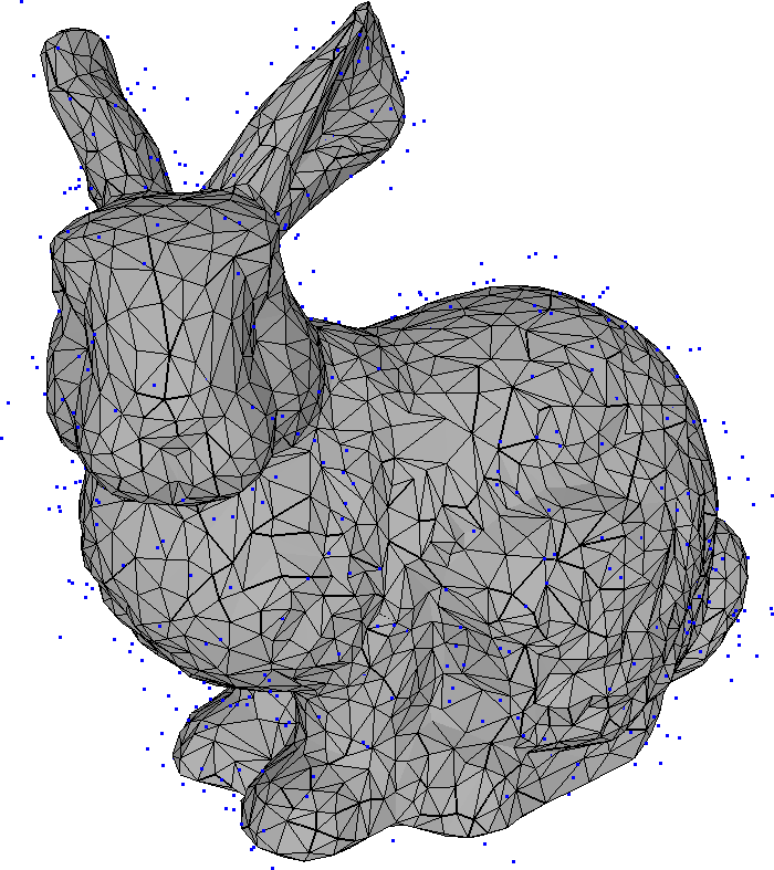
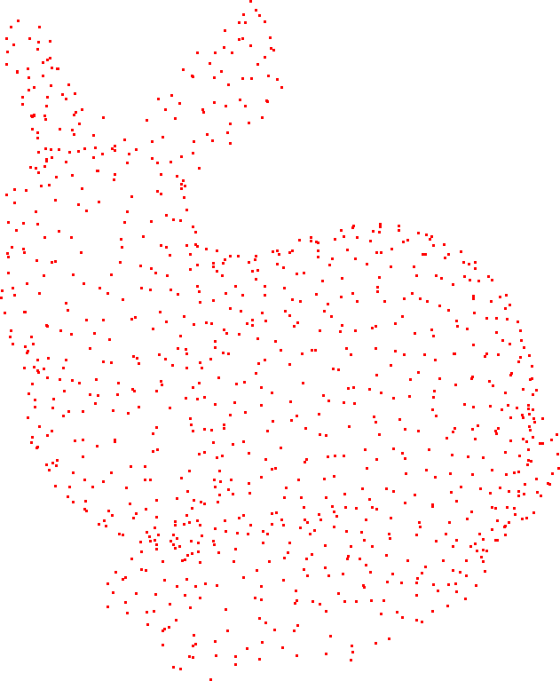
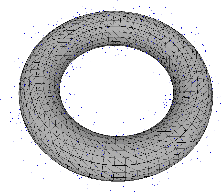
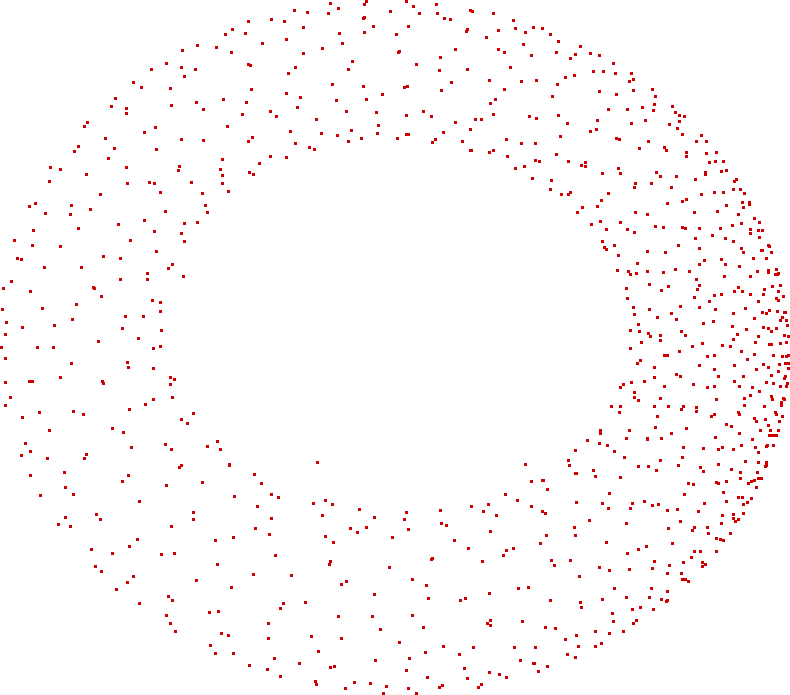
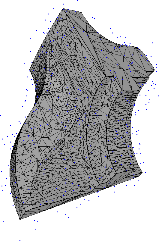
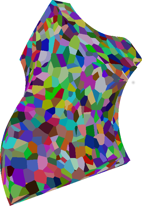
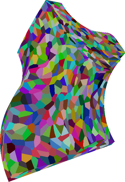
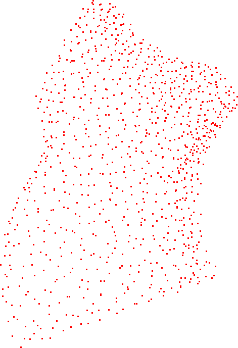
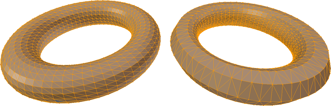
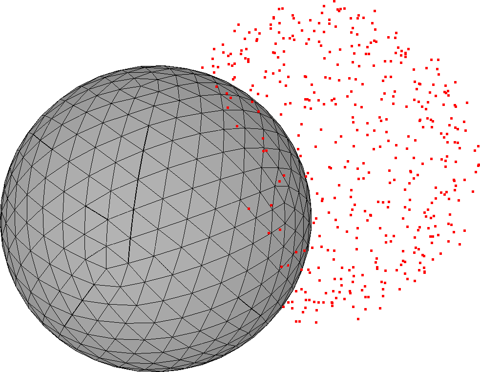
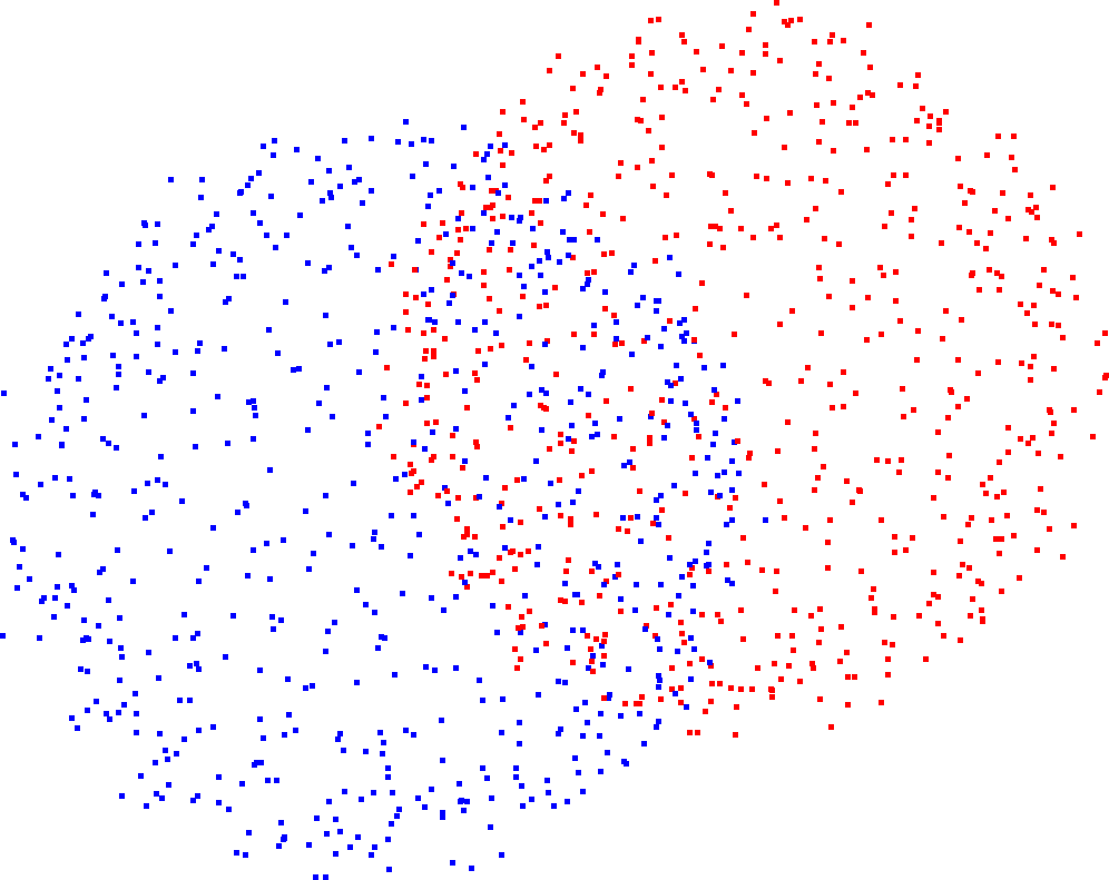
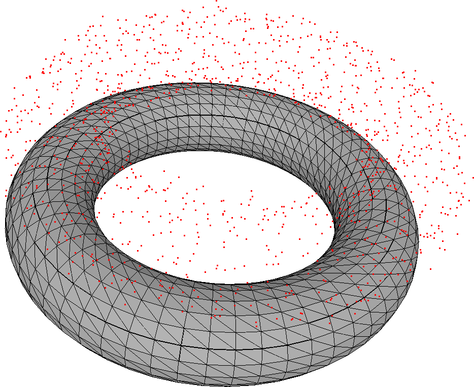
    We compute the optimal transport map between a piecewise linear measure defined on a triangulated surface $K$ and a discrete measure defined on a 3D point cloud. Even if we can handle non uniform measures, in the examples presented here, the source density is uniform over the triangulation: $\rho_{\sigma}=1/\operatorname{Area}(K)$ for every $\sigma\in\Sigma$, where $\operatorname{Area}(K)$ is the area of $K$. The point cloud is chosen to be a noisy version of points sampled on the mesh. In the examples, the solutions are computed up to an error of $\eta=10^{-6}$.

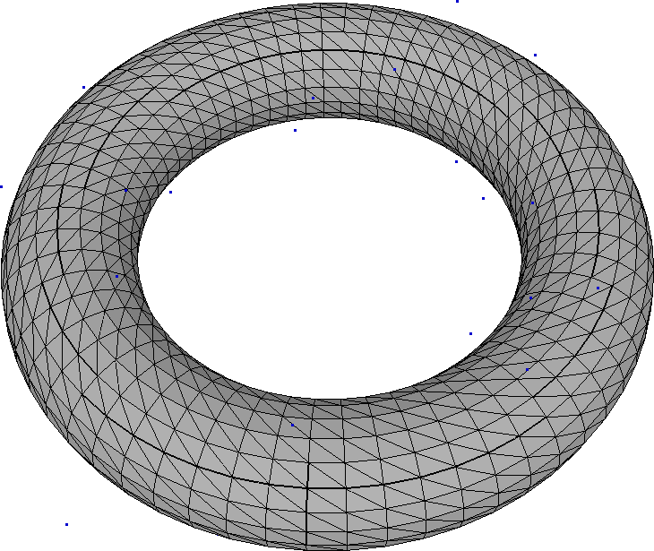
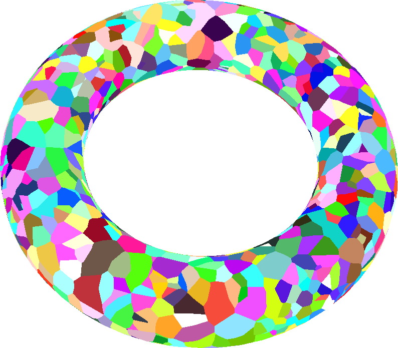
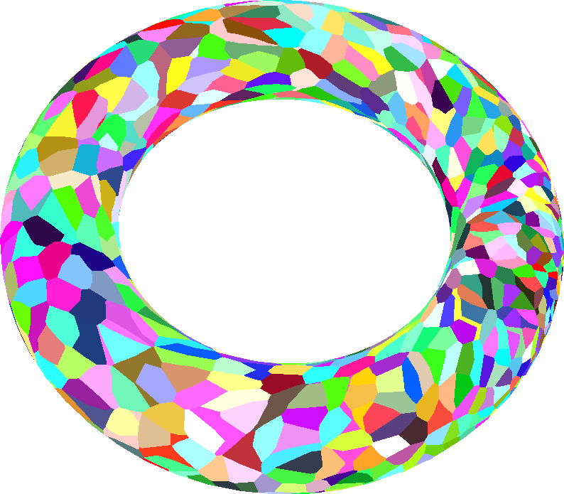
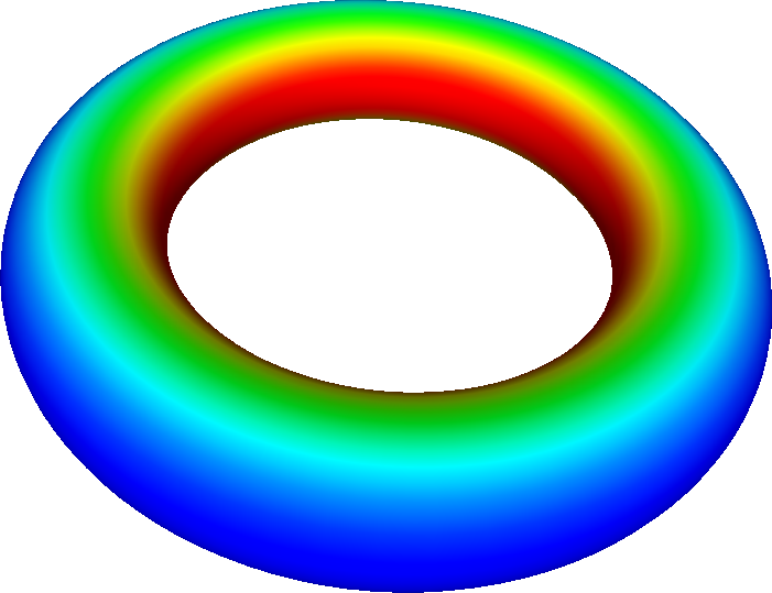
    The first two rows of Figure 2 displays results for a uniform target measure and the last two for a non-uniform one. Remark that in this case the non uniformity creates smaller Laguerre cells on the right side. Note that the centroids of the Laguerre cells provide naturally a correspondence between the point cloud and the triangulated surface: we associate to each $y_{i}$ the centroid of the Laguerre $\operatorname{Lag}_{i}(\psi^{k})$, where $\psi^{k}$ is the output of Algorithm 1. In practice, the number of iterations remains small even for large point sets. For instance, if we choose $10,000$ noisy samples on the torus, the algorithm takes $16$ iterations to solve the problem.

    Remark 26.

    We also underline that the Laguerre cells can be non geodesically convex and even disconnected (as illustrated in the second and third columns of Figure 2) which shows that our method handles more general settings than [9], i.e. cost functions whose Laguerre cells cannot be convex in any chart (violating the hypothesis of [9], Def 1.1).

    Refer to caption
    Refer to caption
    Refer to caption
    Refer to caption
    Refer to caption
    Refer to caption
    Refer to caption
    Refer to caption
    Refer to caption
    Refer to caption
    Refer to caption
    Refer to caption
    Refer to caption
    Refer to caption
    Refer to caption
    Refer to caption
    Figure 2. From left to right: Mesh and initial point cloud (in blue), Initial Laguerre cells, Final Laguerre cells, Centroids of the final Laguerre cells. The source measure is uniform. In the first two rows, the target density is uniform while in the last two, it linearly decreases from left to right. In the first row, $N=50$ while in the other rows, $N=1000$. Computation time (number of iterations): 3s (4) / 41s (7) / 74s (14) / 58s (9).

    We now show how to use this algorithm as a building block for higher level operations: optimal quantization of surfaces, remeshing and point set registration. The goal here is not to compete with state of the art algorithms for these applications but rather to show the applicability of Algorithm 1 in more complex situations.

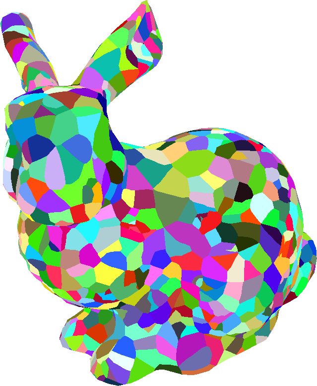
    Optimal quantization of a surface

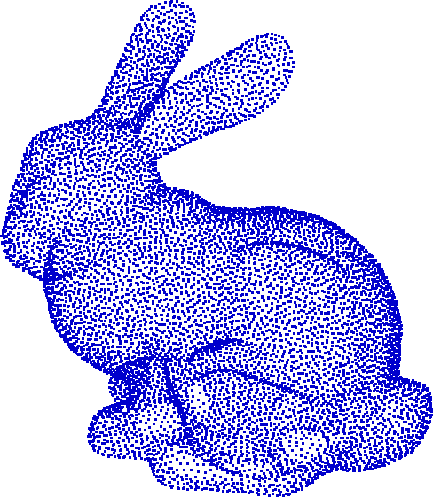
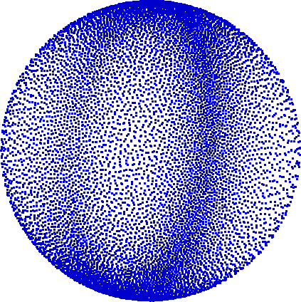
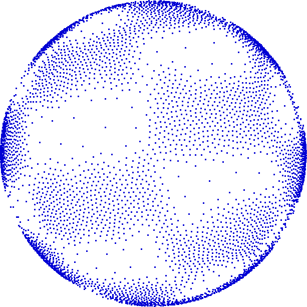
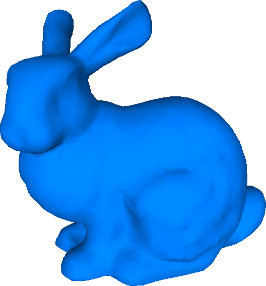
    Optimal quantization is a sampling technique used to approximate a density function with a point cloud, or more accurately a finitely supported measure. It has many applications such as in image dithering or in computer graphics (see [6] for more details). Here, we show how to perform this kind of sampling on triangulated surfaces. Given a triangulated surface $K\subset\mathbb{R}^{3}$ and a density $\mu$ on $K$, we first define $Y_{0}$ as the set of vertices of $K$ and consider the constant probability measure $\nu_{0}$ on $Y_{0}$. For each $k\geq 0$, we solve the optimal transport between $\mu$ on $K$ and $\nu_{k}$ on $Y_{k}$ and pick one point, for instance the centroid, per Laguerre cell. We iterate this procedure by choosing for the new point cloud $Y_{k+1}$ the set of the previously computed centroids and for $\nu_{k+1}$ the uniform measure over $Y_{k+1}$. After a few iterations, this gives us a (locally) optimal quantization of $K$. Figure 3 shows examples of sampling on different surfaces with different densities.

    Refer to caption
    Refer to caption
    Refer to caption
    Refer to caption
    Figure 3. Optimal quantization of triangulated surfaces for different densities and surfaces. From left to right: uniform density $\mu=1$ on the Stanford Bunny (10k points); non-linear density $\mu(x,y,z)=e^{-3|y|}$ on the sphere (10k points); checkerboard texture and sampling for the density corresponding to the UV-mapping of the texture on the hemisphere (5k points).

    Remeshing

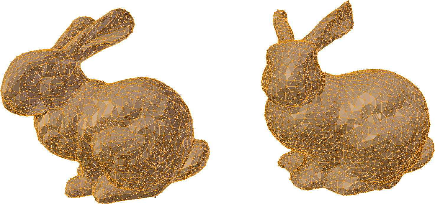
    We now consider the following problem: given a triangulated surface $K$, a density $\mu$ supported on this mesh, we want to build a new mesh such that the distribution of triangles respect this density, meaning that we want more triangles where the density is more important. This has applications for instance in finite element methods for solving partial differential equations where the quality of the discretization matters. To do this, we can use the following simple procedure: we consider the uniform discrete measure $\nu$ supported on the vertices of $K$; we solve the optimal transport between $\mu$ on $K$ and $\nu$; the new mesh will be taken as the dual (in the graph sense) of the final Laguerre diagram. See Figure 4 for two examples for different source densities.

    Refer to caption
    Refer to caption
    Refer to caption
    Refer to caption
    Figure 4. Remeshing using optimal transport. From left to right: source density; initial mesh and remeshed surface. First row: Uniform density: $\mu=1$; Second row: $\mu$ is proportional to a mean curvature estimator of the source mesh. Number of vertices for each model: Bunny: 2.2k; Torus: 5.6k.

    Point set registration

    We finally consider the rigid point set registration to a mesh. Given a triangulated surface $K$ and a point cloud $Y$, we want to find a rigid transformation $T$ such that the $L^{2}$ distance between $K$ and $T(Y)$ is minimal. The most popular method to do this is the Iterative Closest Point (ICP) algorithm developed in [2]. For this algorithm, we need to be able to compute for each point $y_{i}$ from the cloud $Y$ its closest point on the mesh $K$. We can replace the traditional nearest neighbor query with the following routine: we solve the optimal transport between the constant probability measure $\mu$ on $K$ and the constant probability measure $\nu$ on $Y$, then associate each point $y_{i}$ to a point (for instance the centroid) of the Laguerre cell $\operatorname{Lag}_{i}(\psi)$ where $\psi\in\mathbb{R}^{N}$ are the final weights. The resulting algorithm is called Optimal Transport ICP (OT-ICP). See Figure 5 for one example. In our results, OT-ICP converges in much less iterations than standard ICP, namely 3 iterations versus 20 iterations for the same stopping criterion in our two test cases. Despite this, the remains higher with optimal transport. One may hope that the use of optimal transport ”convexifies” the energy optimized by ICP, in the same way the choice of a Wasserstein loss instead of a $\mathrm{L}^{2}$ distance seems to mitigates the cycle-skipping issue in full waveform inversion [7].

    Refer to caption
    Refer to caption
    Refer to caption
    Refer to caption
    Refer to caption
    Refer to caption
    Figure 5. Optimal transport-ICP algorithm. From left to right: initial mesh (in grey) and initial point cloud (in red); initial (red) and final (blue) point clouds using traditional ICP; initial (red) and final (blue) using optimal transport.

    References