Framelet perturbation and application to nouniform sampling approximation for Sobolev space

Abstract.

The Sobolev space $H^{s}(\mathbb{R}^{d})$, where $s>d/2$, is an important function space that has many applications in various areas of research. Attributed to the inertia of a measuring instrument, it is desirable in sampling theory to reconstruct a function by its nonuniform samples. In the present paper, we investigate the problem of constructing the approximation to all the functions in $H^{s}(\mathbb{R}^{d})$ with nonuniform samples by utilizing dual framelet systems for the Sobolev space pair $(H^{s}(\mathbb{R}^{d}),H^{-s}(\mathbb{R}^{d}))$. We first establish the convergence rates of the framelet series in $(H^{s}(\mathbb{R}^{d}),H^{-s}(\mathbb{R}^{d}))$, and then construct the framelet approximation operator holding for the entire space $H^{s}(\mathbb{R}^{d})$. Using the approximation operator, any function in $H^{s}(\mathbb{R}^{d})$ can be approximated at the exponential rate with respect to the scale level. We examine the stability property for the perturbations of the framelet approximation operator with respect to shift parameters, and obtain an estimate bound for the perturbation error. Our result shows that under the condition $s>d/2$, the approximation operator is robust to the shift perturbation. These results are used to establish the nonuniform sampling approximation for every function in $H^{s}(\mathbb{R}^{d})$. In particular, the new nonuniform sampling approximation error is robust to the jittering of the samples.

1. Introduction

Sampling is a fundamental tool for the conversion between an analogue signal and its digital form (A/D). The most classical sampling theory is the Whittaker-Kotelnikov-Shannon (WKS) sampling theorem [30, 31], which states that a bandlimited signal can be perfectly reconstructed if it is sampled at a rate greater than its Nyquist frequency. The WKS sampling theorem holds only for bandlimited signals. In order to extend the sampling theorem to non-bandlimited signals, researchers have established various sampling theorems for many other function spaces. Such examples include the sampling theory for shift-invariant subspaces (c.f. [1, 2, 34, 38, 39]), for reproducing kernel subspaces of $L^{2}(\mathbb{R}^{d})$ (c.f. [13, 34, 35, 36, 8]), and for subspaces from the generalized sinc function (c.f. [9]).

For any $s\in\mathbb{R}$, the Sobolev space $H^{s}(\mathbb{R}^{d})$ is defined as

(1.1) $$H^{s}(\mathbb{R}^{d})=\Big{\{}f:\int_{\mathbb{R}^{d}}|\widehat{f}(\xi)|^{2}(1+||\xi||_{2}^{2})^{s}d\xi<\infty\Big{\}},$$

where $\widehat{f}(\xi):=\int_{\mathbb{R}^{d}}f(x)e^{-ix\cdot\xi}dx$ is the Fourier transform of $f$. When $s>d/2$, the function theory of $H^{s}(\mathbb{R}^{d})$ has been extensively applied to various problems such as the boundedness of the Fourier multiplier operator [6, 12, 20], viscous shallow water system [26, 40], PDE [27], and signal analysis [10, 28]. On the other hand, it will be seen in Theorem 2.4 or Remark 2.2 that the condition $s>d/2$ is necessary to guarantee that the approximation system in $H^{s}(\mathbb{R}^{d})$ is robust to the perturbation of the shift parameters, which is crucial for our construction of nonuniform sampling approximation. Moreover, it is easy to check that many frequently used spaces such as the bandlimited function space, wavelet subspaces [7, 11] and the cardinal B-spline subspaces [7, 14] (in which the generator is continuous) are all contained in $H^{s}(\mathbb{R}^{d})$. Readers are referred to Han and Shen [14] for the Sobolev smoothness of box splines.

Since $H^{s}(\mathbb{R}^{d})$ and $H^{-s}(\mathbb{R}^{d})$ are isometric under a mapping provided in the proof of [14, Proposition 2.1], we can treat $H^{-s}(\mathbb{R}^{d})$ as the dual space of $H^{s}(\mathbb{R}^{d})$. It can be seen in Theorem 3.1 or [23] that by using special dual framelets in $(H^{s}(\mathbb{R}^{d}),H^{-s}(\mathbb{R}^{d}))$, the inner products can expressed directly by the values of functions, which makes the sampling approximation possible. In the one-dimensional $(d=1$) case, a uniform sampling theorem for all the functions in $H^{s}(\mathbb{R})$, where $s>1/2$, was established by Li and Yang in [23]. Attributed to the inertia of a measuring instrument, the samples we acquire may well be jittered and thus nonuniform [32, 33, 35]. Therefore it seems necessary to establish a theory for nonuniform sampling for all the functions in $H^{s}(\mathbb{R^{d}}^{d})$. The purpose of this paper is to build such a theory by using a pair of dual framelet system for the Sobolev space pair $(H^{s}(\mathbb{R}^{d}),H^{-s}(\mathbb{R}^{d}))$ $(s>d/2$).

We first introduce some necessary notations and terminologies for framelets in Sobolev spaces. More details can be found in Han and Shen [14] where the dual framelets for the dual pair $(H^{s}(\mathbb{R}^{d}),H^{-s}(\mathbb{R}^{d}))$ were first introduced. We remark that, comparing with those in $L^{2}(\mathbb{R}^{d})$, the framelet in $H^{s}(\mathbb{R}^{d})$ does not necessarily have vanishing moment. Therefore the construction of the framelet system seems much more easier in this case. Readers are referred to [17, 18] for Han’s continuing work in the distribution spaces.

By (1.1), $H^{s}(\mathbb{R}^{d})$ is equipped with the inner product $\langle\cdot,\cdot\rangle_{H^{s}(\mathbb{R}^{d})}$ defined by

(1.2) $$\langle f,g\rangle_{H^{s}(\mathbb{R}^{d})}=\frac{1}{(2\pi)^{d}}\int_{\mathbb{R}^{d}}\widehat{f}(\xi)\overline{\widehat{g}(\xi)}(1+||\xi||_{2}^{2})^{s}d\xi,\ \ \ \ \forall f,g\in H^{s}(\mathbb{R}^{d}),$$

where $\overline{\widehat{g}}$ is the complex conjugate. The deduced norm $||\cdot||_{H^{s}(\mathbb{R}^{d})}$ of $\langle\cdot,\cdot\rangle_{H^{s}(\mathbb{R}^{d})}$ is naturally given by

$$||f||_{H^{s}(\mathbb{R}^{d})}=\frac{1}{(2\pi)^{d/2}}\Big{(}\int_{\mathbb{R}^{d}}|\widehat{f}(\xi)|^{2}(1+||\xi||_{2}^{2})^{s}d\xi\Big{)}^{1/2}.$$

It is easy to check that the bilinear functional $\langle\cdot,\cdot\rangle:(H^{s}(\mathbb{R}^{d}),H^{-s}(\mathbb{R}^{d}))\longrightarrow\mathbb{C}$ defined by

$$\langle f,g\rangle=\frac{1}{(2\pi)^{d}}\int_{\mathbb{R}^{d}}\widehat{f}(\xi)\overline{\widehat{g}(\xi)}d\xi,\ \forall f\in H^{s}(\mathbb{R}^{d}),g\in H^{-s}(\mathbb{R}^{d})$$

satisfies $|\langle f,g\rangle|\leq||f||_{H^{s}(\mathbb{R}^{d})}||g||_{H^{-s}(\mathbb{R}^{d})}.$ Straightforward observation on (1.1) gives that $H^{s_{1}}(\mathbb{R}^{d})$ $\supseteq H^{s_{2}}(\mathbb{R}^{d})$ if and only if $s_{1}\leq s_{2}$. When $s=0$, we have that $H^{0}(\mathbb{R}^{d})=L^{2}(\mathbb{R}^{d})$, and the corresponding norm $||\cdot||_{H^{0}(\mathbb{R}^{d})}$ is the usuall $L_{2}$-norm $||\cdot||_{2}$. In what follows we will use the same norm denotation $||\cdot||_{2}$ for $L^{2}(\mathbb{R}^{d})$ and the Euclidean space $\mathbb{R}^{d}.$ The two norms can be easily identified from the context. For any $f\in H^{s}(\mathbb{R}^{d})$, define its bracket product $[f,f]_{s}$ as

(1.3) $$[f,f]_{s}(\xi):=\sum_{k\in\mathbb{Z}^{d}}|\widehat{f}(\xi+2k\pi)|^{2}(1+||\xi+2k\pi||_{2}^{2})^{s}.$$

When $f$ is compactly supported, we have that $[f,f]_{s}\in L_{\infty}(\mathbb{R}^{d})$. We refer to Han’s method [15] for more information about the bracket product estimation.

A $d\times d$ integer matrix $M$ is referred to as a dilation matrix if all its eigenvalues are strictly larger than $1$ in modulus. Throughout this paper, we are interested in the case that $M$ is isotropic. Specifically, $M$ is similar to $\mbox{diag}(\lambda_{1},\lambda_{2},\cdots,\lambda_{d})$ with $|\lambda_{k}|=m:=|\det M|^{1/d}$ for $k=1,2,\ldots,d.$ Denote by $\Gamma_{M^{T}}$ the complete set of representatives of distinctive cosets of the quotient group $[(M^{T})^{-1}\mathbb{Z}^{d}]/\mathbb{Z}^{d}.$ Suppose that $\phi\in H^{s}(\mathbb{R}^{d}),s\in\mathbb{R},$ is an $M$-refinable function given by

(1.4) $$\widehat{\phi}(M^{T}\cdot)=\widehat{a}(\cdot)\widehat{\phi}(\cdot),$$

where $\widehat{a}(\cdot):=\sum_{k\in\mathbb{Z}^{d}}a[k]e^{ik\cdot}$ is referred to as the mask symbol of $\phi$, and $\{\psi^{\ell}\}^{L}_{\ell=1}$ is a set of wavelet functions defined by

(1.5) $$\widehat{\psi^{\ell}}(M^{T}\cdot)=\widehat{b^{\ell}}(\cdot)\widehat{\phi}(\cdot),$$

where the $2\pi\mathbb{Z}^{d}$-periodic trigonometric polynomial $\widehat{b^{\ell}}(\cdot)$ is the mask symbol of $\psi^{\ell}$. Now a wavelet system $X^{s}(\phi;$ $\psi^{1},\ldots,\psi^{L})$ in $H^{s}(\mathbb{R}^{d})$ is defined as

(1.8) $$\begin{array}[]{lllll}X^{s}(\phi;\psi^{1},\ldots,\psi^{L})&:=\{\phi_{0,k}:k\in\mathbb{Z}^{d}\}\\ &\quad\cup\{\psi^{\ell,s}_{j,k}:k\in\mathbb{Z}^{d},j\in\mathbb{N}_{0},\ell=1,\ldots,L\},\end{array}$$

where $\phi_{0,k}=\phi(\cdot-k)$, $\psi^{\ell,s}_{j,k}=m^{j(d/2-s)}\psi^{\ell}(M^{j}\cdot-k)$ and $\mathbb{N}_{0}:=\mathbb{N}\cup\{0\}$. If there exist two positive constants $C_{1}$ and $C_{2}$ such that

(1.10) $$\begin{array}[]{lllll}C_{1}||f||_{H^{s}(\mathbb{R}^{d})}^{2}\displaystyle\leq\sum_{k\in\mathbb{Z}^{d}}|\langle f,\phi_{0,k}\rangle_{H^{s}(\mathbb{R}^{d})}|^{2}+\sum^{L}_{\ell=1}\sum_{j\in\mathbb{N}_{0}}\sum_{k\in\mathbb{Z}^{d}}|\langle f,\psi^{\ell,s}_{j,k}\rangle_{H^{s}(\mathbb{R}^{d})}|^{2}\leq C_{2}||f||_{H^{s}(\mathbb{R}^{d})}^{2}\end{array}$$

holds for every $f\in H^{s}(\mathbb{R}^{d}),$ then we say that $X^{s}(\phi;\psi^{1},\ldots,\psi^{L})$ is an $M$-framelet system in $H^{s}(\mathbb{R}^{d})$. If there exists another $M$-framelet system $X^{-s}(\widetilde{\phi};\widetilde{\psi}^{1},\ldots,\widetilde{\psi}^{L})$ in $H^{-s}(\mathbb{R}^{d})$ such that for any $f\in H^{s}(\mathbb{R}^{d})$ and $g\in H^{-s}(\mathbb{R}^{d})$, there holds

(1.11) $$\langle f,g\rangle=\sum_{k\in\mathbb{Z}^{d}}\langle\phi_{0,k},g\rangle\langle f,\widetilde{\phi}_{0,k}\rangle+\sum^{L}_{\ell=1}\sum_{j\in\mathbb{\mathbb{N}}_{0}}\sum_{k\in\mathbb{Z}^{d}}\langle\psi^{\ell,s}_{j,k},g\rangle\langle f,\widetilde{\psi}^{\ell,-s}_{j,k}\rangle,$$

then we say that $X^{s}(\phi;\psi^{1},\ldots,\psi^{L})$ and $X^{-s}(\widetilde{\phi};\widetilde{\psi}^{1},\ldots,\widetilde{\psi}^{L})$ form a pair of dual $M$-framelet systems in $(H^{s}(\mathbb{R}^{d}),H^{-s}(\mathbb{R}^{d}))$. For any function $f\in H^{s}(\mathbb{R}^{d})$, it follows from (1.11) that

(1.13) $$\begin{array}[]{lll}f=\displaystyle\sum_{k\in\mathbb{Z}^{d}}\langle f,\widetilde{\phi}_{0,k}\rangle\phi_{0,k}+\sum^{L}_{\ell=1}\sum_{j\in\mathbb{\mathbb{N}}_{0}}\sum_{k\in\mathbb{Z}^{d}}\langle f,\widetilde{\psi}^{\ell,-s}_{j,k}\rangle\psi^{\ell,s}_{j,k}.\end{array}$$

Our goal is to construct the nonuniform sampling approximation to any function $f\in H^{s}(\mathbb{R}^{d}),$ $s>d/2$. Our approximation will be derived from the truncation form $\mathcal{S}_{\phi}^{N}f$ of the series in (1.13), defined by

(1.14) $$\mathcal{S}_{\phi}^{N}f:=\sum_{k\in\mathbb{Z}^{d}}\langle f,\widetilde{\phi}_{0,k}\rangle\phi_{0,k}+\sum^{L}_{\ell=1}\sum^{N-1}_{j=0}\sum_{k\in\mathbb{Z}^{d}}\langle f,\widetilde{\psi}^{\ell,-s}_{j,k}\rangle\psi^{\ell,s}_{j,k},$$

where $N$ is sufficiently large. The first natural problem is how to estimate the approximation error $||(I-\mathcal{S}_{\phi}^{N})f||$, where $I$ is the identity operator, and $||\cdot||$ is the desired norm. When $f$ belongs to the Schwartz class of functions, the estimate of $||(I-\mathcal{S}_{\phi}^{N})f||_{2}$ was given in [22, Theorem 16]. In [24], the approximation error $||(I-\mathcal{S}_{\phi}^{N})f||_{H^{s}(\mathbb{R}^{d})}$ was estimated when $f$ satisfies

$$|\widehat{f}(\xi)|\leq C(1+||\xi||_{2})^{\frac{-d-\alpha}{2}}\ \hbox{for}\ \hbox{every}\ \xi\in\mathbb{R}^{d},$$

with $\alpha>0$ and a constant $C$ being dependent on $f$. When the framelet system $X^{-s}(\widetilde{\phi};\widetilde{\psi}^{1},\ldots,\widetilde{\psi}^{L})$ belongs to $L^{2}(\mathbb{R}^{d})$, for any $f\in H^{s}(\mathbb{R}^{d})$, the estimate of $||(I-\mathcal{S}_{\phi}^{N})f||_{2}$ was obtained in [19] and [22]. In the present paper, by using a special pair of dual framelet systems $X^{s}(\phi;\psi^{1},\ldots,\psi^{L})$ and $X^{-s}(\widetilde{\phi};\widetilde{\psi}^{1},\ldots,\widetilde{\psi}^{L})$, we aim at constructing the nonuniform sampling approximation to all the functions in $H^{s}(\mathbb{R}^{d})$, where the system $X^{-s}(\widetilde{\phi};\widetilde{\psi}^{1},\ldots,\widetilde{\psi}^{L})$ in $H^{-s}(\mathbb{R}^{d})$ does not actually belong to $L^{2}(\mathbb{R}^{d})$. Therefore in order to construct the sampling approximation in this setting, we need to estimate $||(I-\mathcal{S}_{\phi}^{N})f||$ for any $f\in H^{s}(\mathbb{R}^{d})$, not requiring $X^{-s}(\widetilde{\phi};\widetilde{\psi}^{1},\ldots,\widetilde{\psi}^{L})$ being in $L^{2}(\mathbb{R}^{d})$. Such an estimate will be presented in Theorem 2.2.

It will be seen in (3.6) and (2.38) that the nonuniformity of samples is substantially derived from the perturbation of shifts of the sampling system $\{\Delta^{-s}_{N,k}\}_{k\in\mathbb{Z}^{d}}\subseteq H^{-s}(\mathbb{R}^{d})$, where $\Delta\in H^{-s}(\mathbb{R}^{d})$ is a special refinable function to be defined in (3.4), and $\Delta^{-s}_{N,k}$ will be given via (2.35). Thus, in order to construct the nonuniform sampling approximation, we need to establish the estimate for the perturbation error of $\mathcal{S}_{\phi}^{N}f$ when the shifts of $\{\widetilde{\phi}^{-s}_{N,k}\}_{k\in\mathbb{Z}^{d}}$ are perturbed, where $\widetilde{\phi}$ is any refinable function in $H^{-s}(\mathbb{R}^{d})$. Our second main Theorem 2.6 establishes such an error estimate.

In the Section 3 we present a main application of our two main results. By using a pair of dual framelets for $(H^{s}(\mathbb{R}^{d}),H^{-s}(\mathbb{R}^{d})),$ we are able to construct the nonuniform sampling approximation to any function in $H^{s}(\mathbb{R}^{d})$ where $s>d/2$. We also compare the main results of this paper with the existing ones in the literature, and present two simulation examples to demonstrate the approximation efficiency in numerical experiments.

2. Perturbed framelet approximation system in Sobolev space

In this section we will first estimate the convergence rate of the coefficient sequence $\big{\{}\langle f,\widetilde{\psi}^{\ell,-s}_{j,k}\rangle\big{\}}$ in (1.13). Based on the convergence rate estimation, the approximation error $(I-\mathcal{S}_{\phi}^{N})f$ for any $f\in H^{s}(\mathbb{R}^{d})$ will be estimated, not requiring $X^{-s}(\widetilde{\phi};\widetilde{\psi}^{1},\ldots,\widetilde{\psi}^{L})$ being in $L^{2}(\mathbb{R}^{d})$. Moreover, the corresponding perturbation error of $\mathcal{S}_{\phi}^{N}f$ will be given when the shifts of approximation system $\{\widetilde{\phi}^{-s}_{N,k}\}_{k\in\mathbb{Z}^{d}}$ are perturbed, where $\widetilde{\phi}^{-s}_{N,k}$ will be defined in (2.35).

2.1. Framelet approximation system

For any $\alpha:=(\alpha_{1},\alpha_{2},\ldots,\alpha_{d})\in\mathbb{N}^{d}_{0}$ and $x:=(x_{1},x_{2},\ldots,x_{d})\in\mathbb{R}^{d}$, define $x^{\alpha}=\prod^{d}_{k=1}x^{\alpha_{k}}_{k}$. For any function $f:\mathbb{R}^{d}\longrightarrow\mathbb{C}$, its $\alpha$th partial derivative $\frac{\partial^{\alpha}}{\partial x^{\alpha}}f$ is defined as

$$\frac{\partial^{\alpha}}{\partial x^{\alpha}}f=\frac{\partial_{1}^{\alpha_{1}}\partial_{2}^{\alpha_{2}}\cdots\partial_{d}^{\alpha_{d}}}{\partial x_{1}^{\alpha_{1}}\partial x_{2}^{\alpha_{2}}\cdots\partial x_{d}^{\alpha_{d}}}f.$$

We say that a function $f:\mathbb{R}^{d}\longrightarrow\mathbb{C}$ has $\kappa+1(\in\mathbb{N})$ vanishing moments if

$$\frac{\partial^{\alpha}}{\partial x^{\alpha}}\widehat{f}(0)=0$$

for any $\alpha\in\mathbb{N}^{d}_{0}$ such that $||\alpha||_{1}\leq\kappa$, where $||\cdot||_{1}$ is the $1$-norm of a vector.

In the proof of Theorem 2.2, we will see that the crucial task for estimating $||(I-\mathcal{S}_{\phi}^{N})f||_{H^{s}(\mathbb{R}^{d})}$ is to estimate the convergence rate of the coefficient sequence $\{\langle f,\widetilde{\psi}^{\ell,-s}_{j,k}\rangle\}_{j,k,\ell}$ in (1.13). As such, we first estimate the convergence rate of $\{\langle f,\widetilde{\psi}^{\ell,-s}_{j,k}\rangle\}_{j,k,\ell}$ in Lemma 2.1.

Lemma 2.1.

Let $s>0$ and $\widetilde{\phi}\in H^{-s}(\mathbb{R}^{d})$ be $M$-refinable. Moreover, suppose that $\widetilde{\phi}\in H^{-t}(\mathbb{R}^{d})$ where $0<t<s$. A wavelet function $\widetilde{\psi}$ given by $\widehat{\widetilde{\psi}}(M^{T}\cdot)=\widehat{\widetilde{b}}(\cdot)\widehat{\widetilde{\phi}}(\cdot)$ has $\kappa+1$ vanishing moments, where $\widehat{\widetilde{b}}$ is a $2\pi\mathbb{Z}^{d}$-periodic trigonometric polynomial, $\kappa\in\mathbb{N}_{0}$ and $\kappa+1>t$. Then there exists a positive constant $G(\widehat{\widetilde{b}},s,t)$ such that for any $f\in H^{\varsigma}(\mathbb{R}^{d})$, it holds

(2.1) $$\displaystyle\sum^{\infty}_{j=N}\sum_{k\in\mathbb{Z}^{d}}|\langle f,\widetilde{\psi}^{-s}_{j,k}\rangle|^{2}\leq G(\widehat{\widetilde{b}},s,t)||f||^{2}_{H^{\varsigma}(\mathbb{R}^{d})}m^{-2N\eta_{\kappa+1}(s,\varsigma)},$$

where $t<s<\varsigma<\kappa+1$ and

(2.2) $$\eta_{\kappa+1}(s,\varsigma):=(\kappa+1-s)(\varsigma-s)/(\kappa+1+\varsigma-s).$$

Proof.

By the vanishing moment property of $\widetilde{\psi}$, there exists a positive constant $C_{0}(\widehat{\widetilde{b}})$ such that

$$|\widehat{\widetilde{b}}(\xi)|\leq C_{0}(\widehat{\widetilde{b}})||\xi||^{\kappa+1}_{2}\ \mbox{for}\ \mbox{any}\ \xi\in\mathbb{R}^{d}.$$

By the similar procedure as [25, (2.9, 2.10)], we have

(2.5) $$\begin{array}[]{lllll}\displaystyle\sum^{\infty}_{j=N}\sum_{k\in\mathbb{Z}^{d}}|\langle f,\widetilde{\psi}^{-s}_{j,k}\rangle|^{2}\\ \leq\displaystyle\frac{m^{d}||[\widehat{\widetilde{\phi}},\widehat{\widetilde{\phi}}]_{-t}||_{L^{\infty}(\mathbb{R}^{d})}}{(2\pi)^{d}}\displaystyle\int_{\mathbb{R}^{d}}|\widehat{f}(\xi)|^{2}\sum^{\infty}_{j=N}m^{2js}|\widehat{\widetilde{b}}((M^{T})^{-j-1}\xi)|^{2}(1+||(M^{T})^{-j-1}\xi||^{2}_{2})^{t}d\xi.\end{array}$$

The integral in (2.5) is split into the two parts as follows,

$$\begin{array}[]{lllll}I_{N,1}=\displaystyle\int_{||\xi||_{2}<m^{N\nu}}|\widehat{f}(\xi)|^{2}\sum^{\infty}_{j=N}m^{2js}|\widehat{\widetilde{b}}((M^{T})^{-j-1}\xi)|^{2}(1+||(M^{T})^{-j-1}\xi||^{2}_{2})^{t}d\xi,\end{array}$$

and

$$\begin{array}[]{lllll}I_{N,2}=\displaystyle\displaystyle\int_{||\xi||_{2}\geq m^{N\nu}}|\widehat{f}(\xi)|^{2}\sum^{\infty}_{j=N}m^{2js}|\widehat{\widetilde{b}}((M^{T})^{-j-1}\xi)|^{2}(1+||(M^{T})^{-j-1}\xi||^{2}_{2})^{t}d\xi,\end{array}$$

where $\nu\in(0,1)$ will be optimally selected. At first, the term $I_{N,1}$ is estimated as follows,

(2.11) $$\begin{array}[]{lllll}\displaystyle I_{N,1}&\leq\displaystyle 2^{t}C_{0}(\widehat{\widetilde{b}})^{2}\int_{||\xi||_{2}<m^{N\nu}}|\widehat{f}(\xi)|^{2}(1+||\xi||_{2}^{2})^{s}\sum^{\infty}_{j=N}||(M^{T})^{-j-1}\xi)||_{2}^{2\kappa+2}m^{2js}d\xi\\ &=\displaystyle 2^{t}C_{0}(\widehat{\widetilde{b}})^{2}\int_{||\xi||_{2}<m^{N\nu}}|\widehat{f}(\xi)|^{2}(1+||\xi||_{2}^{2})^{s}\sum^{\infty}_{j=N}||m^{-j-1}\xi||_{2}^{2\kappa+2}m^{2js}d\xi\\ &\leq\displaystyle 2^{t}C_{0}(\widehat{\widetilde{b}})^{2}\int_{||\xi||_{2}<m^{N\nu}}|\widehat{f}(\xi)|^{2}(1+||\xi||_{2}^{2})^{s}m^{-2(\kappa+1)}m^{2N\nu(\kappa+1)}\sum^{\infty}_{j=N}m^{-2j(\kappa+1-s)}d\xi\\ &=\displaystyle 2^{t}C_{0}(\widehat{\widetilde{b}})^{2}m^{-2(\kappa+1)}\frac{m^{-2N[(\kappa+1)(1-\nu)-s]}}{1-m^{-2(\kappa+1-s)}}\int_{||\xi||_{2}<m^{N\nu}}|\widehat{f}(\xi)|^{2}(1+||\xi||_{2}^{2})^{s}d\xi\\ &\leq\displaystyle 2^{t}(2\pi)^{d}C_{0}(\widehat{\widetilde{b}})^{2}m^{-2(\kappa+1)}\frac{m^{-2N[(\kappa+1)(1-\nu)-s]}}{1-m^{-2(\kappa+1-s)}}||f||^{2}_{H^{s}(\mathbb{R}^{d})}.\end{array}$$

We next estimate $I_{N,2}$. For any $\xi\in\mathbb{R}^{d}$, it follows from [25, Lemma 2.2] that

(2.12) $$\sum^{\infty}_{j=N}m^{2js}|\widehat{\widetilde{b}}((M^{T})^{-j-1}\xi)|^{2}(1+||\xi||^{2}_{2})^{-s}(1+||(M^{T})^{-j-1}\xi||^{2}_{2})^{t}\leq C_{1}(\widehat{\widetilde{b}},s,t),$$

where

(2.13) $$C_{1}(\widehat{\widetilde{b}},s,t):=\frac{||\widehat{b}(\xi)||_{L^{\infty}(\mathbb{R}^{d})}^{2}2^{t}}{m^{2(s-t)}-1}+\frac{C_{0}(\widehat{\widetilde{b}})^{2}}{1-m^{-2(\kappa+1-s)}}.$$

Then

(2.19) $$\begin{array}[]{lllll}\displaystyle I_{N,2}&=\displaystyle\int_{||\xi||_{2}\geq m^{N\nu}}|\widehat{f}(\xi)|^{2}(1+||\xi||^{2}_{2})^{s}\Big{[}\sum^{\infty}_{j=N}m^{2js}|\widehat{\widetilde{b}}((M^{T})^{-j-1}\xi)|^{2}(1+||\xi||^{2}_{2})^{-s}\\ &\quad\times(1+||(M^{T})^{-j-1}\xi||^{2}_{2})^{t}\Big{]}d\xi\\ &\leq\displaystyle C_{1}(\widehat{\widetilde{b}},s,t)\int_{||\xi||_{2}\geq m^{N\nu}}|\widehat{f}(\xi)|^{2}(1+||\xi||^{2}_{2})^{s}d\xi\\ &\leq\displaystyle C_{1}(\widehat{\widetilde{b}},s,t)m^{-2N\nu(\varsigma-s)}\int_{||\xi||_{2}\geq m^{N\nu}}|\widehat{f}(\xi)|^{2}(1+||\xi||^{2}_{2})^{\varsigma}d\xi\\ &\leq\displaystyle(2\pi)^{d}C_{1}(\widehat{\widetilde{b}},s,t)m^{-2N\nu(\varsigma-s)}||f||^{2}_{H^{\varsigma}(\mathbb{R}^{d})}.\end{array}$$

By (2.5), (2.11) and (2.19), we obtain

$$\sum^{\infty}_{j=N}\sum_{k\in\mathbb{Z}}|\langle f,\widetilde{\psi}^{-s}_{j,k}\rangle|^{2}=\mbox{O}\Big{(}m^{-2N\min\big{\{}(\kappa+1)(1-\nu)-s,\ \nu(\varsigma-s)\big{\}}}\Big{)}.$$

It is easy to prove that the convergence rate of

$$\sum^{\infty}_{j=0}\sum_{k\in\mathbb{Z}}|\langle f,\widetilde{\psi}^{-s}_{j,k}\rangle|^{2}$$

reaches the optimal converging order $\mbox{O}(m^{-2N\eta_{\kappa+1}(s,\varsigma)})$ if selecting $\nu:=(\kappa+1-s)/(\kappa+1+\varsigma-s)$, where $\eta_{\kappa+1}$ is defined in (2.2). Define

(2.20) $$G(\widehat{\widetilde{b}},s,t):=m^{d}||[\widehat{\widetilde{\phi}},\widehat{\widetilde{\phi}}]_{-t}||_{L^{\infty}(\mathbb{R}^{d})}\Big{(}\frac{2^{t}C_{0}(\widehat{\widetilde{b}})^{2}m^{-2(\kappa+1)}}{1-m^{-2(\kappa+1-s)}}+C_{1}(\widehat{\widetilde{b}},s,t)\Big{)}.$$

It follows from (2.5), (2.11) and (2.19) that

(2.22) $$\begin{array}[]{lllll}\displaystyle\sum^{\infty}_{j=N}\sum_{k\in\mathbb{Z}^{d}}|\langle f,\widetilde{\psi}^{-s}_{j,k}\rangle|^{2}\leq G(\widehat{\widetilde{b}},s,t)m^{-2N\eta_{\kappa+1}(s,\varsigma)}||f||^{2}_{H^{\varsigma}(\mathbb{R}^{d})}.\end{array}$$

The proof is concluded. ∎

Based on the convergence rate estimation in (2.1) of Lemma 2.1, we next estimate the approximation error $||(I-\mathcal{S}_{\phi}^{N})f||$ in Theorem 2.2.

Theorem 2.2.

Suppose that $X^{s}(\phi;\psi^{1},\psi^{2},\ldots,\psi^{L})$ and $X^{-s}(\widetilde{\phi};\widetilde{\psi}^{1},\widetilde{\psi}^{2},\ldots,\widetilde{\psi}^{L})$ form a pair of dual $M$-framelet systems for $(H^{s}(\mathbb{R}^{d}),H^{-s}(\mathbb{R}^{d}))$. Moreover, assume that $\phi\in H^{\varsigma}(\mathbb{R}^{d})$, $\widetilde{\phi}\in H^{-t}(\mathbb{R}^{d})$ and $\widetilde{\psi}^{\ell}$ has $\kappa+1$ vanishing moments, where $0<t<s<\varsigma<\kappa+1$, $\kappa\in\mathbb{N}_{0}$, and $\ell=1,2,\ldots,L$. Then there exists a positive constant $C(s,\varsigma)$ such that

(2.24) $$\begin{array}[]{lll}\displaystyle||(I-\mathcal{S}_{\phi}^{N})f||_{H^{s}(\mathbb{R}^{d})}\leq C(s,\varsigma)m^{-\eta_{\kappa+1}(s,\varsigma)N}||f||_{H^{\varsigma}(\mathbb{R}^{d})},\forall f\in H^{\varsigma}(\mathbb{R}^{d}),\end{array}$$

where $\eta_{\kappa+1}$ is defined in (2.2).

Proof.

Denote by $l^{2}(\mathbb{Z}^{d}\times\mathbb{N}_{0}\times\mathbb{Z}^{d}\times L)$ the space of square summable sequences supported on $\mathbb{Z}^{d}\times\mathbb{N}_{0}\times\mathbb{Z}^{d}\times L.$ Let $\emph{{P}}:H^{s}(\mathbb{R}^{d})\rightarrow l^{2}(\mathbb{Z}^{d}\times\mathbb{N}_{0}\times\mathbb{Z}^{d}\times L)$ be the analysis operator of $X^{s}(\phi;\psi^{1},\psi^{2},\ldots,\psi^{L})$. That is, for any $g\in H^{s}(\mathbb{R}^{d})$,

$$\emph{{P}}g:=\Big{\{}\langle g,\phi_{0,n}\rangle_{H^{s}(\mathbb{R}^{d})},\langle g,\psi^{\ell,s}_{j,k}\rangle_{H^{s}(\mathbb{R}^{d})}:n,k\in\mathbb{Z}^{d},j\in\mathbb{N}_{0},\ell=1,\ldots,L\Big{\}}.$$

By (1.10), P is a bounded operator from $H^{s}(\mathbb{R}^{d})$ to $l^{2}$. Then

(2.25) $$||\emph{{P}}g||_{2} \leq||\emph{{P}}||||g||_{H^{s}(\mathbb{R}^{d})}.$$

By the isomorphic map $\theta_{s}:H^{s}(\mathbb{R}^{d})\longrightarrow H^{-s}(\mathbb{R}^{d})$ defined by

$$\widehat{\theta_{s}g}(\xi)=\widehat{g}(\xi)(1+||\xi||_{2}^{2})^{s},\forall g\in H^{s}(\mathbb{R}^{d}),$$

it is easy to prove that (1.10) holds with $g$ being replaced by any $\widetilde{g}\in H^{-s}(\mathbb{R}^{d}).$ Therefore, by [25, Theorem 2.1],

(2.26) $$||\emph{{P}}|| \leq h(s,\varsigma),$$

where

$$h(s,\varsigma)=\Big{(}L||[\widehat{\phi},\widehat{\phi}]_{\varsigma}||_{L^{\infty}}\big{[}1+\frac{m^{d}}{(2\pi)^{d}}(\frac{m^{2(\varsigma+s)}2^{s}}{m^{2(\varsigma-s)}-1}+\frac{2^{s}}{1-m^{-2s}})\max_{1\leq\ell\leq L}\{||\widehat{b^{\ell}}||_{L^{\infty}}\}\big{]}\Big{)}^{1/2}.$$

Next we compute $\emph{{P}}^{*}$, the adjoint operator of P. For any $c\in l^{2}(\mathbb{Z}^{d}\times\mathbb{N}_{0}\times\mathbb{Z}^{d}\times L)$ and $g\in H^{s}(\mathbb{R}^{d})$,

$$\langle\emph{{P}}^{*}c,g\rangle_{H^{s}(\mathbb{R}^{d})}=\langle c,\emph{{P}}g\rangle_{l^{2}}=\sum_{k\in\mathbb{Z}^{d}}c_{k}\langle g,\phi_{0,k}\rangle_{H^{s}(\mathbb{R}^{d})}+\sum^{L}_{\ell=1}\sum_{j\in\mathbb{\mathbb{N}}_{0}}\sum_{k\in\mathbb{Z}^{d}}c^{-s}_{j,k,\ell}\langle g,\psi^{\ell,s}_{j,k}\rangle_{H^{s}(\mathbb{R}^{d})},$$

where the elements are $c_{k}$ and $c^{-s}_{j,k,\ell}$. Therefore,

$$\emph{{P}}^{*}c=\sum_{k\in\mathbb{Z}^{d}}c_{k}\phi_{0,k}+\sum^{L}_{\ell=1}\sum_{j\in\mathbb{\mathbb{N}}_{0}}\sum_{k\in\mathbb{Z}^{d}}c^{-s}_{j,k,\ell}\psi^{\ell,s}_{j,k}.$$

From $||\emph{{P}}^{*}||=||\emph{{P}}||$, we arrive at

(2.27) $$||\emph{{P}}^{*}(c)||_{H^{s}(\mathbb{R}^{d})}\leq||\emph{{P}}||||c||_{l^{2}}.$$

For any $f\in H^{\varsigma}(\mathbb{R}^{d})$, it follows from (2.27), (2.26) and (2.1) that

(2.30) $$\begin{array}[]{lll}\displaystyle\displaystyle||\sum^{L}_{\ell=1}\sum^{\infty}_{j=N}\sum_{k\in\mathbb{Z}^{d}}\langle f,\widetilde{\psi}^{\ell,-s}_{j,k}\rangle\psi^{\ell,s}_{j,k}||_{H^{s}(\mathbb{R}^{d})}&\displaystyle\leq||\emph{{P}}||\Big{(}\sum^{L}_{\ell=1}\sum^{\infty}_{j=N}\sum_{k\in\mathbb{Z}^{d}}\displaystyle|\langle f,\widetilde{\psi}^{\ell,-s}_{j,k}\rangle|^{2}\Big{)}^{1/2}\\ &\leq h(s,\varsigma)\sqrt{G(s,t)}m^{-N\eta_{\kappa+1}(s,\varsigma)}||f||_{H^{\varsigma}(\mathbb{R}^{d})},\end{array}$$

where

$$G(s,t)=\sum^{L}_{\ell=1}G(\widehat{\widetilde{b}_{\ell}},s,t).$$

Herein, $\widehat{\widetilde{b}_{\ell}}$ is the mask symbol of $\widetilde{\psi}^{\ell}$, and $G(\widehat{\widetilde{b}_{\ell}},s,t,\widetilde{\phi})$ is defined via (2.20); namely,

(2.31) $$G(\widehat{\widetilde{b}_{\ell}},s,t)=\frac{m^{d}||[\widehat{\widetilde{\phi}},\widehat{\widetilde{\phi}}]_{-t}||_{L^{\infty}(\mathbb{R}^{d})}}{(2\pi)^{d}}\Big{(}\frac{2^{t}C_{0}(\widehat{\widetilde{b}_{\ell}})^{2}m^{-2(\kappa+1)}}{1-m^{-2(\kappa+1-s)}}+C_{1}(\widehat{\widetilde{b}_{\ell}},s,t)\Big{)},$$

where $C_{1}(\widehat{\widetilde{b}_{\ell}},s,t)$ is defined via (2.13) by replacing $\widehat{\widetilde{b}}$ with $\widehat{\widetilde{b}_{\ell}}$. In (2.31), when $t$ decreases (increases), $||[\widehat{\widetilde{\phi}},\widehat{\widetilde{\phi}}]_{-t}||_{L^{\infty}(\mathbb{R}^{d})}$ increases (decreases) while $C_{1}(\widehat{\widetilde{b}_{\ell}},s,t)$ decreases (increases). On other hand, $C_{1}(\widehat{\widetilde{b}_{\ell}},s,t)$ is continuous with respect to $t$, and it is easy to prove by the dominated convergence theorem that $||[\widehat{\widetilde{\phi}},\widehat{\widetilde{\phi}}]_{-t}||_{L^{\infty}(\mathbb{R}^{d})}$ is also continuous with respect to $t$. Therefore, there exists $t_{0}\in(-\infty,s)$ such that

$$G(s,t_{0})=\min_{t\in(-\infty,s)}G(s,t).$$

Now we select

$$C(s,\varsigma):=h(s,\varsigma)\sqrt{G(s,t_{0})}$$

to conclude the proof. ∎

Remark 2.1.

In Theorem 2.2, $X^{-s}(\widetilde{\phi};\widetilde{\psi}^{1},\widetilde{\psi}^{2},\ldots,\widetilde{\psi}^{L})$ is any framelet system in $H^{-t}(\mathbb{R}^{d})$, and it is not necessary in $L^{2}(\mathbb{R}^{d})$. Moreover, the error estimate given in (2.24) holds for any $f\in H^{\varsigma}(\mathbb{R}^{d})$, where $0<t<s<\varsigma.$ It follows from (1.14) and Theorem 2.2 that $f$ can be approximated by using the inner products $\langle f,\widetilde{\phi}_{0,k}\rangle$ and $\langle f,\widetilde{\psi}^{\ell,-s}_{j,k}\rangle$. Now two necessary procedures are carried out to construct its approximation. The first step is to construct a refinable function in $H^{\varsigma}(\mathbb{R}^{d})$, which has the desired sum rules and Sobolev smoothness. This can be easily accomplished by box splines. We refer to [14, 3] for the Sobolev smoothness and sum rules of box splines. On other hand, we need to compute the inner products $\langle f,\widetilde{\phi}_{0,k}\rangle$ and $\langle f,\widetilde{\psi}^{\ell,-s}_{j,k}\rangle$. For any system $X^{-s}(\widetilde{\phi};\widetilde{\psi}^{1},\widetilde{\psi}^{2},\ldots,\widetilde{\psi}^{L})$, it is difficult to exactly compute the inner products. Fortunately, however, the computational problem can be solved by a special framelet system from the refinable function $\Delta$ to be defined in (3.4).

2.2. Shift-perturbed approximation system in $H^{s}(\mathbb{R}^{d})$

Recall that the operator $\mathcal{S}_{\phi}^{N}$ in (1.14) is defined via the system $\{\widetilde{\phi}_{0,k},\phi_{0,k},\widetilde{\psi}^{\ell,-s}_{j,k},\psi^{\ell,s}_{j,k}:k\in\mathbb{Z}^{d},j=0,1,\ldots,N-1,\ell=1,2,\ldots,L\}$. We next use a more concise system to reexpress $\mathcal{S}_{\phi}^{N}$. We start with the construction of dual $M$-framelets in $(H^{s}(\mathbb{R}^{d}),H^{-s}(\mathbb{R}^{d})).$ Assume that $\phi$ and $\widetilde{\phi}$ are the $M$-refinable functions in $H^{s}(\mathbb{R}^{d})$ and $H^{-s}(\mathbb{R}^{d})$, respectively. Moreover, $\phi$ has $\kappa+1$ sum rules with $\kappa\in\mathbb{N}_{0}$; namely, there exists a $2\pi\mathbb{Z}^{d}$-periodic trigonometric polynomial $\widehat{Y}$ with $\widehat{Y}(0)\neq 0$ such that $\widehat{a}$, the mask symbol of $\phi$, satisfies

$$\widehat{Y}(M^{T}\cdot)\widehat{a}(\cdot+2\pi\gamma)=\delta_{\gamma}\widehat{Y}(\cdot)+\mbox{O}(||\cdot||_{2}^{\kappa+1}),\ \forall\gamma\in\Gamma_{M^{T}},$$

where $\Gamma_{M^{T}}$ is defined in the sentence above (1.4), and $\{\delta_{\gamma}\}$ is a Dirac sequence such that $\delta_{0}=1$ and $\delta_{\gamma}=0$ for any $\gamma\neq 0$. By the mixed extension principle (MEP) [25, Algorithm 4.1], we can construct dual framelet systems $X^{s}(\phi;\psi^{1},\psi^{2},\ldots,\psi^{m^{d}})$ and $X^{-s}(\widetilde{\phi};\widetilde{\psi}^{1},\widetilde{\psi}^{2},\ldots,\widetilde{\psi}^{m^{d}})$ such that $\widetilde{\psi}^{1},\widetilde{\psi}^{2},\ldots,\widetilde{\psi}^{m^{d}}$ all have $\kappa+1$ vanishing moments. The key ingredient of MEP is to construct the mask symbols $\{\widehat{b^{1}},\ldots,\widehat{b^{m^{d}}}\}$ of $\{\psi^{1},\ldots,\psi^{m^{d}}\}$, and $\{\widehat{\widetilde{b}^{1}},\ldots,\widehat{\widetilde{b}^{m^{d}}}\}$ of $\{\widetilde{\psi}^{1},\ldots,\widetilde{\psi}^{m^{d}}\}$ such that they satisfy

(2.32) $$\sum^{m^{d}}_{\ell=1}\overline{\widehat{b^{\ell}}}(\cdot+\gamma_{j})\widehat{\widetilde{b}^{\ell}}(\cdot)=\delta_{\gamma_{j}}-\overline{\widehat{a}}(\cdot+\gamma_{j})\widehat{\widetilde{a}}(\cdot+\gamma_{j}),\ \forall j\in\{1,2,\ldots,m^{d}\},$$

where $\widehat{\widetilde{a}}$ is the mask symbol of $\widetilde{\phi}$. From (2.32), we arrive at

(2.34) $$\begin{array}[]{llllll}\displaystyle\mathcal{S}_{\phi}^{N}f=\displaystyle\sum_{k\in\mathbb{Z}^{d}}\langle f,\widetilde{\phi}^{-s}_{N,k}\rangle\phi^{s}_{N,k},\end{array}$$

where

(2.35) $$\phi^{s}_{N,k}=m^{N(d/2-s)}\phi(M^{N}\cdot-k),\quad\widetilde{\phi}^{-s}_{N,k}=m^{N(d/2+s)}\widetilde{\phi}(M^{N}\cdot-k).$$

That is, we can use the system $\{\widetilde{\phi}^{-s}_{N,k},\phi^{s}_{N,k}\}$ to reexpress $\mathcal{S}_{\phi}^{N}$. By (2.24), when the scale level $N$ is sufficiently large, $f$ can be approximately reconstructed by using the inner products $\langle f,\widetilde{\phi}^{-s}_{N,k}\rangle,k\in\mathbb{Z}^{d}$.

Let $\alpha>0.$ By $l^{\alpha}(\mathbb{Z}^{d})$ we denote the linear space of all sequence $\theta=\{\theta_{k}\}:\mathbb{Z}^{d}\rightarrow\mathbb{R}^{d}$ such that

(2.36) $$||\theta||_{l^{\alpha}(\mathbb{Z}^{d})}:=\big{(}\sum_{k\in\mathbb{Z}^{d}}||\theta_{k}||^{\alpha}_{2}\big{)}^{1/\alpha}<\infty.$$

For $\lambda\in\mathbb{R}^{d}$, a sequence $\varepsilon:=\{\varepsilon_{k}:k\in\mathbb{Z}^{d}\}$ is $\lambda$-clustered in $l^{\alpha}(\mathbb{Z}^{d})$ if

(2.37) $$||\varepsilon-\lambda||_{l^{\alpha}(\mathbb{Z}^{d})}=\big{(}\sum_{k\in\mathbb{Z}^{d}}||\varepsilon_{k}-\lambda||_{2}^{\alpha}\big{)}^{1/\alpha}<\infty.$$

By (2.37), any $\lambda$-clustered sequence can be decomposed into a sequence in $l^{\alpha}(\mathbb{Z}^{d})$ and a constant sequence $\{\lambda\}$. For a $\lambda$-clustered sequence $\varepsilon$, define the operator $\mathcal{S}_{\phi;\varepsilon}^{N}:H^{s}(\mathbb{R}^{d})\longrightarrow L^{2}(\mathbb{R}^{d})$ by

(2.38) $$\mathcal{S}_{\phi;\varepsilon}^{N}f=\sum_{k\in\mathbb{Z}^{d}}\langle f,m^{N(d/2+s)}\widetilde{\phi}(M^{N}\cdot-k-\varepsilon_{k})\rangle\phi^{s}_{N,k},\forall f\in H^{s}(\mathbb{R}^{d}),$$

where $\phi$ and $\widetilde{\phi}$ are as in (2.34). By the direct observation, $\mathcal{S}_{\phi;\varepsilon}^{N}$ is derived from the perturbation of $\mathcal{S}_{\phi}^{N}$ with respect to the shifts of $\widetilde{\phi}^{-s}_{N,k},k\in\mathbb{Z}^{d}$. We shall use $\mathcal{S}_{\phi;\varepsilon}^{N}$ to construct the nonuniform sampling approximation in Section 3. A crucial task is to estimate $||(I-\mathcal{S}_{\phi;\varepsilon}^{N})f||_{2}$. To the best of our knowledge, this problem has not been solved in the literature. We shall establish the error estimate in Theorem 2.6. Incidently, the estimation of $||(I-\mathcal{S}_{\phi;\varepsilon}^{N})f||_{2}$ to be given will guarantee that the range of $\mathcal{S}_{\phi;\varepsilon}^{N}$ is contained in $L^{2}(\mathbb{R}^{d})$. The following lemma is useful for proving Theorem 2.6.

Lemma 2.3.

Let $J\geq\log_{m}d$ and $s>d/2$. Then

(2.39) $$\displaystyle\sum_{||j||_{2}\geq m^{J}}||j||_{2}^{-2s}\leq d^{1+s-d}2^{2s}\Big{[}\frac{2s-d+1}{2s-d}+\frac{2s}{2s-1}\Big{]}m^{-J(2s-d)}.$$

Proof.

We intend to give the upper bound of $\sum_{||j||_{1}\geq m^{J}}||j||_{1}^{-2s}$, and then use the equivalence of the norms of $\mathbb{R}^{d}$ to prove (2.39). It is easy to check that

(2.40) $$\big{\{}j\in\mathbb{Z}^{d}:||j||_{1}\geq m^{J}\big{\}}\subseteq\bigcup^{d}_{k=1}\big{\{}j=(j_{1},j_{2},\ldots,j_{d}):|j_{k}|\geq m^{J}/d,j_{\ell}\in\mathbb{Z},\ell\neq k\big{\}}.$$

By (2.40),

(2.42) $$\begin{array}[]{lllll}\displaystyle\sum_{||j||_{1}\geq m^{J}}||j||_{1}^{-2s}&\displaystyle\leq d\Big{[}\sum_{|j_{1}|\geq\lfloor m^{J}/d\rfloor}\sum_{j_{2}\in\mathbb{Z}}\cdots\sum_{j_{d}\in\mathbb{Z}}\frac{1}{(|j_{1}|+|j_{2}|+\ldots+|j_{d}|)^{2s}}\Big{]},\end{array}$$

where $\lfloor x\rfloor$ denotes the largest integer that is not larger than $x$.

Noticing that its sums involved have nothing to do with the signs of the components of $j$, the upper bound in (2.42) can be estimated as follows,

(2.45) $$\begin{array}[]{lllll}\displaystyle d\sum_{|j_{1}|\geq\lfloor m^{J}/d\rfloor}\sum_{j_{2}\in\mathbb{Z}}\cdots\sum_{j_{d}\in\mathbb{Z}}\frac{1}{(|j_{1}|+|j_{2}|+\ldots+|j_{d}|)^{2s}}\\ \displaystyle\leq d2^{d}\Big{[}\sum^{\infty}_{j_{1}=\lfloor m^{J}/d\rfloor}\sum^{\infty}_{j_{2}=1}\cdots\sum^{\infty}_{j_{d}=1}\frac{1}{(j_{1}+j_{2}+\ldots+j_{d})^{2s}}+\sum^{\infty}_{j_{1}=\lfloor m^{J}/d\rfloor}\frac{1}{j_{1}^{2s}}\Big{]}.\end{array}$$

For any $a>0$, $N\geq 1$ and $\imath>1$, it is easy to check that

(2.46) $$\sum^{\infty}_{n=N}\frac{1}{(a+n)^{\imath}}\leq\int^{\infty}_{N-1}\frac{1}{(a+x)^{\imath}}dx=\frac{1}{\imath-1}\frac{1}{(a+N-1)^{\imath-1}}.$$

Applying (2.46) for $d-1$ times when $N=1$, we obtain

(2.48) $$\begin{array}[]{lllll}\displaystyle\sum^{\infty}_{j_{1}=\lfloor m^{J}/d\rfloor}\sum^{\infty}_{j_{2}=1}\cdots\sum^{\infty}_{j_{d}=1}\frac{1}{(j_{1}+j_{2}+\ldots+j_{d})^{2s}}\leq\prod^{d-1}_{l=1}\frac{1}{2s-l}\sum^{\infty}_{j_{1}=\lfloor m^{J}/d\rfloor}\frac{1}{j_{1}^{2s-d+1}}.\end{array}$$

Using (2.46) again, we have

(2.51) $$\begin{array}[]{lllll}\displaystyle\sum^{\infty}_{j_{1}=\lfloor m^{J}/d\rfloor}\frac{1}{j_{1}^{2s-d+1}}&\displaystyle=\sum^{\infty}_{j_{1}=\lfloor m^{J}/d\rfloor+1}\frac{1}{j_{1}^{2s-d+1}}+\frac{1}{\lfloor m^{J}/d\rfloor^{2s-d+1}}\\ &\displaystyle\leq\frac{1}{\lfloor m^{J}/d\rfloor^{2s-d}}\big{(}\frac{1}{2s-d}+\frac{1}{\lfloor m^{J}/d\rfloor}\big{)}.\end{array}$$

Similarly,

(2.53) $$\begin{array}[]{lllll}\displaystyle\sum^{\infty}_{j_{1}=\lfloor m^{J}/d\rfloor}\frac{1}{j_{1}^{2s}}\leq\frac{1}{\lfloor m^{J}/d\rfloor^{2s-1}}\frac{1}{2s-1}+\frac{1}{\lfloor m^{J}/d\rfloor^{2s}}.\end{array}$$

Combining (2.42), (2.45), (2.48), (2.51) and (2.53), we have

(2.59) $$\begin{array}[]{lllll}\displaystyle\sum_{||j||_{1}\geq m^{J}}||j||_{1}^{-2s}&\displaystyle\leq d2^{d}\Big{[}\prod^{d-1}_{l=1}\frac{1}{2s-l}\big{(}\frac{1}{\lfloor m^{J}/d\rfloor^{2s-d}}\frac{1}{2s-d}+\frac{1}{\lfloor m^{J}/d\rfloor^{2s-d+1}}\big{)}\\ &\displaystyle\quad\quad\quad+\frac{1}{\lfloor m^{J}/d\rfloor^{2s-1}}\frac{1}{2s-1}+\frac{1}{\lfloor m^{J}/d\rfloor^{2s}}\Big{]}\\ &\displaystyle\leq d2^{d}\Big{[}\prod^{d-1}_{l=1}\frac{1}{2s-l}\frac{1}{\lfloor m^{J}/d\rfloor^{2s-d}}\frac{2s-d+1}{2s-d}+\frac{1}{\lfloor m^{J}/d\rfloor^{2s-1}}\frac{2s}{2s-1}\Big{]}\\ &\displaystyle\leq d2^{d}\frac{1}{\lfloor m^{J}/d\rfloor^{2s-d}}\Big{[}\frac{2s-d+1}{2s-d}+\frac{2s}{2s-1}\Big{]}\\ &\displaystyle\leq d^{1+2s-d}2^{2s}\Big{[}\frac{2s-d+1}{2s-d}+\frac{2s}{2s-1}\Big{]}m^{-J(2s-d)}.\end{array}$$

From

$$||\cdot||_{2}\leq||\cdot||_{1}\leq\sqrt{d}||\cdot||_{2},$$

we arrive at

(2.60) $$\sum_{||j||_{2}\geq m^{J}}||j||_{2}^{-2s}\leq\sum_{||j||_{1}\geq m^{J}}||j||_{2}^{-2s}\leq d^{-s}\sum_{||j||_{1}\geq m^{J}}||j||_{1}^{-2s}.$$

Now by (2.59) and (2.60), the proof of (2.39) can be concluded. ∎

Suppose that $\varepsilon$ is any $\lambda$-clustered sequence defined in (2.37). It can be decomposed into a sequence $\theta$ in $l^{\alpha}(\mathbb{Z}^{d})$ and a constant sequence $\{\lambda\}$. The procedures for estimating $||(I-\mathcal{S}_{\phi;\varepsilon}^{N})f||_{2}$ are sketched as follows. In Theorem 2.4 we estimate $||(I-\mathcal{S}_{\phi;\theta}^{N})f||_{2}$ for the perturbation sequence $\theta\in l^{\alpha}(\mathbb{Z}^{d})$. Then in Lemma 2.5, the error $||\big{(}I-\mathcal{S}_{\phi;\theta}^{N}\big{)}(f-f(\cdot+M^{-N}\lambda))||_{2}$ for any $\lambda\in\mathbb{R}^{d}$ is estimated. Having the two error estimations above, we estimate $||(I-\mathcal{S}_{\phi;\varepsilon}^{N})f||_{2}$ in Theorem 2.6.

Theorem 2.4.

Let $\phi\in H^{s}(\mathbb{R}^{d})$ and $\widetilde{\phi}\in H^{-s}(\mathbb{R}^{d})$ be both $M$-refinable (where $s>d/2$) such that $||\widehat{\widetilde{\phi}}||_{L^{\infty}(\mathbb{R}^{d})}<\infty$. Suppose that $\theta_{N}:=\{\theta_{N,k}\}_{k\in\mathbb{Z}^{d}}\in l^{\alpha}(\mathbb{Z}^{d})$, where $0<\alpha<\min\{2s-d,2\}$. Then for any $f\in H^{s}(\mathbb{R}^{d})$ and $N\geq\frac{2s+2-\alpha}{2-\alpha}\log_{m}d$, there exists a positive constant $C_{2}(s,\alpha)$ such that

(2.62) $$\begin{array}[]{lllll}||(I-\mathcal{S}_{\phi;\theta_{N}}^{N})f||_{2}\leq||(I-\mathcal{S}_{\phi}^{N})f||_{2}+C_{2}(s,\alpha)||f||_{H^{s}(\mathbb{R}^{d})}||\theta_{N}||_{\hbox{m}}m^{-N(\frac{4s+(\alpha-2)d}{2s-\alpha+2}+d)/2},\end{array}$$

where

(2.63) $$||\theta_{N}||_{\hbox{m}}:=\max\big{\{}||\theta_{N}||_{l^{2}(\mathbb{Z}^{d})},||\theta_{N}||^{\alpha/2}_{l^{\alpha}(\mathbb{Z}^{d})}\big{\}}$$

with $||\theta_{N}||_{l^{2}(\mathbb{Z}^{d})}$ defined via (2.36) with $\alpha$ being replaced by $2$.

Proof.

By the triangle inequality, we just need to find a positive constant $C_{2}(s,\alpha)$ such that

(2.65) $$\begin{array}[]{lllll}||(\mathcal{S}_{\phi}^{N}-\mathcal{S}_{\phi;\theta_{N}}^{N})f||_{2}\leq C_{2}(s,\alpha)||f||_{H^{s}(\mathbb{R}^{d})}||\theta_{N}||_{\hbox{m}}m^{-N(\frac{4s+(\alpha-2)d}{2s-\alpha+2}+d)/2}.\end{array}$$

By direct computation, we get

(2.71) $$\begin{array}[]{lllll}\displaystyle\big{|}\langle f,m^{Nd/2}\widetilde{\phi}(M^{N}\cdot-k)-m^{Nd/2}\widetilde{\phi}(M^{N}\cdot-k-\theta_{N,k})\rangle\big{|}^{2}\\ =\displaystyle\frac{m^{-Nd}}{(2\pi)^{2d}}\Big{|}\int_{\mathbb{R}^{d}}\widehat{f}(\xi)\overline{\widehat{\widetilde{\phi}}\big{(}(M^{T})^{-N}\xi\big{)}}e^{i(M^{T})^{-N}k\cdot\xi}(1-e^{i(M^{T})^{-N}\theta_{N,k}\cdot\xi})d\xi\Big{|}^{2}\\ =\displaystyle\frac{m^{-Nd}}{(2\pi)^{2d}}\Big{|}\int_{\mathbb{R}^{d}}\widehat{f}(\xi)(1+||\xi||_{2}^{2})^{s/2}\overline{\widehat{\widetilde{\phi}}\big{(}(M^{T})^{-N}\xi\big{)}}(1+||\xi||_{2}^{2})^{-s/2}e^{i(M^{T})^{-N}k\cdot\xi}(1-e^{i(M^{T})^{-N}\theta_{N,k}\cdot\xi})d\xi\Big{|}^{2}\\ \leq\displaystyle\frac{m^{-Nd}}{(2\pi)^{d}}||f||^{2}_{H^{s}(\mathbb{R}^{d})}||\widehat{\widetilde{\phi}}||^{2}_{L^{\infty}(\mathbb{R}^{d})}\displaystyle\int_{\mathbb{R}^{d}}(1+||\xi||_{2}^{2})^{-s}|1-e^{i(M^{T})^{-N}\theta_{N,k}\cdot\xi}|^{2}d\xi\\ =\displaystyle\frac{m^{-Nd}}{(2\pi)^{d}}||f||^{2}_{H^{s}(\mathbb{R}^{d})}||\widehat{\widetilde{\phi}}||^{2}_{L^{\infty}(\mathbb{R}^{d})}\big{(}I_{1}(J)+I_{2}(J)\big{)},\end{array}$$

where $I_{1}(J)=\sum_{||j||_{2}\geq m^{J}}\int_{\mathbb{T}^{d}}(1+||\xi+2j\pi||_{2}^{2})^{-s}|1-e^{i(M^{T})^{-N}\theta_{N,k}\cdot(\xi+2j\pi)}|^{2}d\xi,$ and $I_{2}(J)=\sum_{||j||_{2}<m^{J}}\int_{\mathbb{T}^{d}}(1+||\xi+2j\pi||_{2}^{2})^{-s}|1-e^{i(M^{T})^{-N}\theta_{N,k}\cdot(\xi+2j\pi)}|^{2}d\xi$ with $\mathbb{T}^{d}:=[0,2\pi)^{d}$, and $J(>0)$ to be optimally selected. The two quantities $I_{1}(J)$ and $I_{2}(J)$ are estimated as follows,

(2.80) $$\begin{array}[]{lllll}\displaystyle I_{1}(J)&=\displaystyle\sum_{||j||_{2}\geq m^{J}}\int_{\mathbb{T}^{d}}(1+||\xi+2j\pi||_{2}^{2})^{-s}|1-e^{i(M^{T})^{-N}\theta_{N,k}\cdot(\xi+2j\pi)}|^{2}d\xi\\ &=\displaystyle 4\sum_{||j||_{2}\geq m^{J}}\int_{\mathbb{T}^{d}}(1+||\xi+2j\pi||_{2}^{2})^{-s}\big{|}\sin\big{(}(M^{T})^{-N}\theta_{N,k}\cdot(\xi+2j\pi)/2\big{)}\big{|}^{2}d\xi\\ &\leq\displaystyle 4\sum_{||j||_{2}\geq m^{J}}\int_{\mathbb{T}^{d}}(1+||\xi+2j\pi||_{2}^{2})^{-s}\big{|}\sin\big{(}(M^{T})^{-N}\theta_{N,k}\cdot(\xi+2j\pi)/2\big{)}\big{|}^{\alpha}d\xi\\ &\leq\displaystyle 4||(M^{T})^{-N}\theta_{N,k}||^{\alpha}_{2}\sum_{||j||_{2}\geq m^{J}}\int_{\mathbb{T}^{d}}(1+||\xi+2j\pi||_{2}^{2})^{-s}||(\xi+2j\pi)/2||^{\alpha}_{2}d\xi\\ &\leq\displaystyle 4||(M^{T})^{-N}\theta_{N,k}||^{\alpha}_{2}\pi^{\alpha}\sum_{||j||_{2}\geq m^{J}}(\sqrt{d}+||j||_{2})^{\alpha}\int_{\mathbb{T}^{d}}(1+||\xi+2j\pi||_{2}^{2})^{-s}d\xi\\ &\leq\displaystyle 4||(M^{T})^{-N}\theta_{N,k}||^{\alpha}_{2}\pi^{\alpha}(2\pi)^{d}\sum_{||j||_{2}\geq m^{J}}(\sqrt{d}+||j||_{2})^{\alpha}\big{[}1+(2\pi)^{2}(||j||_{2}-\sqrt{d})^{2}\big{]}^{-s}\\ &\leq\displaystyle 4||(M^{T})^{-N}\theta_{N,k}||^{\alpha}_{2}\pi^{\alpha}(2\pi)^{d-2s}2^{2s+\alpha}\sum_{||j||_{2}\geq m^{J}}||j||^{-2(s-\alpha/2)}_{2}\\ &\leq\displaystyle(2\pi)^{\alpha+d-2s}2^{4s+2}d^{1+s-d}\Big{[}\frac{2s-d+1}{2s-d}+\frac{2s}{2s-1}\Big{]}||\theta_{N,k}||^{\alpha}_{2}m^{-[J(2s-\alpha-d)+N\alpha]},\end{array}$$

where the second inequality is derived from $\alpha\leq 2$, and the last one from (2.39). The quantity $I_{2}$ is estimated as follows,

(2.84) $$\begin{array}[]{lllll}\displaystyle I_{2}(J)&\leq\displaystyle\sum_{||j||_{2}<m^{J}}\int_{\mathbb{T}^{d}}(1+||\xi+2j\pi||_{2}^{2})^{-s}|1-e^{i(M^{T})^{-N}\theta_{N,k}\cdot(\xi+2j\pi)}|^{2}d\xi\\ &\leq\displaystyle(2\pi)^{d}\sum_{||j||_{2}<m^{J}}\max_{\xi\in[0,2\pi]^{d}}|1-e^{i(M^{T})^{-N}\theta_{N,k}\cdot(\xi+2j\pi)}|^{2}\\ &\leq 4||\theta_{N,k}||_{2}^{2}(2\pi)^{2d+2}m^{-2N+(2+d)J}.\end{array}$$

That is, $I_{1}(J)=\mbox{O}(m^{-[J(2s-\alpha-d)+N\alpha]})$ and $I_{2}(J)=\mbox{O}(m^{-2N+(2+d)J})$. Therefore,

(2.85) $$I_{1}(J)+I_{2}(J)=\mbox{O}\big{(}m^{-\min\{J(2s-\alpha-d)+N\alpha,\ 2N-(2+d)J\}}\big{)}.$$

It is easy to check that if choosing $J=\frac{2-\alpha}{2s+2-\alpha}N$, then the approximation order in (2.85) is optimal. Incidentally, by Lemma 2.3, the condition for the last inequality of (2.80) is $m^{J}\geq d$. Therefore, by $N\geq\frac{2s+2-\alpha}{2-\alpha}\log_{m}d$, the choice for $J=\frac{2-\alpha}{2s+2-\alpha}N$ is feasible. Now for this choice, we have

(2.86) $$I_{1}(J)+I_{2}(J)=\mbox{O}\big{(}m^{-N\frac{4s+(\alpha-2)d}{2s-\alpha+2}}\big{)}.$$

Summarizing (2.71), (2.80), (2.84) and (2.86), we obtain

(2.89) $$\begin{array}[]{lllll}\displaystyle|\langle f,m^{Nd/2}\widetilde{\phi}(M^{N}\cdot-k)-m^{Nd/2}\widetilde{\phi}(M^{N}\cdot-k-\theta_{N,k})\rangle|^{2}\\ \displaystyle\leq\frac{m^{-Nd}}{(2\pi)^{d-2}}||f||^{2}_{H^{s}(\mathbb{R}^{d})}||\widehat{\widetilde{\phi}}||^{2}_{L^{\infty}(\mathbb{R}^{d})}\Big{(}C_{3}(s,\alpha)||\theta_{N,k}||^{\alpha}_{2}+4(2\pi)^{2d}||\theta_{N,k}||_{2}^{2}\Big{)}m^{-N\frac{4s+(\alpha-2)d}{2s-\alpha+2}},\end{array}$$

where

$$C_{3}(s,\alpha)=(2\pi)^{\alpha-2+d-2s}2^{4s+2}d^{1+s-d}\Big{[}\frac{2s-d+1}{2s-d}+\frac{2s}{2s-1}\Big{]}.$$

On the other hand, for any sequence $\{C_{k}\}\in l^{2}(\mathbb{Z}^{d})$, we have

(2.93) $$\begin{array}[]{lllll}\displaystyle\displaystyle||\sum_{k\in\mathbb{Z}^{d}}C_{k}\phi(\cdot-k)||^{2}_{2}&=(2\pi)^{-d}\displaystyle\int_{\mathbb{R}^{d}}|\sum_{k\in\mathbb{Z}^{d}}C_{k}e^{ik\cdot\xi}|^{2}|\widehat{\phi}(\xi)|^{2}d\xi\\ &=\displaystyle\displaystyle(2\pi)^{-d}\int_{\mathbb{T}^{d}}|\sum_{k\in\mathbb{Z}^{d}}C_{k}e^{ik\xi}|^{2}\sum_{\ell\in\mathbb{Z}^{d}}|\widehat{\phi}(\xi+2\ell\pi)|^{2}d\xi\\ &\displaystyle\leq||[\widehat{\phi},\widehat{\phi}]_{0}||_{L^{\infty}(\mathbb{T}^{d})}\sum_{k\in\mathbb{Z}^{d}}|C_{k}|^{2},\end{array}$$

where the bracket product $||[\widehat{\phi},\widehat{\phi}]_{0}||_{L^{\infty}(\mathbb{T}^{d})}$ is defined in (1.3). Then from (2.93) and (2.89), we arrive at

(2.100) $$\begin{array}[]{lllll}||(\mathcal{S}_{\phi}^{N}-\mathcal{S}_{\phi;\theta_{N}}^{N})f||^{2}_{2}\\ =\displaystyle||\sum_{k\in\mathbb{Z}^{d}}\langle f,m^{N(d/2+s)}\widetilde{\phi}(M^{N}\cdot-k)\rangle\phi^{s}_{N,k}-\sum_{k\in\mathbb{Z}^{d}}\langle f,m^{N(d/2-s)}\widetilde{\phi}(M^{N}\cdot-k-\theta_{N,k})\rangle\phi^{s}_{N,k}||_{2}^{2}\\ =\displaystyle||\sum_{k\in\mathbb{Z}^{d}}\langle f,m^{Nd/2}\widetilde{\phi}(M^{N}\cdot-k)-m^{Nd/2}\widetilde{\phi}(M^{N}\cdot-k-\theta_{N,k})\rangle\phi_{N,k}||_{2}^{2}\\ \displaystyle\leq||[\widehat{\phi},\widehat{\phi}]_{0}||_{L^{\infty}(\mathbb{T}^{d})}\sum_{k\in\mathbb{Z}^{d}}|\langle f,m^{Nd/2}\widetilde{\phi}(M^{N}\cdot-k)-m^{Nd/2}\widetilde{\phi}(M^{N}\cdot-k-\theta_{N,k})\rangle|^{2}\\ \leq\displaystyle\frac{m^{-Nd}}{(2\pi)^{d-2}}||f||^{2}_{H^{s}(\mathbb{R}^{d})}||\widehat{\widetilde{\phi}}||^{2}_{L^{\infty}(\mathbb{R}^{d})}||[\widehat{\phi},\widehat{\phi}]_{0}||_{L^{\infty}(\mathbb{T}^{d})}\Big{(}C_{3}(s,\alpha)||\theta_{N}||^{\alpha}_{l^{\alpha}(\mathbb{Z}^{d})}+||\theta_{N}||_{l^{2}(\mathbb{Z}^{d})}^{2}\Big{)}m^{-N\frac{4s+(\alpha-2)d}{(2s-\alpha+2)}}\\ \leq\displaystyle\frac{||f||^{2}_{H^{s}(\mathbb{R}^{d})}}{(2\pi)^{d-2}}||\widehat{\widetilde{\phi}}||^{2}_{L^{\infty}(\mathbb{R}^{d})}||[\widehat{\phi},\widehat{\phi}]_{0}||_{L^{\infty}(\mathbb{T}^{d})}\Big{(}C_{3}(s,\alpha)+4(2\pi)^{2d}\Big{)}||\theta_{N}||_{\hbox{m}}m^{-N[\frac{4s+(\alpha-2)d}{2s-\alpha+2}+d]},\end{array}$$

where $\phi_{N,k}=m^{Nd/2}\phi(M^{N}\cdot-k),$ and $||\theta_{N}||_{\hbox{m}}$ is defined in (2.63). Now we select

(2.101) $$C_{2}(s,\alpha):=||\widehat{\widetilde{\phi}}||_{L^{\infty}(\mathbb{R}^{d})}\sqrt{\frac{||[\widehat{\phi},\widehat{\phi}]_{0}||_{L^{\infty}(\mathbb{T}^{d})}}{(2\pi)^{d-2}}\Big{(}C_{3}(s,\alpha)+4(2\pi)^{2d}\Big{)}}$$

to conclude the proof of (2.65). ∎

Remark 2.2.

(I) By the perturbation estimate in Theorem 2.4 (2.62), the approximation $\mathcal{S}_{\phi}^{N}f$ of $f$ is robust to the perturbation sequence $\theta_{N}$. Moreover, if

$$\max\big{(}||\theta_{N}||^{\alpha}_{l^{\alpha}(\mathbb{Z}^{d})},||\theta_{N}||_{l^{2}(\mathbb{Z}^{d})}^{2}\big{)}=\hbox{o}(m^{N\gamma})$$

where $\gamma<\frac{4s+(\alpha-2)d}{2s-\alpha+2}+d$, then $\displaystyle\lim_{N\rightarrow\infty}\mathcal{S}_{\phi,\theta_{N}}^{N}f=f$ in the sense of $||\cdot||_{2}$. In other words, as $N$ increases, so does the capability for anti-perturbation of $\mathcal{S}_{\phi}^{N}$.

(II) The quantity $I_{1}(J)$ can be bounded in Theorem 2.4 (2.80) provided that $s>d/2.$ In this sense, the robustness of $\mathcal{S}_{\phi}^{N}f$ to perturbation is closely related to the condition $s>d/2$. As mentioned in Section 1, the condition will be crucial for our construction of nonuniform sampling approximation.

(III) By Theorem 2.2 (2.24), $\displaystyle\lim_{N\rightarrow\infty}||f-\mathcal{S}_{\phi}^{N}f||_{H^{s}(\mathbb{R}^{d})}=0$. However, due to

$$\lim_{N\rightarrow\infty}||\phi_{N,k}||_{H^{s}(\mathbb{R}^{d})}=\displaystyle\lim_{N\rightarrow\infty}||m^{Nd/2}\phi(M^{N}\cdot-k)||_{H^{s}(\mathbb{R}^{d})}=+\infty,$$

the conditions in Theorem 2.4 can not guarantee that $\displaystyle\lim_{N\rightarrow\infty}||(\mathcal{S}_{\phi}^{N}-\mathcal{S}_{\phi;\theta_{N}}^{N})f||_{H^{s}(\mathbb{R}^{d})}=0$ nor $\displaystyle\lim_{N\rightarrow\infty}||f-\mathcal{S}_{\phi;\theta_{N}}^{N}f||_{H^{s}(\mathbb{R}^{d})}=0$.

Lemma 2.5.

Let $s>d/2$. The sequence $\theta_{N}$ belongs to $l^{\alpha}(\mathbb{Z}^{d})$, where $0<\alpha<\min\{2s-d,2\}$. Suppose that the two $M$-refinable functions $\widetilde{\phi}\in H^{-s}(\mathbb{R}^{d})$ and $\phi\in H^{s}(\mathbb{R}^{d})$ are as in Theorem 2.2. Moreover, $\widetilde{\phi}\in H^{-t}(\mathbb{R}^{d})$ and $\phi\in H^{\varsigma}(\mathbb{R}^{d})$, where $d/2<t<s<\varsigma$. Assume that $N\geq\frac{2s+2-\alpha}{2-\alpha}\log_{m}d$ is arbitrary. Then there exists $\widetilde{C}_{2}>0$ (being independent of $N$) such that for every $f\in H^{\varsigma}(\mathbb{R}^{d})$ and $\lambda_{N}\in\mathbb{R}^{d}$, it holds

(2.103) $$\begin{array}[]{lllll}||\big{(}I-\mathcal{S}_{\phi;\theta_{N}}^{N}\big{)}(f-f(\cdot+M^{-N}\lambda_{N}))||_{2}\leq\widetilde{C}_{2}||f||_{H^{\varsigma}(\mathbb{R}^{d})}(1+||\theta_{N}||_{\hbox{m}})||\lambda_{N}||_{2}^{\zeta}m^{-N\zeta},\end{array}$$

where $||\theta_{N}||_{\hbox{m}}=\max\{||\theta_{N}||_{l^{2}(\mathbb{Z}^{d})},||\theta_{N}||^{\alpha/2}_{l^{\alpha}(\mathbb{Z}^{d})}\}$ and $\zeta=\min\big{\{}\varsigma-s,1,(\frac{4s+(\alpha-2)d}{2s-\alpha+2}+d)/2\big{\}}$.

Proof.

By the triangle inequality and Theorem 2.4 (2.65), we estimate $||\big{(}I-\mathcal{S}_{\phi;\theta_{N}}^{N}\big{)}\big{(}f-f(\cdot+M^{-N}\lambda_{N})\big{)}||_{2}$ as follows,

(2.108) $$\begin{array}[]{lllll}\displaystyle||\big{(}I-\mathcal{S}_{\phi;\theta_{N}}^{N}\big{)}\big{(}f-f(\cdot+M^{-N}\lambda_{N})\big{)}||_{2}\\ \leq||\big{(}I-\mathcal{S}_{\phi}^{N}\big{)}\big{(}f-f(\cdot+M^{-N}\lambda_{N})\big{)}||_{2}+||\big{(}\mathcal{S}_{\phi;\theta_{N}}^{N}-\mathcal{S}_{\phi}^{N}\big{)}\big{(}f-f(\cdot+M^{-N}\lambda_{N})\big{)}||_{2}\\ \leq||\big{(}I-\mathcal{S}_{\phi}^{N}\big{)}\big{(}f-f(\cdot+M^{-N}\lambda_{N})\big{)}||_{2}\\ \ +C_{2}(s,\alpha)||\theta_{N}||_{\hbox{m}}m^{-N(\frac{4s+(\alpha-2)d}{2s-\alpha+2}+d)/2}||f-f(\cdot+M^{-N}\lambda_{N})||_{H^{s}(\mathbb{R}^{d})}.\end{array}$$

Invoking (2.24), we get

(2.110) $$\begin{array}[]{lllll}||\big{(}I-\mathcal{S}_{\phi}^{N}\big{)}\big{(}f-f(\cdot+M^{-N}\lambda_{N})\big{)}||_{2}&\leq C\big{(}\frac{t+s}{2},s\big{)}m^{-\eta_{\kappa+1}(\frac{t+s}{2},s)N}||f-f(\cdot+M^{-N}\lambda_{N})||_{H^{s}(\mathbb{R}^{d})}.\end{array}$$

On the other hand,

(2.116) $$\begin{array}[]{lllll}\displaystyle||f-f(\cdot+M^{-N}\lambda_{N})||_{H^{s}(\mathbb{R}^{d})}\\ =\displaystyle\Big{[}\frac{1}{(2\pi)^{d}}\int_{\mathbb{R}^{d}}|\widehat{f}(\xi)(1-e^{i(M^{T})^{-N}\lambda_{N}\cdot\xi})|^{2}(1+||\xi||^{2}_{2})^{s}d\xi\Big{]}^{1/2}\\ \leq\displaystyle\Big{[}\frac{1}{(2\pi)^{d}}\int_{\mathbb{R}^{d}}4|\sin\big{(}(M^{T})^{-N}\lambda_{N}\cdot\xi/2\big{)}|^{2\zeta}|\widehat{f}(\xi)|^{2}(1+||\xi||^{2}_{2})^{s}d\xi\Big{]}^{1/2}\\ \leq\displaystyle\Big{[}\frac{2^{2-2\zeta}||(M^{T})^{-N}\lambda_{N}||^{2\zeta}_{2}}{(2\pi)^{d}}\int_{\mathbb{R}^{d}}||\xi||_{2}^{2\zeta}|\widehat{f}(\xi)|^{2}(1+||\xi||^{2}_{2})^{s}d\xi\Big{]}^{1/2}\\ \leq\displaystyle 2^{1-\zeta}m^{-N\zeta}||\lambda_{N}||_{2}^{\zeta}||f||_{H^{\varsigma}(\mathbb{R}^{d})}.\end{array}$$

Select

$$\widetilde{C}_{2}:=2^{1-\zeta}\max\big{\{}C\big{(}\frac{t+s}{2},s\big{)},\ \ C_{2}(s,\alpha)\big{\}}.$$

Now the proof of (2.103) can be concluded by (2.108), (2.110) and (2.116). ∎

The estimate of $||(I-\mathcal{S}_{\phi;\theta_{N}}^{N})f||_{2}$ in Theorem 2.4 (2.62) holds for the perturbation sequence $\theta_{N}=\{\theta_{N,k}\}\in l^{\alpha}(\mathbb{Z}^{d})$. Now based on Theorem 2.4 and Lemma 2.5, we estimate $||(I-\mathcal{S}_{\phi;\varepsilon_{N}}^{N})f||_{2}$ for any $\lambda$-clustered sequence $\varepsilon_{N}=\{\varepsilon_{N,k}:=\theta_{N,k}+\lambda_{N}\}_{k\in\mathbb{Z}^{d}}$ defined in (2.37).

Theorem 2.6.

Let $s>d/2$. Suppose that $N\geq\frac{2s+2-\alpha}{2-\alpha}\log_{m}d$ is arbitrary, and a sequence $\varepsilon_{N}=\{\varepsilon_{N,k}:=\theta_{N,k}+\lambda_{N}\}_{k\in\mathbb{Z}^{d}}$ is $\lambda_{N}$-clustered in $l^{\alpha}(\mathbb{Z}^{d})$, where $\lambda_{N}\in\mathbb{R}^{d}$ and $0<\alpha<\min\{2s-d,2\}$. The two $M$-refinable functions $\phi\in H^{\varsigma}(\mathbb{R}^{d})$ and $\widetilde{\phi}\in H^{-t}(\mathbb{R}^{d})$ are as in Lemma 2.5, where $d/2<t<s<\varsigma$. Then there exists $C_{3}>0$ (being independent of $N$) such that

(2.118) $$\begin{array}[]{lllll}||(I-\mathcal{S}_{\phi;\varepsilon_{N}}^{N})f||_{2}\leq||(I-\mathcal{S}_{\phi}^{N})f||_{2}+C_{3}||f||_{H^{\varsigma}(\mathbb{R}^{d})}m^{-N\zeta}\big{[}(1+||\lambda_{N}||_{2}^{\zeta})||\theta_{N}||_{\hbox{m}}+||\lambda_{N}||_{2}^{\zeta}\big{]}\end{array}$$

holds for every $f\in H^{\varsigma}(\mathbb{R}^{d}),$ where $\zeta=\min\{\varsigma-s,1,(\frac{4s+(\alpha-2)d}{2s-\alpha+2}+d)/2\}$, and $||\theta_{N}||_{\hbox{m}}=\max\{||\theta_{N}||_{l^{2}(\mathbb{Z}^{d})},||\theta_{N}||^{\alpha/2}_{l^{\alpha}(\mathbb{Z}^{d})}\}$.

Proof.

By the Plancherel’s theorem, we get

(2.122) $$\begin{array}[]{lllll}\displaystyle\big{\langle}f,m^{Nd/2}\widetilde{\phi}(M^{N}\cdot-k-\theta_{N,k})-m^{Nd/2}\widetilde{\phi}(M^{N}\cdot-k-\theta_{N,k}-\lambda_{N})\big{\rangle}\\ =\displaystyle\frac{m^{-Nd/2}}{(2\pi)^{d}}\displaystyle\int_{\mathbb{R}^{d}}\widehat{f}(\xi)(1-e^{i(M^{T})^{-N}\lambda_{N}\cdot\xi})\overline{\widehat{\widetilde{\phi}}((M^{T})^{-N}\xi)}e^{i(M^{T})^{-N}(k+\theta_{N,k})\xi}d\xi\\ =\displaystyle\big{\langle}f-f(\cdot+M^{-N}\lambda_{N}),m^{Nd/2}\widetilde{\phi}(M^{N}\cdot-k-\theta_{N,k})\big{\rangle}.\end{array}$$

Using the triangle inequality and (2.122), the error $||(I-\mathcal{S}_{\phi;\varepsilon_{N}}^{N})f||_{2}$ is estimated as follows,

(2.126) $$\begin{array}[]{lllll}||(I-\mathcal{S}_{\phi;\varepsilon_{N}}^{N})f||_{2}\\ \leq||(I-\mathcal{S}_{\phi;\theta_{N}}^{N})f||_{2}+||\mathcal{S}_{\phi;\theta_{N}}^{N}(f-f(\cdot+M^{-N}\lambda_{N}))||_{2}\\ \leq||(I-\mathcal{S}_{\phi;\theta_{N}}^{N})f||_{2}+||f-f(\cdot+M^{-N}\lambda_{N})||_{2}+||(I-\mathcal{S}_{\phi;\theta_{N}}^{N})(f-f(\cdot+M^{-N}\lambda_{N}))||_{2}.\end{array}$$

It follows from Lemma 2.5 (2.103) and (2.116) that

(2.130) $$\begin{array}[]{lllll}||(I-\mathcal{S}_{\phi;\theta_{N}}^{N})(f-f(\cdot+M^{-N}\lambda_{N}))||_{2}+||f-f(\cdot+M^{-N}\lambda_{N})||_{2}\\ \leq\widetilde{C}_{2}||f||_{H^{\varsigma}(\mathbb{R}^{d})}(1+||\theta_{N}||_{\hbox{m}})||\lambda_{N}||_{2}^{\zeta}m^{-N\widetilde{\eta}_{\kappa+1}}+2^{1-\zeta}m^{-N\zeta}||\lambda_{N}||_{2}^{\zeta}||f||_{H^{\varsigma}(\mathbb{R}^{d})}\\ \leq\widetilde{C}_{2}||f||_{H^{\varsigma}(\mathbb{R}^{d})}(1+||\theta_{N}||_{\hbox{m}})||\lambda_{N}||_{2}^{\zeta}m^{-N\zeta}+2^{1-\zeta}m^{-N\zeta}||\lambda_{N}||_{2}^{\zeta}||f||_{H^{\varsigma}(\mathbb{R}^{d})}.\end{array}$$

It follows from $\zeta\leq(\frac{4s+(\alpha-2)d}{2s-\alpha+2}+d)/2$ and Theorem 2.4 (2.62) that

(2.132) $$\begin{array}[]{lllll}||(I-\mathcal{S}_{\phi;\theta_{N}}^{N})f||_{2}&\leq||(I-\mathcal{S}_{\phi}^{N})f||_{2}+C_{2}(s,\alpha)||f||_{H^{s}(\mathbb{R}^{d})}||\theta_{N}||_{\hbox{m}}m^{-N\zeta}.\end{array}$$

From (2.130) and (2.132), we arrive at

(2.137) $$\begin{array}[]{lllll}||\big{(}I-\mathcal{S}_{\phi;\varepsilon_{N}}^{N}\big{)}f||_{2}-||(I-\mathcal{S}_{\phi}^{N})f||_{2}\\ \leq\widetilde{C}_{2}\big{(}1+||\theta_{N}||_{\hbox{m}}\big{)}||f||_{H^{\varsigma}(\mathbb{R}^{d})}||\lambda_{N}||_{2}^{\zeta}m^{-N\zeta}+2^{1-\zeta}||f||_{H^{\varsigma}(\mathbb{R}^{d})}m^{-N\zeta}||\lambda_{N}||_{2}^{\zeta}\\ \ \ +C_{2}(s,\alpha)||\theta_{N}||_{\hbox{m}}||f||_{H^{\varsigma}(\mathbb{R}^{d})}m^{-N\zeta}\\ =||f||_{H^{\varsigma}(\mathbb{R}^{d})}m^{-N\zeta}\big{[}\widetilde{C}_{2}(1+||\theta_{N}||_{\hbox{m}})||\lambda_{N}||_{2}^{\zeta}+2^{1-\zeta}||\lambda_{N}||_{2}^{\zeta}+C_{2}(s,\alpha)||\theta_{N}||_{\hbox{m}}\big{]}.\end{array}$$

Define

$$C_{3}:=2\max\big{\{}\widetilde{C}_{2}+2^{1-\zeta},\ C_{2}(s,\alpha)\big{\}}$$

to conclude the proof. ∎

Remark 2.3.

(I) It is straightforward to see that for any $\lambda_{N}$-clustered sequence $\varepsilon_{N}$ with $\lambda_{N}\neq 0$, $||\varepsilon_{N}||_{\ell^{\beta}(\mathbb{Z}^{d})}=\infty$ where $\beta>0$ is arbitrary. Therefore the estimate of $||(I-\mathcal{S}_{\phi;\varepsilon_{N}}^{N})f||_{2}$ can not be given only by Theorem 2.4. Instead, separating the constant sequence $\{\lambda_{N}\}$ form $\varepsilon_{N}$, we combine Theorem 2.4 and Lemma 2.5 to complete the error estimate in Theorem 2.6.

(II) For every scale level $N$, it follows from Theorem 2.6 (2.118) that if

(2.138) $$||\lambda_{N}||_{2}^{\zeta}+\max\{||\theta_{N}||_{l^{2}(\mathbb{Z}^{d})},||\theta_{N}||^{\alpha/2}_{l^{\alpha}(\mathbb{Z}^{d})}\}=\hbox{o}(m^{N\gamma}),$$

where $\gamma<\zeta/2$, then $\lim_{N\rightarrow\infty}\mathcal{S}_{\phi;\varepsilon_{N}}^{N}f=f$ in the sense of $||\cdot||_{2}$. That is, when the perturbation sequence $\varepsilon_{N}=\{\varepsilon_{N,k}:=\theta_{N,k}+\lambda_{N}\}_{k\in\mathbb{Z}^{d}}$ is bounded by (2.138), then the approximation $\mathcal{S}_{\phi;\varepsilon_{N}}^{N}f$ is robust to the perturbation. Moreover, for larger scale level $N$, $\mathcal{S}_{\phi}^{N}f$ performs better against perturbation.

3. Approximation to functions in Sobolev spaces by nonuniform samples

With the help of Theorem 2.2 and Theorem 2.6 we establish the following nonuniform sampling theorem, which states that any function in $H^{s}(\mathbb{R}^{d})$ (where $s>d/2$) can be stably reconstructed by nonuniform samples with a carefully selected pair of framelets for $(H^{s}(\mathbb{R}^{d}),H^{-s}(\mathbb{R}^{d}))$.

Theorem 3.1.

Let $\phi\in H^{s}(\mathbb{R}^{d})$ be $M$-refinable where $s>d/2$. Suppose that $N\geq\frac{2s+2-\alpha}{2-\alpha}\log_{m}d$ is arbitrary. Assume that $\phi$ belongs to $H^{\varsigma}(\mathbb{R}^{d})$ and has $\kappa+1$ sum rules where $s<\varsigma<\kappa+1$, and a sequence $\varepsilon_{N}=\{\varepsilon_{N,k}:=\theta_{N,k}+\lambda_{N}\}_{k\in\mathbb{Z}^{d}}$ is $\lambda_{N}$-clustered in $l^{\alpha}(\mathbb{Z}^{d})$ with $\lambda_{N}\in\mathbb{R}^{d}$ and $0<\alpha<\min\{2s-d,2\}$. Then there exists $C_{0}>0$ (being independent of $N$) such that

(3.3) $$\begin{array}[]{lll}\displaystyle||f-\sum_{k\in\mathbb{Z}^{d}}f(M^{-N}(k+\varepsilon_{N,k}))\phi(M^{N}\cdot-k)||_{2}\\ \leq C_{0}||f||_{H^{\varsigma}(\mathbb{R}^{d})}\big{[}m^{-\eta_{\kappa+1}(s,\varsigma)N}+m^{-N\zeta}\big{(}(1+||\lambda_{N}||_{2}^{\zeta})||\theta_{N}||_{\hbox{m}}+||\lambda_{N}||_{2}^{\zeta}\big{)}\big{]}\end{array}$$

holds for every $f\in H^{\varsigma}(\mathbb{R}^{d}),$ where $\zeta=\min\{\varsigma-s,1,(\frac{4s+(\alpha-2)d}{2s-\alpha+2}+d)/2\}$, $\eta_{\kappa+1}$ is defined in Theorem 2.2 (2.2), and as in Theorem 2.6, $||\theta_{N}||_{\hbox{m}}=\max\{||\theta_{N}||_{l^{2}(\mathbb{Z}^{d})},||\theta_{N}||^{\alpha/2}_{l^{\alpha}(\mathbb{Z}^{d})}\}$.

Proof.

Construct a distribution $\Delta$ on $\mathbb{R}^{d}$ by

(3.4) $$\Delta(x_{1},x_{2},\ldots,x_{d})=\delta(x_{1})\times\delta(x_{2})\times\cdots\times\delta(x_{d}),$$

where $\delta$ is the delta distribution on $\mathbb{R}$, and $\times$ is the tensor product. It follows from $\widehat{\delta}\equiv 1$ that $\Delta\in H^{-t}(\mathbb{R}^{d})$ is $M$-refinable for any $t>d/2$. We suppose here that $t$ is smaller than $s$. Since $\phi$ has $\kappa+1$ sum rules, by MEP [25, Algorithm 4.1], we can construct a pair of dual $M$-framelet systems $X^{s}(\phi;\psi^{1},\psi^{2},\ldots,\psi^{m^{d}})$ and $X^{-s}(\Delta;\widetilde{\psi}^{1},\widetilde{\psi}^{2},\ldots,\widetilde{\psi}^{m^{d}})$ such that $\widetilde{\psi}^{1},\widetilde{\psi}^{2},\ldots,$ and $\widetilde{\psi}^{m^{d}}$ have $\kappa+1$ vanishing moments. Recalling the sampling property of $\delta$, we have

(3.5) $$\langle f,\Delta\rangle=f(0).$$

Combining (2.34) and (3.5), the operators $\mathcal{S}_{\phi}^{N}$ and $\mathcal{S}_{\phi;\varepsilon}^{N}$ defined in (1.14) and (2.38) can be expressed by

(3.6) $$\mathcal{S}_{\phi}^{N}f=\sum_{k\in\mathbb{Z}^{d}}f(M^{-N}k)\phi(M^{N}\cdot-k),\ \mathcal{S}_{\phi;\varepsilon}^{N}f=\sum_{k\in\mathbb{Z}^{d}}f(M^{-N}(k+\varepsilon_{k}))\phi(M^{N}\cdot-k).$$

By Theorem 2.2 (2.24) and Theorem 2.6 (2.118), we obtain

(3.9) $$\begin{array}[]{lll}\displaystyle||f-\sum_{k\in\mathbb{Z}^{d}}f(M^{-N}(k+\varepsilon_{N,k}))\phi(M^{N}\cdot-k)||_{2}\\ \leq||f||_{H^{\varsigma}(\mathbb{R}^{d})}\big{[}C(s,\varsigma)m^{-\eta_{\kappa+1}(s,\varsigma)N}+C_{3}m^{-N\zeta}\big{(}(1+||\lambda_{N}||_{2}^{\zeta})||\theta_{N}||_{\hbox{m}}+||\lambda_{N}||_{2}^{\zeta}\big{)}\big{]}\\ \leq C_{0}||f||_{H^{\varsigma}(\mathbb{R}^{d})}\big{[}m^{-\eta_{\kappa+1}(s,\varsigma)N}+m^{-N\zeta}\big{(}(1+||\lambda_{N}||_{2}^{\zeta})||\theta_{N}||_{\hbox{m}}+||\lambda_{N}||_{2}^{\zeta}\big{)}\big{]},\end{array}$$

where $C_{0}=\max\{C(s,\varsigma),\ C_{3}\}.$ ∎

Remark 3.1.

In (3.3), the constant sequence $\{\lambda_{N}\}$ does not contribute to the sampling nonuniformity. However, as mentioned in Remark 2.3 (I), separating $\{\lambda_{N}\}$ from the perturbation sequence $\varepsilon_{N}$ is crucial for establishing the sampling approximation error in (3.3).

Remark 3.2.

(I) The estimate in (3.3) states that the approximation $\sum_{k\in\mathbb{Z}^{d}}f(M^{-N}(k+\varepsilon_{N,k}))\phi(M^{N}\cdot-k)$ of $f$ is robust to the perturbation sequence $\varepsilon_{N}=\{\varepsilon_{N,k}:=\theta_{N,k}+\lambda_{N}\}_{k\in\mathbb{Z}^{d}}$. At every scale level $N$, if the perturbation sequence satisfies

(3.10) $$||\lambda_{N}||_{2}^{\zeta}+\max\{||\theta_{N}||_{l^{2}(\mathbb{Z}^{d})},||\theta_{N}||^{\alpha/2}_{l^{\alpha}(\mathbb{Z}^{d})}\}=\hbox{o}(m^{N\gamma}),$$

where $\gamma<\zeta/2$, then $\lim_{N\rightarrow\infty}\sum_{k\in\mathbb{Z}^{d}}f(M^{-N}(k+\varepsilon_{N,k}))\phi(M^{N}\cdot-k)=f$.

(II) The nonuniform sampling approximation in Theorem 3.1 (3.3) depends on Theorem 2.6 and Theorem 2.4. It follows from Remark 2.2 (II) that the approximation in (3.3) is robust to the perturbation sequence provided that $s>d/2.$

(III) In the theory of nonuniform sampling in shift-invariant spaces (c.f. [1, 35]), the corresponding sample set $X=\{x_{k}\}$ is relatively-separated. Specifically, there exists a positive constant $\mathscr{D}(X)$ such that

(3.11) $$\sum_{x_{k}\in X}\chi_{[0,1]^{d}+x_{k}}(x)\leq\mathscr{D}(X)$$

for any $x\in\mathbb{R}^{d}$. The relatively-separatedness is a natural requirement for the finite rate of innovation of sampling [35]. For any fixed scale level $N$, our sampling set $\{M^{-N}(k+\varepsilon_{N,k})\}_{k\in\mathbb{Z}^{d}}$ in Theorem 3.1 is relatively-separated. Particularly, using the equivalence of the norms $||\cdot||_{\infty}$ and $||\cdot||_{2}$ of $\mathbb{R}^{d}$, it is easy to prove that (3.11) holds with $X$ being replaced by $\{M^{-N}(k+\varepsilon_{N,k})\}_{k\in\mathbb{Z}^{d}}$, and the upper bound $\mathscr{D}(X)$ replaced by

(3.12) $$\mathscr{D}_{N}(X)=\big{(}\lfloor\sqrt{d}||\lambda_{N}||_{2}+\sqrt{d}||\theta_{N}||_{l^{2}(\mathbb{Z}^{d})}+2\sqrt{d}m^{N}\rfloor\big{)}^{d}.$$

From (3.12), however, we do not expect $\{\mathscr{D}_{N}(X)\}_{N}$ is uniformly bounded. The underlying reason is that Theorem 3.1 is on the sampling reconstruction of all the functions in Sobolev space $H^{s}(\mathbb{R}^{d})$, but not just on that in a shift-invariant subspace.

Next we make a comparison between Theorem 3.1 and the existing results on sampling approximation in $H^{s}(\mathbb{R}^{d})$.

Comparison 3.1.

There are some papers addressing the sampling approximation to the functions in $H^{s}(\mathbb{R}^{d})$, see [4, 24, 5, 29, 21] and the references therein. The approximations in the references above are carried out by uniform samples. As mentioned in Section 1, however, due to the inertia of a measuring instrument, it is very difficult to sample at an exact time. Instead, the samples we acquire may well be jittered. Therefore, it is necessary to construct the nonuniform sampling approximation to the functions in $H^{s}(\mathbb{R}^{d})$. To the best of our knowledge, the problem has not been solved in the literature. In Theorem 3.1 (3.3), we constructed a type of nonuniform sampling approximation holding for the entire space $H^{s}(\mathbb{R}^{d})$. By Remark 3.2, if the samples satisfy (3.10), then the approximation is stable. We next concretely compare our results with the existing ones.

The function $\phi$ in (3.3) can be bandlimited or non-bandlimited. When selecting the $2$-refinable function [16] $\phi(x_{1},\ldots,x_{d})=\prod^{d}_{j=1}\hbox{sinc}(x_{j}):=\prod^{d}_{j=1}\frac{\sin\pi x_{j}}{\pi x_{j}}$, then it follows from (3.3) that

(3.13) $$f(x_{1},x_{2},\ldots,x_{d})\approx\sum_{k\in\mathbb{Z}^{d}}f(2^{-N}(k+\varepsilon_{N,k}))\prod^{d}_{j=1}\hbox{sinc}(2^{N}x_{j}-k_{j}).$$

Moreover, if $d=1$ and

(3.14) $$\varepsilon_{N}=\{\varepsilon_{N,k}\}=0,$$

then the sampling approximation results for $H^{s}(\mathbb{R})$ in [4, 5, 29] is revisited. When (3.14) holds and $f$ satisfies

$$|\widehat{f}(\xi)|\leq C(1+||\xi||_{2})^{\frac{-d-\alpha}{2}}\ \hbox{for}\ \hbox{every}\ \xi\in\mathbb{R}^{d}$$

with $\alpha>0$ and a constant $C$ being dependent on $f$, then the approximation in (3.3) reduces to the results in [24].

Using a function $\phi$ satisfying some orders of Strang-Fix condition, Krivoshein and Skopina [21] constructed the approximation to smooth functions by the uniform samples of functions and their derivatives. The nonuniform sampling in (3.3) holds for all the functions in $H^{s}(\mathbb{R}^{d})$ where $s>d/2.$ For any $f\in H^{s}(\mathbb{R}^{d})$, it is not necessary smooth. For example, the box spline $B_{\Xi}(x_{1},x_{2})=B_{2}(x_{1})B_{2}(x_{2})$ is not smooth, and by [14], $B_{\Xi}\in H^{s}(\mathbb{R}^{2})$ with $1<s<3/2,$ where $B_{2}$ is the cardinal B-spline of order $2$, defined by

(3.18) $$B_{2}(t)=\left\{\begin{array}[]{ll}t,&\hbox{ $t\in[0,1)$}\\ 2-t,&\hbox{ $t\in[1,2]$}\\ 0,&\hbox{ else}\end{array}.\right.$$

4. Numerical experiment—randomly jittered sampling

In this section, numerical experiments are carried out to confirm the efficiency of our sampling approximation formula Theorem 3.1 (3.3). Provided that (3.10) holds, the sequence $\varepsilon_{N}=\{\varepsilon_{N,k}:=\theta_{N,k}+\lambda_{N}\}_{k\in\mathbb{Z}^{d}}$ in (3.3) is supposed to be random for avoiding the bias toward perturbation.

4.1. One dimension

Let $f(x)=e^{-|x|},x\in\mathbb{R}.$ It is not smooth, and its Fourier transform $\widehat{f}(\xi)=\frac{2}{1+(2\pi\xi)^{2}}.$ Obviously, $f\in H^{s}(\mathbb{R})$, where $1/2<s<3/2.$ In this subsection, we use (3.3) with $\phi=\hbox{sinc}$ to approximate $f$ on $[-40,40],$ where $\lambda_{N}$ and $\theta_{N,k},k\in\mathbb{Z}$ are independent, and obey the uniform distribution on $[-1,1]$. Specifically,

(4.1) $$f\approx\sum^{89\times 2^{N}}_{k=-89\times 2^{N}}f(2^{-N}(k+\varepsilon_{N,k}))\hbox{sinc}(2^{N}\cdot-k),$$

and the relative error is defined as

(4.2) $$\hbox{error}=||f-\sum^{89\times 2^{N}}_{k=-89\times 2^{N}}f(2^{-N}(k+\varepsilon_{N,k}))\hbox{sinc}(2^{N}\cdot-k)||_{2}/||f||_{2}.$$

For $N=10$, the formula (4.1) is carried out to approximate $f$ for $30$ times. See Figure 4.1 for the error distribution.

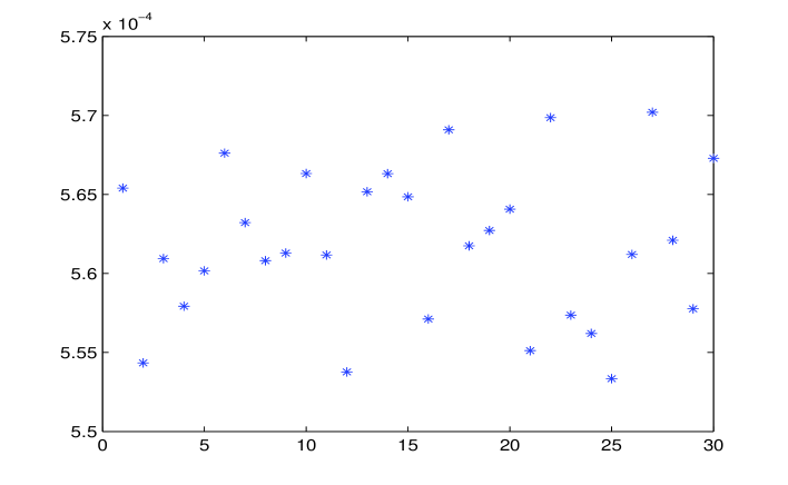
Figure 4.1. The error distribution when $N=10$.

4.2. Two dimensions

Let $\phi(x_{1},x_{2})=B_{\Xi}(x_{1},x_{2})=B_{2}(x_{1})B_{2}(x_{2})$, where $B_{2}$ is the cardinal B-spline of order $2$ defined in (3.18). By [14], $\phi(x_{1},x_{2})$ is $2$-refinable and $\phi\in H^{s}(\mathbb{R}^{2})$ with $1<s<3/2.$ Suppose that

$$f(x_{1},x_{2})=e^{-(|x_{1}|+|x_{2}|)}+e^{-(x_{1}^{2}+x_{2}^{2})}.$$

It follows from Subsection 4.1 that $e^{-(|x_{1}|+|x_{2}|)}\in H^{s}(\mathbb{R}^{2})$ where $s\in(1,3/2)$. On the other hand, $e^{-(x_{1}^{2}+x_{2}^{2})}\in H^{s}(\mathbb{R}^{2})$ for any $s\in\mathbb{R}^{+}$. Therefore $f\in H^{s}(\mathbb{R}^{2}),s\in(1,3/2)$. We next use (3.3) to approximate $f$ on $[-20,20]^{2}$. That is,

(4.3) $$f|_{[-20,20]^{2}}\approx\sum_{k\in\mathbb{Z}^{2}}f(2^{-N}(k+\varepsilon_{N,k}))\phi(2^{N}\cdot-k)\mid_{[-20,20]^{2}}.$$

The corresponding relative error is defined as

(4.4) $$\hbox{error}=||f|_{[-20,20]^{2}}-\sum_{k\in\mathbb{Z}^{2}}f(2^{-N}(k+\varepsilon_{N,k}))\phi(2^{N}\cdot-k)\mid_{[-20,20]^{2}}||_{2}/||f|_{[-20,20]^{2}}||_{2}.$$

Since $\phi$ is compactly supported, the series in (4.3) is actually involved with finite sums. On the other hand, $\lambda_{N}$ and $\theta_{N,k},k\in\mathbb{Z}^{2}$ are independent, and obey the uniform distribution on $[-1,1]^{2}$. When $N=10$, the approximation formula in (4.3) is carried out for $30$ times. See Figure 4.2 for the error distribution.

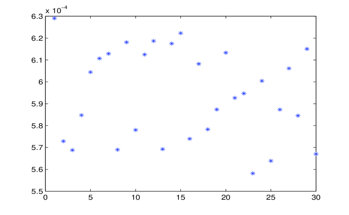
Figure 4.2. The error distribution when $N=10$.

References

- [1] A. Aldroubi, K. Gröchenig, Nonuniform sampling and reconstruction in shift-invariant spaces, SIAM Rev., 43(4), 585-620, 2001.
- [2] A. Aldroubi, I. Krishtal, Robustness of sampling and reconstruction and Beurling-Landau-type theorems for shift-invariant spaces, Appl. Comput. Harmon. Anal., 20(2), 250-260, 2006.
- [3] C. de Boor, K. Höllig, and S. Riemenschneider, Box Splines, Springer-Verlag, 1993.
- [4] J. L. Brown, Jr., On the error in reconstructing a non-bandlimited function by means of the bandpass sampling theorem, J. Math. Anal. Appl., 18, 75-84, 1967
- [5] P.L. Butzer, G. Schmeisser, R.L. Stens, The classical and approximate sampling theorems and their equivalence for entire functions of exponential type, J. Approx. Theory, 36, 143-157, 2014.
- [6] J. Chen, G. Lu, Hörmander type theorems for multi-linear and multi-parameter Fourier multiplier operators with limited smoothness, Nonlinear Analysis, 101, 98-112, 2014.
- [7] C. K. Chui, An Introduction to Wavelets, Academic Press, 1992.
- [8] C. Cheng, Y. Jiang, Q. Sun, Sampling and Galerkin reconstruction in reproducing kernel spaces, Appl. Comput. Harmon. Anal., 41(2), 638-659, 2016.
- [9] Q. Chen, T. Qian and Y. Li, Shannon-type sampling for multivariate non-bandlimited signals, Science China Mathematics, 56, 1915-1943, 2013.
- [10] P. Dang, T. Qian, Z. You, Hardy-Sobolev spaces decomposition in signal analysis, J. Fourier Anal. Appl., 17, 36-64, 2011.
- [11] I. Daubechies, Ten Lectures on Wavelets. CBMS-NSF Series in Applied Mathematics, SIAM, Philadelphia, 1992.
- [12] L. Grafakos, A. Miyachi and N. Tomita, On multilinear Fourier multipliers of limited smoothness, Canad. J. Math, 65, 299-330, 2013.
- [13] D. Han, M. Zuhair Nashed and Q. Sun, Sampling expansions in reproducing kernel Hilbert and Banach spaces, Numerical Functional Analysis and Optimization, 30(9-10), 971-987, 2009.
- [14] B. Han, Z. Shen, Dual wavelet frames and Riesz bases in Sobolev spaces, Constr. Approx., 29, 369-406, 2009.
- [15] B. Han, Computing the smoothness exponent of a symmetric multivariate refinable function, SIAM. J. Matrix Anal. & Appl., 24, 693-714, 2003.
- [16] B. Han, X. Zhuang, Analysis and construction of multivariate interpolating refinable function vectors, Acta Appl. Math., 107, 143-171, 2009.
- [17] B. Han, Pairs of frequency-based nonhomogeneous dual wavelet frames in the distribution space, Appl. Comput. Harmon. Anal., 29, 330-353, 2010.
- [18] B. Han, Nonhomogeneous wavelet systems in high dimensions, Appl. Comput. Harmon. Anal., 32, 169-196, 2012.
- [19] B. Han, Dual multiwavelet frames with high balancing order and compact fast frame transform, Appl. Comput. Harmon. Anal., 26, 14-42, 2009.
- [20] L. Hörmander, Estimates for translation invariant operators in spaces, Acta Math., 104, 93-140, 1960.
- [21] A. Krivoshein, M. Skopina, Multivariate sampling-type approximation, Analysis and Applications, 2016.
- [22] A. Krivoshein, M. Skopina, Approximation by frame-like wavelet systems, Appl. Comput. Harmon. Anal., 31(3), 410-428, 2011.
- [23] Y. Li, S. Yang, Multiwavelet sampling theorem in Sobolev spaces, Science China Mathematics, 53, 3197-3214, 2010.
- [24] Y. Li, Sampling approximation by framelets in Sobolev space and its application in modifying interpolating error, J. Approx. Theory, 175, 43-63, 2013.
- [25] Y. Li, S. Yang, D. Yuan, Bessel multiwavelet sequences and dual multiframelets in Sobolev spaces, Adv. Comput. Math., 38, 491-529, 2013.
- [26] Y. Liu, Z. Yin, Global existence and well-posedness of the viscous shallow water system in Sobolev spaces with low regularity, J. Math. Anal. Appl., 438, 14-28, 2016.
- [27] R. Schaback, A computational tool for comparing all linear PDE solvers Error-optimal methods are meshless, Adv. Comput. Math., 41, 333-355, 2015.
- [28] Mallat Stphane, A Wavelet Tour of Signal Processing, Elsevier Inc., 2009.
- [29] M. Skopina, Band-limited scaling and wavelet expansions, Appl. Comput. Harmon. Anal., 179, 94-111, 2014.
- [30] C. Shannon, A mathematical theory of communication, Bell Syst. Tech. J., 27, 379-423, 1948.
- [31] C. Shannon, Communication in the presence of noise, Proc. IRE, 37, 10-21, 1949.
- [32] Z. Song, W. Sun, X. Zhou, Z. Hou, An average sampling theorem for bandlimited stochastic processes, IEEE T. Inform. Theory, 53(12), 4798-4800, 2007.
- [33] Z. Song, B. Liu, Y. Pang, C. Hou, An improved Nyquist-Shannon irregular sampling theorem from local averages, IEEE T. Inform. Theory, 58(9), 6093 - 6100, 2012.
- [34] Q. Sun, Local reconstruction for sampling in shift-invariant spaces, Adv. Comput. Math., 32, 335-352, 2010.
- [35] Q. Sun, Nonuniform average sampling and reconstruction of signals with finite rate of innovation, SIAM Journal on Mathematical Analysis, 38, 1389-1422, 2006.
- [36] Q. Sun, Frames in spaces with finite rate of innovation, Adv. Comput. Math., 28, 301-329, 2008.
- [37] W. Sun, X. Zhou, Reconstruction of band-limited functions from local averages, Constr. Approx., 18, 205-222, 2002.
- [38] W. Sun, X. Zhou, Characterization of local sampling sequences for spline subspaces, Adv. Comput. Math., 30, 153-175, 2009.
- [39] W. Sun, Local sampling theorems for spaces generated by splines with arbitrary knots, Math. Comp., 78, 225-239, 2009.
- [40] W. Wang and C. Xu, The Cauchy problem for viscous shallow water equations, Rev. Mat. Iberoamericana, 21, 1-24, 2005.