Solving Lauricella String Scattering Amplitudes through Recurrence Relations

Abstract

We show that there exist infinite number of recurrence relations valid for all energies among the open bosonic string scattering amplitudes (SSA) of three tachyons and one arbitrary string state, or the Lauricella SSA. Moreover, these infinite number of recurrence relations can be used to solve all the Lauricella SSA and express them in terms of one single four tachyon amplitude. These results extend the solvability of SSA at the high energy, fixed angle scattering limit and those at the Regge scattering limit discovered previously to all kinematic regimes.

1
Introduction

It was widely believed that string theory consists of huge spacetime symmetries. In particular, it was conjectured GM ; Gross ; GrossManes that in the high energy fixed angle regime there existed infinite number of linear relations among string scattering ampitudes (SSA) of different string states. Moreover, these relations are so powerful that they can be used to solve all high energy SSA and express them in terms of one single four tachyon amplitude.

Since it is a nontrivial task to compute exactly infinite number of massive higher spin SSA and the corresponding exact symmetries Moore ; Moore1 ; CKT for states at general mass levels, only SSA at high energy limit and relations among them were worked out in details in the literature ChanLee1 ; ChanLee2 ; CHL ; PRL ; CHLTY ; susy LY ; LY2014 . In fact, in the high energy fixed angle regime, the existence of these infinite linear relations among SSA was conjectured by Gross GM ; Gross ; GrossManes and later corrected and explicitly proved in ChanLee1 ; ChanLee2 ; CHL ; PRL ; CHLTY ; susy by using decoupling of zero-norm states (ZNS) ZNS1 , and can be used to reduce the number of independent hard SSA from $\infty$ down to $1$.

On the other hand, it was discovered that in the high energy fixed momentum transfer regime, the Regge SSA of three tachyons and one arbitrary string states can be expressed in terms of the first Appell function $F_{1}$ LY2014 . Regge stringy symmetries or recurrence relations, instead of linear relations in the fixed angle regime, among Regge SSA LY ; LY2014 were constructed and can be used to reduce the number of independent Regge SSA from $\infty$ down to $1$. Moreover, an interesting link between Regge SSA and hard SSA was identified KLY ; LYY , and for each mass level the ratios among hard SSA can be extracted from the corresponding Regge SSA. See the recent review review for more details.

Recently a class of stringy SSA valid for all energies were exactly calculated LLY2 . These are the open bosonic SSA of three tachyons and one arbitrary string state or the so-called Lauricella string scattering amplitudes (LSSA). These LSSA were soon calculated by using the deformed cubic string field theory TL ; TL2 ; TL3 ; TL4 , and exactly the same results were reproduced LLYL consistently. This string field theory calculation LLYL can be considered as the extention of SSA calculation of low mass string states Gidd ; Samuel through second quantized string to those of infinite number of higher mass string states. One important follow-up question then is whether there exist relations among these LSSA so that one can use them to solve all the LSSA and express them in terms of one single four tachyon amplitude.

In this paper, we will show that all the LSSA calculated in LLY2 can be solved through various recurrence relations of Lauricella functions. Moreover, all the LSSA can be expressed in terms of one single amplitude, say four tachyon string scattering amplitude. These results strongly suggest the existence of a huge spacetime symmetry of open bosonic string theory associated with $SL(K+3,C)$ sl5c ; sl4c as suggested in LLY2 , and are extentions of results calculated previously for both high energy, fixed angle SSA and Regge SSA review .

In the last section of this paper, we will study the Lauricella zero norm states (LZNS) and the corresponding stringy Ward identities. In particular, we will show that the solvability of LSSA through recurrence relations imply the validity of Ward identities. However, the LZNS or the corresponding Lauricella Ward identities are not good enough to solve all the LSSA and express them in terms of one amplitude. This is in constrast to the fact that the high energy zero norm states (HZNS) at the fixed angle regime can be used to solve all the high energy SSA ChanLee1 ; ChanLee2 ; CHL ; PRL ; CHLTY ; susy and express them in terms of one single four tachyon amplitude.

2 The Lauricella String Scattering Amplitude

We first briefly review the calculation of the LSSA LLY2 of three tachyons and one arbitrary string states sitting at the second vertex. In the center of momentum frame, the kinematics are defined as

$$k_{1} =\left(\sqrt{M_{1}^{2}+|\vec{k_{1}}|^{2}},-|\vec{k_{1}}|,0\right),$$ (2.1a)

$$k_{2} =\left(\sqrt{M_{2}+|\vec{k_{1}}|^{2}},+|\vec{k_{1}}|,0\right),$$ (2.1b)

$$k_{3} =\left(-\sqrt{M_{3}^{2}+|\vec{k_{3}}|^{2}},-|\vec{k_{3}}|\cos\phi,-|\vec{k_{3}}|\sin\phi\right),$$ (2.1c)

$$k_{4} =\left(-\sqrt{M_{4}^{2}+|\vec{k_{3}}|^{2}},+|\vec{k_{3}}|\cos\phi,+|\vec{k_{3}}|\sin\phi\right)$$ (2.1d)

where $$M_{1}^{2}=M_{3}^{2}=M_{4}^{2}=-2 \phi s=-\left(k_{1}+k_{2}\right)^{2},~{}t=-\left(k_{2}+k_{3}\right)^{2},~{}u=-\left(k_{1}+k_{3}\right)^{2}$$ and is the scattering angle. The Mandelstam variables are . The three polarization vectors on the scattering plane are ChanLee1 ; ChanLee2

$$e^{T} =(0,0,1),$$ (2.2a)

$$e^{L} =\frac{1}{M_{2}}\left(|\vec{k_{1}}|,\sqrt{M_{2}+|\vec{k_{1}}|^{2}},0\right),$$ (2.2b)

$$e^{P} =\frac{1}{M_{2}}\left(\sqrt{M_{2}+|\vec{k_{1}}|^{2}},|\vec{k_{1}}|,0\right).$$ (2.2c)

Note that SSA of three tachyons and one arbitrary string state with polarizations orthogonal to the scattering plane vanish. For later use, we define

$$k_{i}^{X}\equiv e^{X}\cdot k_{i}\text{ \ for \ }X=\left(T,P,L\right).$$ (2.3)

For the $26D$ open bosonic string, the general string states at mass level $M_{2}^{2}=2(N-1)$, $N=\sum_{n,m,l>0}\left(np_{n}+mq_{m}+lr_{l}\right)$ with polarizations on the scattering plane are of the form

$$\left|p_{n},q_{m},r_{l}\right\rangle=\prod_{n>0}\left(\alpha_{-n}^{T}\right)^{p_{n}}\prod_{m>0}\left(\alpha_{-m}^{P}\right)^{q_{m}}\prod_{l>0}\left(\alpha_{-l}^{L}\right)^{r_{l}}|0,k\rangle.$$ (2.4)

The $(s,t)$ channel of the LSSA were calculated to be LLY2

$$A_{st}^{(p_{n};q_{m};r_{l})} =B\left(-\frac{t}{2}-1,-\frac{s}{2}-1\right)\prod_{n=1}\left[-(n-1)!k_{3}^{T}\right]^{p_{n}}$$

$$\prod_{m=1}\left[-(m-1)!k_{3}^{P}\right]^{q_{m}}\prod_{l=1}\left[-(l-1)!k_{3}^{L}\right]^{r_{l}}$$

$$\cdot F_{D}^{(K)}\left(\begin{array}[]{c}-\frac{t}{2}-1;\left\{-p_{1}\right\}^{1},\cdots,\left\{-p_{n}\right\}^{n},\left\{-q_{1}\right\}^{1},\cdots,\left\{-q_{m}\right\}^{m}\\ ,\left\{-r_{1}\right\}^{1},\cdots,\left\{-r_{l}\right\}^{l};\frac{u}{2}+2-N;\\ \left[1\right],\cdots,\left[1\right],\left[\tilde{z}_{1}^{P}\right],\cdots,\left[\tilde{z}_{m}^{P}\right],\left[\tilde{z}_{1}^{L}\right]...,\left[\tilde{z}_{l}^{L}\right]\end{array}\right)$$ (2.8)

$$=B\left(-\frac{t}{2}-1,-\frac{s}{2}-1\right)\prod_{n=1}\left[-(n-1)!k_{3}^{T}\right]^{p_{n}}\prod_{m=1}\left[-(m-1)!k_{3}^{P}\right]^{q_{m}}\prod_{l=1}\left[-(l-1)!k_{3}^{L}\right]^{r_{l}}$$

$$\cdot F_{D}^{(K)}\left(-\frac{t}{2}-1;R_{n}^{T},R_{m}^{P},R_{l}^{L};\frac{u}{2}+2-N;\tilde{Z}_{n}^{T},\tilde{Z}_{m}^{P},\tilde{Z}_{l}^{L}\right)$$ (2.9)

where we have defined $R_{k}^{X}\equiv\left\{-r_{1}^{X}\right\}^{1},\cdots,\left\{-r_{k}^{X}\right\}^{k}$ with $\left\{a\right\}^{n}=\underset{n}{\underbrace{a,a,\cdots,a}}$, $Z_{k}^{X}\equiv\left[z_{1}^{X}\right],\cdots,\left[z_{k}^{X}\right]$ with $\left[z_{k}^{X}\right]=z_{k0}^{X},\cdots,z_{k\left(k-1\right)}^{X}$ and $z_{k}^{X}=\left|\left(-\frac{k_{1}^{X}}{k_{3}^{X}}\right)^{\frac{1}{k}}\right|$, $z_{kk^{\prime}}^{X}=z_{k}^{X}e^{\frac{2\pi ik^{\prime}}{k}}$, $\tilde{z}_{kk^{\prime}}^{X}\equiv 1-z_{kk^{\prime}}^{X}$ for $k^{\prime}=0,\cdots,k-1$. In Eq.(2.9) the D-type Lauricella function $F_{D}^{(K)}$ is one of the four extensions of the Gauss hypergeometric function to $K$ variables and is defined as

$$F_{D}^{(K)}\left(a;b_{1},...,b_{K};c;x_{1},...,x_{K}\right)=\sum_{n_{1},\cdots,n_{K}}\frac{\left(a\right)_{n_{1}+\cdots+n_{K}}}{\left(c\right)_{n_{1}+\cdots+n_{K}}}\frac{\left(b_{1}\right)_{n_{1}}\cdots\left(b_{K}\right)_{n_{K}}}{n_{1}!\cdots n_{K}!}x_{1}^{n_{1}}\cdots x_{K}^{n_{K}}$$ (2.10)

where $(a)_{n}=a\cdot\left(a+1\right)\cdots\left(a+n-1\right)$ is the Pochhammer symbol. There was a integral representation of the Lauricella function $F_{D}^{(K)}$ discovered by Appell and Kampe de Feriet (1926) Appell

$$F_{D}^{(K)}\left(a;b_{1},...,b_{K};c;x_{1},...,x_{K}\right)$$

$$=\frac{\Gamma(c)}{\Gamma(a)\Gamma(c-a)}\int_{0}^{1}dt\,t^{a-1}(1-t)^{c-a-1}\cdot(1-x_{1}t)^{-b_{1}}(1-x_{2}t)^{-b_{2}}...(1-x_{K}t)^{-b_{K}}.$$ (2.11)

The integer $K$ in Eq.(2.9) is defined to be

$$\text{ }K=\underset{\{\text{for all }p_{j}\neq 0\}}{\sum_{j=1}^{n}j}+\underset{\{\text{for all }q_{j}\neq 0\}}{\sum_{j=1}^{m}j}+\underset{\{\text{for all }r_{j}\neq 0\}}{\sum_{j=1}^{l}j}.$$ (2.12)

For a given $K$, there can be LSSA with different mass level $N$.

3 Solving all Lauricella string scattering amplitudes

To solve all the LSSA, one key simplification of the calculation was the observation that all arguments $b_{m}$ of the Lauricella functions in the LSSA are nonpositive integers. We stress that only Lauricella functions with special arguments are used in the LSSA in Eq.(2.9). As we will see that this will be the main reason of the solvability of the LSSA.

There seem to be no recurrence relations for the Lauricella functions available in the literature. We will first generalize the $2+2$ recurrence relations of the Appell functions to the $K+2$ recurrence relations of the Lauricella functions. One can then use these $K+2$ recurrence relations to reduce all the Lauricella functions $F_{D}^{(K)}$ in the LSSA to the Gauss hypergeometry functions ${}_{2}F_{1}(a,b,c)$. The next step is to derive a multiplication theorem for the Gauss hypergeometry functions.

The two results can then be used to prove the solvability of all LSSA. In the two steps of the proof of the solvability of all the LSSA, the property of nonpositive integers in the arguments $b_{m}$ of the Lauricella functions in the LSSA plays a key role in the argument.

3.1 Recurrence Relations of the LSSA

We begin with the Appell function case with $K=2$. In the Appell case, there are four fundamental recurrence relations which link the contiguous functions

$$\left(a-b_{1}-b_{2}\right)F_{1}\left(a;b_{1},b_{2};c,x,y\right)-aF_{1}\left(a+1;b_{1},b_{2};c,x,y\right)$$

$$+b_{1}F_{1}\left(a;b_{1}+1,b_{2};c,x,y\right)+b_{2}F_{1}\left(a;b_{1},b_{2}+1;c,x,y\right) =0,$$ (3.13)

$$cF_{1}\left(a;b_{1},b_{2};c,x,y\right)-\left(c-a\right)F_{1}\left(a;b_{1},b_{2};c+1,x,y\right)$$

$$-aF_{1}\left(a+1;b_{1},b_{2};c+1,x,y\right) =0,$$ (3.14)

$$cF_{1}\left(a;b_{1},b_{2};c,x,y\right)+c\left(x-1\right)F_{1}\left(a;b_{1}+1,b_{2};c,x,y\right)$$

$$-\left(c-a\right)xF_{1}\left(a;b_{1}+1,b_{2};c+1,x,y\right) =0,$$ (3.15)

$$cF_{1}\left(a;b_{1},b_{2};c,x,y\right)+c\left(y-1\right)F_{1}\left(a;b_{1},b_{2}+1;c,x,y\right)$$

$$-\left(c-a\right)yF_{1}\left(a;b_{1},b_{2}+1;c+1,x,y\right) =0.$$ (3.16)

It is straightforward to generalize the above relations and prove the following $K+2$ recurrence relations for the $D-type$ Lauricella functions

$$\left(a-\underset{i}{\sum}b_{i}\right)F_{D}^{(K)}\left(a;b_{1},...,b_{K};c;x_{1},...,x_{K}\right)$$

$$-aF_{D}^{(K)}\left(a+1;b_{1},...,b_{K};c;x_{1},...,x_{K}\right)$$

$$+b_{1}F_{D}^{(K)}\left(a;b_{1}+1,...,b_{K};c;x_{1},...,x_{K}\right)$$

$$+...$$

$$+b_{K}F_{D}^{(K)}\left(a;b_{1},...,b_{K}+1;c;x_{1},...,x_{K}\right) =0,$$ (3.17)

$$cF_{D}^{(K)}\left(a;b_{1},...,b_{K};c;x_{1},...,x_{K}\right)$$

$$-\left(c-a\right)F_{D}^{(K)}\left(a;b_{1},...,b_{K};c+1;x_{1},...,x_{K}\right)$$

$$-aF_{D}^{(K)}\left(a+1;b_{1},...,b_{K};c+1;x_{1},...,x_{K}\right) =0,$$ (3.18)

$$cF_{D}^{(K)}\left(a;b_{1},...,b_{m},...,b_{K};c;x_{1},...,x_{m},...,x_{K}\right)$$

$$+c(x_{m}-1)F_{D}^{(K)}\left(a;b_{1},...,b_{m}+1,...,b_{K};c;x_{1},...,x_{m},...,x_{K}\right)$$

$$+(a-c)x_{m}F_{D}^{(K)}\left(a;b_{1},...,b_{m}+1,...,b_{K};c+1;x_{1},...,x_{m},...,x_{K}\right) =0$$ (3.19)

where $m=1,2,...,K.$ One notes that for $K=2$, Eq.(3.19) reduces to the Appell recurrence relations in Eq.(3.15) and Eq.(3.16).

To proceed for a fixed $K$, we first introduce two recurrence relations from Eq.(3.19) for $m=$ $i$ , $j$ ($i\neq j$)

$$cF_{D}^{(K)}+c(x_{i}-1)F_{D}^{(K)}\left(b_{i}+1\right)+(a-c)x_{i}F_{D}^{(K)}\left(b_{i}+1;c+1\right)=0,$$ (3.20)

$$cF_{D}^{(K)}+c(x_{j}-1)F_{D}^{(K)}\left(b_{j}+1\right)+(a-c)x_{j}F_{D}^{(K)}\left(b_{j}+1;c+1\right)=0$$ (3.21)

where in each of the above two equations we have omitted those arguments of $F_{D}^{(K)}$ which remain the same for all three Lauricella functions. Then we shift $b_{i}$ to $b_{i}-1$ and $b_{j}$ to $b_{j}-1$ to obtain

$$cF_{D}^{(K)}\left(b_{i}-1\right)+c(x_{i}-1)F_{D}^{(K)}+(a-c)x_{i}F_{D}^{(K)}\left(c+1\right)=0,$$ (3.22)

$$cF_{D}^{(K)}\left(b_{j}-1\right)+c(x_{j}-1)F_{D}^{(K)}+(a-c)x_{j}F_{D}^{(K)}\left(c+1\right)=0.$$ (3.23)

By multiplying $x_{j}$ and $x_{i\text{ }}$in Eq.(3.22) and Eq.(3.23) respectively, we can subtract the resulting two equations to take away the $F_{D}^{(K)}\left(c+1\right)$ term and obtain the following key recurrence relation

$$x_{j}F_{D}^{(K)}\left(b_{i}-1\right)-x_{i}F_{D}^{(K)}\left(b_{j}-1\right)+\left(x_{i}-x_{j}\right)F_{D}^{(K)}=0.$$ (3.24)

One can repeatly apply Eq.(3.24) to the Lauricella functions in the LSSA in Eq.(2.9) and end up with an expression which expresses $F_{D}^{(K)}(b_{1},b_{2},..b_{K})$ in terms of $F_{D}^{(K-1)}(b_{1},..b_{i-1},b_{i+1}..b_{j}^{\prime},..b_{K})$, $b_{j}^{\prime}=b_{j},b_{j}-1,..,b_{j}-\left|b_{i}\right|$ or $F_{D}^{(K-1)}(b_{1},..b_{i}^{\prime},..b_{j-1},b_{j+1},..b_{K})$, $b_{i}^{\prime}=b_{i},b_{i}-1,..,b_{i}-\left|b_{j}\right|$ (assume $i<j$). We can repeat the process to decrease the value of $K$ and reduce all the Lauricella functions $F_{D}^{(K)}$ in the LSSA to the Gauss hypergeometry functions $F_{D}^{(1)}=$ ${}_{2}F_{1}(a,b,c,x)$. See Figure 1 in the text.

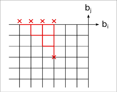
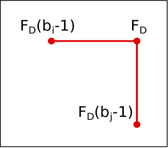
(a)                                                            (b)

Figure 1: The neighborhood points in the figures are related by the recurrence relations.

3.2 Reduction by a Multiplication Theorem

In this subsection, to further reduce the Gauss hypergeometry functions in the LSSA and solve all the LSSA in terms of one single amplitude, we first derive a multiplication theorem for the Gauss hypergeometry functions.

If we replace $y$ by $(y-1)x$ in the following Taylor’s theorem

$$f(x+y)=\sum_{n=0}^{\infty}f^{(n)}(x)\frac{y^{n}}{n!},$$ (3.25)

we get the identity

$$f(xy)=\sum_{n=0}^{\infty}\frac{(y-1)^{n}x^{n}}{n!}\frac{d^{n}}{dx^{n}}f(x).$$ (3.26)

One can now use the derivative relation of the Gauss hypergeometry function

$$\frac{d^{n}}{dx^{n}}\text{ }_{2}F_{1}(a,b,c,x)=\frac{(a)_{n}(b)_{n}}{(c)_{n}}\text{ }_{2}F_{1}(a+n,b+n,c+n,x)$$ (3.27)

where $(a)_{n}=a\cdot\left(a+1\right)\cdots\left(a+n-1\right)$ is the Pochhammer symbol to derive the following multiplication theorem

$$\text{ }_{2}F_{1}(a,b,c,xy)=\sum_{n=0}^{\left|b\right|}\frac{(y-1)^{n}x^{n}}{n!}\frac{(a)_{n}(b)_{n}}{(c)_{n}}\text{ }_{2}F_{1}(a+n,b+n,c+n,x).$$ (3.28)

It is important to note that the $\infty$ upper bound of the summation in the above equation has been replaced by $\left|b\right|$ since $b$ is a nonpositive integer for the cases of LSSA. In particular if we take $x=1$ in Eq.(3.28), we get the following relation

$$\text{ }_{2}F_{1}(a,b,c,y)=\sum_{n=0}^{\left|b\right|}\frac{(y-1)^{n}}{n!}\frac{(a)_{n}(b)_{n}}{(c)_{n}}\text{ }_{2}F_{1}(a+n,b+n,c+n,1).$$ (3.29)

The factor ${}_{2}F_{1}$ on the right hand side of the above equation can be written as

$${}_{2}F_{1}(a+n,b+n,c+n,1) =\frac{\Gamma(c+n)\Gamma(c-a-b-n)}{\Gamma(c-a)\Gamma(c-b)}$$

$$=\frac{(-)^{n}(c)_{n}}{(c-a-b)_{n}}\frac{\Gamma(c)\Gamma(c-a-b)}{\Gamma(c-a)\Gamma(c-b)}$$

$$=\frac{(-)^{n}(c)_{n}}{(c-a-b)_{n}}\text{ }_{2}F_{1}(a,b,c,1).$$ (3.30)

Finally one identifies that

$${}_{2}F_{1}(a,b,c,1)=\text{ }_{2}F_{1}(-\frac{t}{2}-1,-p_{1},\frac{u}{2}+2-p_{1},1)$$ (3.31)

which corresponds to the LSSA with the polarization $(\alpha_{-1}^{T})^{p_{1}}=(\alpha_{-1}^{T})^{-b}$ in Eq.(2.4). One can even use one of the $15$ Gauss contiguous relations

$$\{c-2b+(b-a)x\}_{2}F_{1}+b(1-x)_{2}F_{1}(b+1)+(b-c)_{2}F_{1}(b-1)=0,$$ (3.32)

and set $x=1$ which kills the second term of Eq.(3.32) to reduce $b$ in ${}_{2}F_{1}(a,b,c,1)$ to $b=-1$ or $0$ which corresponds to vector or tachyon amplitudes in the LSSA. This completes the proof that all the LSSA calculated in Eq.(2.9) can be solved through various recurrence relations of Lauricella functions. Moreover, all the LSSA can be expressed in terms of one single four tachyon amplitude.

For illustration, in the following, we calculate the Lauricella functions which correspond to the LSSA for levels $K=1,2,3$. For $K=1$ there are three type of LSSA $(a=-\frac{t}{2}-1,c=\frac{u}{2}+2)$

$$(\alpha_{-1}^{T})^{p_{1}}\text{ , }F_{D}^{(1)}(a,-p_{1},,c-p_{1},1)\text{ , }N =p_{1},$$ (3.33)

$$(\alpha_{-1}^{P})^{q_{1}}\text{ , }F_{D}^{(1)}(a,-q_{1},c-q_{1},\left[\tilde{z}_{1}^{P}\right])\text{ , }N =q_{1},$$ (3.34)

$$(\alpha_{-1}^{L})^{r_{1}}\text{ , }F_{D}^{(1)}(a,-r_{1},c-r_{1},\left[\tilde{z}_{1}^{L}\right])\text{ , }N =r_{1}.$$ (3.35)

For $K=2$ there are six type of LSSA $(\omega=-1)$

$$(\alpha_{-1}^{T})^{p_{1}}(\alpha_{-1}^{P})^{q_{1}}\text{,}F_{D}^{(2)}(a,-p_{1},-q_{1},c-p_{1}-q_{1},1,\left[\tilde{z}_{1}^{P}\right])\text{,}N =p_{1}+q_{1},$$ (3.36)

$$(\alpha_{-1}^{T})^{p_{1}}(\alpha_{-1}^{L})^{r_{1}}\text{,}F_{D}^{(2)}(a,-p_{1},-r_{1},c-p_{1}-r_{1},1,\left[\tilde{z}_{1}^{L}\right])\text{,}N =p_{1}+r_{1},$$ (3.37)

$$(\alpha_{-1}^{P})^{q_{1}}(\alpha_{-1}^{L})^{r_{1}}\text{,}F_{D}^{(2)}(a,-q_{1},-r_{1},c-q_{1}-r_{1},\left[\tilde{z}_{1}^{P}\right],\left[\tilde{z}_{1}^{L}\right])\text{,}N =q_{1}+r_{1},$$ (3.38)

$$(\alpha_{-2}^{T})^{p_{2}}\text{ , }F_{D}^{(2)}(a,-p_{2},-p_{2},c-2p_{2},1,1)\text{ , }N =2p_{2},$$ (3.39)

$$(\alpha_{-2}^{P})^{q_{2}}\text{ , }F_{D}^{(2)}(a,-q_{2},-q_{2},c-2q_{2},1-Z_{2}^{P},1-\omega Z_{2}^{P}),N =2q_{2},$$ (3.40)

$$(\alpha_{-2}^{L})^{r_{2}}\text{ , }F_{D}^{(2)}(a,-r_{2},-r_{2},c-2r_{2},1-Z_{2}^{L},1-\omega Z_{2}^{L}),N =2r_{2}.$$ (3.41)

For $K=3$, there are ten type of LSSA $(\omega_{1}=-1,\omega_{2}=\frac{-1+i\sqrt{3}}{2})$

$$(\alpha_{-1}^{T})^{p_{1}}(\alpha_{-1}^{P})^{q_{1}}(\alpha_{-1}^{L})^{r_{1}},F_{D}^{(3)}(a,-p_{1},-q_{1},-r_{1},c-p_{1}-q_{1}-r_{1},1,\left[\tilde{z}_{1}^{P}\right],\left[\tilde{z}_{1}^{L}\right]),N =p_{1}+q_{1}+r_{1},$$ (3.42)

$$(\alpha_{-2}^{T})^{p_{2}}(\alpha_{-1}^{P})^{q_{1}}\text{,}F_{D}^{(3)}(a,-p_{2},-p_{2},-q_{1},c-2p_{2}-q_{1},1,1,\left[\tilde{z}_{1}^{P}\right]),N =2p_{2}+q_{1},$$ (3.43)

$$(\alpha_{-2}^{T})^{p_{2}}(\alpha_{-1}^{L})^{r_{1}}\text{,}F_{D}^{(3)}(a,-p_{2},-p_{2},-r_{1},c-2p_{2}-r_{1},1,1,\left[\tilde{z}_{1}^{L}\right]),N =2p_{2}+r_{1},$$ (3.44)

$$(\alpha_{-1}^{T})^{p_{1}}(\alpha_{-2}^{P})^{q_{2}}\text{,}F_{D}^{(3)}(a,-p_{1},-q_{2},-q_{2},c-2q_{2}-p_{1},1,1-Z_{2}^{P},1-\omega_{1}Z_{2}^{P}),N =2q_{2}+p_{1},$$ (3.45)

$$(\alpha_{-2}^{P})^{q_{2}}(\alpha_{-1}^{L})^{r_{1}},F_{D}^{(3)}(a,-q_{2},-q_{2},-r_{1},c-2q_{2}-r_{1},1-Z_{2}^{P},1-\omega_{1}Z_{2}^{P},\left[\tilde{z}_{1}^{L}\right]),N =2q_{2}+r_{1},$$ (3.46)

$$(\alpha_{-1}^{T})^{p_{1}}(\alpha_{-2}^{L})^{r_{2}}\text{ , }F_{D}^{(3)}(a,,-p_{1},-r_{2},-r_{2},c-2r_{2}-p_{1},1,1-Z_{2}^{L},1-\omega_{1}Z_{2}^{L}),N =2r_{2}+p_{1}.$$ (3.47)

$$(\alpha_{-1}^{P})^{q_{1}}(\alpha_{-2}^{L})^{r_{2}}\text{ , }F_{D}^{(3)}(a,,-q_{1},-r_{2},-r_{2},c-2r_{2}-q_{1},\left[\tilde{z}_{1}^{P}\right],1-Z_{2}^{L},1-\omega_{1}Z_{2}^{L}),N =2r_{2}+q_{1}.$$ (3.48)

$$(\alpha_{-3}^{T})^{p_{3}}\text{ , }F_{D}^{(3)}(a,-p_{3},-p_{3},-p_{3},c-3p_{3},1,1,1),N =3p_{3},$$ (3.49)

$$(\alpha_{-3}^{P})^{q_{3}}\text{ , }F_{D}^{(3)}(a,-q_{3},-q_{3},-q_{3},c-3q_{3},1-Z_{3}^{P},1-\omega_{2}Z_{3}^{P},1-\omega_{2}^{2}Z_{3}^{P}),N =3q_{3},$$ (3.50)

$$(\alpha_{-3}^{L})^{r_{3}}\text{ , }F_{D}^{(3)}(a,-r_{3},-r_{3},-r_{3},c-3r_{3},1-Z_{3}^{L},1-\omega_{2}Z_{3}^{L},1-\omega_{2}^{2}Z_{3}^{L}),N =3r_{3}.$$ (3.51)

All the LSSA for $K=2,3$ can be reduced through the recurrence relations in Eq.(3.24) and expressed in terms of those of $K=1.$ Furthermore, all resulting LSSA for $K=1$ can be further reduced by applying Eq.(3.29) to Eq.(3.32) and finally expressed in terms of one single LSSA.

4 Lauricella Zero Norm States and Ward Identities

In addition to the recurrence relations among LSSA, there are on-shell stringy Ward identities among LSSA. These Ward identities can be derived from the decoupling of two type of zero norm states (ZNS) in the old covariant first quantized string spectrum. However, as we will see soon that these Lauricella zero norm states (LZNS) or the corresponding Lauricella Ward identities are not good enough to solve all the LSSA and express them in terms of one amplitude.

On the other hand, in the last section, we have shown that by using (A) Recurrence relations of the LSSA, (B) Multiplication theorem of Gauss hypergeometry function and (C) the explicit calculation of four tachyon amplitude, one can explicitly solve and calculate all LSSA. This means that the solvability of LSSA through the calculations of (A), (B) and (C) imply the validity of Ward identities. Ward identities can not be identities independent of recurrence relations we used in the last section. Otherwise there will be a contradiction with the solvabilibity of LSSA.

In this section, we will study some examples of Ward identities of LSSA from this point of view. Incidentally, high energy zero norm states (HZNS) ChanLee1 ; ChanLee2 ; CHL ; PRL ; CHLTY ; susy and the corresponding stringy Ward identities at the fixed angle regime, and Regge zero norm states (RZNS) LY ; LY2014 and the corresponding Regge Ward identities at the Regge regime have been studied previously. In particular, HZNS at the fixed angle regime can be used to solve all the high energy SSA ChanLee1 ; ChanLee2 ; CHL ; PRL ; CHLTY ; susy .

4.1 The Lauricella zero norm states

We will consider a smaller set of Ward identities, namely, those among the LSSA or string scattering amplitudes with three tachyons and one arbitrary string states. So we need only consider polarizations of the tensor states on the scattering plane. There are two types of zero norm states (ZNS) in the old covariant first quantum string spectrum

$$\text{Type I}:L_{-1}\left|x\right\rangle,\text{ where }L_{1}\left|x\right\rangle=L_{2}\left|x\right\rangle=0,\text{ }L_{0}\left|x\right\rangle=0;$$ (4.52)

$$\text{Type II}:(L_{-2}+\frac{3}{2}L_{-1}^{2})\left|\widetilde{x}\right\rangle,\text{ where }L_{1}\left|\widetilde{x}\right\rangle=L_{2}\left|\widetilde{x}\right\rangle=0,\text{ }(L_{0}+1)\left|\widetilde{x}\right\rangle=0.$$ (4.53)

While type I states have zero-norm at any spacetime dimension, type II states have zero-norm only at $D=26$.

We begin with the case of mass level $M^{2}=2$. There is a type II ZNS

$$\left[\frac{1}{2}\alpha_{-1}\cdot\alpha_{-1}+\frac{5}{2}k\cdot\alpha_{-2}+\frac{3}{2}(k\cdot\alpha_{-1})^{2}\right]\left|0,k\right\rangle$$ (4.54)

and a type I ZNS

$$[\theta\cdot\alpha_{-2}+(k\cdot\alpha_{-1})(\theta\cdot\alpha_{-1})]\left|0,k\right\rangle,\theta\cdot k=0.$$ (4.55)

Note that for the LSSA of three tachyons and one arbitrary string state, amplitudes with polarizations orthogonal to the scattering plane vanish. We define the polarizations of the 2nd tensor state with momentum $k_{2}$ on the scattering plane to be $e_{P}=\frac{1}{M_{2}}(E_{2},\mathrm{k}_{2},0)=\frac{k_{2}}{M_{2}}$ $($or $e^{P}=\frac{1}{M_{2}}(-E_{2},\mathrm{k}_{2},0))$ as the momentum polarization, $e^{L}=\frac{1}{M_{2}}(\mathrm{k}_{2},E_{2},0)$ the longitudinal polarization and $e^{T}=(0,0,1)$ the transverse polarization. $\eta_{\mu\nu}=diag(-1,1,1).$ The three vectors $e^{P}$, $e^{L}$ and $e^{T}$ satisfy the completeness relation

$$\eta_{\mu\nu}=\sum_{\alpha,\beta}e_{\mu}^{\alpha}e_{\nu}^{\beta}\eta_{\alpha\beta}$$ (4.56)

where $\mu,\nu=0,1,2$ and $\alpha,\beta=P,L,T$ and $\alpha_{-1}^{T}=\sum_{\mu}e_{\mu}^{T}\alpha_{-1}^{\mu}$, $\alpha_{-1}^{T}\alpha_{-2}^{L}=\sum_{\mu,\nu}e_{\mu}^{T}e_{\nu}^{L}\alpha_{-1}^{\mu}\alpha_{-2}^{\nu}$ etc.

The type II ZNS in Eq.(4.54) gives the LZNS

$$(\sqrt{2}\alpha_{-2}^{P}+\alpha_{-1}^{P}\alpha_{-1}^{P}+\frac{1}{5}\alpha_{-1}^{L}\alpha_{-1}^{L}+\frac{1}{5}\alpha_{-1}^{T}\alpha_{-1}^{T})|0,k\rangle.$$ (4.57)

Type I ZNS in Eq.(4.55) gives two LZNS

$$(\alpha_{-2}^{T}+\sqrt{2}\alpha_{-1}^{P}\alpha_{-1}^{T})|0,k\rangle,$$ (4.58)

$$(\alpha_{-2}^{L}+\sqrt{2}\alpha_{-1}^{P}\alpha_{-1}^{L})|0,k\rangle.$$ (4.59)

LZNS in Eq.(4.58) and Eq.(4.59) correspond to choose $\theta^{\mu}=e^{T}$ and $\theta^{\mu}=e^{L}$ respectively. In conclusion, there are $3$ LZNS at the mass level $M^{2}=$ $2$.

At the second massive level $M^{2}=4,$ there is a type I scalar ZNS

$$[\frac{17}{4}(k\cdot\alpha_{-1})^{3}+\frac{9}{2}(k\cdot\alpha_{-1})(\alpha_{-1}\cdot\alpha_{-1})+9(\alpha_{-1}\cdot\alpha_{-2})$$

$$+21(k\cdot\alpha_{-1})(k\cdot\alpha_{-2})+25(k\cdot\alpha_{-3})]\left|0,k\right\rangle,$$ (4.60)

a symmetric type I spin two ZNS

$$[2\theta_{\mu\nu}\alpha_{-1}^{(\mu}\alpha_{-2}^{\nu)}+k_{\lambda}\theta_{\mu\nu}\alpha_{-1}^{\lambda\mu\nu}]\left|0,k\right\rangle,k\cdot\theta=\eta^{\mu\nu}\theta_{\mu\nu}=0,\theta_{\mu\nu}=\theta_{\nu\mu}$$ (4.61)

where $\alpha_{-1}^{\lambda\mu\nu}\equiv\alpha_{-1}^{\lambda}\alpha_{-1}^{\mu}\alpha_{-1}^{\nu}$ and two vector ZNS

$$\left[(\frac{5}{2}k_{\mu}k_{\nu}\theta_{\lambda}^{\prime}+\eta_{\mu\nu}\theta_{\lambda}^{\prime})\mathcal{\alpha}_{-1}^{(\mu\nu\lambda)}+9k_{\mu}\theta_{\nu}^{\prime}\mathcal{\alpha}_{-1}^{(\mu\nu)}+6\theta_{\mu}^{\prime}\mathcal{\alpha}_{-1}^{\mu}\right]\left|0,k\right\rangle,\theta\cdot k =0,$$ (4.62)

$$\left[(\frac{1}{2}k_{\mu}k_{\nu}\theta_{\lambda}+2\eta_{\mu\nu}\theta_{\lambda})\mathcal{\alpha}_{-1}^{(\mu\nu\lambda)}+9k_{\mu}\theta_{\nu}\mathcal{\alpha}_{-1}^{[\mu\nu]}-6\theta_{\mu}\mathcal{\alpha}_{-1}^{\mu}\right]\left|0,k\right\rangle,\theta\cdot k =0.$$ (4.63)

Note that Eq.(4.62) and Eq.(4.63) are linear combinations of a type I and a type II ZNS. This completes the four ZNS at the second massive level $M^{2}=$ $4$.

The scalar ZNS in Eq.(4.60) gives the LZNS

$$[25(\alpha_{-1}^{P})^{3}+9\alpha_{-1}^{P}(\alpha_{-1}^{L})^{2}+9\alpha_{-1}^{P}(\alpha_{-1}^{T})^{2}+9\alpha_{-2}^{L}\alpha_{-1}^{L}+9\alpha_{-2}^{T}\alpha_{-1}^{T}+75\alpha_{-2}^{P}\alpha_{-1}^{P}+50\alpha_{-3}^{P}]\left|0,k\right\rangle.$$ (4.64)

For the type I spin two ZNS in Eq.(4.61), we define

$$\theta_{\mu\nu}=\sum_{\alpha,\beta}e_{\mu}^{\alpha}e_{\nu}^{\beta}u_{\alpha\beta},$$ (4.65)

symmetric and transverse conditions on $\theta_{\mu\nu}$ then implies

$$u_{\alpha\beta}=u_{\beta\alpha};u_{PP}=u_{PL}=u_{PT}=0.$$ (4.66)

The traceless condition on $\theta_{\mu\nu}$ implies

$$u_{PP}-u_{LL}-u_{TT}=0.$$ (4.67)

Eq.(4.66) and Eq.(4.67) give two LZNS

$$(\alpha_{-1}^{L}\alpha_{-2}^{L}+\alpha_{-1}^{P}\alpha_{-1}^{L}\alpha_{-1}^{L}-\alpha_{-1}^{T}\alpha_{-2}^{T}-\alpha_{-1}^{P}\alpha_{-1}^{T}\alpha_{-1}^{T})|0,k\rangle,$$ (4.68)

$$(\alpha_{-1}^{(L}\alpha_{-2}^{T)}+\alpha_{-1}^{P}\alpha_{-1}^{L}\alpha_{-1}^{T})|0,k\rangle.$$ (4.69)

The vector ZNS in Eq.(4.62) gives two LZNS

$$[6\alpha_{-3}^{T}+18\alpha_{-1}^{(P}\alpha_{-2}^{T)}+9\alpha_{-1}^{P}\alpha_{-1}^{P}\alpha_{-1}^{T}+\alpha_{-1}^{L}\alpha_{-1}^{L}\alpha_{-1}^{T}+\alpha_{-1}^{T}\alpha_{-1}^{T}\alpha_{-1}^{T}]|0,k\rangle,$$ (4.70)

$$[6\alpha_{-3}^{L}+18\alpha_{-1}^{(P}\alpha_{-2}^{L)}+9\alpha_{-1}^{P}\alpha_{-1}^{P}\alpha_{-1}^{L}+\alpha_{-1}^{L}\alpha_{-1}^{L}\alpha_{-1}^{L}+\alpha_{-1}^{L}\alpha_{-1}^{T}\alpha_{-1}^{T}]|0,k\rangle.$$ (4.71)

The vector ZNS in Eq.(4.63) gives two LZNS

$$[3\alpha_{-3}^{T}-9\alpha_{-1}^{[P}\alpha_{-2}^{T]}-\alpha_{-1}^{L}\alpha_{-1}^{L}\alpha_{-1}^{T}-\alpha_{-1}^{T}\alpha_{-1}^{T}\alpha_{-1}^{T}]|0,k\rangle,$$ (4.72)

$$[3\alpha_{-3}^{L}-9\alpha_{-1}^{[P}\alpha_{-2}^{L]}-\alpha_{-1}^{L}\alpha_{-1}^{L}\alpha_{-1}^{L}-\alpha_{-1}^{L}\alpha_{-1}^{T}\alpha_{-1}^{T}]|0,k\rangle.$$ (4.73)

In conclusion, there are totally $7$ LZNS at the mass level $M^{2}=$ $4$.

It is important to note that there are $9$ LSSA at mass level $M^{2}=$ $2$ with only $3$ LZNS, and $22$ LSSA at mass level $M^{2}=$ $4$ with only $7$ LZNS. So in constrast to the recurrence relations calculated in Eq.(3.24) and Eq.(3.28), these Ward identities are not good enough to solve all the LSSA and express them in terms of one amplitude.

4.2 The Lauricella Ward identities

In this subsection, we will explicitly verify some examples of Ward identities through processes (A),(B) and (C). Process (C) will be implicitly used through the kinematics. Ward identities can not be identities independent of recurrence relations we used in processes (A),(B) and (C) in the last section. We define the following kinematics variables (for $M^{2}=$ $2$)

$$a=\frac{-t}{2}-1=Mk_{3}^{P}-N+1=\sqrt{2}k_{3}^{P}-1,$$ (4.74)

$$c=\frac{s}{2}+2-N=-Mk_{1}^{P}=-\sqrt{2}k_{1}^{P},$$ (4.75)

$$d=\left(\frac{-k_{1}^{L}}{k_{3}^{L}}\right)^{\frac{1}{2}},1-\left(\frac{-k_{1}^{P}}{k_{3}^{P}}\right)=\frac{a-c+1}{a+1},$$ (4.76)

then

$$\frac{u}{2}+2-N=a-c+1-N=a-c-1.$$ (4.77)

As the first example, we calculate the Ward identity associated with the LZNS in Eq.(4.58). The calculation will be based on processes (A) and (B). By using Eq.(2.9), the Ward identity we want to prove is

$$\left(-k_{3}^{T}\right)F_{D}^{(2)}\left(a;-1,-1;a-c-1;1-\left(\frac{-k_{1}^{T}}{k_{3}^{T}}\right)^{\frac{1}{2}},1+\left(\frac{-k_{1}^{T}}{k_{3}^{T}}\right)^{\frac{1}{2}}\right)$$

$$+\sqrt{2}\left(-k_{3}^{P}\right)\left(-k_{3}^{T}\right)F_{D}^{(2)}\left(a;-1,-1;a-c-1;1-\left(\frac{-k_{1}^{P}}{k_{3}^{P}}\right),1-\left(\frac{-k_{1}^{T}}{k_{3}^{T}}\right)\right)=0$$ (4.78)

or

$$F_{D}^{(2)}(a;-1,-1;a-c-1;1,1)-(a+1)F_{D}^{(2)}\left(a;-1,-1;a-c-1;\frac{a-c+1}{a+1},1\right)=0.$$ (4.79)

Now let’s make use of Eq.(3.24) in the process (A) to the first term of Eq.(4.79). We get

$$1\times F_{D}^{(2)}(a;-2,0;a-c-1;1,1)$$

$$-1\times F_{D}^{(2)}(a;-1,-1;a-c-1;1,1)$$

$$+(1-1)F_{D}^{(2)}(a,;-1,0;a-c-1;1,1) =0,$$ (4.80)

which means

$$F_{D}^{(2)}(a;-1,-1;a-c-1;1)=F_{D}^{(1)}(a;-2;a-c-1;1).$$ (4.81)

Similar calculation can be applied to the second term of Eq.(4.79), which can be reduced to

$$F_{D}^{(2)}\left(a;-1,-1;a-c-1;\frac{a-c+1}{a+1},1\right)$$

$$=\frac{a-c+1}{a+1}F_{D}^{(1)}\left(a;-2;a-c-1;1\right)+\frac{c}{a+1}F_{D}^{(1)}\left(a;-1;a-c-1;1\right).$$ (4.82)

Finally the Ward identity in Eq.(4.79) is explicitly verified through processe (A)

$$F_{D}^{(2)}(a;-1,-1;a-c-1;1,1)-(a+1)F_{D}^{(2)}\left(a;-1,-1;a-c-1;\frac{a-c+1}{a+1},1\right)$$

$$=F_{D}^{(1)}(a;-2;a-c-1;1)-(a+1)$$

$$\times\left[\frac{a-c+1}{a+1}F_{D}^{(1)}\left(a;-2;a-c-1;1\right)+\frac{c}{a+1}F_{D}^{(1)}\left(a;-1;a-c-1;1\right)\right]$$

$$=(c-a)F_{D}^{(1)}\left(a;-2;a-c-1;1\right)-cF_{D}^{(1)}\left(a;-1;a-c-1;1\right)$$

$$=0$$ (4.83)

where Eq.(3.32) has been used to get the last equality of the above equation.

As the second example, we calculate the Ward identity associated with the LZNS in Eq.(4.59). By using Eq.(2.9), the Ward identity is

$$\left(-k_{3}^{L}\right)F_{D}^{(2)}\left(a;-1,-1;a-c-1;1-\left(\frac{-k_{1}^{L}}{k_{3}^{L}}\right)^{\frac{1}{2}},1+\left(\frac{-k_{1}^{L}}{k_{3}^{L}}\right)^{\frac{1}{2}}\right)$$

$$+\sqrt{2}\left(-k_{3}^{P}\right)\left(-k_{3}^{L}\right)F_{D}^{(2)}\left(a;-1,-1;a-c-1;1-\left(\frac{-k_{1}^{P}}{k_{3}^{P}}\right),1-\left(\frac{-k_{1}^{L}}{k_{3}^{L}}\right)\right)=0$$ (4.84)

or

$$F_{D}^{(2)}(a;-1,-1;a-c-1;1-d,1+d)$$

$$-(a+1)F_{D}^{(2)}\left(a;-1,-1;a-c-1;\frac{a-c+1}{a+1},1-d^{2}\right)=0.$$ (4.85)

Now let’s make use of Eq.(3.24) in the process (A) to the first term of Eq.(4.85). We get

$$F_{D}^{(2)}F(a;-1,-1;a-c-1;1-d,1+d)$$

$$=\frac{1-d}{1+d}F_{D}^{(1)}(a;-2;a-c-1;1+d)-\frac{2d}{1+d}F_{D}^{(1)}(a;-1;a-c-1;1+d).$$ (4.86)

We then use Eq.(3.28) and Eq.(3.30) in the prosess (B) to simplify the first term and the second term on the r.h.s. of Eq.(4.86) to be

$$F_{D}^{(1)}(a;-2;a-c-1;1+d)=F_{D}^{(1)}(a;-2;a-c-1;1)\left[1-\frac{2ad}{c-1}+\frac{a(a+1)^{2}}{(c-1)(c-2)}\right]$$

and

$$F_{D}^{(1)}(a;-1;a-c-1;1+d)=F_{D}^{(1)}(a;-1;a-c-1;1)\left[1-\frac{ad}{c}\right].$$

We now use Eq.(3.24) in the process (A) to the second term of Eq.(4.85) to get

$$F_{D}^{(2)}\left(a;-1,-1;a-c-1;\frac{a-c+1}{a+1},1-d^{2}\right)$$

$$=\left[\frac{a-c+1}{(a+1)(1-d^{2})}\right]F_{D}^{(1)}\left(a;-2;a-c-1;1-d^{2}\right)$$

$$-\left[\frac{a-c+1}{(a+1)(1-d^{2})}-(1-d)\right]F_{D}^{(1)}F(a;-1;a-c-1;1-d^{2})$$ (4.87)

We then use Eq.(3.28) and Eq.(3.30) in the prosess (B) to simplify the first term and the second term on the r.h.s. of Eq.(4.87) to be

$$F_{D}^{(1)}(a;-2;a-c-1;1-d^{2})$$

$$=\left[1+\frac{2ad^{2}}{c-1}+\frac{a(a+1)d^{4}}{(c-1)(c-2)}\right]F_{D}^{(1)}(a;-2;a-c-1,1)$$ (4.88)

and

$$F_{D}^{(1)}(a;-1;a-c-1;1-d^{2})$$

$$=\left(1+\frac{ad^{2}}{c}\right)F_{D}^{(1)}F(a;-1;a-c-1,1).$$ (4.89)

Finally we put all results to Eq.(4.85) and end up with

$$F_{D}^{(2)}(a;-1,-1;a-c-1;1-d,1+d)$$

$$-(a+1)F_{D}^{(2)}\left(a;-1,-1;a-c-1;\frac{a-c+1}{a+1},1-d^{2}\right)$$

$$=\frac{1-d}{1+d}F_{D}^{(1)}(a;-2;a-c-1;1+d)$$

$$-\frac{2d}{1+d}F_{D}^{(1)}(a;-1;a-c-1,1+d)$$

$$-(a+1)\left[\frac{a-c+1}{(a+1)(1-d^{2})}\right]F_{D}^{(1)}\left(a;-2;a-c-1;1-d^{2}\right)$$

$$+(a+1)\left[\frac{a-c+1}{(a+1)(1-d^{2})}-(1-d)\right]F_{D}^{(1)}(a;-1;a-c-1;1-d^{2})$$

$$=\frac{1-d}{1+d}\left[1-\frac{2ad}{c-1}+\frac{a(a+1)^{2}}{(c-1)(c-2)}\right]F_{D}^{(1)}(a;-2;a-c-1;1)$$

$$-\frac{2d}{1+d}\left[1-\frac{ad}{c}\right]F_{D}^{(1)}(a;-1;a-c-1;1)$$

$$-(a+1)\left[\frac{a-c+1}{(a+1)(1-d^{2})}\right]\left[1+\frac{2ad^{2}}{c-1}+\frac{a(a+1)d^{4}}{(c-1)(c-2)}\right]F_{D}^{(1)}(a;-2;a-c-1;1)$$

$$+(a+1)\left[\frac{a-c+1}{(a+1)(1-d^{2})}-(1-d)\right]\left(1+\frac{ad^{2}}{c}\right)F_{D}^{(1)}(a;-1;a-c-1;1)$$

$$=0$$ (4.90)

where again Eq.(3.32) has been used to get the last equality of the above equation.

5 Conclusions

In this paper we have shown that there exist infinite number of recurrence relations valid for all energies among the LSSA of three tachyons and one arbitrary string state. Moreover, these infinite number of recurrence relations can be used to solve all the LSSA and express them in terms of one single four tachyon amplitude. It will be interesting to see the relationship between the solvability of LSSA and the associated $SL(K+3,C)$ sl5c ; sl4c symmetry of the Lauricella functions as suggested in LLY2 . The results of this calculation extend the solvability of SSA at the high energy, fixed angle scattering limit ChanLee1 ; ChanLee2 ; CHL ; PRL ; CHLTY ; susy and those at the Regge scattering limit LY ; LY2014 discovered previously.

We have also shown that for the first few mass levels the solvability of LSSA through the calculations of recurrence relations implies the validity of Ward identities derived from the decoupling of LZNS. However the Lauricella Ward identities are not good enough to solve all the LSSA and express them in terms of one amplitude.

The extention of results for the one tensor three tachyon scatterings calculated in this paper to multi-tensor scatterings is currently under investigation.

References

• (1) D. J. Gross and P. F. Mende, Phys. Lett. B 197, 129 (1987); Nucl. Phys. B 303, 407 (1988).
• (2) D. J. Gross, Phys. Rev. Lett. 60, 1229 (1988); D. J. Gross and J. R. Ellis, Phil. Trans. R. Soc. Lond. A329, 401 (1989).
• (3) D. J. Gross and J. L. Manes, Nucl. Phys. B 326, 73 (1989). See section 6 for details.
• (4) Gregory Moore, Finite in all directions. arXiv:hep-th/9305139, 1993.
• (5) Gregory Moore, Symmetries of the bosonic string S-matrix. arXiv:hep-th/9310026,1993.
• (6) C.T. Chan, S. Kawamoto and D. Tomino, Nucl. Phys. B 885, 225 (2014).
• (7) C. T. Chan and J. C. Lee, Phys. Lett. B 611, 193 (2005). J. C. Lee, [arXiv:hep-th/0303012].
• (8) C. T. Chan and J. C. Lee, Nucl. Phys. B 690, 3 (2004).
• (9) C. T. Chan, P. M. Ho and J. C. Lee,Nucl. Phys. B 708, 99 (2005).
• (10) C. T. Chan, P. M. Ho, J. C. Lee, S. Teraguchi and Y. Yang, Phys. Rev. Lett. 96 (2006) 171601, [arXiv:hep-th/0505035].
• (11) C. T. Chan, P. M. Ho, J. C. Lee, S. Teraguchi and Y. Yang, Nucl. Phys. B 725, 352 (2005).
• (12) C. T. Chan, J. C. Lee and Y. Yang, Nucl. Phys. B 738, 93 (2006).
• (13) J.C. Lee and Y. Mitsuka, JHEP 1304:082 (2013).
• (14) J.C. Lee and Y. Yang, Phys. Lett. B739, 370 (2014).
• (15) J. C. Lee, Phys. Lett. B 241, 336 (1990); Phys. Rev. Lett. 64, 1636 (1990). J. C. Lee and B. Ovrut, Nucl. Phys. B 336, 222 (1990).
• (16) S.L. Ko, J.C. Lee and Y. Yang, JHEP, 9060:028 (2009).
• (17) J.C. Lee, C. H. Yan, and Y. Yang, ”High energy string scattering amplitudes and signless Stirling number identity”, SIGMA, 8:045, (2012).
• (18) J.C. Lee and Y. Yang, Review on High energy String Scattering Amplitudes and Symmetries of String Theory, arXiv: 1510.03297.
• (19) S.H. Lai, J.C. Lee and Y. Yang, ”The Lauricella functions and exact string scattering amplitudes”, JHEP 1611 (2016) 062, arXiv: 1609.06014.
• (20) T. Lee, Phys. Lett. B 768, 248 (2017).
• (21) T. Lee, Covariant open bosonic string field theory on multiple D-branes in the proper-time gauge, arXiv:1609.01473 [hep-th].
• (22) T. Lee, Ann. Phys. 183, 191 (1988).
• (23) T. Lee, Covariant Open String Field Theory on Multiple Dp-Branes, arXiv:1703.06402 [hep-th].
• (24) S.H. Lai, J.C. Lee, Y. Yang and T. Lee, ”String scattering amplitudes and deformed cubic string field theory”, arXiv: 1706.08025.
• (25) S. B. Giddings, Nucl. Phys. B 278, 242 (1986).
• (26) S. Samuel, Nucl. Phys. B308, 285 (1988).
• (27) Willard Miller. Jr., ”Lie theory and the Appell functions $F_{1}$”, SIAM J. Math. Anal. Vol. 4 No. 4, 638 (1973).
• (28) Willard Miller. Jr., ”Lie theory and generalizations of the hypergeometric functions”, SIAM J. Appl. Math. Vol. 25 No. 2, 226 (1973).
• (29) Joseph Kampe de Feriet and Paul Appell. Fonctions hypergeometriques et hyperspheriques 1926.