Data-Driven Sparse Structure Selection for Deep Neural Networks

Abstract

Deep convolutional neural networks have liberated its extraordinary power on various tasks. However, it is still very challenging to deploy state-of-the-art models into real-world applications due to their high computational complexity. How can we design a compact and effective network without massive experiments and expert knowledge? In this paper, we propose a simple and effective framework to learn and prune deep models in an end-to-end manner. In our framework, a new type of parameter – scaling factor is first introduced to scale the outputs of specific structures, such as neurons, groups or residual blocks. Then we add sparsity regularizations on these factors, and solve this optimization problem by a modified stochastic Accelerated Proximal Gradient (APG) method. By forcing some of the factors to zero, we can safely remove the corresponding structures, thus prune the unimportant parts of a CNN. Comparing with other structure selection methods that may need thousands of trials or iterative fine-tuning, our method is trained fully end-to-end in one training pass without bells and whistles. We evaluate our method, Sparse Structure Selection with several state-of-the-art CNNs, and demonstrate very promising results with adaptive depth and width selection. Code is available at: https://github.com/huangzehao/sparse-structure-selection.

1 Introduction

Deep learning methods, especially convolutional neural networks (CNNs) have achieved remarkable performances in many fields, such as computer vision, natural language processing and speech recognition. However, these extraordinary performances are at the expense of high computational and storage demand. Although the power of modern GPUs has skyrocketed in the last years, these high costs are still prohibitive for CNNs to deploy in latency critical applications such as self-driving cars and augmented reality, etc.

Recently, a significant amount of works on accelerating CNNs at inference time have been proposed. Methods focus on accelerating pre-trained models include direct pruning [9, 24, 29, 13, 27], low-rank decomposition [7, 20, 49], and quantization [31, 6, 44]. Another stream of researches trained small and efficient networks directly, such as knowledge distillation [14, 33, 35], novel architecture designs [18, 15] and sparse learning [25, 50, 1, 43]. In spare learning, prior works [25] pursued the sparsity of weights. However, non-structure sparsity only produce random connectivities and can hardly utilize current off-the-shelf hardwares such as GPUs to accelerate model inference in wall clock time. To address this problem, recently methods [50, 1, 43] proposed to apply group sparsity to retain a hardware friendly CNN structure.

In this paper, we take another view to jointly learn and prune a CNN. First, we introduce a new type of parameter – scaling factors which scale the outputs of some specific structures (e.g., neurons, groups or blocks) in CNNs. These scaling factors endow more flexibility to CNN with very few parameters. Then, we add sparsity regularizations on these scaling factors to push them to zero during training. Finally, we can safely remove the structures correspond to zero scaling factors and get a pruned model. Comparing with direct pruning methods, this method is data driven and fully end-to-end. In other words, the network can select its unique configuration based on the difficulty and needs of each task. Moreover, the model selection is accomplished jointly with the normal training of CNNs. We do not require extra fine-tuning or multi-stage optimizations, and it only introduces minor cost in the training.

To summarize, our contributions are in the following three folds:

• We propose a unified framework for model training and pruning in CNNs. Particularly, we formulate it as a joint sparse regularized optimization problem by introducing scaling factors and corresponding sparse regularizations on certain structures of CNNs.

• We utilize a modified stochastic Accelerated Proximal Gradient (APG) method to jointly optimize the weights of CNNs and scaling factors with sparsity regularizations. Compared with previous methods that utilize heuristic ways to force sparsity, our methods enjoy more stable convergence and better results without fine-tuning and multi-stage optimization.

• We test our proposed method on several state-of-the-art networks, PeleeNet, VGG, ResNet and ResNeXt to prune neurons, residual blocks and groups, respectively. We can adaptively adjust the depth and width accordingly. We show very promising acceleration performances on CIFAR and large scale ILSVRC 2012 image classification datasets.

2 Related Works

Network pruning was pioneered in the early development of neural network. In Optimal Brain Damage [23] and Optimal Brain Surgeon [10], unimportant connections are removed based on the Hessian matrix derived from the loss function. Recently, Han et al. [9] brought back this idea by pruning the weights whose absolute value are smaller than a given threshold. This approach requires iteratively pruning and fine-tuning which is very time-consuming. To tackle this problem, Guo et al. [8] proposed dynamic network surgery to prune parameters during training. However, the nature of irregular sparse weights make them only yield effective compression but not faster inference in terms of wall clock time. To tackle this issue, several works pruned the neurons directly [16, 24, 29] by evaluating neuron importance on specific criteria. These methods all focus on removing the neurons whose removal affect the final prediction least. On the other hand, the diversity of neurons to be kept is also an important factor to consider [28]. More recently, [27] and [13] formulate pruning as a optimization problem. They first select most representative neurons and further minimize the reconstitution error to recover the accuracy of pruned networks. While neuron level pruning can achieve practical acceleration with moderate accuracy loss, it is still hard to implement them in an end-to-end manner without iteratively pruning and retraining. Very recently, Liu et al. [26] used similar technique as ours to prune neurons. They sparsify the scaling parameters of batch normalization (BN) [19] to select channels. Ye et al. [48] also adopted this idea into neuron pruning. As discussed later, both of their works can be seen as a special case in our framework.

Model structure learning for deep learning models has attracted increasing attention recently. Several methods have been explored to learn CNN architectures without handcrafted design [2, 51, 32]. One stream is to explore the design space by reinforcement learning [2, 51] or genetic algorithms [32, 46]. Another stream is to utilize sparse learning or binary optimization. [50, 1] added group sparsity regularizations on the weights of neurons and sparsified them in the training stage. Lately, Wen et al. [43] proposed a more general approach, which applied group sparsity on multiple structures of networks, including filter shapes, channels and layers in skip connections. Srinivas et al. [38] proposed a new trainable activation function tri-state ReLU into deep networks. They pruned neurons by forcing the parameters of tri-state ReLU into binary.

CNNs with skip connections have been the main stream for modern network design since it can mitigate the gradient vanishing/exploding issue in ultra deep networks by the help of skip connections [39, 11]. Among these work, ResNet and its variants [12, 47] have attracted more attention because of their simple design principle and state-of-the-art performances. Recently, Veit et al. [41] interpreted ResNet as an exponential ensemble of many shallow networks. They find there is minor impact on the performance when removing single residual block. However, deleting more and more residual blocks will impair the accuracy significantly. Therefore, accelerating this state-of-the-art network architecture is still a challenging problem. In this paper, we propose a data-driven method to learn the architecture of such kind of network. Through scaling and pruning residual blocks during training, our method can produce a more compact ResNet with faster inference speed and even better performance.

3 Proposed Method

Notations Consider the weights of a convolutional layer $l$ in a $L$ layers CNN as a 4-dimensional tensor ${\bf W}^{l}\in{\mathbb{R}}^{N_{l}\times M_{l}\times H_{l}\times W_{l}}$, where $N_{l}$ is the number of output channels, $M_{l}$ represents the number of input channels, $H_{l}$ and $W_{l}$ are the height and width of a 2-dimensional kernel. Then we can use ${\bf W}^{l}_{k}$ to denote the weights of $k$-th neuron in layer $l$. The scaling factors are represented as a 1-dimensional vector $\mbox{\boldmath$\lambda$\unboldmath}\in{\mathbb{R}}^{s}$, where $S$ is the number of structures we consider to prune. $\lambda^{i}$ refers to the $i$-th value of $\lambda$. Denote soft-threshold operator as ${\mathcal{S}}_{\alpha}({\bf z})_{i}=\text{sign}(z_{i})(|z_{i}|-\alpha)_{+}$.

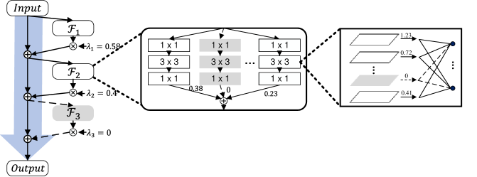
Figure 1: The network architecture of our method. ${\mathcal{F}}$ represents a residual function. Gray block, group and neuron mean they are inactive and can be pruned since their corresponding scaling factors are $0$.

3.1 Sparse Structure Selection

Given a training set consisting of $N$ sample-label pairs $\{{\bf x}_{i},{\bf y}_{i}\}_{1\leq i\leq N}$, then a $L$ layers CNN can be represented as a function ${\mathcal{C}}({\bf x}_{i},{\bf W})$, where ${\bf W}=\{{\bf W}^{l}\}_{1\leq l\leq L}$ represents the collection of all weights in the CNN. ${\bf W}$ is learned through solving an optimization problem of the form:

$$\min_{\bf W}{\frac{1}{N}\sum_{i=1}^{N}{{\mathcal{L}}({\bf y}_{i},{\mathcal{C}}({\bf x}_{i},{\bf W}))}+{\mathcal{R}}({\bf W})},$$ (1)

where ${\mathcal{L}}({\bf y}_{i},{\mathcal{C}}({\bf x}_{i},{\bf W}))$ is the loss on the sample ${\bf x}_{i}$, ${\mathcal{R}}(\cdot)$ is a non-structured regularization applying on every weight, e.g. $l_{2}$-norm as weight decay.

Prior sparse based model structure learning work [50, 1] tried to learn the number of neurons in a CNN. To achieve this goal, they added group sparsity regularization ${\mathcal{R}}_{g}(\cdot)$ on ${\bf W}^{l}_{k}$ into Eqn.1, and enforced entire ${\bf W}^{l}_{k}$ to zero during training. Another concurrent work by Wen et al. [43] adopted similar method but on multiple different structures. These ideas are straightforward but the implementations are nontrivial. First, the optimization is difficult since there are several constraints on weights simultaneously, including weight decay and group sparsity. Improper optimization technique may result in slow convergence and inferior results. Consequently, there is no successful attempt to directly apply these methods on large scale applications with complicated modern network architectures.

In this paper, we address structure learning problem in a more simple and effective way. Different from directly pushing weights in the same group to zero, we try to enforce the output of the group to zero. To achieve this goal, we introduce a new type of parameter – scaling factor $\lambda$ to scale the outputs of some specific structures (neurons, groups or blocks), and add sparsity constraint on $\lambda$ during training. Our goal is to obtain a sparse $\lambda$. Namely, if $\lambda^{i}=0$, then we can safely remove the corresponding structure since its outputs have no contribution to subsequent computation. Fig. 1 illustrates our framework.

Formally, the objective function of our proposed method can be formulated as:

$$\min_{{\bf W},\mbox{\boldmath$\lambda$\unboldmath}}{\frac{1}{N}\sum_{i=1}^{N}{{\mathcal{L}}({\bf y}_{i},{\mathcal{C}}({\bf x}_{i},{\bf W},\mbox{\boldmath$\lambda$\unboldmath}))}+{\mathcal{R}}({\bf W})+{\mathcal{R}}_{s}(\mbox{\boldmath$\lambda$\unboldmath})},$$ (2)

where ${\mathcal{R}}_{s}(\cdot)$ is a sparsity regularization for $\lambda$ with weight $\gamma$. In this work, we consider its most commonly used convex relaxation $l_{1}$-norm, which defined as $\gamma\|\mbox{\boldmath$\lambda$\unboldmath}\|_{1}$.

For ${\bf W}$, we can update it by Stochastic Gradient Descent (SGD) with momentum or its variants. For $\lambda$, we adopt Accelerated Proximal Gradient (APG) [30] method to solve it. For better illustration, we shorten $\frac{1}{N}\sum_{i=1}^{N}{{\mathcal{L}}({\bf y}_{i},{\mathcal{C}}({\bf x}_{i},\mbox{\boldmath$\lambda$\unboldmath}))}$ as ${\mathcal{G}}(\mbox{\boldmath$\lambda$\unboldmath})$, and reformulate the optimization of $\lambda$ as:

$$\min_{\mbox{\boldmath$\lambda$\unboldmath}}{{\mathcal{G}}(\mbox{\boldmath$\lambda$\unboldmath})+{\mathcal{R}}_{s}(\mbox{\boldmath$\lambda$\unboldmath})}.$$ (3)

Then we can update $\lambda$ by APG:

$${\bf d}_{(t)} =\mbox{\boldmath$\lambda$\unboldmath}_{(t-1)}+\frac{t-2}{t+1}(\mbox{\boldmath$\lambda$\unboldmath}_{(t-1)}-\mbox{\boldmath$\lambda$\unboldmath}_{(t-2)})$$ (4)

$${\bf z}_{(t)} ={\bf d}_{(t)}-\eta_{(t)}\nabla{\mathcal{G}}({\bf d}_{(t)})$$ (5)

$$\mbox{\boldmath$\lambda$\unboldmath}_{(t)} =\operatorname{\mathbf{prox}}_{\eta_{(t)}{\mathcal{R}}_{s}}({\bf z}_{(t)}),$$ (6)

where $\eta_{(t)}$ is gradient step size at iteration $t$ and $\operatorname{\mathbf{prox}}_{\eta{\mathcal{R}}_{s}}(\cdot)={\mathcal{S}}_{\eta\gamma}(\cdot)$ since ${\mathcal{R}}_{s}(\mbox{\boldmath$\lambda$\unboldmath})=\gamma\|\mbox{\boldmath$\lambda$\unboldmath}\|_{1}$. However, this formulation is not friendly for deep learning since additional to the pass for updating ${\bf W}$, we need to obtain $\nabla{\mathcal{G}}({\bf d}_{(t)})$ by extra forward-backward computation, which is computational expensive for deep neural networks. Thus, following the derivation in [40], we reformulate APG as a momentum based method:

$${\bf z}_{(t)} =\mbox{\boldmath$\lambda$\unboldmath}_{(t-1)}+\mu_{(t-1)}{\bf v}_{(t-1)}$$

$$~{}~{}~{}~{}-\eta_{(t)}\nabla{\mathcal{G}}(\mbox{\boldmath$\lambda$\unboldmath}_{(t-1)}+\mu_{(t-1)}{\bf v}_{(t-1)})$$ (7)

$${\bf v}_{(t)} ={\mathcal{S}}_{\eta_{(t)}\gamma}({\bf z}_{(t)})-\mbox{\boldmath$\lambda$\unboldmath}_{(t-1)}$$ (8)

$$\mbox{\boldmath$\lambda$\unboldmath}_{(t)} =\mbox{\boldmath$\lambda$\unboldmath}_{(t-1)}+{\bf v}_{(t)},$$ (9)

where we define ${\bf v}_{(t-1)}=\mbox{\boldmath$\lambda$\unboldmath}_{(t-1)}-\mbox{\boldmath$\lambda$\unboldmath}_{(t-2)}$ and $\mu_{(t-1)}=\frac{t-2}{t+1}$. This formulation is similar as the modified Nesterov Accelerated Gradient (NAG) in [40] except the update of ${\bf v}_{t}$. Furthermore, we simplified the update of $\lambda$ by replacing $\mbox{\boldmath$\lambda$\unboldmath}_{(t-1)}$ as $\mbox{\boldmath$\lambda$\unboldmath}^{\prime}_{(t-1)}=\mbox{\boldmath$\lambda$\unboldmath}_{(t-1)}+\mu_{(t-1)}{\bf v}_{(t-1)}$ following the modification of NAG in [4] which has been widely used in practical deep learning frameworks [5]. Our new parameters $\mbox{\boldmath$\lambda$\unboldmath}^{\prime}_{t}$ updates become:

$${\bf z}_{(t)} =\mbox{\boldmath$\lambda$\unboldmath}^{\prime}_{(t-1)}-\eta_{(t)}\nabla{\mathcal{G}}(\mbox{\boldmath$\lambda$\unboldmath}^{\prime}_{(t-1)})$$ (10)

$${\bf v}_{(t)} ={\mathcal{S}}_{\eta_{(t)}\gamma}({\bf z}_{(t)})-\mbox{\boldmath$\lambda$\unboldmath}^{\prime}_{(t-1)}+\mu_{(t-1)}{\bf v}_{(t-1)}$$ (11)

$$\mbox{\boldmath$\lambda$\unboldmath}^{\prime}_{(t)} ={\mathcal{S}}_{\eta_{(t)}\gamma}({\bf z}_{(t)})+\mu_{(t)}{\bf v}_{(t)}$$ (12)

In practice, we follow a stochastic approach with mini-batches and set momentum $\mu$ fixed to a constant value. Both ${\bf W}$ and $\lambda$ are updated in each iteration.

The implementation of APG is very simple and effective after our modification. In the following, we show it can be implemented by only ten lines of code in MXNet [5].


MXNet implementation of APG

import mxnet as mx
def apg_updater(weight, lr, grad, mom, gamma):
    z = weight - lr * grad
    z = soft_thresholding(z, lr * gamma)
    mom[:] = z - weight + 0.9 * mom
    weight[:] = z + 0.9 * mom
def soft_thresholding(x, gamma):
    y = mx.nd.maximum(0, mx.nd.abs(x) - gamma)
    return mx.nd.sign(x) * y

In our framework, we add scaling factors to three different CNN micro-structures, including neurons, groups and blocks to yield flexible structure selection. We will introduce these three cases in the following. Note that for networks with BN, we add scaling factors after BN to prevent the influence of bias parameters.

3.2 Neuron Selection

We introduce scaling factors for the output of channels to prune neurons. After training, removing the filters with zero scaling factor will result in a more compact network. A recent work proposed by Liu et al. [26] adopted similar idea for network slimming. They absorbed the scaling parameters into the parameters of batch normalization, and solve the optimization by subgradient descent. During training, scaling parameters whose absolute value are lower than a threshold value are set to 0. Comparing with [26], our method is more general and effective. Firstly, introducing scaling factor is more universal than reusing BN parameters. On one hand, some networks have no batch normalization layers, such as AlexNet [22] and VGG [37]; On the other hand, when we fine-tune pre-trained models on object detection or semantic segmentation tasks, the parameters of batch normalization are usually fixed due to small batch size. Secondly, the optimization of [26] is heuristic and need iterative pruning and retraining. In contrast, our optimization is more stable in an end-to-end manner. Above all, [26] can be seen as a special case of our method. Similarly, [48] is also a special case of our method. The difference between Ye et al. [48] and Liu et al. [26] is Ye et al. adopted ISTA [3] to optimize scaling factors. We will compare these different optimization methods in our experiments.

3.3 Block Selection

The structure of skip connection CNNs allows us to skip the computation of specific layers without cutting off the information flow in the network. Through stacking residual blocks, ResNet [11, 12] can easily exploit the advantage of very deep networks. Formally, residual block with identity mapping can be formulated by the following formula:

$${\bf r}^{i+1}={\bf r}^{i}+{\mathcal{F}}^{i}({\bf r}^{i},{\bf W}^{i}),$$ (13)

where ${\bf r}^{i}$ and ${\bf r}^{i+1}$ are input and output of the $i$-th block, ${\mathcal{F}}^{i}$ is a residual function and ${\bf W}^{i}$ are parameters of the block.

To prune blocks, we add scaling factor after each residual block. Then in our framework, the formulation of Eqn.13 is as follows:

$${\bf r}^{i+1}={\bf r}^{i}+\lambda^{i}{\mathcal{F}}^{i}({\bf r}^{i},{\bf W}^{i}).$$ (14)

As shown in Fig 1, after optimization, we can get a sparse $\lambda$. The residual block with scaling factor 0 will be pruned entirely, and we can learn a much shallower ResNet. A prior work that also adds scaling factors for residual in ResNet is Weighted Residual Networks [36]. Though sharing a lot of similarities, the motivations behind these two works are different. Their work focuses on how to train ultra deep ResNet to get better results with the help of scaling factors. Particularly, they increase depth from 100+ to 1000+. While our method aims to decrease the depth of ResNet, we use the scaling factors and sparse regularizations to sparsify the output of residual blocks.

3.4 Group Selection

Recently, Xie et al. introduced a new dimension – cardinality into ResNets and proposed ResNeXt [47]. Formally, they presented aggregated transformations as:

$${\mathcal{A}}({\bf x})=\sum_{i=1}^{C}{\mathcal{T}}^{i}({\bf x},{\bf W}^{i}),$$ (15)

where ${\mathcal{T}}^{i}({\bf x})$ represents a transformation with parameters ${\bf W}^{i}$, $C$ is the cardinality of the set of ${\mathcal{T}}^{i}({\bf x})$ to be aggregated. In practice, they use grouped convolution to ease the implementation of aggregated transformations. So in our framework, we refer $C$ as the number of group, and formulate a weighted ${\mathcal{A}}({\bf x})$ as:

$${\mathcal{A}}({\bf x})=\sum_{i=1}^{C}\lambda^{i}{\mathcal{T}}^{i}({\bf x},{\bf W}^{i})$$ (16)

After training, several basic cardinalities are chosen by a sparse $\lambda$ to form the final transformations. Then, the inactive groups with zero scaling factors can be safely removed as shown in Fig 1. Note that neuron pruning can also seen as a special case of group pruning when each group contains only one neuron. Furthermore, we can combine block pruning and group pruning to learn more flexible network structures.

4 Experiments

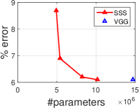
(a) VGG CIFAR10

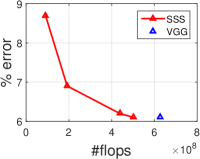
(b) VGG CIFAR10

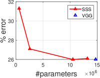
(c) VGG CIFAR100

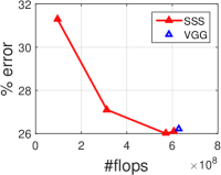
(d) VGG CIFAR100

Figure 2: Error vs. number of parameters and FLOPs after SSS training for VGG on CIFAR-10 and CIFAR-100 datasets.

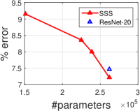
(a) ResNet20 CIFAR10

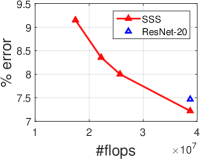
(b) ResNet20 CIFAR10

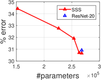
(c) ResNet20 CIFAR100

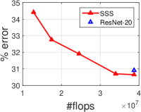
(d) ResNet20 CIFAR100

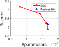
(e) ResNet164 CIFAR10

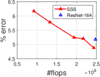
(f) ResNet164 CIFAR10

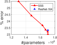
(g) ResNet164 CIFAR100

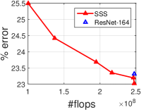
(h) ResNet164 CIFAR100

Figure 3: Error vs. number of parameters and FLOPs after SSS training for ResNet-20 and ResNet-164 on CIFAR-10 and CIFAR-100 datasets.

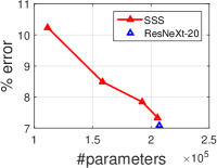
(a) ResNeXt20 CIFAR10

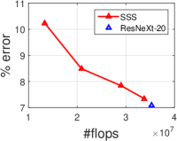
(b) ResNeXt20 CIFAR10

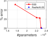
(c) ResNeXt20 CIFAR100

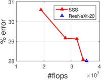
(d) ResNeXt20 CIFAR100

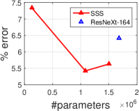
(e) ResNeXt164 CIFAR10

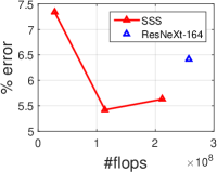
(f) ResNeXt164 CIFAR10

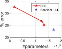
(g) ResNeXt164 CIFAR100

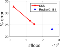
(h) ResNeXt164 CIFAR100

Figure 4: Error vs. number of parameters and FLOPs with SSS training for ResNeXt-20 and ResNeXt-164 on CIFAR-10 and CIFAR-100 datasets.

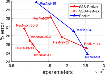
(a) Parameters

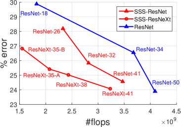
(b) FLOPs

Figure 5: Top-1 error vs. number of parameters and FLOPs for our SSS models and original ResNets on ImageNet validation set.

In this section, we evaluate the effectiveness of our method on three standard datasets, including CIFAR-10, CIFAR-100 [21] and ImageNet LSVRC 2012 [34]. For neuron pruning, we adopt VGG16 [37], a classical plain network to validate our method. As for blocks and groups, we use two state-of-the-art networks, ResNet [12] and ResNeXt [47] respectively. To prove the practicability of our method, we further experiment in a very lightweight network, PeleeNet [42].

For optimization, we adopt NAG [40, 4] and our modified APG to update weights ${\bf W}$ and scaling factors $\lambda$, respectively. We set weight decay of ${\bf W}$ to 0.0001 and fix momentum to 0.9 for both ${\bf W}$ and $\lambda$. The weights are initialized as in [11] and all scaling factors are initialized to be 1. All the experiments are conducted in MXNet [5].

4.1 CIFAR

We start with CIFAR dataset to evaluate our method. CIFAR-10 dataset consists of 50K training and 10K testing RGB images with 10 classes. CIFAR-100 is similar to CIFAR-10, except it has 100 classes. As suggested in [11], the input image is $32\times 32$ randomly cropped from a zero-padded $40\times 40$ image or its flipping. The models in our experiments are trained with a mini-batch size of 64 on a single GPU. We start from a learning rate of 0.1 and train the models for 240 epochs. The learning rate is divided by 10 at the 120-th,160-th and 200-th epoch.

VGG: The baseline network is a modified VGG16 with BN [19]. We remove fc6 and fc7 and only use one fully-connected layer for classification. We add scale factors after every batch normalization layers. Fig. 2 shows the results of our method. Both parameters and floating-point operations per second (FLOPs) are reported. Our method can save about 30% parameters and 30% - 50% computational cost with minor lost of performance.

ResNet: To learn the number of residual blocks, we use ResNet-20 and ResNet-164 [12] as our baseline networks. ResNet-20 consists of 9 residual blocks. Each block has 2 convolutional layers, while ResNet-164 has 54 blocks with bottleneck structure in each block. Fig. 3 summarizes our results. It is easy to see that our SSS achieves better performance than the baseline model with similar parameters and FLOPs. For ResNet-164, our SSS yields 2.5x speedup with about $2\%$ performance loss both in CIFAR-10 and CIFAR-100. After optimization, we found that the blocks in early stages are pruned first. This discovery coincides with the common design that the network should spend more budget in its later stage, since more and more diverse and complicated pattern may emerge as the receptive field increases.

Table 1: Network architectures of ResNet-50 and our pruned ResNets for ImageNet. $\surd$ represents that the corresponding block is kept while $\times$ denotes that the block is pruned

stage	output	ResNet-50	ResNet-26	ResNet-32	ResNet-41
conv1	112$\times$112	7$\times$7, 64, stride 2
conv2	56$\times$56	3$\times$3 max pool, stride 2
		$\begin{bmatrix}\text{1}\times\text{1},\text{64}~{}~{}\\ \text{3}\times\text{3},\text{64}~{}~{}\\ \text{1}\times\text{1},\text{256}\end{bmatrix}\times\text{3}$	$\times\times\times$	$\times\times\surd$	$\times\times\times$
conv3	28$\times$28	$\begin{bmatrix}\text{1}\times\text{1},\text{128}~{}~{}\\ \text{3}\times\text{3},\text{128}~{}~{}\\ \text{1}\times\text{1},\text{512}~{}~{}\end{bmatrix}\times\text{4}$	$\times\surd\surd\times$	$\surd\surd\surd\surd$	$\surd\surd\surd\surd$
conv4	14$\times$14	$\begin{bmatrix}\text{1}\times\text{1},\text{256}~{}~{}\\ \text{3}\times\text{3},\text{256}~{}~{}\\ \text{1}\times\text{1},\text{1024}\end{bmatrix}\times\text{6}$	$\times\surd\surd\surd\surd\surd$	$\surd\surd\surd\times\times\surd$	$\surd\surd\surd\surd\surd\surd$
conv5	7$\times$7	$\begin{bmatrix}\text{1}\times\text{1},\text{512}~{}~{}\\ \text{3}\times\text{3},\text{512}~{}~{}\\ \text{1}\times\text{1},\text{2048}\end{bmatrix}\times\text{3}$	$\surd\times\times$	$\surd\times\times$	$\surd\surd\surd$
	1$\times$1	global average pool 1000-d FC, softmax

ResNeXt: We also test our method on ResNeXt [47]. We choose ResNeXt-20 and ResNeXt-164 as our base networks. Both of these two networks have bottleneck structures with 32 groups in residual blocks. For ResNeXt-20, we focus on groups pruning since there are only 6 residual blocks in it. For ResNeXt-164, we add sparsity on both groups and blocks. Fig. 4 shows our experiment results. Both groups pruning and block pruning show good trade-off between parameters and performance, especially in ResNeXt-164. The combination of groups and blocks pruning is extremely effective in CIFAR-10. Our SSS saves about $60\%$ FLOPs while achieves $1\%$ higher accuracy. In ResNeXt-20, groups in first and second block are pruned first. Similarly, in ResNeXt-164, groups in shallow residual blocks are pruned mostly.

Table 2: Results on ImageNet dataset. Both top-1 and top-5 validation errors (single crop) are reported. Number of parameters and FLOPs for inference of different models are also shown. Here, M/B means million/billion ($10^{6}/10^{9}$), respectively

Model	Top-1	Top-5	#Parameters	#FLOPs
VGG-16	27.54	9.16	138.3M	30.97B
VGG-16	31.47	11.8	130.5M	7.667B
ResNet-50	23.88	7.14	25.5M	4.089B
ResNet-41	24.56	7.39	25.3M	3.473B
ResNet-32	25.82	8.09	18.6M	2.818B
ResNet-26	28.18	9.21	15.6M	2.329B
ResNeXt-50	22.43	6.32	25.0M	4.230B
ResNeXt-41	24.07	7.00	12.4M	3.234B
ResNeXt-38	25.02	7.50	10.7M	2.431B
ResNeXt-35-A	25.43	7.83	10.0M	2.068B
ResNeXt-35-B	26.83	8.42	8.50M	1.549B

4.2 ImageNet LSVRC 2012

To further demonstrate the effectiveness of our method in large-scale CNNs, we conduct more experiments on the ImageNet LSVRC 2012 classification task with VGG16 [37], ResNet-50 [12] and ResNeXt-50 (32 $\times$ 4d) [47]. We do data augmentation based on the publicly available implementation of “fb.resnet” . The mini-batch size is 128 on 4 GPUs for VGG16 and ResNet-50, and 256 on 8 GPUs for ResNeXt-50. The optimization and initialization are similar as those in CIFAR experiments. We train the models for 100 epochs. The learning rate is set to an initial value of 0.1 and then divided by 10 at the 30-th, 60-th and 90-th epoch. All the results for ImageNet dataset are summarized in Table 2.

VGG16: In our experiments of VGG16 pruning, we find the results of pruning all convolutional layers were not promising. This is because in VGG16, the computational cost in terms of FLOPs is not equally distributed in each layer. The number of FLOPs of conv5 layers is 2.77 billion in total, which is only 9% of the whole network (30.97 billion). Thus, we consider the sparse penalty should be adjusted by computational cost of different layers. Similar idea has been adopted in [29] and [13]. In [29], they introduce FLOPs regularization to the pruning criteria. He et al. [13] do not prune conv5 layers in their VGG16 experiments. Following [13], we set the sparse penalty of conv5 to 0 and only prune conv1 to conv4. The results can be found in Table 2. The pruned model save about 75% FLOPs, while the parameter saving is negligible. This is due to that fully-connected layers have a large amount of parameters (123 million in original VGG16), and we do not pruned fully-connected layers for fair comparison with other methods.

ResNet-50: For ResNet-50, we experiment three different settings of $\gamma$ to explore the performance of our method in block pruning. For simplicity, we denote the trained models as ResNet-26, ResNet-32 and ResNet-41 depending on their depths. Their structures are shown in Table 1. All the pruned models come with accuracy loss in certain extent. Comparing with original ResNet-50, ResNet-41 provides $15\%$ FLOPs reduction with $0.7\%$ top-1 accuracy loss while ResNet-32 saves $31\%$ FLOPs with about $2\%$ top-1 loss. Fig. 5 shows the top-1 validation errors of our SSS models and ResNets as a function of the number of parameters and FLOPs. The results reveal that our pruned models perform on par with original hand-crafted ResNets, whilst requiring less parameters and computational cost. For example, comparing with ResNet-34 [12], both our ResNet-41 and ResNet-32 yield better performances with less FLOPs.

ResNeXt-50: As for ResNeXt-50, we add sparsity constraint on both residual blocks and groups which results in several pruned models. Table 2 summarizes the performance of these models. The learned ResNeXt-41 yields $24\%$ top-1 error in ILSVRC validation set. It gets similar results with the original ResNet50, but with half parameters and more than 20% less FLOPs. In ResNeXt-41, three residual blocks in “conv5” stage are pruned entirely. This pruning result is somewhat contradict to the common design of CNNs, which worth to be studied in depth in the future.

4.3 Pruning lightweight network

Adopting lightweight networks, such as MobileNet[15], ShuffleNet[45] for fast inference is a more effective strategy in practice. To future prove the effectiveness of our method, we adopt neuron pruning in PeleeNet[42], which is a state-of-the-art efficient architecture without separable convolution. We follow the training settings and hyper-parameters used in [45]. The mini-batch size is 1024 on 8 GPUs and we train 240 epoch. Table 3 shows the pruning results of PeleeNet. We adopt different settings of $\gamma$ and get three pruned networks. Comparing to baseline, Our purned PeleeNet-A save about 14% parameters and FLOPs with only 0.4% top-1 accuracy degradation.

Table 3: Results of PeleeNet on ImageNet dataset

Model	Top-1	Top-5	#Parameters	#FLOPs
PeleeNet (Our impl.)	27.47	9.15	2.8M	508M
PeleeNet-A	27.85	9.34	2.4M	436M
PeleeNet-B	30.87	11.38	1.6M	293M
PeleeNet-C	32.81	12.69	1.4M	236M

4.4 Comparison with other methods

We compare our SSS with other pruning methods, including SSL [43], filter pruning [24], channel pruning [13], ThiNet [27], [29] and [48]. We compare SSL with our method in CIFAR10 and CIFAR100. All the models are trained from scratch. As shown in Fig. 6, our SSS achieves much better performances than SSL, even SSL with finetune. Table 4 shows the pruning results on the ImageNet LSVRC2012 dataset. To the best of our knowledge, only a few works reported ResNet pruning results with FLOPs. Comparing with filter pruning results, our ResNet-32 performs best with least FLOPs. As for channel pruning, with similar FLOPs, our ResNet-32 yields 1.88% lower top-1 error and 1.11% lower top-5 error than pruned ResNet-50 provided by [13]. As for [48], our ResNet-41 achieves about 1% lower top-1 error with less computation budge. We also show comparison in VGG16. All the method including channel pruning, ThiNet and our SSS achieve significant improvement than [29]. Our VGG16 pruning result is competitive to other state-of-the-art.

We further compare our pruned ResNeXt with DenseNet [17] in Table 5. With 14% less FLOPs, Our ResNeXt-38 achieves 0.2% lower top-5 error than DenseNet-121.

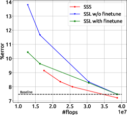
(a) CIFAR10

(b) CIFAR100

Figure 6: Error vs. FLOPs for our SSS models and SSL models

Table 4: Comparison among several state-of-the-art pruning methods on the ResNet and VGG16 networks

Model	Top-1	Top-5	#FLOPs
ResNet-34-pruned [24]	27.44	-	3.080B
ResNet-50-pruned-A [24] (Our impl.)	27.12	8.95	3.070B
ResNet-50-pruned-B [24] (Our impl.)	27.02	8.92	3.400B
ResNet-50-pruned (2$\times$) [13]	27.70	9.20	2.726B
ResNet-32 (Ours)	25.82	8.09	2.818B
ResNet-101-pruned [48]	25.44	-	3.690B
ResNet-41 (Ours)	24.56	7.39	3.473B
VGG16-pruned [29]	-	15.5	$\approx$8.0B
VGG16-pruned (5$\times$) [13]	32.20	11.90	7.033B
VGG16-pruned (ThiNet-Conv) [27]	30.20	10.47	9.580B
VGG16-pruned (Ours)	31.47	11.80	7.667B

Table 5: Comparison between pruned ResNeXt-38 and DenseNet-121

Model	Top-1	Top-5	#FLOPs
DenseNet-121 [17]	25.02	7.71	2.834B
DenseNet-121 [17] (Our impl.)	25.58	7.89	2.834B
ResNeXt-38 (Ours)	25.02	7.50	2.431B

4.5 Choice of different optimization methods

We compare our APG with other different optimization methods for optimizing $\lambda$ in our ImageNet experiments, including SGD adopted in [26] and ISTA [3] used in [48]. We adopted ResNet-50 for block pruning and train it from scratch. The sparse penalty $\gamma$ is set to 0.005 for all optimization methods.

Table 6: Comparison between different optimization methods

Model	Top-1	Top-5	#FLOPs
ResNet-32-SGD	26.46	8.41	2.726B
ResNet-32-APG	25.82	7.39	2.818B

For SGD, since we can not get exact zero scale factor during training, a extra hyper-parameter – hard threshold is need for the optimization of $\lambda$. In our experiment, we set it to $0.0001$. After training, we get a ResNet-32-SGD network. As show in Table 6, the performance of our ResNet-32-APG is better than ResNet-32-SGD.

For ISTA, we found the optimization of network could not converge. The reason is that the converge speed of ISTA for $\lambda$ optimization is too slow when training from scratch. Adopting ISTA can get reasonable results in CIFAR dataset. However, in ImageNet, it is hard to optimize the $\lambda$ to be sparse with small $\gamma$, and larger $\gamma$ will lead too many zeros in our experiments. [48] alleviated this problem by fine-tunning from a pretrained model. They also adopted $\lambda$-${\bf W}$ rescaling trick to get an small $\lambda$ initialization.

Comparing to ISTA, Our APG can be seen as a modified version of an improved ISTA, namely FISTA [3], which has been proved to be significantly better than ISTA in convergence. Thus the optimization of our method is effective and stable in both CIFAR and ImageNet experiments. The results described in Table 4 also show the advantages of our APG method to ISTA. The performance of our trained ResNet-41 is better than ResNet-101-pruned provided by [48].

5 Conclusions

In this paper, we have proposed a data-driven method, Sparse Structure Selection (SSS) to adaptively learn the structure of CNNs. In our framework, the training and pruning of CNNs is formulated as a joint sparse regularized optimization problem. Through pushing the scaling factors which are introduced to scale the outputs of specific structures to zero, our method can remove the structures corresponding to zero scaling factors. To solve this challenging optimization problem and adapt it into deep learning models, we modified the Accelerated Proximal Gradient method. In our experiments, we demonstrate very promising pruning results on PeleeNet, VGG, ResNet and ResNeXt. We can adaptively adjust the depth and width of these CNNs based on budgets at hand and difficulties of each task. We believe these pruning results can further inspire the design of more compact CNNs.

In future work, we plan to apply our method in more applications such as object detection. It is also interesting to investigate the use of more advanced sparse regularizers such as non-convex relaxations, and adjust the penalty based on the complexity of different structures adaptively.

References

- [1] Alvarez, J.M., Salzmann, M.: Learning the number of neurons in deep networks. In: NIPS (2016)
- [2] Baker, B., Gupta, O., Naik, N., Raskar, R.: Designing neural network architectures using reinforcement learning. In: ICLR (2017)
- [3] Beck, A., Teboulle, M.: A fast iterative shrinkage-thresholding algorithm for linear inverse problems. SIAM journal on imaging sciences 2(1), 183–202 (2009)
- [4] Bengio, Y., Boulanger-Lewandowski, N., Pascanu, R.: Advances in optimizing recurrent networks. In: ICASSP (2013)
- [5] Chen, T., Li, M., Li, Y., Lin, M., Wang, N., Wang, M., Xiao, T., Xu, B., Zhang, C., Zhang, Z.: MXNet: A flexible and efficient machine learning library for heterogeneous distributed systems. In: NIPS Workshop (2015)
- [6] Courbariaux, M., Hubara, I., Soudry, D., El-Yaniv, R., Bengio, Y.: Binarized neural networks: Training deep neural networks with weights and activations constrained to +1 or -1. In: NIPS (2016)
- [7] Denton, E.L., Zaremba, W., Bruna, J., LeCun, Y., Fergus, R.: Exploiting linear structure within convolutional networks for efficient evaluation. In: NIPS (2014)
- [8] Guo, Y., Yao, A., Chen, Y.: Dynamic network surgery for efficient dnns. In: NIPS (2016)
- [9] Han, S., Pool, J., Tran, J., Dally, W.: Learning both weights and connections for efficient neural network. In: NIPS (2015)
- [10] Hassibi, B., Stork, D.G., et al.: Second order derivatives for network pruning: Optimal brain surgeon. In: NIPS (1993)
- [11] He, K., Zhang, X., Ren, S., Sun, J.: Deep residual learning for image recognition. In: CVPR (2016)
- [12] He, K., Zhang, X., Ren, S., Sun, J.: Identity mappings in deep residual networks. In: ECCV (2016)
- [13] He, Y., Zhang, X., Sun, J.: Channel pruning for accelerating very deep neural networks. In: ICCV (2017)
- [14] Hinton, G., Vinyals, O., Dean, J.: Distilling the knowledge in a neural network. In: NIPS Workshop (2014)
- [15] Howard, A.G., Zhu, M., Chen, B., Kalenichenko, D., Wang, W., Weyand, T., Andreetto, M., Adam, H.: Mobilenets: Efficient convolutional neural networks for mobile vision applications. arXiv preprint arXiv:1704.04861 (2017)
- [16] Hu, H., Peng, R., Tai, Y.W., Tang, C.K.: Network trimming: A data-driven neuron pruning approach towards efficient deep architectures. arXiv:1607.03250 (2016)
- [17] Huang, G., Liu, Z., Weinberger, K.Q., van der Maaten, L.: Densely connected convolutional networks. In: CVPR (2017)
- [18] Iandola, F.N., Han, S., Moskewicz, M.W., Ashraf, K., Dally, W.J., Keutzer, K.: Squeezenet: Alexnet-level accuracy with 50x fewer parameters and¡ 0.5 mb model size. arXiv:1602.07360 (2016)
- [19] Ioffe, S., Szegedy, C.: Batch normalization: Accelerating deep network training by reducing internal covariate shift. ICML (2015)
- [20] Jaderberg, M., Vedaldi, A., Zisserman, A.: Speeding up convolutional neural networks with low rank expansions. BMVC (2014)
- [21] Krizhevsky, A., Hinton, G.: Learning multiple layers of features from tiny images. Tech Report (2009)
- [22] Krizhevsky, A., Sutskever, I., Hinton, G.E.: ImageNet classification with deep convolutional neural networks. In: NIPS (2012)
- [23] LeCun, Y., Denker, J.S., Solla, S.A., Howard, R.E., Jackel, L.D.: Optimal brain damage. In: NIPS (1990)
- [24] Li, H., Kadav, A., Durdanovic, I., Samet, H., Graf, H.P.: Pruning filters for efficient ConvNets. In: ICLR (2017)
- [25] Liu, B., Wang, M., Foroosh, H., Tappen, M., Pensky, M.: Sparse convolutional neural networks. In: CVPR (2015)
- [26] Liu, Z., Li, J., Shen, Z., Huang, G., Yan, S., Zhang, C.: Learning efficient convolutional networks through network slimming. In: ICCV (2017)
- [27] Luo, J.H., Wu, J., Lin, W.: ThiNet: A filter level pruning method for deep neural network compression. In: ICCV (2017)
- [28] Mariet, Z., Sra, S.: Diversity networks. In: ICLR (2016)
- [29] Molchanov, P., Tyree, S., Karras, T., Aila, T., Kautz, J.: Pruning convolutional neural networks for resource efficient inference. In: ICLR (2017)
- [30] Parikh, N., Boyd, S., et al.: Proximal algorithms. Foundations and Trends® in Optimization 1(3), 127–239 (2014)
- [31] Rastegari, M., Ordonez, V., Redmon, J., Farhadi, A.: XNOR-Net: ImageNet classification using binary convolutional neural networks. In: ECCV (2016)
- [32] Real, E., Moore, S., Selle, A., Saxena, S., Suematsu, Y.L., Le, Q., Kurakin, A.: Large-scale evolution of image classifiers. In: ICML (2017)
- [33] Romero, A., Ballas, N., Kahou, S.E., Chassang, A., Gatta, C., Bengio, Y.: FitNets: Hints for thin deep nets. In: ICLR (2015)
- [34] Russakovsky, O., Deng, J., Su, H., Krause, J., Satheesh, S., Ma, S., Huang, Z., Karpathy, A., Khosla, A., Bernstein, M., et al.: ImageNet large scale visual recognition challenge. International Journal of Computer Vision 115(3), 211–252 (2015)
- [35] Sergey, Z., Nikos, K.: Paying more attention to attention: Improving the performance of convolutional neural networks via attention transfer. In: ICLR (2017)
- [36] Shen, F., Gan, R., Zeng, G.: Weighted residuals for very deep networks. In: ICSAI (2016)
- [37] Simonyan, K., Zisserman, A.: Very deep convolutional networks for large-scale image recognition. In: ICLR (2015)
- [38] Srinivas, S., Babu, R.V.: Learning neural network architectures using backpropagation. In: BMVC (2016)
- [39] Srivastava, R.K., Greff, K., Schmidhuber, J.: Highway networks. In: ICML (2015)
- [40] Sutskever, I., Martens, J., Dahl, G., Hinton, G.: On the importance of initialization and momentum in deep learning. In: ICML (2013)
- [41] Veit, A., Wilber, M.J., Belongie, S.: Residual networks behave like ensembles of relatively shallow networks. In: NIPS (2016)
- [42] Wang, R.J., Li, X., Ao, S., Ling, C.X.: Pelee: A real-time object detection system on mobile devices. In: ICLR Workshop (2018)
- [43] Wen, W., Wu, C., Wang, Y., Chen, Y., Li, H.: Learning structured sparsity in deep neural networks. In: NIPS (2016)
- [44] Wu, J., Leng, C., Wang, Y., Hu, Q., Cheng, J.: Quantized convolutional neural networks for mobile devices. In: CVPR (2016)
- [45] Xiangyu, Z., , Xinyu, Z., Mengxiao, L., Jian, S.: Shufflenet: An extremely efficient convolutional neural network for mobile devices. In: BMVC (2016)
- [46] Xie, L., Yuille, A.: Genetic CNN. In: ICCV (2017)
- [47] Xie, S., Girshick, R., Dollár, P., Tu, Z., He, K.: Aggregated residual transformations for deep neural networks. In: CVPR (2017)
- [48] Ye, J., Lu, X., Lin, Z., Wang, J.Z.: Rethinking the smaller-norm-less-informative assumption in channel pruning of convolution layers. In: ICLR (2018)
- [49] Zhang, X., Zou, J., Ming, X., He, K., Sun, J.: Efficient and accurate approximations of nonlinear convolutional networks. In: CVPR (2015)
- [50] Zhou, H., Alvarez, J.M., Porikli, F.: Less is more: Towards compact cnns. In: ECCV (2016)
- [51] Zoph, B., Le, Q.V.: Neural architecture search with reinforcement learning. In: ICLR (2017)