Abstract

This paper is concerned with the application of finite element methods to obtain solutions for steady fully developed second-grade flows in a curved pipe of circular cross-section and arbitrary curvature ratio, under a given axial pressure gradient. The qualitative and quantitative behavior of the secondary flows is analyzed with respect to inertia and viscoelasticity.

Key words. Second-grade fluid, curved pipe, fully developed flows, creeping viscoelastic flows, inertial viscoelastic flows, finite elements.

1 Introduction

Fully developed viscous flow in a curved pipe with circular cross-section was first studied theoretically by Dean ([11], [12]) applying regular perturbation methods. He showed that for small curvature ratio the flow depends only on a single parameter, the so-called Dean number. In [19], Soh and Berger solved the Navier-Stokes equations for the fully developed flow of an homogeneous Newtonian fluid in a curved pipe of circular cross-section for arbitrary curvature ratio. They solved numerically the Navier-Stokes system in the primitive variables form using a finite difference scheme. Closed form perturbation solutions for a second order model were obtained by several authors in the special case where the second normal stress coefficient is zero.

For this model, Jitchote and Robertson [17] obtained analytical solutions to the perturbation equations and analyze the effects of non-zero second normal stress coefficient on the behaviour of the solution. Theoretical results regarding this problem using a splitting method were obtained by Coscia and Robertson [10].

Our aim here is to apply the finite element method to the second-grade model for fully developped flows in a curved pipe and analyze the non-Newtonian effects of the flow. Quantitative and qualitative behaviour of the axial velocity and the stream function of creeping and inertial second-grade fluids are also studied. Similar techniques have been applied to other non-Newtonian models (see [3], [4]).

The paper is organized as follows. In Section $2$, we consider the governing equations and rewrite the problem in an equivalent decoupled form, composed of a Stokes-like system and a transport equation considered as two auxiliary linear problems. In order to describe the curved pipe geometry, these equations are presented in non-dimensional polar coordinates in Section $3$. In Section $4$, we outline tha discretization method using a finite element method to obtain approximate solutions to the original problem. Finally, numerical experiments based on a decoupled fixed point algorithm are illustrated in Section $5$. A systematic numerical study of the qualitative behaviour of inertial and viscoelastic effects for a certain range of non-dimensional parameters (Reynolds number, viscoelastic coefficient and pipe curvature) associated to the model is performed. The issue of increasing the values of the parameters for which the convergence of the proposed iterative algorithm can be shown, is addressed by using a continuation method.

2 Governing equations

We consider steady isothermal flows of incompressible second-grade fluids in a curved pipe $\Omega\subset{I~{}R}^{3}$ with boundary $\partial\Omega$, constant circular cross–section $\Omega_{S}$ of radius $r$ with the line of centers coiled in a circle of radius $R$ (see Figure 1).

Figure 1: Polar toroidal coordinates in a curved pipe.

The corresponding equations are given by

$$\left\{\!\!\begin{array}[]{ll}-\mu\Delta\mathbf{u}-\widetilde{\alpha}_{1}\mathbf{u}\cdot\!\nabla\Delta\mathbf{u}+\!\rho\mathbf{u}\cdot\!\nabla\mathbf{u}+\nabla\pi\!=\!\nabla\!\cdot\widetilde{\mathbf{L}}(\mathbf{u})&\text{ in }\Omega,\vspace{2mm}\\ \nabla\!\cdot\mathbf{u}=0&\text{ in }\Omega,\vspace{2mm}\\ \mathbf{u}=0&\text{ on }\partial\Omega,\end{array}\right.$$

where $\mathbf{u}$ is the fluid velocity, $\pi$ is the pressure, $\mu$ is the viscosity, $\rho$ is the constant density, $\widetilde{\alpha}_{1}$ and $\widetilde{\alpha}_{2}$ are the Rivlin-Ericksen material constants, and $\widetilde{\mathbf{L}}(\mathbf{u})$ is a nonlinear term given by

$$\widetilde{\mathbf{L}}(\mathbf{u})\!=\!\widetilde{\alpha}_{1}\nabla\mathbf{u}^{T}\!\left(\nabla\mathbf{u}+\nabla\mathbf{u}^{T}\right)+(\widetilde{\alpha}_{1}+\widetilde{\alpha}_{2})\!\left(\nabla\mathbf{u}+\nabla\mathbf{u}^{T}\right)^{2}.$$

We consider an adimensionalised formulation of the previous system by introducing the following quantities

$$\mathbf{x}=\textstyle\tfrac{\widetilde{\mathbf{x}}}{a},\qquad\mathbf{u}=\tfrac{\widetilde{\mathbf{u}}}{U},\qquad\pi=\tfrac{\widetilde{\pi}a}{\mu U},$$ (1)

where the symbol $\ \widetilde{}\$ is attached to dimensional parameters ($U$ represents a characteristic velocity of the flow). We also introduce the Reynolds number $\mathcal{R}e$ and two non–dimensional ratios involving the constant material moduli $\widetilde{\alpha}$ and $\widetilde{\alpha}_{2}$,

$$\mathcal{R}e=\textstyle\tfrac{\rho Ua}{\mu},\qquad\alpha_{1}=\textstyle\tfrac{U\widetilde{\alpha}}{\mu a},\qquad\alpha_{2}=\textstyle\tfrac{U\widetilde{\alpha}_{2}}{\mu a}.$$

The dimensionless system takes the form

$$\left\{\!\!\begin{array}[c]{ll}-\Delta\mathbf{u}-\alpha_{1}\mathbf{u}\cdot\!\nabla\Delta\mathbf{u}+{\mathcal{R}}e\,\mathbf{u}\cdot\!\nabla\mathbf{u}+\nabla\pi\!=\!\nabla\!\cdot\mathbf{L}(\mathbf{u})&\text{ in }\Omega,\vspace{2mm}\\ \nabla\!\cdot\mathbf{u}=0&\text{ in }\Omega,\vspace{2mm}\\ \mathbf{u}=0&\text{ on }\partial\Omega,\end{array}\right.$$ (2)

with

$$\mathbf{L}(\mathbf{u})\!=\!\alpha_{1}\nabla\mathbf{u}^{T}\!\big{(}\nabla\mathbf{u}+\nabla\mathbf{u}^{T}\big{)}+(\alpha_{1}+\alpha_{2})\!\big{(}\nabla\mathbf{u}+\nabla\mathbf{u}^{T}\big{)}^{2}.$$

System (2) can be rewritten in the following equivalent form involving a Stokes system and a transport equation,

$$\left\{\!\!\begin{array}[c]{ll}-\Delta\mathbf{u}+\nabla p=\boldsymbol{\varrho}&\text{ in }\Omega,\vspace{2mm}\\ \nabla\cdot\mathbf{u}=0&\text{ in }\Omega,\vspace{2mm}\\ \mathbf{u}=0&\text{ on }\partial\Omega,\vspace{2mm}\\ \boldsymbol{\varrho}\!+\!\alpha_{1}\mathbf{u}\cdot\!\nabla\boldsymbol{\varrho}\!=\!\nabla\!\cdot\!\left(\mathbf{L}(\mathbf{u})\!-\!{\cal R}e\,\mathbf{u}\otimes\mathbf{u}\!-\!\alpha_{1}p\nabla\!\mathbf{u}^{T}\right)&\text{ in }\Omega,\end{array}\right.$$ (3)

where the new variable $p$ is given by $\pi\!=\!p\!+\!\alpha_{1}\mathbf{u}\cdot\!\nabla p$. In the following lemma, we (formally) prove that if $\mathbf{u}$ is such that the operator $I+\alpha_{1}\mathbf{u}\cdot\nabla$ is invertible, then problems (2) and (3) are equivalent.

Lemma 1

If $(\mathbf{u},p,\varrho)$ is a strong solution of $(\ref{couplestcurved})$, then $(\mathbf{u},p+\alpha\mathbf{u}\cdot\nabla p)$ is a strong solution of $(\ref{ssfcurved})$. Conversely, if $(\mathbf{u},\pi)$ is a strong solution for $(\ref{ssfcurved})$ and if $I+\alpha_{1}\mathbf{u}\cdot\nabla$ is invertible, then $(\mathbf{u},(I+\alpha_{1}\mathbf{u}\cdot\nabla)^{-1}\pi,\boldsymbol{\varrho})$ is a solution of $(\ref{couplestcurved})$.

Proof. Let $(\mathbf{u},p,\boldsymbol{\varrho})$ be a solution of (3). Applying the operator $I+\alpha_{1}\mathbf{u}\cdot\nabla$ to both sides of $(\ref{couplestcurved})_{1}$, and taking into account $(\ref{couplestcurved})_{2}$-$(\ref{couplestcurved})_{4}$, we obtain

$$\begin{array}[]{ll}\big{(}I+\alpha_{1}\mathbf{u}\cdot\nabla\big{)}\big{(}\Delta\mathbf{u}+\nabla p\big{)}=\big{(}I+\alpha_{1}\mathbf{u}\cdot\nabla\big{)}\boldsymbol{\varrho}\vspace{2mm}\\ =\nabla\cdot\big{(}\mathbf{L}(\mathbf{u})-{\cal R}e\,\mathbf{u}\otimes\mathbf{u}-\alpha_{1}p\left(\nabla\mathbf{u}\right)^{T}\big{)}\vspace{2mm}\\ =\nabla\cdot\mathbf{L}(\mathbf{u})-{\cal R}e\,\mathbf{u}\cdot\nabla\mathbf{u}-\alpha_{1}\nabla\big{(}\mathbf{u}\cdot\nabla p\big{)}+\alpha_{1}\nabla\cdot\big{(}\nabla p\otimes\mathbf{u}\big{)}\vspace{2mm}\\ =\nabla\cdot\mathbf{L}(\mathbf{u})-{\cal R}e\,\mathbf{u}\cdot\nabla\mathbf{u}-\alpha_{1}\nabla\big{(}\mathbf{u}\cdot\nabla p\big{)}+\alpha_{1}\mathbf{u}\cdot\nabla(\nabla p)\vspace{2mm}\\ =\nabla\cdot\mathbf{L}(\mathbf{u})-{\cal R}e\,\mathbf{u}\cdot\nabla\mathbf{u}-\nabla\big{(}p+\alpha_{1}\mathbf{u}\cdot\nabla p\big{)}+\big{(}I+\alpha_{1}\mathbf{u}\cdot\nabla\big{)}\nabla p.\end{array}$$

Setting $\pi=p+\alpha_{1}\mathbf{u}\cdot\nabla p$ we easily see that $(\mathbf{u},\pi)$ is a solution of $(\ref{ssfcurved})$. Conversely, let $(\mathbf{u},\pi)$ be a solution of (2). From $(\ref{ssfcurved})_{1}$, it follows that

$$-\left(I+\alpha_{1}\mathbf{u}\cdot\nabla\right)\,\Delta\mathbf{u}+{\cal R}e\ \mathbf{u}\cdot\nabla\mathbf{u}+\nabla\pi=\nabla\cdot\mathbf{L}(\mathbf{u}).$$

This equation together with the fact that

$$\big{(}I+\alpha_{1}\mathbf{u}\cdot\nabla\big{)}\nabla p-\nabla\pi=-\alpha_{1}\nabla\cdot\left(p(\nabla\mathbf{u})^{T}\right),$$

gives

$$\big{(}I+\alpha_{1}\mathbf{u}\cdot\nabla\big{)}\big{(}-\Delta\mathbf{u}+\nabla p\big{)}=\nabla\cdot\big{(}\mathbf{L}(\mathbf{u})-{\cal R}e\,\mathbf{u}\otimes\mathbf{u}-\alpha_{1}p(\nabla\mathbf{u})^{T}\big{)}.$$

therefore, if the operator $I+\alpha_{1}\mathbf{u}\cdot\nabla$ is invertible, we deduce that

$$-\Delta\mathbf{u}+\nabla p=\big{(}I+\alpha_{1}\mathbf{u}\cdot\nabla\big{)}^{-1}\big{(}\nabla\cdot\big{(}\mathbf{L}(\mathbf{u})-{\cal R}e\,\mathbf{u}\otimes\mathbf{u}-\alpha_{1}p(\nabla\mathbf{u})^{T}\big{)}\big{)}\equiv\boldsymbol{\varrho}.$$

This completes the proof.$\hfill\Box$
Throughout the paper, we consider the case of $\alpha_{1}+\alpha_{2}=0$, corresponding to a thermodynamical compatibility condition. For a more detailed analysis of this problem see [9]. For simplicity, we set $\alpha_{1}\equiv\alpha$.

3 Formulation in polar toroidal coordinates

Since we are interested in studying the behaviour of steady flows in a curved pipe with circular cross-section, it is more convenient to use the polar toroidal coordinate system, in the variables $(\widetilde{r},\widetilde{\theta},\widetilde{s})$, defined with respect to the rectangular cartesian coordinates $(\widetilde{x},\widetilde{y},\widetilde{z})$ through the relations

$$\widetilde{x}=\left(R+\widetilde{r}\cos\theta\right)\cos\tfrac{\widetilde{s}}{R},\qquad\widetilde{y}=\left(R+\widetilde{r}\cos\theta\right)\sin\tfrac{\widetilde{s}}{R},\qquad\widetilde{z}=\widetilde{r}\sin\theta,$$

with $0<r_{0}<R$, $0\leq\widetilde{\theta}<2\pi$ and $0\leq\widetilde{s}<\pi R$. Introducing the axial variable and the pipe curvature ratio

$$s=\tfrac{\widetilde{s}}{r_{0}},\qquad\delta=\tfrac{r_{0}}{R},$$

the corresponding non-dimensional coordinate system is given by

$$x=\left(\tfrac{1}{\delta}+r\cos\theta\right)\cos(s\delta),\qquad y=\left(\tfrac{1}{\delta}+r\cos\theta\right)\sin(s\delta),\qquad z=r\sin\theta,$$

with $\delta<1$, $0\leq\theta<2\pi$ and $0\leq s<\tfrac{\pi}{\delta}$ (Here $\delta$ is the pipe curvature ratio.). Let us now formulate problem (3) in this new coordinate system. To simplify the redaction we set

$$B_{1}=r\delta\sin\theta,\qquad B_{2}=r\delta\cos\theta,\qquad B=1+r\delta\cos\theta.$$

By using standard arguments, we first rewrite the Stokes problem ($\ref{couplestcurved})_{1,2,3}$ in the toroidal coordinates $(r,\theta,s)$, and obtain

$$\left\{\begin{array}[]{ll}\displaystyle{\cal A}u+\tfrac{2}{r^{2}}\tfrac{\partial v}{\partial\theta}+\tfrac{2B_{2}}{rB^{2}}\tfrac{\partial w}{\partial s}+\tfrac{B^{2}+B_{2}^{2}}{(rB)^{2}}u-\tfrac{B_{1}(B+B_{2})}{(rB)^{2}}v+\tfrac{\partial p}{\partial r}=\varrho_{1},\vspace{2mm}\\ \displaystyle{\cal A}v-\tfrac{2}{r^{2}}\tfrac{\partial u}{\partial\theta}-\tfrac{2B_{1}}{rB^{2}}\tfrac{\partial w}{\partial s}+\tfrac{B_{1}}{(rB)^{2}}u+\tfrac{B^{2}+B_{1}^{2}}{(rB)^{2}}v+\tfrac{1}{r}\tfrac{\partial p}{\partial\theta}=\varrho_{2},\vspace{2mm}\\ \displaystyle{\cal A}w-\tfrac{2B_{2}}{rB^{2}}\tfrac{\partial u}{\partial s}+\tfrac{2B_{1}}{rB^{2}}\tfrac{\partial v}{\partial s}+\left(\tfrac{\delta}{B}\right)^{2}w+\tfrac{1}{B}\tfrac{\partial p}{\partial s}=\varrho_{3},\vspace{2mm}\\ \displaystyle{\tfrac{\partial u}{\partial r}+\tfrac{1}{r}\tfrac{\partial v}{\partial\theta}+\tfrac{1}{B}\tfrac{\partial w}{\partial s}+\tfrac{B+B_{2}}{rB}u-\tfrac{B_{1}}{rB}v=0,}\end{array}\right.$$ (4)

where

$${\cal A}\zeta=-\tfrac{\partial^{2}\zeta}{\partial r^{2}}-\tfrac{1}{r^{2}}\tfrac{\partial^{2}\zeta}{\partial\theta^{2}}-\tfrac{1}{B^{2}}\tfrac{\partial^{2}\zeta}{\partial s^{2}}-\tfrac{B+B_{2}}{rB}\tfrac{\partial\zeta}{\partial r}+\tfrac{B_{1}}{r^{2}B}\tfrac{\partial\zeta}{\partial\theta}.$$

In the same way, the transport equation ($\ref{couplestcurved})_{4}$ reads as

$$\left\{\begin{array}[]{lll}\displaystyle\varrho_{1}+\alpha\left(u\,\tfrac{\partial\varrho_{1}}{\partial r}+\tfrac{v}{r}\,\tfrac{\partial\varrho_{1}}{\partial\theta}+\tfrac{w}{B}\,\tfrac{\partial\varrho_{1}}{\partial s}\right)=\displaystyle\alpha\left(\tfrac{v}{r}\,\varrho_{2}+\tfrac{B_{2}}{rB}w\,\varrho_{3}\right)+F_{1}(\mathbf{u},p),\vspace{2mm}\\ \displaystyle\varrho_{2}+\alpha\left(u\,\tfrac{\partial\varrho_{2}}{\partial r}+\tfrac{v}{r}\,\tfrac{\partial\varrho_{2}}{\partial\theta}+\tfrac{w}{B}\,\tfrac{\partial\varrho_{2}}{\partial s}\right)=\displaystyle-\alpha\left(\tfrac{v}{r}\,\varrho_{1}+\tfrac{B_{1}}{rB}w\,\varrho_{3}\right)+F_{2}(\mathbf{u},p),\vspace{2mm}\\ \displaystyle\varrho_{3}+\alpha\left(u\,\tfrac{\partial\varrho_{3}}{\partial r}+\tfrac{v}{r}\,\tfrac{\partial\varrho_{3}}{\partial\theta}+\tfrac{w}{B}\,\tfrac{\partial\varrho_{3}}{\partial s}\right)=\displaystyle\alpha w\left(\tfrac{B_{1}}{rB}\,\varrho_{2}-\tfrac{B_{2}}{rB}\,\varrho_{1}\right)+F_{3}(\mathbf{u},p),\end{array}\right.$$ (5)

where $\mathbf{F}_{i}(\mathbf{u},p)=\left(\nabla\cdot\left(\mathbf{L}(\mathbf{u})-\alpha p(\nabla\mathbf{u})^{T}-{\cal R}e\,\mathbf{u}\otimes\mathbf{u}\right)\right)_{i}$. We consider flows which are fully developed. The three components of the velocity are then independent of the variable $s$, i.e.

$$\tfrac{\partial u}{\partial s}=\tfrac{\partial v}{\partial s}=\tfrac{\partial w}{\partial s}\equiv 0,$$ (6)

and consequently the axial component of the pressure gradient is a constant;

$$\tfrac{\partial\pi}{\partial s}=-p^{\ast}.$$ (7)

Our aim now is to deduce an information on $\tfrac{\partial p}{\partial s}$. Taking into account the fact that

$$\pi=\left(I+\alpha\left(u\,\tfrac{\partial}{\partial r}+\tfrac{v}{r}\,\tfrac{\partial}{\partial\theta}+\tfrac{w}{B}\,\tfrac{\partial}{\partial s}\right)\right)p,$$

we deduce from (6)-(7) that

$$\tfrac{\partial\pi}{\partial s}=-p^{\ast}=\left(I+\alpha\left(u\,\tfrac{\partial}{\partial r}+\tfrac{v}{r}\,\tfrac{\partial}{\partial\theta}+\tfrac{w}{B}\,\tfrac{\partial}{\partial s}\right)\right)\tfrac{\partial p}{\partial s},$$

and thus,

$$\left(I+\alpha\left(u\,\tfrac{\partial}{\partial r}+\tfrac{v}{r}\,\tfrac{\partial}{\partial\theta}+\tfrac{w}{B}\,\tfrac{\partial}{\partial s}\right)\right)\left(\tfrac{\partial p}{\partial s}+p^{\ast}\right)=0.$$

Since the operator $I+\alpha\left(u\,\tfrac{\partial}{\partial r}+\tfrac{v}{r}\,\tfrac{\partial}{\partial\theta}+\tfrac{w}{B}\,\tfrac{\partial}{\partial s}\right)$ is invertible, we obtain

$$\tfrac{\partial p}{\partial s}=-p^{\ast}.$$ (8)

A direct consequence of (6), (8) and $(\ref{stokescurv})_{1,2,3}$ is that the auxiliary unknown $\boldsymbol{\varrho}$ is independent of $s$, and

$$\tfrac{\partial\varrho_{1}}{\partial s}=\tfrac{\partial\varrho_{2}}{\partial s}=\tfrac{\partial\varrho_{3}}{\partial s}\equiv 0.$$ (9)

Taking into account (6), (8)-(9) and replacing in system (4)-(5), we easily see that the problem of fully developed second grade fluid defined in

$$\Sigma=\left\{(r,\theta)\in\mathbb{R}^{2}\mid\,0<r<1,\,0\leqslant\theta<2\pi)\right\},$$

reads as

$$\left\{\begin{array}[]{ll}\displaystyle{\cal A}u+\tfrac{2}{r^{2}}\tfrac{\partial v}{\partial\theta}+\tfrac{B^{2}+B_{2}^{2}}{(rB)^{2}}u-\tfrac{B_{1}(B+B_{2})}{(rB)^{2}}v+\tfrac{\partial p}{\partial r}=\varrho_{1},\vspace{2mm}\\ \displaystyle{\cal A}v-\tfrac{2}{r^{2}}\tfrac{\partial u}{\partial\theta}+\tfrac{B_{1}}{(rB)^{2}}u+\tfrac{B^{2}+B_{1}^{2}}{(rB)^{2}}v+\tfrac{1}{r}\tfrac{\partial p}{\partial\theta}=\varrho_{2},\vspace{2mm}\\ \displaystyle{\cal A}w+\left(\tfrac{\delta}{B}\right)^{2}w-\tfrac{p^{\ast}}{B}=\varrho_{3},\vspace{2mm}\\ \displaystyle{\tfrac{\partial u}{\partial r}+\tfrac{1}{r}\tfrac{\partial v}{\partial\theta}+\tfrac{B+B_{2}}{rB}u-\tfrac{B_{1}}{rB}v=0,}\end{array}\right.$$ (10)

where

$${\cal A}\zeta=-\tfrac{\partial^{2}\zeta}{\partial r^{2}}-\tfrac{1}{r^{2}}\tfrac{\partial^{2}\zeta}{\partial\theta^{2}}-\tfrac{B+B_{2}}{rB}\tfrac{\partial\zeta}{\partial r}+\tfrac{B_{1}}{r^{2}B}\tfrac{\partial\zeta}{\partial\theta},$$

and

$$\left\{\begin{array}[]{lll}\displaystyle\varrho_{1}+\alpha\left(u\,\tfrac{\partial\varrho_{1}}{\partial r}+\tfrac{v}{r}\,\tfrac{\partial\varrho_{1}}{\partial\theta}\right)=\displaystyle\alpha\left(\tfrac{v}{r}\,\varrho_{2}+\tfrac{B_{2}}{rB}w\,\varrho_{3}\right)+F_{1}(\mathbf{u},p),\vspace{2mm}\\ \displaystyle\varrho_{2}+\alpha\left(u\,\tfrac{\partial\varrho_{2}}{\partial r}+\tfrac{v}{r}\,\tfrac{\partial\varrho_{2}}{\partial\theta}\right)=\displaystyle-\alpha\left(\tfrac{v}{r}\,\varrho_{1}+\tfrac{B_{1}}{rB}w\,\varrho_{3}\right)\displaystyle+F_{2}(\mathbf{u},p),\vspace{2mm}\\ \displaystyle\varrho_{3}+\alpha\left(u\,\tfrac{\partial\varrho_{3}}{\partial r}+\tfrac{v}{r}\,\tfrac{\partial\varrho_{3}}{\partial\theta}\right)=\displaystyle\alpha\left(\tfrac{B_{1}}{rB}w\,\varrho_{2}-\tfrac{B_{2}}{rB}w\,\varrho_{1}\right)\displaystyle+F_{3}(\mathbf{u},p).\end{array}\right.$$ (11)

We shall reformulate problem (10)-(11) in a suitable weak form. To this end, we first dot-multiply both sides of the equations $(\ref{stokescurv_fd})_{1,2,3}$ by $(rB)^{2}\zeta$, $\zeta\in H_{0}^{1}(\Sigma)$, and integrate by parts over $\Sigma$. Observing that

$$\begin{array}[]{lll}\left({\cal A}u,(rB)^{2}\zeta\right)&=\displaystyle\left(-\tfrac{\partial^{2}u}{\partial r^{2}}-\tfrac{1}{r^{2}}\tfrac{\partial^{2}u}{\partial\theta^{2}}-\tfrac{B+B_{2}}{rB}\tfrac{\partial u}{\partial r}+\tfrac{B_{1}}{r^{2}B}\tfrac{\partial u}{\partial\theta},(rB)^{2}\zeta\right)\vspace{2mm}\\ &=\displaystyle\left(\tfrac{\partial u}{\partial r},\tfrac{\partial}{\partial r}((rB)^{2}\zeta)\right)+\left(\tfrac{\partial u}{\partial\theta},\tfrac{\partial}{\partial\theta}(B^{2}\zeta)\right)-\left(rB\tfrac{\partial u}{\partial r},(B+B_{2})\zeta\right)+\left(B\tfrac{\partial u}{\partial\theta},B_{1}\zeta\right)\vspace{2mm}\\ &=\displaystyle\left(rB\tfrac{\partial u}{\partial r},rB\tfrac{\partial\zeta}{\partial r}+(B+B_{2})\zeta\right)+\left(B\tfrac{\partial u}{\partial\theta},B\tfrac{\partial\zeta}{\partial\theta}-B_{1}\,\zeta\right)\equiv a\left(u,\zeta\right),\end{array}$$

and

$$\left(\tfrac{\partial p}{\partial r},(rB)^{2}\zeta\right)=-\left(rB\,p,rB\tfrac{\partial\zeta}{\partial r}+2(B+B_{2})\zeta\right)\equiv b_{1}\left(p,\zeta\right),$$

$$\left(\tfrac{1}{r}\tfrac{\partial p}{\partial\theta},(rB)^{2}\zeta\right)=-\left(rB\,p,B\tfrac{\partial\zeta}{\partial\theta}-2B_{1}\,\zeta\right)\equiv b_{2}\left(p,\zeta\right),$$

we deduce that problem (10) can be written as follows

$$\left\{\begin{array}[]{ll}a_{i}((u,v),\zeta)+b_{i}\left(p,\zeta\right)=\left({\sigma}_{i},\zeta\right)&\quad\mbox{for all}\ \zeta\in H_{0}^{1}(\Sigma)\qquad(i=1,2),\vspace{4mm}\\ a_{3}(w,\zeta)=\left(r^{2}B\,p^{\ast}+{\sigma}_{3},\zeta\right)&\quad\mbox{for all}\ \zeta\in H_{0}^{1}(\Sigma),\vspace{4mm}\\ \left(\tfrac{\partial}{\partial r}\left(rBu\right)+\tfrac{\partial}{\partial\theta}(Bv),\psi\right)=0&\quad\mbox{for all}\ \psi\in L^{2}_{0}(\Sigma),\end{array}\right.$$ (12)

where ${\sigma}_{i}=(rB)^{2}\boldsymbol{\varrho}_{i}$ and

$$\begin{array}[]{ll}a_{1}((u,v),\zeta)=a(u,\zeta)+\left(\left(B^{2}+B_{2}^{2}\right)u-B_{1}(B+B_{2})v+2B^{2}\,\tfrac{\partial v}{\partial\theta},\zeta\right),\vspace{2mm}\\ a_{2}((u,v),\zeta)=a(v,\zeta)+\left(\left(B^{2}+B_{1}^{2}\right)v+B_{1}u-2B^{2}\,\tfrac{\partial u}{\partial\theta},\zeta\right),\vspace{2mm}\\ a_{3}(w,\zeta)=a(w,\zeta)+\left((r\delta)^{2}w,\zeta\right).\end{array}$$

To deal with the transport equation, let us first observe that

$$(rB)^{3}u\tfrac{\partial\varrho_{i}}{\partial r}=rBu\tfrac{\partial{\sigma}_{i}}{\partial r}-2(B+B_{2})u{\sigma}_{i},\qquad(rB)^{3}\tfrac{v}{r}\tfrac{\partial\varrho_{i}}{\partial\theta}=Bv\tfrac{\partial{\sigma}_{i}}{\partial\theta}-2B_{1}v{\sigma}_{i},$$

and thus

$$\left(\displaystyle\varrho_{i}+\alpha\left(u\,\tfrac{\partial\varrho_{i}}{\partial r}+\tfrac{v}{r}\,\tfrac{\partial\varrho_{i}}{\partial\theta}\right),(rB)^{3}\tau\right)$$

$$=\left({\sigma}_{i},rB\tau\right)+\alpha\left(rBu\tfrac{\partial{\sigma}_{i}}{\partial r}+Bv\tfrac{\partial{\sigma}_{i}}{\partial\theta},\tau\right)-2\left(\left((B+B_{2})u+B_{1}v\right){\sigma}_{i},\tau\right)\qquad\mbox{for all}\ \tau\in L^{2}(\Sigma).$$

Multiplying both sides of (11) by $(rB)^{3}\tau$, we obtain

$$\left(rB{\sigma}_{i},\tau\right)+\alpha\left(rBu\tfrac{\partial{\sigma}_{i}}{\partial r}+Bv\tfrac{\partial{\sigma}_{i}}{\partial\theta},\tau\right)=\left(G_{i}\left(\mathbf{u},p,\boldsymbol{\sigma}\right),\tau\right),$$ (13)

where

$$\begin{array}[]{ll}G_{1}\left(\mathbf{u},p,\boldsymbol{\sigma}\right)=(rB)^{3}F_{1}(\mathbf{u},p)+\alpha\left(2\left((B+B_{2})u-B_{1}v\right){\sigma}_{1}+Bv\,{\sigma}_{2}+B_{2}w\,{\sigma}_{3}\right),\vspace{2mm}\\ G_{2}\left(\mathbf{u},p,\boldsymbol{\sigma}\right)=(rB)^{3}F_{2}(\mathbf{u},p)+\alpha\left(2(\left(B+B_{2})u-B_{1}v\right){\sigma}_{2}-Bv\,{\sigma}_{1}-B_{1}w\,{\sigma}_{3}\right),\vspace{2mm}\\ G_{3}\left(\mathbf{u},p,\boldsymbol{\sigma}\right)=(rB)^{3}F_{3}(\mathbf{u},p)+\alpha\left(2\left((B+B_{2})u-B_{1}v\right){\sigma}_{3}+\left(B_{1}{\sigma}_{2}-B_{2}{\sigma}_{1}\right)w\right).\end{array}$$

4 Numerical approximation

4.1 Setting of the approximated problem

Let $\{\mathcal{T}_{h}\}_{h>0}$ be a family of regular triangulations defined over the rectangle $\Sigma$. We consider the following finite element spaces

$$V_{h}=\left\{v_{h}\in C(\overline{\Sigma})\cap H_{0}^{1}(\Sigma)\mid{v_{h}}_{\mid K}\in\mathbb{P}_{2}(K)\quad\mbox{for all}\ K\in\mathcal{T}_{h}\right\},$$

$${M}_{h}=\left\{q_{h}\in C(\overline{\Sigma})\cap L_{0}^{2}(\Sigma)\mid{q_{h}}_{\mid K}\in\mathbb{P}_{1}(K)\quad\mbox{for all}\ K\in\mathcal{T}_{h}\right\},$$

$$T_{h}=\left\{{\tau}_{h}\in L^{2}(\Sigma)\mid{{\tau}_{h}}_{\mid K}\in\mathbb{P}_{1}\quad\mbox{for all}\ K\in\mathcal{T}_{h}\right\}.$$

For each $K\in{\cal T}_{h}$, with boundary $\partial K$, the inflow edge ${\partial K}^{-}$ of $K$ is defined by $\partial K^{-}(\mathbf{w})=\displaystyle\left\{s\in\partial K\mid\mathbf{w}\cdot(n_{r},n_{\theta})(s)<0\right\}$ where $(n_{r},n_{\theta})$ is the outward unit normal vector to element $K$. For $s\in\partial K$ such that $\mathbf{w}\cdot(n_{r},n_{\theta})(s)\neq 0$, we define the left hand and right hand limits $\tau^{-}$ and $\tau^{+}$ as

$$\tau^{-}(s)=\lim_{\varepsilon\rightarrow 0^{-}}\tau(s+\varepsilon\mathbf{w}(s)),\qquad\tau^{+}(s)=\lim_{\varepsilon\rightarrow 0^{+}}\tau(s+\varepsilon\mathbf{w}(s)).$$

System (12)-(13) is approximated by the following coupled system

$$\text{Find }(\mathbf{u}_{h}\equiv(u_{h},v_{h},w_{h}),p_{h},\boldsymbol{\sigma}_{h})\in(V_{h})^{3}\times M_{h}\times(T_{h})^{3}\text{ solution of }$$

$$\left\{\begin{array}[]{l}a_{i}\left((u_{h},v_{h}),\zeta_{h}\right)+b_{i}\left(p_{h},\zeta_{h}\right)=\left({\sigma}_{h,i},\zeta_{h}\right)\qquad\mbox{for all}\ \zeta_{h}\in V_{h}\qquad(i=1,2),\vspace{4mm}\\ a_{3}(w_{h},\zeta_{h})=\left(r^{2}B\,p^{\ast}+{\sigma}_{h,3},\zeta_{h}\right)\qquad\mbox{for all}\ \zeta_{h}\in V_{h},\vspace{4mm}\\ \left(\tfrac{\partial}{\partial r}\left(rBu_{h}\right)+\tfrac{\partial}{\partial\theta}(Bv_{h}),\psi_{h}\right)=0\qquad\mbox{for all}\ \psi_{h}\in M_{h},\end{array}\right.\vspace{2mm}$$ (14)

$$\left(rB\,{\sigma}_{h,i},\tau_{h}\right)+{\cal B}_{h}\left(\alpha{u}_{h},\alpha v_{h},{\sigma}_{h,i},\tau_{h}\right)=\left(G_{i}(\mathbf{u}_{h},p_{h},\boldsymbol{\sigma}_{h}),\tau_{h}\right)\qquad\mbox{for all}\ \tau_{h}\in T_{h},$$ (15)

where ${\cal B}_{h}$ defined by

$$\begin{array}[]{ll}{\cal B}_{h}(u,v,\sigma,\tau)=&\displaystyle\left(rBu\tfrac{\partial\sigma}{\partial r}+Bv\tfrac{\partial\sigma}{\partial\theta},\tau\right)_{h}+\tfrac{1}{2}\left(\left(\tfrac{\partial}{\partial r}\left(rBu\right)+\tfrac{\partial}{\partial\theta}\left(Bv\right)\right)\sigma,\tau\right)\vspace{2mm}\\ &\displaystyle-\langle\sigma^{+}-\sigma^{-},\tau^{+}\rangle_{h,(u,v)},\end{array}$$

with

$$\left(\zeta,\psi\right)_{h}=\displaystyle\sum_{K\in{\cal T}_{h}}\int_{K}\zeta\psi\,drd\theta,$$

$$\langle\sigma,\tau\rangle_{h,(u,v)}=\sum_{K\in\mathcal{T}_{h}}\int_{\partial K^{-}(rBu,Bv)}\sigma\,\tau\,(rBu\,n_{r}+Bv\,n_{\theta})\,ds.$$

By a standard integration by parts, we obtain

$$\begin{array}[]{ll}\displaystyle\alpha\left(rBu\tfrac{\partial\sigma}{\partial r}+Bv\tfrac{\partial\sigma}{\partial\theta},\tau\right)_{h}=&\displaystyle-\alpha\left(rBu\tfrac{\partial\tau}{\partial r}+Bv\tfrac{\partial\tau}{\partial\theta},\sigma\right)_{h}-\alpha\left(\left(\tfrac{\partial}{\partial r}\left(rBu\right)+\tfrac{\partial}{\partial\theta}\left(Bv\right)\right)\sigma,\tau\right)\vspace{2mm}\\ &\displaystyle+\langle\sigma^{+},\tau^{+}\rangle_{h,(\alpha u,\alpha v)}-\langle\sigma^{-},\tau^{-}\rangle_{h,(\alpha u,\alpha v)},\end{array}$$

and deduce that the bilinear form ${\cal B}_{h}$ satisfies

$$\begin{array}[]{ll}{\cal B}_{h}(\alpha u,\alpha v,\sigma,\tau)&=-\alpha\left(rBu\tfrac{\partial\tau}{\partial r}+Bv\tfrac{\partial\tau}{\partial\theta},\sigma\right)_{h}-\tfrac{\alpha}{2}\left(\left(\tfrac{\partial}{\partial r}\left(rBu\right)+\tfrac{\partial}{\partial\theta}\left(Bv\right)\right)\tau,\sigma\right)\vspace{2mm}\\ &+\langle\sigma^{-},\tau^{+}-\tau^{-}\rangle_{h,(\alpha u,\alpha v)}.\end{array}$$

Therefore, problem (15) can be equivalently written as

$$\left({\sigma}_{h,i},rB\tau_{h}-\alpha\left(rBu\tfrac{\partial\tau_{h}}{\partial r}+Bv\tfrac{\partial\tau_{h}}{\partial\theta}\right)\right)-\tfrac{\alpha}{2}\left({\sigma}_{h,i},\left(\tfrac{\partial}{\partial r}\left(rBu\right)+\tfrac{\partial}{\partial\theta}\left(Bv\right)\right)\tau_{h}\right)$$

$$+\displaystyle\langle{\sigma}_{h,i}^{-},\tau_{h}^{+}-\tau_{h}^{-}\rangle_{h,(\alpha u,\alpha v)}=\left(G_{i}(\mathbf{u}_{h},p_{h},\boldsymbol{\sigma}_{h}),\tau_{h}\right)\qquad\mbox{for all}\ \tau_{h}\in T_{h}.$$ (16)

4.2 Algorithm

The numerical algorithm to solve the approximated problem (14)-(4.1) is based on Newton’s method, with the non-linear part explicitely calculated at each iteration step. As indicated below, at each step of the linearization process, a Stokes system is solved for $(\mathbf{u},p)$, a Poisson equation is solved for the axial velocity $w$ and a transport equation for $\boldsymbol{\sigma}$.
$\bullet$ Given an iterate $\boldsymbol{\sigma}_{h}^{k}\equiv({\sigma}_{h,1}^{k},{\sigma}_{h,2}^{k},{\sigma}_{h,3}^{k})$, find $\mathbf{u}_{h}^{k}\equiv\left(u^{k}_{h},v^{k}_{h},w^{k}_{h}\right)$ and $p^{k}_{h}$ solutions of the Stokes system

$$({\cal P}_{k})\qquad\left\{\begin{array}[]{l}a_{i}\left((u^{k}_{h},v^{k}_{h}),\zeta_{h}\right)+b_{i}\left(p_{h}^{k},\zeta_{h}\right)=\left({\sigma}_{h,i}^{k},\zeta_{h}\right)\qquad\mbox{for all}\ \zeta_{h}\in V_{h}\qquad(i=1,2)\vspace{3mm}\\ a_{3}\left(w_{h}^{k},\zeta_{h}\right)=\left(r^{2}B\,p^{\ast}+{\sigma}_{h,3}^{k},\zeta_{h}\right)\qquad\mbox{for all}\ \zeta_{h}\in V_{h}\vspace{3mm}\\ \left(\tfrac{\partial}{\partial r}\left(rBu_{h}^{k}\right)+\tfrac{\partial}{\partial\theta}(Bv_{h}^{k}),\psi_{h}\right)=0\qquad\mbox{for all}\ \psi_{h}\in M_{h}\end{array}\right.$$

$\bullet$ Calculate the new iterate $\boldsymbol{\sigma}^{k+1}_{h}$ as the solution of the following transport problem

$$\begin{array}[]{ll}\left(rB\tau_{h}-\alpha\left(rBu^{k}_{h}\tfrac{\partial\tau_{h}}{\partial r}+Bv^{k}_{h}\tfrac{\partial\tau_{h}}{\partial\theta}\right),{\sigma}_{h,i}^{k+1}\right)-\tfrac{\alpha}{2}\left(\left(\tfrac{\partial}{\partial r}\left(rBu_{h}^{k}\right)+\tfrac{\partial}{\partial\theta}\left(Bv_{h}^{k}\right)\right)\tau_{h},{\sigma}_{h,i}^{k+1}\right)\vspace{2mm}\\ \displaystyle+\left\langle\left({\sigma}_{h,i}^{k+1}\right)^{-},\tau_{h}^{+}-\tau_{h}^{-}\right\rangle_{h,(\alpha u^{k}_{h},\alpha v^{k}_{h})}=\left(G_{i}(\mathbf{u}^{k}_{h},p^{k}_{h},\sigma^{k}_{h}),\tau_{h}\right)\qquad\mbox{for all}\ \tau_{h}\in T_{h}\end{array}$$

$\bullet\$ Find $(\mathbf{u}_{h}^{k+1},p_{h}^{k+1})$ solution of the Stokes system $({\cal P}_{k+1})$.

5 Numerical results

In order to study the non-Newtonian effects of the flows, we compare the quantitative and qualitative behaviour of the axial velocity and the stream function of both creeping and inertial flows of second-grade fluids. Using a continuation method on the characteristic parameters (the Reynolds number ${\cal R}e$ and the viscoelastic parameter $\alpha$), we obtain numerical results in different flow situations. Introducing an adimensionalised stream function $\psi$ we obtain the following identities for the velocity,

$$u=-\tfrac{1}{rB}\tfrac{\partial\psi}{\partial\theta}\ ,\qquad v=\tfrac{1}{B}\tfrac{\partial\psi}{\partial r}\ .$$

5.1 Newtonian flows

It is interesting to compare the qualitative behaviour of the flow for second-grade fluids with that of Newtonian fluids. For this purpose, we first consider typical contours of the axial velocity and of the stream function in the case of Newtonian fluids. In the case of creeping fluids (${\cal R}e\!=\!0$), a Poiseuille solution is displayed for a small curvature ratio ($\delta\!=\!0.001$). There is no secondary motion and the contours of the axial velocity $w$ are circles, centered about the central axis (see Figure $\ref{poiseuille}_{a}$). In contrast, as can be seen in Figure $\ref{poiseuille}_{b}$, the contours are shifted away from the center towards the inner wall when the curvature ratio increases.

(a)$\ \delta=0.001$	(b) $\ \delta=0.2$

Figure 2: Qualitative behaviour of the axial velocity for creeping Newtonian flow.

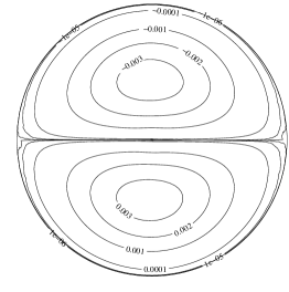
$\leftarrow$ $\leftarrow$

Figure 3: Qualitative behaviour of the streamlines and the axial velocity for Newtonian flows with $\mathcal{R}e\!=\!5$ and $\delta\!=\!0.2$.

For inertial Newtonian fluids (${\cal R}e\!\neq\!0$) a slight curvature of the pipe axis induces centrifugal forces on the fluid and consequently secondary flows, sending fluid outward along the symmetry axis and returning along the upper and lower curved surfaces. A pair of symmetric vortices is then superposed to the Poiseuille flow. This can be seen in Figure 3, where we contours of the axial velocity and the stream-function are presented for ${\cal R}e=5$ and $\delta=0.2$.
The solutions obtained with FEM and Robertson’s perturbation method show a good agreement, in accordance with the predictions. In particular, for this value of the curvature ratio, we can observe a shift from the center. The secondary flow is counter-clockwise in the upper half of the cross–section and clockwise in the lower half.

$\psi_{\max}$ $\psi_{\min}$ $\mathcal{R}\!e$

Figure 4: Profile of the extrema values of the stream function for inertial Newtonian flows.

As already known, the streamlines corresponding to the Newtonian flows show a qualitative and quantitative symmetry relatively to the axis $r=0$. To point out this phenomenon, and for comparison purposes, we first plot the profile of the extrema values of the stream function for different Reynolds numbers. As can be seen in Figure 4, the modulus of the extrema increase with Reynolds numbers.

5.2 Creeping viscoelastic flows

In this section, we are interested in the viscoelastic behaviour of the fluid in the case of creeping flows, and especially in the behaviour of the secondary motions. Our numerical results (using the FEM) indicate changes in the flow characteristics and suggest that at zero Reynolds number, fluid viscoelasticity promotes a secondary flow.

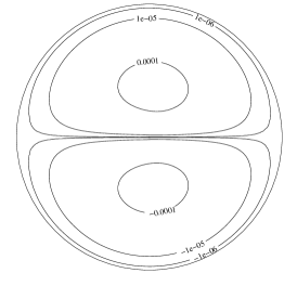
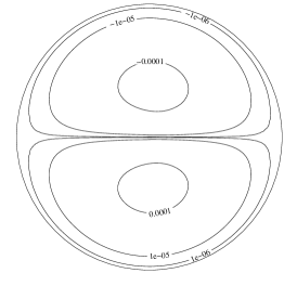
$\rightarrow$ $\rightarrow$	$\leftarrow$ $\leftarrow$
(a)$\ \alpha=-0.01$	(b)$\ \alpha=0.01$

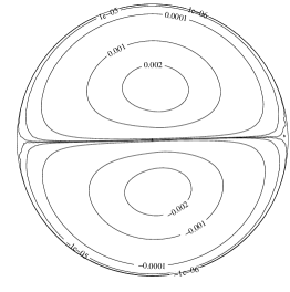
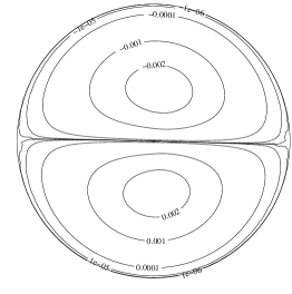
$\rightarrow$ $\rightarrow$	$\leftarrow$ $\leftarrow$
(c)$\ \alpha=-0.2$	(d)$\ \alpha=0.2$

Figure 5: Qualitative behaviour of the streamlines and the axial velocity for creeping viscoleastic flows with $\delta\!=\!0.2$.

In a first step, we consider creeping fluids that are compatible with thermodynamics in the sense that the motions meet the Clausius-Duhem inequality (the viscoelastic parameter $\alpha$ is nonnegative). In Figure $\ref{creeping3}_{b}$ and Figure $\ref{creeping3}_{d}$, the streamlines are plotted for $\alpha=0.01$ and $\alpha=0.2$. As in the Newtonian case, the secondary flows are characterized by two counter-rotating vortices and their magnitude increase with the elastic level (see Figure $\ref{psi_extrema_creep}_{b}$). The only difference is that the flows remain symmetric relatively to an axis which is identical to the pipe centerline for $\alpha$ small and slightly rotates clockwise when $\alpha$ increases (see Figures $\ref{creeping3}_{b}$ and $\ref{creeping3}_{d}$).

$\psi_{\max}$ $\psi_{\min}$ $\alpha$	$\psi_{\max}$ $\psi_{\min}$ $\alpha$
(a)$\ \alpha$ negative	(b) $\ \alpha$ positive

Figure 6: Profile of the extrema values of the stream function for creeping viscoelastic flows.

In a second step, we consider creeping fluids that are not compatible with the thermodynamics ($\alpha$ is negative). As in the positive case, the secondary flows involve non-zero values whose magnitude increase with $|\alpha|$ (see Figure $\ref{psi_extrema_creep}_{a}$). However, their behaviour is not similar. In particular, the orientation of the contours of the stream function is opposite. Moreover, the flow is symmetric relatively to an axis which is identical to the pipe centerline for $|\alpha|$ small, and slightly rotates counter-clockwise when $|\alpha|$ increases (see Figures $\ref{creeping3}_{a}$ and $\ref{creeping3}_{c}$).

5.3 Inertial viscoelastic flows

Now, we are concerned with second-grade fluids where the Reynolds number is non-zero, and with the combined effect of inertia and viscoelasticity.

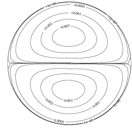
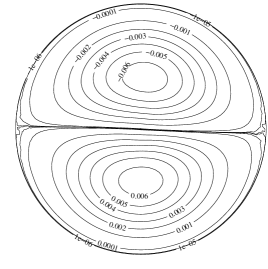
$\leftarrow$ $\leftarrow$	$\leftarrow$ $\leftarrow$
(a)$\ \alpha=0.01$	(b)$\ \alpha=0.3$

Figure 7: Effect of the viscoelasticity on the streamlines with ${\mathcal{R}}e=5$ and $\delta=0.2$.

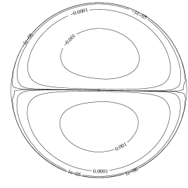
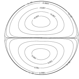
$\leftarrow$ $\leftarrow$	$\leftarrow$ $\leftarrow$
(g) $\mathcal{R}e=1$	(h) $\mathcal{R}e=5$

Figure 8: Effect of the inertia on the streamlines with $\alpha=0.1$ and $\delta=0.2$.

As in the previous section, we first consider the case where the thermodynamics are satisfied. Setting the Reynolds to $5$ and increasing the viscoelastic parameter, we observe that the inertial and creeping viscoelastic flows have the same behaviour: globally Newtonian, with lost of the symmetry relatively to the horizontal axis (see Figure 7). This symmetry is recovered if we fix the viscoelastic parameter and increase the Reynolds number (see Figure 8). Also, the magnitude of the secondary flows increase with $\alpha$ (see Figure $\ref{extrema_viscoinert}_{b}$).

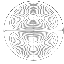
$\leftarrow$ $\leftarrow$
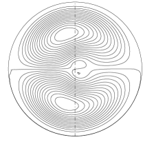
(a) $\ \alpha=-0.01$	(b) $\ \alpha=-0.1$	(c) $\ \alpha=-0.2$
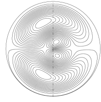
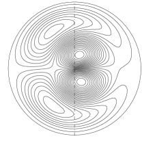
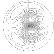
(d) $\ \alpha=-0.25$	(e) $\ \alpha=-0.3$	(f) $\ \alpha=-0.35$
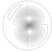
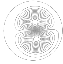
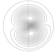
		$\rightarrow$ $\rightarrow$
(g)$\ \alpha=-0.4$	(h)$\ \alpha=-0.45$	(i)$\ \alpha=-0.5$

Figure 9: Effects of the viscoelasticity on the streamlines with ${\mathcal{R}}e=5$ and $\delta=0.2$ with $\alpha$ negative.

The case of negative viscoelastic parameters is more complex. When $\alpha$ is negative and small ($|\alpha|=0.01$), the nature and magnitude of the flow is qualitatively identical to that of a Newtonian fluid, the inertial effect being more pronounced and no effect due to viscoelasticity appears. When $|\alpha|$ increases, the solution obtained by FEM shows reversal flows whose nature is very close to that obtained in the case considered in the previous section when the secondary motion was generated by fluid viscoelasticity.

Figure 9  presents the streamlines for different values of $\alpha$ in the interval $[-0.01;-0.5]$. For $\alpha=-0.01$ we are still in the Newtonian regime. Two counter-rotating vortices appear, and the streamlines in the core region are more dense than elsewhere. However, in Figure $\ref{visco-curve1}_{b}$, a slight modification is already visible with the displacement of the vortices towards the inner wall. As $|\alpha|$ increases, these facts become more pronounced. The values between $\alpha=-0.3$ and $\alpha=-0.2$ seems to be critical. The distortion of the streamlines is even more dramatic, and in addition to the vortices described below, another couple of vortices appear in the core region (see Figure $\ref{visco-curve1}_{c}$). Interestingly, the values in this part of the cross-section have an opposite sign to the ones near the boundaries, suggesting that the core is the transition region and that the reversal from one state to another initiates there. This is confirmed by the results obtained for the cases where $\alpha=-0.3,-0.35,-0.4$, showing that the reversal secondary flows grow around the new couple of vortices and that the changes occur from the core region to the regions near the boundary. It is clear that the size and strength of the new pair of vortices is more important, while a slackening of the streamlines and vortices corresponding to the Newtonian state is observed. In Figure $\ref{visco-curve1}_{g}$ the transition from one regime to the other is completed. Finally, for $\alpha=-0.45$ due to the combined effect of curvature and viscoelasticity, we observe a slight displacement of the center of the vortices to the outer wall. The same modifications can be observed in the quantitative bahaviour of the stream function. In particular, as can be seen in Figure $\ref{extrema_viscoinert}_{a}$, the modulus of the corresponding extremum values decrease for $|\alpha|\in[0,0.25]$, achieves a critical value for $|\alpha|\in[0.25,0.3]$ and increase for $|\alpha|\geq 0.3$.

$\psi_{\max}$ $\psi_{\min}$ $\alpha$	$\psi_{\max}$ $\psi_{\min}$ $\alpha$
(a)$\ \alpha$ negative	(b) $\ \alpha$ positive

Figure 10: Profile of the extrema values of the stream function for inertial viscoelastic flows with ${\cal R}e$=$5$ and $\delta$=$0.2$.

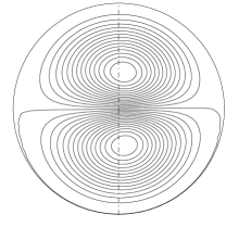
$\rightarrow$ $\rightarrow$
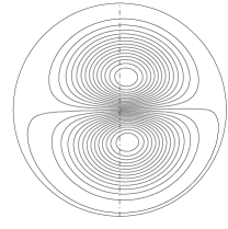
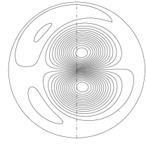
(a) $\mathcal{R}e=0.5$	(b) $\mathcal{R}e=1.0$	(c) $\mathcal{R}e=1.4$
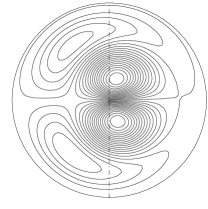
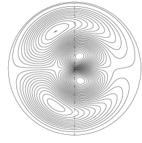
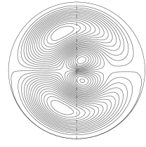
(d) $\mathcal{R}e=1.6$	(e) $\mathcal{R}e=1.8$	(f) $\mathcal{R}e=2.0$
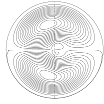
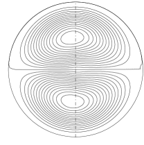
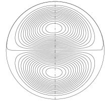
		$\leftarrow$ $\leftarrow$
(g) $\mathcal{R}e=2.5$	(h) $\mathcal{R}e=5.0$	(i) $\mathcal{R}e=10.0$

Figure 11: Effects of the inertia on the streamlines with $\alpha=-0.1$ and $\delta=0.2$.

$\psi_{\max}$ $\psi_{\min}$ $\mathcal{R}\!e$

Figure 12: Profile of the extrema values of the stream function for inertial viscoelastic flows with $\alpha$=$-0.01$ and $\delta$=$0.2$.

Let us now consider the reversal phenomenon. Fixing the parameters $\alpha$, we study the effect of fluid inertia. Setting $\alpha$=$-0.1$ and $\delta$=$0.2$, we present in Figure 11 the contour plots of the stream function for different values of ${\cal R}e$ in the interval $[0.5,4]$. For ${\cal R}e=0.5$, the viscoelasticity is dominant and the inertial forces have no real effect on the secondary flows. For ${\cal R}e=1.4$, some modifications occur. The streamlines in the core region appear to be less dense, the size of the couple of vortices is smaller, the flow is driven near the wall pipe. Moreover, we observe the formation of boundary layer flows, with a pair of weak and elongated vortices. As Reynolds number increases, the boundary layer flows increase rapidly. The vortices in the core region are weaker, while the streamlines near the pipe wall are more dense and distorted, and a strenghthening of the new vortices becomes clear. There is evidence that in contrast with the case where the viscoelasticity dominates, the wall pipe here is the transition region from the viscoelastic state to the inertial one, and that the reversal flows, formed near the boundary around the new vortices, develop and drive the flow to the center of the pipe. Finally, we can conclude that for sufficiently large Reynolds number the secondary flows behave as in the Newtonian case superimposing the $\alpha$ parameter influence.

6 Conclusion

The finite element numerical simulations presented in this work provide relevant information on the qualitative and quantitative behaviour of steady fully developed flows of second-grade fluids in curved pipes of circular cross section and arbitrary curvature ratio, driven by a pressure drop. As stated above, the main feature of curved pipe flows is the existence of secondary motions which are clearly related to small changes with respect to the different parameters of the problem. The numerical tests presented here show that secondary flows are promoted by both viscoelasticity and inertia with a globally newtonian behaviour when the fluids are compatible with the thermodynamics. The more complex case of negative viscoelastic parameters show that the viscoelasticity and the inertia have opposite effects.
Acknowledgements. The second author was supported by Centro de Investigação em Matemática e Aplicações (CIMA) through the grant UID/MAT/04674/2013 of FCT-Fundação para a Ciência e a Tecnologia.

References

- [1] M. Amara, C. Bernardi, V. Girault and F. Hecht, Regularized finite element discretizations of a grade-two fluid model, Int. J. Num. Meth. Fluids 48 (2005) 1375–1414.
- [2] N. Arada, P. Correia and A. Sequeira, Analysis and finite element simulations of a second-order fluid model in a bounded domain, Numerical Methods for Partial Differential Equations, 23 (2007) 1468–1500.
- [3] N. Arada, M. Pires and A. Sequeira, Viscosity effects on flows of generalized Newtonian fluids through curved pipes, Computers and Mathematics with Applications, 53 (2007) 625–646.
- [4] N. Arada, M. Pires and A. Sequeira, Numerical simulations of shear-thinning Oldroyd-B fluids in curved pipes, IASME Transactions, Issue 6, 2 (2005) 948-959.
- [5] S. A. Berger, L. Talbot and L.-S. Yao, Flow in curved pipes, Ann. Rev. Fluid Mech., 15 (1983) 461-512.
- [6] R. B. Bird, R. C. Armstrong and O. Hassager, Dynamics of polymeric liquids, John Wiley & Sons, New York (1987).
- [7] H. A. Barnes and K. Walters, On the flow of viscous and elastico-viscous liquids through straight and curved pipes, Proc. Roy. Soc. Lond., A 314 (1969) 85–109.
- [8] P. J. Bowen, A.R. Davies and K. Walters, On viscoelastic effects in swirling flows, J. Non–Newtonian Fluid Mech. 38 (1991) 113–126.
- [9] P. Correia, Numerical simulations of a non–Newtonian fluid flow model using finite element methods, PhD Thesis, IST, Lisbon, 2004.
- [10] V. Coscia and A. Robertson, Existence and uniqueness of steady, fully developed flows of second order fluids in curved pipes, Math. Models Methods Appl. Sci. 11 (2001) 1055–1071.
- [11] W.R. Dean, Note on the motion of fluid in curved pipe, Philos. Mag. 4 (1927) 208–223.
- [12] W.R. Dean, The streamline motion of fluid in curved pipe, Philos. Mag. 5 (1928) 673–695.
- [13] Y. Fan, R. I. Tanner and N. Phan-Thien, Fully developed viscous and viscoelastic flows in curved pipes, J. Fluid Mech., 440 (2001) 327-357.
- [14] G.P. Galdi and A. Sequeira, Further existence results for classical solutions of the equations of second–grade fluid, Arch. Rational Mech. Anal. 128 (1994) 297–312.
- [15] V. Girault and L. R. Scott, Finite element discretizations of a two-dimensional grade-two fluid model, M2AN 35 (2002) 1007–1053.
- [16] H. Ito, Flow in curved pipes, JSME Int. J., 30 (1987) 543-552.
- [17] W. Jitchote and A.M. Robertson, Flow of second order fluids in curved pipes, J. Non–Newtonian Fluid Mech. 90 (2000) 91–116.
- [18] A. M. Robertson, On viscous flow in curved pipes of non-uniform cross section, Inter. J. Numer. Meth. fluid. 22 (1996) 771–798.
- [19] W.Y. Soh and S.A. Berger, Fully developed flow in a curved pipe of arbitrary curvature ratio, Int. J. Numer. Meth. Fluid. 7 (1987) 733–755.