Refining the scalar and tensor contributions in $\tau\to\pi\pi\pi\nu_{\tau}$ decays

Abstract

In this article we analyze the contribution from intermediate spin–0 and spin–2 resonances to the $\tau\to\nu\pi\pi\pi$ decay by means of a chiral invariant Lagrangian incorporating these mesons. In particular, we study the corresponding axial-vector form-factors. The advantage of this procedure with respect to previous analyses is that it incorporates chiral (and isospin) invariance and, hence, the partial conservation of the axial-vector current. This ensures the recovery of the right low-energy limit, described by chiral perturbation theory, and the transversality of the current in the chiral limit at all energies. Furthermore, the meson form-factors are further improved by requiring appropriate QCD high-energy conditions. We end up with a brief discussion on its implementation in the Tauola Monte Carlo and the prospects for future analyses of Belle’s data.

1 Introduction

The aim of this letter is to provide a coherent description of the impact of scalar ($J^{PC}=0^{++}$) and tensor ($J^{PC}=2^{++}$) mesons in tau decays with three pions in the final state. The four targets of this theoretical analysis are

• Chiral invariance and (partial) axial-vector current conservation: the chiral invariant Lagrangian framework considered in this letter ensures the right QCD symmetries and leads to a hadronic matrix element which is transverse ($\partial_{\mu}J_{A}^{\mu}=0$) in the chiral limit $m_{q}\to 0$ and where longitudinal corrections come naturally suppressed by $m_{q}$. In addition, as isospin is a subgroup of the chiral symmetry, our chiral invariant Lagrangian approach yields the right relation between the $\pi^{0}\pi^{0}\pi^{-}$ and $\pi^{-}\pi^{-}\pi^{+}$ tau decay form-factors, prescribed by isospin symmetry Girlanda:1999fu , without any further requirement. Likewise, we will be always assuming the other symmetries of QCD, parity and charge conjugation. 

• Low-energy limit: the construction of a general chiral invariant Lagrangian that includes the chiral pseudo-Goldstones and the meson resonances ($1^{++}$ axial-vector, $2^{++}$ tensor, etc.) ensures the right low-energy structure and the possibility to match the low-energy effective field theory (EFT) of QCD, Chiral Perturbation Theory ($\chi$PT).

• On-shell description: previous works, in spite of neglecting the previous principles, have performed a fine work in describing the decays through axial-vector and tensor resonances when their intermediate momenta are near their mass shell Castro:2011zd ; CLEO:1999 . Our outcome reproduces these previous results when the momentum $k$ flowing through the intermediate resonance propagator becomes on-shell, this is, when $k^{2}\approx M_{R}^{2}$ (for the corresponding $k$ and $M_{R}$). The chiral invariant Lagrangian ensures that the previous properties are fulfilled also off-shell ($k^{2}\neq M_{R}^{2}$).

• High-energy limit: by imposing high-energy conditions and demanding the behaviour prescribed by QCD for the form-factors at short-distances we will constrain the resonance parameters. Implementing these QCD principles will make our theoretical determination phenomenologically predictive.

This resonance chiral theory (R$\chi$T) approach to the $3\pi$ tau decay was considered in the past taking into account the impact of the vector and axial-vector resonances Dumm:2009va . The corresponding current has been implemented into the Monte Carlo event generator Tauola Shekhovtsova:2012ra . The comparison with the unfolded distributions from the preliminary BaBar Collaboration analysis Nugent:2013ij for the three-prong mode has demonstrated the mismatch in the low-energy part of the two-pion spectrum Shekhovtsova:2012ra and was associated with the lack of the scalar meson multiplet in the original R$\chi$T current Dumm:2009va . The scalar resonance contribution was later added to the three pion current phenomenologically in Ref. Nugent:2013hxa . However, the corresponding part does not obey isospin symmetry Finkemeier:1996 ; Girlanda:1999fu and, as a result, does not reproduce the proper chiral low-energy behaviour (see the discussion in Sec. 2 and App. A).

This letter focuses on the impact of the lowest scalar ($\sigma$ and $f_{0}(980)$) resonances and the isosinglet tensor $f_{2}(1270)$, which may be directly produced from the $W^{-}$ or generated via an intermediate pion or an $a_{1}$ state. Also we discuss the implementation of the associated currents into Tauola and present an estimate of tensor and scalar contributions to the three-pion partial width. In Sec. 2, one finds the general formulae for the three-pion axial-vector form-factor (AFF): the Lorentz structure decomposition and the isospin relation between $\pi^{-}\pi^{-}\pi^{+}$ and $\pi^{0}\pi^{0}\pi^{-}$ channels. In order to avoid any possible double-counting we have separated the contributions to the three-pion AFF in the following way: 1) previous $3\pi$-AFF computations Dumm:2009va ; Shekhovtsova:2012ra incorporate the diagrams including vector resonance exchanges and non-resonant contributions from the ${\cal O}(p^{2})$ $\chi$PT Lagrangian rcht ; 2) Sec. 3 provides the contribution to the $3\pi$-AFF from diagrams with scalar exchanges; 3) the contribution due to spin–2 resonance exchanges is discussed in Sec. 4. Sec. 5 is dedicated to the implementation in the Monte Carlo generator Tauola and some basic numerical results. We provide the conclusions in Sec. 6 and some technical details have been relegated to the Appendices.

2 Axial-vector form-factor into three pions: general formulae

The matrix element of the tau-decay into the three pions is determined in terms of the transverse form-factors $\mathcal{F}_{1}$, $\mathcal{F}_{2}$ and $\mathcal{F}_{3}$ and a longitudinal one $\mathcal{F}_{P}$:

$$\langle\,3\pi|\bar{d}\gamma^{\mu}\gamma_{5}u|0\,\rangle = H^{3\pi}(q^{2},s_{1},s_{2})^{\mu}$$ (1)

$$= i\,P_{T}^{\mu\nu}(q)\bigg{[}\mathcal{F}_{1}(s_{1},s_{2},q^{2})\,\,(p_{1}-p_{3})_{\nu}\,\,+\,\,\mathcal{F}_{2}(s_{1},s_{2},q^{2})\,\,(p_{2}-p_{3})_{\mu}$$

$$+\,\,\mathcal{F}_{3}(s_{1},s_{2},q^{2})\,\,(p_{1}-p_{2})_{\mu}\bigg{]}\,\,+\,\,i\,q_{\mu}\,\,\mathcal{F}_{P}(s_{1},s_{2},q^{2})\,,$$

with $q=p_{1}+p_{2}+p_{3}$, $s_{1}=(p_{2}+p_{3})^{2}$, $s_{2}=(p_{3}+p_{1})^{2}$ and $s_{3}=(p_{1}+p_{2})^{2}$, and $P_{T}(q)^{\mu\nu}=g^{\mu\nu}-q^{\mu}q^{\nu}/q^{2}$. The three transverse form-factors are linearly dependent and we will leave only $\mathcal{F}_{1}$ and $\mathcal{F}_{2}$ as our basis. The longitudinal form-factor $\mathcal{F}_{P}$ vanishes in the chiral limit and is suppressed by $m_{\pi}^{2}/q^{2}$ Dumm:2009va . Our formulae for the hadronic form-factors will be calculated in the isospin limit. We will take $m_{\pi}=(m_{\pi^{0}}+2m_{\pi^{+}})/3$ and, in general, apply the relation $q^{2}=s_{1}+s_{2}+s_{3}-3m_{\pi}^{2}$ to express the form-factors in terms of the three independent kinematic variables $q^{2},s_{1},s_{2}$.

Bose symmetry implies that

$$\mathcal{F}_{1}(s_{1},s_{2},q^{2}) = \mathcal{F}_{2}(s_{2},s_{1},q^{2})\,,$$

$$\mathcal{F}_{P}(s_{1},s_{2},q^{2}) = \,\mathcal{F}_{P}(s_{2},s_{1},q^{2})\,,$$ (2)

and therefore there are only two independent form-factors, e.g., $\mathcal{F}_{1}$ and $\mathcal{F}_{P}$.

Isospin symmetry relates the matrix elements with $\pi^{-}\pi^{-}\pi^{+}$ and $\pi^{0}\pi^{0}\pi^{-}$ final states Girlanda:1999fu : 

$$H_{\mu}^{--+}(p_{1},p_{2},p_{3}) = H_{\mu}^{00-}(p_{3},p_{2},p_{1})+H_{\mu}^{00-}(p_{3},p_{1},p_{2})\,.$$ (3)

Thus, the form-factors for $\pi^{-}\pi^{-}\pi^{+}$ and $\pi^{0}\pi^{0}\pi^{-}$ are related in the form

$$\mathcal{F}_{1}^{\pi^{-}\pi^{-}\pi^{+}}(s_{1},s_{2},q^{2}) = \mathcal{F}_{1}^{\pi^{0}\pi^{0}\pi^{-}}(s_{1},s_{3},q^{2})-\mathcal{F}_{1}^{\pi^{0}\pi^{0}\pi^{-}}(s_{2},s_{3},q^{2})-\mathcal{F}_{1}^{\pi^{0}\pi^{0}\pi^{-}}(s_{3},s_{2},q^{2})\,,$$ (4)

$$\mathcal{F}_{P}^{\pi^{-}\pi^{-}\pi^{+}}(s_{1},s_{2},q^{2}) = \mathcal{F}_{P}^{\pi^{0}\pi^{0}\pi^{-}}(s_{1},s_{3},q^{2})+\mathcal{F}_{P}^{\pi^{0}\pi^{0}\pi^{-}}(s_{2},s_{3},q^{2})\,.$$ (5)

It is also possible to revert this expressions and to express the $\pi^{0}\pi^{0}\pi^{-}$ matrix element in terms of the $\pi^{-}\pi^{-}\pi^{+}$ (App. D) but for sake of simplicity, from now on, we will always refer to the $\pi^{0}\pi^{0}\pi^{-}$ form-factors and assume Eqs. (4) and (5) whenever the $\pi^{-}\pi^{-}\pi^{+}$ one is needed. The advantage of our chiral Lagrangian approach is that it implements by default this isospin relation (and Bose symmetry, of course), as isospin is a subgroup of the chiral group.

It is worth to stress that the $\pi^{-}\pi^{-}\pi^{+}$ and $\pi^{0}\pi^{0}\pi^{-}$ hadronic currents are in general not the same Finkemeier:1996 ; Pais:1960zz ; CLEO-isospin . The diagrams with intermediate vector and axial-vector resonances give the same $\mathcal{F}_{1}(s_{1},s_{2},q^{2})$ form-factor up to a global sign difference Dumm:2009va . However, on the contrary to the approach therein, tensor and scalar resonances generate contributions to the $\pi^{-}\pi^{-}\pi^{+}$ and $\pi^{0}\pi^{0}\pi^{-}$ hadronic currents with a different kinematical structure (determined by Eqs. (4) and (5)). For further details on the isospin relation between channels see Refs. Girlanda:1999fu ; Finkemeier:1996 ; Pais:1960zz and App. D. In the next Sections we will focus on the three-pion tree-level production via intermediate scalar and tensor resonances, which will be dressed with appropriate widths when compared to data. Apart from this, we will not incorporate other one-loop contributions like, e.g, the non-resonant triangular topologies with three internal propagators (with the mesons $KKK^{*}$, $\pi\pi\rho$, etc.) and the external pions and $W$ connected at the vertices.

3 The decay $\tau\to\pi\pi\pi\nu_{\tau}$ through scalar resonances

We first consider the three-pion production via an intermediate state with a scalar $S$ and a pion. If isospin and C-parity are conserved then G-parity requires that the scalar resonance has isospin fulfilling $(-1)^{I}=+1$ –i.e., even isospin–, which in our case implies $I=0$.

The hadronic matrix element for the transition from an axial-vector current into an isosinglet scalar $S$ and a pion has the general Lorentz structure rcht-FFs

$$\langle\,S_{I=0}(k)\pi^{-}(p)|\bar{d}\gamma^{\alpha}\gamma_{5}u|0\,\rangle = -2iP_{T}(q)^{\alpha\nu}\,p_{\nu}\,\mathcal{F}^{a}_{S\pi}(q^{2};k^{2})\,\,+\,\,i\,q^{\alpha}\,\mathcal{H}^{a}_{S\pi}(q^{2};k^{2})\,,$$ (6)

where $q=k+p$ and the scalar function $\mathcal{F}^{a}_{S\pi}(q^{2})$ provides AFF into $S\pi$ in the chiral limit, as $\mathcal{H}^{a}_{S\pi}$ is suppressed by $m_{\pi}^{2}$ due to the partial conservation of the axial-vector current. Here the isosinglet scalar $S_{I=0}$ refers to the resonance without $s\bar{s}$ component, $S_{I=0}\sim u\bar{u}+d\bar{d}$, which we will relate with the lightest scalar isoscalar resonance, the $f_{0}(500)$ or $\sigma$. We leave the discussion of the properness of this approach for a next Section: here we will just assume the large-$N_{C}$ framework tHooft:1973alw ; tHooft:1974pnl ; Witten:1979kh and the phenomenological implementation will be later worked out.

In Fig. 1, we show the three relevant diagrams that must be taken into account in the $S\pi$ production at large $N_{C}$ (and analogously later in the production of a tensor resonance $T$ and a pion): a) the direct production $W^{-}\to S\pi^{-}$; b) the intermediate $\pi^{-}$ production $W^{-}\to\pi^{-}\to S\pi^{-}$; c) and the scalar production through an intermediate axial-vector resonance, $W^{-}\to a_{1}\to S\pi^{-}$.

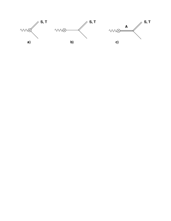
Figure 1: Relevant diagrams for the hadronic tau decays into an isosinglet scalar $S$ and a pion and its corresponding AFF (similar to those for the decay into a isosinglet tensor $T$ and a pion). Single straight lines stand for pions and the wavy line for the external axial-vector source (from an incoming $W^{-}$).

3.1 The R$\chi$T Lagrangian for scalar fields

The resonance Lagrangian has the generic structure

$$\mathcal{L}_{\rm R\chi T} = \mathcal{L}_{\rm non-R}\,+\,\sum_{R}\mathcal{L}_{R}\,+\,\sum_{R,R^{\prime}}\mathcal{L}_{R\,R^{\prime}}\,+\,...$$ (7)

which respectively contains operators without resonances, operators with one resonance field, terms with two resonance fields, etc. In the case of the tau decay into three pions through an intermediate scalar production, the relevant chiral invariant Lagrangian consists of three parts:

• Operators with one resonance field rcht :

  $$\mathcal{L}_{A} = \frac{\displaystyle F_{A}}{\displaystyle 2\sqrt{2}}\langle\,A_{\mu\nu}f_{-}^{\mu\nu}\,\rangle\,,$$

  $$\mathcal{L}_{S} = c_{d}\langle\,Su_{\mu}u^{\mu}\,\rangle+c_{m}\langle\,S\chi_{+}\,\rangle\,,$$ (8)

• Operators with an axial-vector and a scalar field (which provides the $AS\pi$ vertex in diagram c) in Fig. 1) rcht-FFs :

  $$\mathcal{L}_{AS} = \lambda_{1}^{AS}\langle\,\{\nabla_{\mu}S,A^{\mu\nu}\}u_{\nu}\,\rangle\,.$$ (9)

  Operators of the $\mathcal{L}_{AS}$ Lagrangian that do not contribute to the $AS\pi$ vertex are not shown here rcht-FFs .

• Operators without resonance fields Gasser:1983yg ; Gasser:1984gg ; rcht :

  $$\mathcal{L}^{(2)}_{\rm non-R} = \frac{\displaystyle F^{2}}{\displaystyle 4}\langle\,u_{\mu}u^{\mu}+\chi_{+}\,\rangle\,,$$ (10)

  This non-resonant $O(p^{2})$ Lagrangian generates the $W^{-}\to\pi^{-}$ transition vertex in Fig. 1.b. It also provides an $O(p^{2})$ contribution without intermediate resonances to the $\pi\pi\pi$ AFF which was accounted in previous analyses Dumm:2009va . Thus, in order to avoid double counting, we will not consider these non-resonant $\pi\pi\pi$ AFF diagrams.

For the axial-vector field $A_{\mu\nu}=A_{\mu\nu}^{a}\lambda^{a}/\sqrt{2}$ we have used the antisymmetric tensor representation rcht ; op6rxt , with

$$A_{\mu\nu} = \left(\begin{array}[]{ccc}0&a_{1}^{+}&0\\ a_{1}^{-}&0&0\\ 0&0&0\end{array}\right)_{\mu\nu}\,\,\,+\,\,\,...$$ (14)

with the dots standing for the other axial-vector resonances of the multiplet, which will not be relevant in the present study. For the chiral tensors containing the light pseudoscalars, the masses and the external vector and axial-vector source fields we used chpt ; rcht

$$U=u^{2}=\exp\{\pi^{a}\lambda^{a}/F\}\,,\qquad D_{\mu}U=\partial_{\mu}U-ir_{\mu}U+iU\ell_{\mu}\,,\qquad u_{\mu}=iu^{\dagger}(D_{\mu}U)u^{\dagger}\,,$$

$$\chi_{\pm}=u^{\dagger}\chi u^{\dagger}\pm u\chi^{\dagger}u\,,\qquad f_{\pm}^{\mu\nu}=uF_{L}^{\mu\nu}u^{\dagger}\pm u^{\dagger}F_{R}^{\mu\nu}u\,,\qquad\nabla_{\mu}\cdot=\partial_{\mu}\cdot+[\Gamma_{\mu},\cdot]\,,$$

$$\Gamma_{\mu}=\frac{\displaystyle 1}{\displaystyle 2}\left\{u^{\dagger}(\partial_{\mu}-ir_{\mu})u+u(\partial_{\mu}-i\ell_{\mu})u^{\dagger}\right\}\,,$$ (15)

with the scalar-pseudoscalar source $\chi=2B_{0}$diag$(m_{u},m_{d},m_{s})+...$ (the dots stand for terms not relevant for this calculation) and $F_{L}^{\mu\nu}$ and $F_{R}^{\mu\nu}$ the field strength tensors of the left and right sources, respectively $\ell_{\alpha}$ and $r_{\alpha}$. If we are only interested in the $W^{\pm}$ currents one takes $\ell_{\alpha}=\frac{g}{\sqrt{2}}(W_{\alpha}^{+}T_{+}+{\rm h.c.})$ and $r_{\alpha}=0$, with $T_{+}=V_{ud}(\lambda^{1}+i\lambda^{2})/2+V_{us}(\lambda^{4}+i\lambda^{5})/2$. The $\pi^{a}$ generically refer to the $SU(3)$ chiral pseudo-Goldstones ($a=1...8$). At large $N_{C}$ (and for the non-strange current) this process only occurs for the isosinglet scalar $S_{I=0}\sim u\bar{u}+d\bar{d}$, with no $s\bar{s}$ strange quark component:

$$S = \left(\begin{array}[]{ccc}\frac{\displaystyle S_{I=0}}{\displaystyle\sqrt{2}}&0&0\\ 0&\frac{\displaystyle S_{I=0}}{\displaystyle\sqrt{2}}&0\\ 0&0&0\end{array}\right)\,\,\,+\,\,\,...$$ (19)

where the dots stand for other resonances in the multiplet not relevant for the present work.

3.2 AFF into $S\pi^{-}$

Our chiral invariant Lagrangian leads to the AFF prediction, 

$$\mathcal{F}^{a}_{S\pi}(q^{2};k^{2}) = \frac{\displaystyle 2c_{d}}{\displaystyle F_{\pi}}\quad+\quad\frac{\displaystyle\sqrt{2}F_{A}\lambda_{1}^{AS}}{\displaystyle F_{\pi}}\frac{\displaystyle q^{2}}{\displaystyle M_{A}^{2}-q^{2}}\,,$$ (20)

$$\mathcal{H}^{a}_{S\pi}(q^{2};k^{2}) = \frac{\displaystyle 4}{\displaystyle F_{\pi}}\,\frac{\displaystyle m_{\pi}^{2}}{\displaystyle q^{2}(q^{2}-m_{\pi}^{2})}\,\left[c_{d}(qp)+c_{m}q^{2}\right]\,,$$ (21)

with $(qp)=(q^{2}+m_{\pi}^{2}-k^{2})/2$, being $k^{2}=M_{S}^{2}$ for an on-shell scalar (later, when this scalar is considered off-shell and decaying in two pions with momenta $p_{i}$ and $p_{j}$ it will take the value $k^{2}=(p_{i}+p_{j})^{2}$). The $c_{m}$ operator contributes through the $s$-channel pion exchange to the longitudinal form-factor in Eq. (21). 

3.3 $3\pi$-AFF through an intermediate scalar resonance

Considering not only the $S\pi$ production but also the subsequent decay $S\to\pi\pi$ one obtains the corresponding contribution to the $\pi\pi\pi$-AFF.

Using the Lagrangian in Eqs. (9)–(10), we obtain the contribution from scalar resonance exchanges to the $\pi^{0}\pi^{0}\pi^{-}$ AFFs defined in (1),

$$\mathcal{F}_{1}^{\pi^{0}\pi^{0}\pi^{-}}(s_{1},s_{2},q^{2})\bigg{|}_{S} = \frac{\displaystyle 2}{\displaystyle 3}\mathcal{F}_{S\pi}^{a}(q^{2};s_{3})\,\mathcal{G}_{S\pi\pi}(s_{3})\,,$$ (22)

$$\mathcal{F}_{P}^{\pi^{0}\pi^{0}\pi^{-}}(s_{1},s_{2},q^{2})\bigg{|}_{S} = \mathcal{H}^{a}_{S\pi}(q^{2};s_{3})\,\mathcal{G}_{S\pi\pi}(s_{3})\,,$$ (23)

with $qp_{j}=(m_{\pi}^{2}+q^{2}-s_{j})/2$. The $AS\pi$ form-factor is the previous one in Eq. (20) whereas propagation of the isosinglet $S$ and its decay into $\pi\pi$ gives

$$\mathcal{G}_{S\pi\pi}(s_{3}) = \frac{\displaystyle\sqrt{2}}{\displaystyle F_{\pi}^{2}}\,\frac{\displaystyle 1}{\displaystyle M_{S}^{2}-s_{3}}\,[c_{d}(s_{3}-2m_{\pi}^{2})+2c_{m}m_{\pi}^{2}]\,.$$ (24)

Notice that we are giving the full result, including pion mass corrections produced by our Lagrangian in Eqs. (9)–(10).

Requiring that the contribution to the transverse component of the $\Pi_{AA}^{\mu\nu}(q)$ spectral function vanishes implies that $\mathcal{F}^{a}_{S\pi}(q^{2})\longrightarrow 0$ for $q^{2}\to\infty$ (see App. B), giving the constraint rcht-FFs

$$F_{A}\lambda_{1}^{AS} = \sqrt{2}c_{d}\,,$$ (25)

and the form-factor prediction

$$\mathcal{F}^{a}_{S\pi}(q^{2};s_{3}) = \frac{\displaystyle 2c_{d}}{\displaystyle F_{\pi}}\frac{\displaystyle M_{A}^{2}}{\displaystyle M_{A}^{2}-q^{2}}\,.$$ (26)

This high-energy constraint is similar to the asymptotic form-factor high-energy behaviour prescribed by Brodsky-Lepage quark-counting rules Brodsky:1973kr , which imply, for instance, that the pion vector form-factor vanishes like $\sim 1/q^{2}$ at infinite momentum transfer rcht ; Brodsky:1973kr .

The subsequent decay of the scalar into $\pi\pi$ is given by $\mathcal{G}_{S\pi\pi}(s_{3})$ and would provide the absorptive $\pi\pi\pi$ contribution to Im$\Pi_{AA}^{\mu\nu}$. However, in the narrow-width limit for $S$, the three-pion phase-space integral yields a delta function $\delta(s_{3}-M_{S}^{2})$ that sets the $s_{3}$ value to $M_{S}^{2}$. Thus, the integral is factorized into the two-body integration of $|\mathcal{F}^{a}_{S\pi}(q^{2})|^{2}$ over the $S\pi^{-}$ phase-space and a constant angular integration over the phase-space of the two pions produced by the scalar. Therefore, in this limit, the large $q^{2}$ behaviour of this three-pion contribution to the spectral function is ruled by the form-factor $\mathcal{F}^{a}_{S\pi}(q^{2})$ in the way dictated by Eq. (83) (up to a global constant factor). We will use this theoretical large–$N_{C}$ information and use it to constrain our form-factor even if we will later model it in order to include important subleading effects in $1/N_{C}$ such as the $\sigma$ width.

The $S\pi$ AFF is then ruled by the $c_{d}$ coupling in the limit $m_{\pi}^{2}\ll q^{2}$. Even though its precise experimental value is still unclear, most analyses agree on a value $c_{d}\sim 30$ MeV (see Escribano:2010wt and references therein). For a discussion on its numerical impact on the spectral distributions, see Sec. 5.

3.4 Scalar resonance widths

The lightest isoscalar particle is the broad scalar $\sigma$, with $M_{\sigma}^{\rm pole}=441^{+16}_{-\,8}$ MeV, $\Gamma_{\sigma}^{\rm pole}=544^{+18}_{-25}$ MeV CCL-sigma . It is thought to contain mostly just $u$ and $d$ quark components, where the two–pion channel is its only kinematically allowed decay. On the other hand, as it follows from its predominant decay into $K\bar{K}$, the next scalar isosinglet, the $f_{0}(980)$, is considered to have a large strange quark component, being its $n\pi$ decay modes are suppressed. However, for sake of completeness we will include both isoscalars into consideration.

A first approach to the physical QCD case is provided by the inclusion of a $\sigma$–$f_{0}(980)$ splitting through the substitution Escribano:2006mb ; Escribano:2010wt ,

$$\frac{\displaystyle 1}{\displaystyle M_{S}^{2}\,-\,s}\qquad\longrightarrow\qquad\frac{\displaystyle\cos^{2}\phi_{S}}{\displaystyle M_{\sigma}^{2}\,-\,s}\,\,+\,\,\frac{\displaystyle\sin^{2}\phi_{S}}{\displaystyle M_{f_{0}}^{2}\,-\,s}\,,$$ (27)

where $\phi_{S}$ is the scalar mixing angle. For the $\sigma-f_{0}$ mixing we will use the numerical value $\phi_{S}=-8^{\circ}$ Escribano:2006mb .

Due to the $\sin^{2}\phi_{S}$ suppression the $f_{0}(980)$ produces a clearly subdominant effect with respect to the impact of the broad $\sigma$. However, the comparison of the modified R$\chi$T spectra Nugent:2013hxa   with the unfolded distributions Nugent:2013ij from the preliminary BaBar Collaboration $\tau\to\nu_{\tau}\pi\pi\pi$ analysis has shown a statistically significant mismatch: the $\pi^{+}\pi^{-}$ experimental spectral function is well reproduced up to 1 GeV except for a small sharp bump concentrated at 980 MeV which differs from the $f_{0}$-absent theoretical R$\chi$T expression by a few percent. The inclusion of the $f_{0}$ and its occurrence here via the $\sigma-f_{0}$ mixing in Eq. (27) is expected to improve the phenomenological description of the data.

3.4.1 Incorporating the $\sigma$ meson width

So far in previous Sections we have carried on a large-$N_{C}$ computation where one had an intermediate exchange of narrow-width scalars. This approximation seems to be suitable for the $f_{0}(980)$. However, the $\sigma$ meson is a broad resonance and the effect of its width is non-negligible. It is not our intention to enter here in the discussion of the $\sigma$ nature but, rather, to propose an improved parametrization of its effect on the $\tau\to\nu\pi\pi\pi$ decay that incorporates the features described in the introduction. For this, we follow the successful analysis of subleading $1/N_{C}$ effects in scalar exchanges in the $\eta^{\prime}\to\eta\pi\pi$ process Escribano:2010wt : after considering the scalar splitting in (27), we incorporate the “dressed” $\sigma$ propagator in a similar way by performing the substitution

$$\frac{\displaystyle 1}{\displaystyle M_{\sigma}^{2}\,-\,s}\qquad\longrightarrow\qquad\frac{\displaystyle 1}{\displaystyle M_{\sigma}^{2}\,-\,s\,-\,f_{\sigma}(s)\,-\,iM_{\sigma}\Gamma_{\sigma}(s)}\,,$$ (28)

with

$$f(s) = c_{\sigma}s^{k}\,{\rm Re}\overline{B}_{0}(s,m_{\pi}^{2},m_{\pi}^{2})\,=\,\frac{\displaystyle c_{\sigma}\,s^{k}}{\displaystyle 16\pi^{2}}\left[2-\rho_{\pi}(s)\ln{\frac{\rho_{\pi}(s)+1}{1-\rho_{\pi}(s)}}\right]\,,$$

$$M_{\sigma}\Gamma_{\sigma}(s) = c_{\sigma}s^{k}\,{\rm Im}\overline{B}_{0}(s,m_{\pi}^{2},m_{\pi}^{2})\,=\,\frac{\displaystyle c_{\sigma}\,\rho_{P}(s)\,s^{k}}{\displaystyle 16\pi}\,,$$ (29)

in the fashion of Gounaris and Sakurai GS-rho and the Chew and Mandelstam dispersive integral Chew:1960iv . We will use the parameters $M_{\sigma}$ and $c_{\sigma}$ tuned such that one recovers the right position for the $\sigma$ pole, $M_{\sigma}^{\rm pole}=441^{+16}_{-\,8}$ MeV, ${\Gamma_{\sigma}^{\rm pole}=544^{+18}_{-25}}$ MeV CCL-sigma . The function,

$$\overline{B}_{0}(s,m_{P}^{2},m_{P}^{2}) = \frac{1}{16\pi^{2}}\left[2-\rho_{P}(s)\ln{\frac{\rho_{P}(s)+1}{\rho_{P}(s)-1}}\right]$$ (30)

$$=\frac{1}{16\pi^{2}}\left[2-\rho_{P}(s)\ln{\frac{\rho_{P}(s)+1}{1-\rho_{P}(s)}}\,+\,i\pi\rho_{P}(s)\right]\,,$$

is    the    subtracted    two–point    Feynman    integral    ($\overline{B}_{0}(0,m_{P}^{2},m_{P}^{2})=0$),    with ${\rho_{P}(s)\equiv\lambda(s,m_{P}^{2},m_{P}^{2})^{\frac{1}{2}}/q^{2}=\sqrt{1-4m_{P}^{2}/s}}$.

One of the crucial points of the parametrization Escribano:2010wt employed here is that it incorporates the real part of the logarithm that comes along with the imaginary part $-iM_{\sigma}\Gamma_{\sigma}(s)$ on the basis of analyticity. In the case of narrow-width resonances, these real logs are essentially negligible and can be dropped. However, if their corresponding imaginary part is large one naturally expect the appearance of equally large real logarithms. Moreover, any attempt to match NLO $\chi$PT at low-energies must incorporate both the real and imaginary parts of the logs. Even though our simple approach Escribano:2010wt can be further refined, it already contains some of the basic ingredients that makes this matching possible. Other works that incorporate the real and imaginary parts of the logarithm in other observables can be found in Refs. ND ; Sdecays .

The power behaviour $k=0$ produces an unphysical bound state in the first Riemann sheet very close below the $\pi\pi$ threshold, which unnaturally enhanced the amplitude in the $\eta^{\prime}\to\eta\pi\pi$ Escribano:2010wt , leading in that work to a very small $S\pi\pi$ coupling $c_{d}=9.9$ MeV. This case seems to be clearly disfavoured from the phenomenological point of view and was discarded in the analysis of Ref. Escribano:2010wt . For $k=1$, the amplitude produces just one pole and its correct position $\sqrt{s^{\sigma}_{\rm pole}}=[(441^{+16}_{-\,8})\,-\,i(544^{+18}_{-25})/2]$ MeV CCL-sigma is recovered for the parameter values $M_{\sigma}=806.4$ MeV and $c_{\sigma}=76.12$.  Power behaviours with $k\geq 2$ are unable to generate the $\sigma$ pole at the right position. For its closest position, the pole mass is slightly larger and the pole width is roughly 100 MeV smaller. Likewise, some spurious poles are produced far from the physical energy range of the problem under study.

For the numerical inputs we will take the $s^{k}$ scaling with $k=1$ in Eq. (29) and the values $M_{\sigma}=806.4$ MeV and $c_{\sigma}=76.12$. In these expressions the constants $M_{\sigma}$ and $c_{\sigma}$ that appear in the denominator are parameters set to agree with the central value of the $\sigma$ pole position $s_{\sigma}^{\rm pole}=(M_{\sigma}^{\rm pole}-i\Gamma_{\sigma}^{\rm pole}/2)^{2}$ from Ref. CCL-sigma .

Our estimate of the rescattering of the $\pi\pi$ system related to the isosinglet scalar is obviously model dependent, as we have introduced an ad hoc splitting and self-energy for the scalar multiplet. The splitting can be easily introduced through the corresponding terms in the Lagrangian, studied in Ref. mass-split . On the other hand, while the $1/N_{C}$ counting would strictly lead to zero-width resonances, finite widths are needed to regularize the $\tau$ decay phase space integrals and compare to data. Hence, they need to be taken into account and analyticity requires the presence of the real logarithm counterparts in the self-energy. However, if these provide a large contribution, it seems that $1/N_{C}$ corrections provide a significant effect in contradiction with the hypothesis of neglecting, e.g., resonance-mediated loops. There is no clear and definitive answer to this issue yet and one of goals of this work is to explore the raised problem. In this article, we assume that this is the only subleading contribution in $1/N_{C}$ which is numerically relevant for the current precision of the analysis. As noticed in Refs. RChT-width ; RGE , the resummation of subleading $1/N_{C}$ corrections can be well defined in perturbation theory and become crucial even for the $\rho(770)$. Following previous scalar resonance studies in this line Escribano:2010wt , we consider this resummation of the one-loop $\pi\pi$ self-energy is also justified, even for the broad $\sigma$: higher order effects absent in the resummation (multimeson channels) are completely negligible below 1 GeV and the one-loop amplitude seems to provide the crucial information in our physical range. Notwithstanding, this $\pi\pi$ final state interaction must be appropriately resummed in the neighbourhood of the resonance pole, as noted in Refs. RChT-width ; RGE . Alternatively one might incorporate the $s$–wave rescattering via unitarization procedures Escribano:2010wt ; ND and related dispersion relations (see, e.g., the semileptonic $B$ decay analysis Kang:2013jaa ). It is important to point out, however, that even in this robust method only the $\pi\pi$ absorptive corrections are incorporated in the analysis (and the most relevant inelastic intermediate channels in some cases).

3.4.2 Incorporating the $f_{0}$ meson width

One can take also into account the $f_{0}(980)$ width in a similar way. Due the $\sin^{2}\phi_{S}$ suppression in (27), the $f_{0}(980)$ produces a clearly subdominant effect with respect to the impact of the broad $\sigma$. The important piece of the self-energy is its imaginary part, being the real part of its corresponding logarithm almost negligible in comparison with the leading contribution $M_{S}^{2}-s$. In the case of the narrow $f_{0}$ resonance, the location of its pole near the $K\overline{K}$ threshold will modify the $f_{0}$ propagator into the well-known Flatté form Flatte:1976xu

$$\frac{\displaystyle 1}{\displaystyle M_{f_{0}}^{2}\,-\,s}\quad\longrightarrow\qquad\frac{\displaystyle 1}{\displaystyle M_{f_{0}}^{2}\,-\,s\,-\,iM_{f_{0}}\Gamma_{f_{0}}(s)}\,,$$ (31)

with

$$M_{f_{0}}\Gamma_{f_{0}}(s) = \frac{\displaystyle c_{f_{0}}M_{f_{0}}^{2}\rho_{K}(s)}{\displaystyle 16\pi}\,,$$ (32)

which is indeed the near threshold expression of the self-energy at lowest order in the non-relativistic expansion in powers of the kaon three-momentum $|\vec{p}_{K}|\sim\rho_{K}(s)$ Braaten:2007dw ; Meng:2014ota . As the self-energy is only relevant for $s\approx M_{f_{0}}^{2}$, one does not need to consider different $c_{f_{0}}s^{k}$ scalings for the loop corrections as we did for the $\sigma$ meson and the different values of $k$ amount just for differences at higher order in the non-relativistic expansion in $\rho_{K}(s)$. For $s_{f_{0}}^{\rm pole}=(M_{f_{0}}^{\rm pole}-i\Gamma_{f_{0}}^{\rm pole}/2)^{2}=(990-i70/2)^{2}$ MeV² pdg   this implies the parameters $M_{f_{0}}=1024$ MeV and $c_{f_{0}}=17.7$. The best estimate, based on Roy equations, gives the value $\sqrt{s_{f_{0}}^{\rm pole}}=(996^{\,+4}_{-14})-i(24^{+11}_{\,-3})$ MeV Moussallam:2011zg . This deviates by less than 1% from the PDG central value we will use in Sec. 5. We do not expect any difference for our numerical result. Likewise, in spite of the fact that we have used the average kaon mass $m_{K}=496$ MeV, the latter result is not very sensitive to the precise position of the $K\overline{K}$ threshold, with $M_{f_{0}}$ and $c_{f_{0}}$ changing by $\pm 0.5\%$ and $\pm 7\%$, respectively, when $m_{K}$ is varied between the charged and neutral kaon mass values. By far the largest effect would be the uncertainty in the $f_{0}$ mass and width with errors of $\pm 20$ MeV and $\pm 30$ MeV, respectively pdg .

Therefore, for the numerical inputs we will take $M_{f_{0}}=1024$ MeV and $c_{f_{0}}=17.7$. 

4 The decay $\tau\to\pi\pi\pi\nu_{\tau}$ through tensor resonances

In this section we focus on tau decay into three pions through an intermediate tensor resonance ($J^{PC}=2^{++}$) in the cascade decay $\tau\,\to\,\nu_{\tau}\,\pi^{-}\,T(\to\pi\pi)$. Our study reproduces the prediction for the tau decay into a tensor resonance and a chiral pseudo-Goldstone Castro:2011zd and expands then for the case of the off-shell tensor resonance.

$G$-parity conservation implies that for the non-strange axial-vector current (with $G=-1$) the tensor resonance produced in combination with a pion must have $G=(-1)^{I}=+1$ and, hence, even isospin. As a consequence of this, it must be an isosinglet in the case of $q\bar{q}$ multiplets ($T=f_{2}(1270)$, $f_{2}(1430)$, $f_{2}^{\prime}(1525),\,f_{2}(1565)...$). In this article we study the impact of the lightest tensor, $f_{2}(1270)$, which dominantly decays into $\pi\pi$ pdg . The $f_{2}^{\prime}(1525)$ mainly goes into $K\overline{K}$ and has a negligible decay into $\pi\pi$ pdg . Our analysis is then restricted to the lowest tensor resonances. We discarded not so well established resonances such as the $f_{2}(1430)$ and $f_{2}(1565)$, whose $\pi\pi$ partial width are not determined in any of the references quoted by PDG pdg . In addition, we would like to stress that, the contribution from the $f_{2}(1270)$ is found to be highly suppressed in our later numerical analysis, as it is placed near the $\pi^{0}\pi^{0}$ spectrum end point (or the $\pi^{+}\pi^{-}$ spectrum for $\tau\to\nu_{\tau}\pi^{-}\pi^{-}\pi^{+}$), $M_{\pi\pi}^{\rm end}=M_{\tau}-m_{\pi^{\pm}}\simeq 1637$ MeV. Thus, heavier $f_{2}$ resonances should have even stronger phase-space suppressions. In particular the $f_{2}(1640)$ and further tensors lie beyond $M_{\pi\pi}^{\rm end}$.

4.1 The R$\chi$T Lagrangian for tensor fields

The relevant part of the chiral invariant Lagrangian for the pion-tensor production (Fig 1) consists in this case of

• Operators with one resonance field rcht ; Zauner:2007 , 

  $$\mathcal{L}_{A} = \frac{\displaystyle F_{A}}{\displaystyle 2\sqrt{2}}\langle\,A_{\mu\nu}f_{-}^{\mu\nu}\,\rangle\,,$$

  $$\mathcal{L}_{T} = g_{T}\langle\,T_{\mu\nu}\{u^{\mu},u^{\nu}\}\,\rangle\,.$$ (33)

• Operators with an axial-vector and a tensor field (which provides the $AT\pi$ vertex in diagram c) in Fig. 1),

  $$\mathcal{L}_{AT\pi} = \lambda_{1}^{AT}\,\langle\,\{T_{\mu\nu},A^{\nu\alpha}\}h_{\alpha}^{\mu}\,\rangle+\lambda_{2}^{AT}\langle\,\{A_{\alpha\beta},\nabla^{\alpha}T^{\mu\beta}\}u_{\mu}\,\rangle\,,$$ (34)

  with $h_{\alpha\mu}=\nabla_{\alpha}u_{\mu}+\nabla_{\mu}u_{\alpha}$ rcht . Only the independent operators from $\mathcal{L}_{AT}$ that contribute to the $AT\pi$ vertex are shown here. We construct here the general chiral invariant operators at lowest order in derivatives, ${\cal O}(p^{2})$, that may contribute to the $AT\pi$ vertex. 

• Operators without resonance fields Zauner:2007 : in addition to (10) we have

  $$\mathcal{L}_{\rm non-R}^{(4)} = L_{1}^{SD}\langle\,u^{\mu}u_{\mu}\,\rangle^{2}\,\,+\,L_{2}^{SD}\langle\,u^{\mu}u^{\nu}\,\rangle\,\langle\,u_{\mu}u_{\nu}\,\rangle\,+\,L_{3}^{SD}\langle\,(u^{\mu}u_{\mu})^{2}\,\rangle\,,$$ (35)

  with Zauner:2007

  $$L_{2}^{SD}=2L_{1}^{SD}=-\frac{\displaystyle L_{3}^{SD}}{\displaystyle 2}=-\frac{\displaystyle g_{T}^{2}}{\displaystyle M_{T}^{2}}\,.$$ (36)

  The appearance of $\mathcal{L}_{\rm non-R}^{(4)}$ was explained in  Zauner:2007 : in order to reproduce the correct short-distance behaviour for the forward $\pi\pi$ scattering –prescribed by the Froissart bound Froissart:1961ux – one must add non-resonant ${\cal O}(p^{4})$ terms with appropriate $L_{1,2,3}^{SD}$. As a consequence this, new non-resonant diagrams generated by $L_{1,2,3}^{SD}$ (Fig. 2) have to be included in the calculation of the $3\pi$-AFF. Additional details from Ref. Zauner:2007 are provided in App. A. This problem did not appear in the scalar and vector resonance case rcht , i.e. the introduction of the scalar and vector resonance interaction, $\mathcal{L}_{S}$ and $\mathcal{L}_{V}$ Dumm:2009va , did not spoil the high-energy behaviour of the forward pion scattering and no additional ${\cal O}(p^{4})$ terms were required rcht .

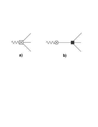
Figure 2: New diagrams due to the short-distance ${\cal O}(p^{4})$ operators $L_{1,2,3}^{SD}$. For a more detailed explanation, see the text. The vertices from $\mathcal{L}_{\rm non-R}^{(4)}$ ($\mathcal{L}_{\rm non-R}^{(2)}$) are represented by squares (circles). The straight lines are pions and the wavy ones correspond to the incoming $W^{-}$.

We will assume the ideal mixing in the tensor nonet $T_{\mu\nu}=T^{a}_{\mu\nu}\lambda^{a}/\sqrt{2}$ and that the $f_{2}(1270)$ resonance is the pure $u\bar{u}+d\bar{d}$ component:

$$T^{\mu\nu} = \left(\begin{array}[]{ccc}\frac{\displaystyle f_{2}^{\mu\nu}}{\displaystyle\sqrt{2}}&0&0\\ 0&\frac{\displaystyle f_{2}^{\mu\nu}}{\displaystyle\sqrt{2}}&0\\ 0&0&0\end{array}\right)\quad+\quad...$$ (40)

4.2 AFF into $T\pi^{-}$

The general possible structure for the hadronic matrix element into a tensor and a pion is given by three independent form-factors Castro:2011zd , which can be arranged in the form

$$\langle\,f_{2}(k,\epsilon)\,\pi^{-}(p_{3})|\,\bar{d}\gamma^{\alpha}\gamma_{5}u\,|0\,\rangle = \epsilon_{\mu\nu}^{*}H^{\alpha,\,\mu\nu}_{T\pi}$$

$$=i\,\epsilon_{\mu\nu}^{*}\,\left[P_{T}(q)^{\alpha\rho}\,p_{3}^{\nu}\,\left(\,g_{\rho}^{\mu}\,\mathcal{F}^{a}_{T\pi}(q^{2};k^{2})\,\,+\,\,p_{3\,\rho}p_{3}^{\mu}\,\mathcal{G}^{a}_{T\pi}(q^{2};k^{2})\,\right)\,\,+\,\,p_{3}^{\mu}p_{3}^{\nu}q^{\alpha}\,\mathcal{H}^{a}_{T\pi}(q^{2};k^{2})\right]\,,$$

with $q=p_{3}+k$ and $\epsilon_{\mu\nu}$ the polarization of the outgoing tensor Castro:2011zd ; Zauner:2007 . Due to the partial conservation of the axial-vector current, the $\mathcal{H}^{a}_{T\pi}(q^{2};k^{2})$ form-factor is suppressed by $m_{\pi}^{2}$.

Here the tensor resonance has been assumed to be the asymptotic final state with polarizations fulfilling the on-shell constraints Zauner:2007

$$\epsilon_{\mu\nu}=\epsilon_{\nu\mu}\,,\qquad k^{\mu}\epsilon_{\mu\nu}=0\,,\qquad g^{\mu\nu}\epsilon_{\mu\nu}=0\,.$$ (42)

We used the completeness relation Zauner:2007 ; LopezCastro:1997im

$$\!\!\!\!\!\!\!\!\mathcal{P}(k)^{\mu\nu,\alpha\beta}=\sum_{\epsilon}\epsilon_{\mu\nu}\epsilon^{*}_{\alpha\beta} = \frac{\displaystyle 1}{\displaystyle 2}\left(P(k)^{\mu\alpha}P(k)^{\nu\beta}+P(k)^{\nu\alpha}P(k)^{\mu\beta}\right)-\frac{\displaystyle 1}{\displaystyle 3}P(k)^{\mu\nu}P(k)^{\alpha\beta}\,\,$$ (43)

with $P(k)_{\mu\nu}=\left.P_{T}(k)^{\mu\nu}\right|_{k^{2}=M_{T}^{2}}=g_{\mu\nu}-k_{\mu}k_{\nu}/M_{T}^{2}$.

The hadronic Lagrangian from Eqs. (33) and (34) leads to the determination

$$\mathcal{F}^{a}_{T\pi}(q^{2};k^{2}) = -\frac{\displaystyle 8g_{T}}{\displaystyle F_{\pi}}+\frac{\displaystyle 4\sqrt{2}F_{A}\lambda_{1}^{AT}}{\displaystyle F_{\pi}}\frac{\displaystyle(qp_{3})}{\displaystyle M_{A}^{2}-q^{2}}-\frac{\displaystyle 2\sqrt{2}F_{A}\lambda_{2}^{AT}}{\displaystyle F_{\pi}}\frac{\displaystyle(qk)}{\displaystyle M_{A}^{2}-q^{2}}\,,$$

$$\mathcal{G}^{a}_{T\pi}(q^{2};k^{2}) = -\frac{\displaystyle 4\sqrt{2}F_{A}\lambda_{1}^{AT}}{\displaystyle F_{\pi}}\frac{\displaystyle 1}{\displaystyle M_{A}^{2}-q^{2}}-\frac{\displaystyle 2\sqrt{2}F_{A}\lambda_{2}^{AT}}{\displaystyle F_{\pi}}\frac{\displaystyle 1}{\displaystyle M_{A}^{2}-q^{2}}\,,$$

$$\mathcal{H}^{a}_{T\pi}(q^{2};k^{2}) = 0\,,$$ (44)

with $(qp_{3})=(q^{2}+m_{\pi}^{2}-k^{2})/2$ and $(qk)=(q^{2}-m_{\pi}^{2}+k^{2})$. Even though $k^{2}=M_{T}^{2}$ when the tensor resonance is on-shell we have kept the off-shell momentum dependence stemming from our R$\chi$T Lagrangian. The $m_{\pi}^{2}$ chiral suppressed form-factor $\mathcal{H}^{a}_{T\pi}(q^{2})$ is exactly zero in our approach as we are considering a resonance Lagrangian with the lowest number of derivatives (this is, two derivatives, ${\cal O}(p^{2})$) and the Lorentz structure corresponding to $\mathcal{H}^{a}_{T\pi}(q^{2};k^{2})$ carries three powers of external momenta.

If one imposes a vanishing behaviour for the contribution of the $T\pi$ absorptive cut to the axial-vector correlator at $q^{2}\to\infty$ one finds that the form-factors vanish at large momentum transfer like $\mathcal{F}^{a}_{T\pi}(q^{2};M_{T}^{2})\stackrel{{\scriptstyle q^{2}\to\infty}}{{\longrightarrow}}{\cal O}(1/q^{2})$ and $\mathcal{G}^{a}_{T\pi}(q^{2};M_{T}^{2})\stackrel{{\scriptstyle q^{2}\to\infty}}{{\longrightarrow}}{\cal O}(1/q^{4})$ or faster (see App. B for details). Demanding this to the previous R$\chi$T form-factors $\mathcal{F}^{a}_{T\pi}$ and $\mathcal{G}^{a}_{T\pi}$ yields, respectively, the constraints (taking into account $k^{2}=M_{T}^{2}$ for the on-shell resonance),

$$4\sqrt{2}g_{T}\,+\,2F_{A}\lambda_{1}^{AT}\,-\,F_{A}\lambda_{2}^{AT} = 0\,,\qquad\qquad 2\lambda_{1}^{AT}\,+\,\lambda_{2}^{AT}\,=\,0\,.$$ (45)

This leads to the resonance coupling relations

$$F_{A}\lambda_{2}^{AT} = -2F_{A}\lambda_{1}^{AT}\,=\,2\sqrt{2}g_{T}\,$$ (46)

and the form-factors

$$\mathcal{F}^{a}_{T\pi}(q^{2};k^{2}) = -\frac{\displaystyle 8g_{T}}{\displaystyle F_{\pi}}\frac{\displaystyle M_{A}^{2}}{\displaystyle M_{A}^{2}-q^{2}}\,,$$

$$\mathcal{G}^{a}_{T\pi}(q^{2};k^{2}) = 0\,.$$ (47)

This result agrees with that in Ref. Castro:2011zd near the axial-vector resonance. Furthermore, in the chiral limit, if one requires the same fall-off for the form-factors therein one has an agreement in the full energy range. Additional details can be found in App. C.2.

4.3 $3\pi$ AFF through an intermediate tensor resonance

The three possible decay mechanisms involving the tensor resonance are drawn in Fig. 1. We present here some useful intermediate results.

The $\pi^{0}\pi^{0}\pi^{-}$ production with the neutral pions mediated by a tensor resonance is provided by three ingredients:

• The transition $W^{-\mu}(q)\to f_{2}(k)^{*}\pi^{0}(p_{3})$ taking into account the three diagrams is given by

  $$\langle\,f_{2}^{*}(k,\epsilon)\pi^{-}(p_{3})|\bar{d}\gamma^{\mu}\gamma_{5}u|0\,\rangle\,=\,\epsilon_{\alpha\beta}^{*}H^{\mu,\,\alpha\beta}_{T\pi}$$ (48)

  $$\qquad=\,\frac{-4\sqrt{2}\,i}{F_{\pi}}p_{3}^{\alpha}\epsilon^{\star\alpha\beta}\Bigl{[}\sqrt{2}g_{T}\left(g_{\beta\mu}-\frac{q_{\beta}q_{\mu}}{q^{2}-m_{\pi}^{2}}\right)$$

  $$\qquad\qquad\qquad\qquad\qquad-F_{A}\frac{\left[\lambda_{1}^{AT}(qp_{3}g_{\beta\mu}-q_{\beta}p_{3\mu})\,-\,\frac{1}{2}\lambda_{2}^{AT}(qkg_{\beta\mu}-q_{\beta}k_{\mu})\right]}{M_{A}^{2}-q^{2}}\Bigr{]}\,.$$

  After imposing the high-energy constraints (46), this expression gets greatly simplified into

  $$H^{\mu,\,\alpha\beta}_{T\pi} = \frac{-8\,ig_{T}}{F_{\pi}}p_{3}^{\alpha}\Bigl{[}\frac{M_{A}^{2}}{M_{A}^{2}-q^{2}}\,P_{T}(q)^{\beta\mu}\,-\,\frac{\displaystyle m_{\pi}^{2}q_{\beta}q_{\mu}}{\displaystyle q^{2}(q^{2}-m_{\pi}^{2})}\Bigr{]}\,.$$ (49)

  We remark that we have not used the on-shell conditions in Eqs. (48) and (49) above.

• The tensor propagator Zauner:2007 :

  $$\Delta_{T}(k)^{\mu\nu,\alpha\beta} = \frac{\displaystyle i\,\mathcal{P}(k)^{\mu\nu,\alpha\beta}}{\displaystyle M_{T}^{2}-k^{2}}\,.$$ (50)

• The decay amplitude $\mathcal{M}(f_{2}^{*}(k)\to\pi^{0}(p_{1})\pi^{0}(p_{2}))=\epsilon^{\alpha\beta}\Gamma_{\alpha\beta}$ is given by

  $$\Gamma_{\alpha\beta} = \frac{-i\sqrt{2}g_{T}}{F_{\pi}^{2}}\Bigl{[}k^{\alpha}k^{\beta}-\Delta p^{\alpha}\,\Delta p^{\beta}\Bigr{]}\,,$$ (51)

  with $\Delta p^{\rho}=p_{1}^{\rho}-p_{2}^{\rho}$ and $k^{2}=s_{3}$. No on-shell condition has been assumed in the expression above. The term $k^{\alpha}k^{\beta}$ becomes zero when contracted with the $\epsilon^{\alpha\beta}$ polarization of an external on-shell tensor resonance.

The $\pi^{0}\pi^{0}\pi^{-}$ AFF is then given by

$$H^{\mu} = H_{(0)}^{\mu}\,+\,H_{T\pi}(k,p_{3})^{\mu,\,\alpha\beta}\,\,\,\Delta_{T}(k)_{\alpha\beta,\rho\sigma}\,\,\,\Gamma(p_{1},p_{2})^{\rho\sigma}$$

$$\,\,\,=\,\,\,H^{\mu}_{(0)}\,\,\,+\,\,\,H^{\mu}_{(1)}+\frac{H^{\mu}_{(2)}}{M_{T}^{2}-s_{3}}\,.$$

The first term, $H_{(0)}^{\mu}$, comes from the non-resonant diagrams in Fig. 2 generated by the short-distance terms $L_{1,2,3}^{SD}$ in Eqs. (35) and (36). The second and third ones, $H_{(1)}^{\mu}$ and $H_{(2)}^{\mu}$, respectively, are produced by the diagrams with tensor resonance exchanges (Fig. 1). $H_{(1)}^{\mu}$ comes from the $k^{\alpha}k^{\beta}$ term in the $\Gamma[T(k)_{\alpha\beta}\to\pi^{0}(p_{1})\pi^{0}(p_{2})]$ vertex function and does not contribute to the on-shell decay $T\to\pi^{0}\pi^{0}$. For sake of this, the contribution with $H_{(1)}^{\mu}$ does not propagate the tensor resonance and has no pole at $s_{3}=M_{T}^{2}$. The contribution to the three-pion AFF from the remaining part of the $T\pi^{0}\pi^{0}$ vertex is encoded in $H_{(2)}^{\mu}$.

The value of these two types of contributions are

$$H^{\mu}_{(0)} = \frac{\displaystyle 8\sqrt{2}ig_{T}^{2}}{\displaystyle 3F_{\pi}^{3}M_{T}^{2}}P_{T}(q)^{\mu\nu}\big{[}(s_{3}-s_{2}+2s_{1}-4m_{\pi}^{2})(p_{1}-p_{3})_{\nu}$$

$$\qquad\qquad\qquad\qquad\qquad+(s_{3}-s_{1}+2s_{2}-4m_{\pi}^{2})(p_{2}-p_{3})_{\nu}\big{]}$$

$$-\frac{\displaystyle 8\sqrt{2}ig_{T}^{2}m_{\pi}^{2}}{\displaystyle F_{\pi}^{3}M_{T}^{2}q^{2}(q^{2}-m_{\pi}^{2})}\,q^{\mu}\,\left(s_{1}s_{2}-m_{\pi}^{2}q^{2}-m_{\pi}^{4}\right)$$

$$H^{\mu}_{(1)} = \frac{\displaystyle 8\sqrt{2}ig_{T}^{2}}{\displaystyle F_{\pi}^{3}M_{T}^{2}}\frac{\displaystyle m_{\pi}^{2}}{\displaystyle q^{2}(q^{2}-m_{\pi}^{2})}\,q^{\mu}\,\left[(kq)(kp_{3})-\frac{s_{3}}{3}\left((qp_{3})+\frac{\displaystyle 2(kq)(kp_{3})}{\displaystyle M_{T}^{2}}\right)\right]$$

$$-\,\frac{\displaystyle 8ig_{T}}{\displaystyle F_{\pi}^{3}M_{T}^{2}}\frac{\displaystyle M_{A}^{2}}{\displaystyle(M_{A}^{2}-q^{2})}P_{T}(q)^{\mu\nu}k_{\nu}\bigg{[}\sqrt{2}g_{T}\left(\left(1-\frac{\displaystyle 2s_{3}}{\displaystyle 3M_{T}^{2}}\right)(kp_{3})+\frac{\displaystyle s_{3}}{\displaystyle 3}\right)$$

$$\qquad+(F_{A}\lambda_{1}^{AT}+\sqrt{2}g_{T})\frac{\displaystyle q^{2}(kp_{3})}{\displaystyle M_{A}^{2}}\,\left(\frac{\displaystyle 2s_{3}}{\displaystyle 3M_{T}^{2}}-1\right)+(F_{A}\lambda_{2}^{AT}-2\sqrt{2}g_{T})\frac{\displaystyle q^{2}s_{3}}{\displaystyle 6M_{A}^{2}}\bigg{]}\,,$$

$$H^{\mu}_{(2)\,{\rm a_{1}-pole}} = -\,\frac{\displaystyle 8ig_{T}}{\displaystyle F_{\pi}^{3}}\frac{\displaystyle F_{A}}{\displaystyle M_{A}^{2}-q^{2}}P_{T}(q)^{\mu\nu}\bigg{[}\left(\lambda_{1}^{AT}M_{A}^{2}-\left(\lambda_{1}^{AT}+\frac{\displaystyle\lambda_{2}^{AT}}{\displaystyle 2}\right)(kq)\right)\,(q\Delta p)\,\Delta p_{\nu}$$ (55)

$$+\left(\frac{\displaystyle\lambda_{1}^{AT}M_{A}^{2}(\Delta p)^{2}(kp_{3}+M_{T}^{2})}{\displaystyle 3M_{T}^{2}}+\left(\lambda_{1}^{AT}+\frac{\displaystyle\lambda_{2}^{AT}}{\displaystyle 2}\right)\left((q\Delta p)^{2}-\frac{\displaystyle(\Delta p)^{2}M_{A}^{2}}{\displaystyle 3}\right)\right)k^{\nu}\bigg{]}\,,$$

$$H^{\mu}_{(2)\,{\rm a_{1}\,no-pole}} = -\,\frac{\displaystyle 2\sqrt{2}ig_{T}}{\displaystyle F_{\pi}^{3}}P_{T}(q)^{\mu\nu}\bigg{[}-2\sqrt{2}(F_{A}\lambda_{1}^{AT}+\sqrt{2}g_{T})\left((q\Delta p)\Delta p_{\nu}+\frac{\displaystyle(kp_{3})(\Delta p)^{2}}{\displaystyle 3M_{T}^{2}}k_{\nu}\right)$$ (56)

$$+\sqrt{2}(F_{A}\lambda_{2}^{AT}-2\sqrt{2}g_{T})\frac{\displaystyle(\Delta p)^{2}}{\displaystyle 3}k_{\nu}\bigg{]}$$

$$-\,\frac{\displaystyle 8\sqrt{2}ig_{T}^{2}m_{\pi}^{2}}{\displaystyle F_{\pi}^{3}q^{2}(q^{2}-m_{\pi}^{2})}\,q^{\mu}\,\bigg{[}(q\Delta p)^{2}+\frac{\displaystyle(\Delta p)^{2}}{\displaystyle 3M_{T}^{2}}\left(kq\,kp_{3}-qp_{3}M_{T}^{2}\right)\bigg{]}\,,$$

with $(\Delta p)^{2}=4m_{\pi}^{2}-s_{3}$, $(kq)=(q^{2}+s_{3}-m_{\pi}^{2})/2$ and $(k\Delta p)=0$. From these, one can derive a series of dependent scalars: $(kp_{3})=(qk)-s_{3}=(q^{2}-s_{3}-m_{\pi}^{2})/2$, $(qp_{3})=q^{2}-(qk)=(q^{2}-s_{3}+m_{\pi}^{2})/2$, $(q\Delta p)=(p_{3}\Delta p)=(s_{2}-s_{1})/2$ and the relation $s_{1,2}=kp_{3}+2m_{\pi}^{2}\mp q\Delta p$. For convenience we have split $H^{\mu}_{(2)}$ into its parts with and without the $a_{1}$ pole. We also used the relation $(qp_{3})k^{\mu}-(qk)p_{3}^{\mu}=q^{2}P_{T}(q)^{\mu\nu}k_{\nu}$.

We now combine $H_{(0)}^{\mu}$, $H_{(1)}^{\mu}$ and $H_{(2)}^{\mu}$ and rewrite their sum in terms of the Lorentz decomposition (1). This provides the contribution to the ${\pi^{0}\pi^{0}\pi^{-}}$ AFFs in (1) derived from tensor resonance exchanges:

$$\mathcal{F}_{1}^{\pi^{0}\pi^{0}\pi^{-}}(s_{1},s_{2},q^{2})\bigg{|}_{T} = \mathcal{F}_{1,\,\,(0)}^{\pi^{0}\pi^{0}\pi^{-}}(s_{1},s_{2},q^{2})\,+\,\mathcal{F}^{\pi^{0}\pi^{0}\pi^{-}}_{1,\,\,\rm(RSD)}(s_{1},s_{2},q^{2})$$

$$-\frac{\displaystyle 4}{\displaystyle 9F_{\pi}^{3}}\frac{\displaystyle g_{T}}{\displaystyle M_{T}^{2}}\frac{\displaystyle(F_{A}\lambda_{2}^{AT}-2\sqrt{2}g_{T})}{\displaystyle M_{A}^{2}-q^{2}}\times\bigg{[}s_{3}q^{2}$$

$$\qquad+\frac{\displaystyle M_{T}^{2}}{\displaystyle M_{T}^{2}-s_{3}}\left(3(q\Delta p)^{2}-9(qk)(q\Delta p)-q^{2}(\Delta p)^{2}\right)\bigg{]}$$

$$-\frac{\displaystyle 8}{\displaystyle 3F_{\pi}^{3}}\frac{\displaystyle g_{T}}{\displaystyle M_{T}^{2}}\frac{\displaystyle(F_{A}\lambda_{1}^{AT}+\sqrt{2}g_{T})}{\displaystyle M_{A}^{2}-q^{2}}\times\bigg{[}q^{2}(kp_{3})\left(\frac{\displaystyle 2s_{3}}{\displaystyle 3M_{T}^{2}}-1\right)$$

$$\qquad+\frac{\displaystyle M_{T}^{2}}{\displaystyle M_{T}^{2}-s_{3}}\left((q\Delta p)^{2}+3(q\Delta p)(qp_{3})+\frac{\displaystyle q^{2}(kp_{3})(\Delta p)^{2}}{\displaystyle 3M_{T}^{2}}\right)\bigg{]}$$

$$\mathcal{F}_{P}^{\pi^{0}\pi^{0}\pi^{-}}(s_{1},s_{2},q^{2})\bigg{|}_{T} = \mathcal{F}_{P,\,\,(0)}^{\pi^{0}\pi^{0}\pi^{-}}(s_{1},s_{2},q^{2})\,$$

$$+\frac{8\sqrt{2}g_{T}^{2}m_{\pi}^{2}}{3M_{T}^{2}F_{\pi}^{3}q^{2}(m_{\pi}^{2}-q^{2})}\times\bigg{[}(qp_{3})s_{3}+(kq)(kp_{3})\left(\frac{\displaystyle 2s_{3}}{\displaystyle M_{T}^{2}}-3\right)$$

$$\qquad+\frac{\displaystyle M_{T}^{2}}{\displaystyle M_{T}^{2}-s_{3}}\left(3(q\Delta p)^{2}+\left(\frac{\displaystyle(kq)(kp_{3})}{\displaystyle M_{T}^{2}}-(qp_{3})\right)(\Delta p)^{2}\right)\Bigg{]}\,,$$

with

$$\mathcal{F}_{1,\,\,(0)}^{\pi^{0}\pi^{0}\pi^{-}}(s_{1},s_{2},q^{2}) = \frac{\displaystyle 8\sqrt{2}g_{T}^{2}}{\displaystyle 3F_{\pi}^{3}M_{T}^{2}}(2s_{1}-s_{2}+s_{3}-4m_{\pi}^{2})\,,$$ (59)

$$\mathcal{F}_{P,\,\,(0)}^{\pi^{0}\pi^{0}\pi^{-}}(s_{1},s_{2},q^{2}) = -\frac{\displaystyle 8\sqrt{2}g_{T}^{2}m_{\pi}^{2}}{\displaystyle F_{\pi}^{3}M_{T}^{2}q^{2}(q^{2}-m_{\pi}^{2})}\left(s_{1}s_{2}-m_{\pi}^{2}q^{2}-m_{\pi}^{4}\right)\,,$$ (60)

$$\mathcal{F}^{\pi^{0}\pi^{0}\pi^{-}}_{1,\,\,\rm(RSD)}(s_{1},s_{2},q^{2}) = -\frac{\displaystyle 8\sqrt{2}}{\displaystyle 3F_{\pi}^{3}}\frac{\displaystyle g_{T}^{2}}{\displaystyle M_{T}^{2}}\frac{\displaystyle M_{A}^{2}}{\displaystyle M_{A}^{2}-q^{2}}\bigg{[}(kp_{3})+\frac{\displaystyle s_{3}}{\displaystyle 3}\left(1-\frac{\displaystyle 2(kp_{3})}{\displaystyle M_{T}^{2}}\right)$$ (61)

$$\qquad-\frac{\displaystyle M_{T}^{2}}{\displaystyle M_{T}^{2}-s_{3}}\left(3(q\Delta p)+\frac{\displaystyle(\Delta p)^{2}}{\displaystyle 3}+\frac{\displaystyle(kp_{3})(\Delta p)^{2}}{\displaystyle 3M_{T}^{2}}\right)\bigg{]}\,,$$

where the contributions $\mathcal{F}_{1,\,\,(0)}^{\pi^{0}\pi^{0}\pi^{-}}$ and $\mathcal{F}_{P,\,\,(0)}^{\pi^{0}\pi^{0}\pi^{-}}$ come from the $H_{(0)}^{\mu}$ part of the matrix element $H^{\mu}$.

All the results here refer to the $\pi^{0}\pi^{0}\pi^{-}$ AFF. Isospin symmetry Pais:1960zz ; Finkemeier:1996 ; Girlanda:1999fu relates them to the $\pi^{-}\pi^{-}\pi^{+}$ form-factors, which can be obtained by mean of the relations (5).

The expression of the form-factors get greatly simplified after applying the high-energy constraints extracted from the analysis of the $T\pi$ AFF in Eq. (46):

$$\mathcal{F}_{1}^{\pi^{0}\pi^{0}\pi^{-}}(s_{1},s_{2},q^{2})\bigg{|}_{T} = \mathcal{F}_{1,\,\,(0)}^{\pi^{0}\pi^{0}\pi^{-}}(s_{1},s_{2},q^{2})\,+\,\mathcal{F}^{\pi^{0}\pi^{0}\pi^{-}}_{1,\,\,\rm(RSD)}(s_{1},s_{2},q^{2})\,,$$ (62)

while these resonance short-distance conditions do not affect the longitudinal form-factor $\mathcal{F}_{P}(s_{1},s_{2},q^{2})\bigg{|}_{T}$, which remains the same as in (4.3).

The comparison between CLEO’s results and ours for the amplitude and the related AFF is given in App. C.1. From that, we conclude that the two parametrizations coincide near the resonance energy regions ($s_{3}\simeq M_{T}^{2}$, $q^{2}\simeq M_{A}^{2}$). However, for an arbitrary off-shell momentum we have a more general momentum structure which ensures the right low energy behaviour and the transversality of the matrix element in the chiral limit, allowing a proper matching with $\chi$PT.

4.4 Tensor resonance width

In order to include the effect of the tensor width, we modify the tensor resonance propagator in the form

$$\frac{1}{M_{T}^{2}-s}\qquad\longrightarrow\qquad\frac{1}{M_{f_{2}}^{2}-s-iM_{f_{2}}\Gamma_{f_{2}}(s)}\,,$$ (63)

with the spin–2 energy-dependent Breit-Wigner width used in CLEO’s analysis CLEO:1999 ,

$$\Gamma_{f_{2}}(s) = \,\Gamma^{f_{2}}_{0}\,\frac{\displaystyle s^{2}}{\displaystyle M_{f_{2}}^{4}}\,\frac{\displaystyle\rho_{\pi}(s)^{5}}{\displaystyle\rho_{\pi}(M_{f_{2}}^{2})^{\,5}}\,\,.$$ (64)

For the numerical estimation in the next Section we will take the PDG central value $\Gamma^{f_{2}}_{0}=186.7$ MeV for the $f_{2}(1270)$ total decay width pdg .

The tensor contribution to the AFF depends on the $g_{T}$ coupling, which is related to the on-shell decay width into two pseudo-Goldstones Zauner:2007 :

$$\Gamma_{f_{2}\to\pi\pi} = \frac{\displaystyle g_{T}^{2}M_{f_{2}}^{3}\rho_{\pi}(M_{f_{2}}^{2})^{\,5}}{\displaystyle 40\pi F_{\pi}^{4}}\,.$$ (65)

Using the PDG central values, $\Gamma_{f_{2}\to\pi\pi}^{\rm exp}=157.2$ MeV, $M_{f_{2}}=1275.5$ MeV, $m_{\pi}=139.57$ MeV and $F_{\pi}=92.2$ MeV, one obtains

$$g_{T}\simeq 28\,\mbox{MeV}\,,$$ (66)

which agrees with the estimation in Zauner:2007 .

5 Implementation in Tauola: numerical results

In the previous sections we described the set of the three pion form factor contributions related with the tensor and scalar intermediate resonances and calculated on the base of the R$\chi$T Lagrangians. In this section we present a first numerical estimate with the updated version of the Monte Carlo (MC) event generator Tauola Jadach:1993hs . It incorporates the new scalar and tensor contributions to the AFF computed in this article, provided in (22) and (4.3), respectively.

First, we compare the analytical and Tauola distributions for the decay width ($d\Gamma^{\pi\pi\pi}/dq^{2}$) and repeat the tests on numerical stability of the MC, as in Sec. 4 of Ref. Shekhovtsova:2012ra   For further details see this reference. The comparison is presented in Fig. 3. We present here only $d\Gamma^{\pi^{0}\pi^{0}\pi^{-}}/dq^{2}$ spectrum. A similar result has been obtained for the $\pi^{-}\pi^{-}\pi^{+}$ mode.

Figure 3: Three pion $q^{2}$ spectrum $d\Gamma^{\pi^{0}\pi^{0}\pi^{-}}/dq^{2}$ (left) and the ratio of the MC and the analytical $q^{2}$ spectrum (right).

In addition we have compared the two- and three-meson invariant mass distributions for our theoretical result and the experimental data. For the $\pi^{-}\pi^{-}\pi^{+}$ channel, we used preliminary BaBar data Nugent:2013ij (Fig. 4, top panels). Due to our lack of access to the $\pi^{0}\pi^{0}\pi^{-}$ data, they have been ’emulated’ on the basis of the results in Ref. CLEO:1999 : Tauola was run with CLEO’s AFF from App. A.1 of CLEO:1999 and nominal fit parameters specified therein in Table III.  The comparison of our parametrization to this ‘emulation’ of CLEO data is shown in Fig. 4, bottom panel.

To produce the theoretical distributions the tensor and scalar resonance parameters were fixed to their value specified in Secs. 3.4 and 4.4 whereas the vector and axial-vector parameters were fixed to their fit values in Nugent:2013hxa . All parameters are summarized in Table 1 except $c_{m}$. This coupling, whose effects are suppressed by $m_{\pi}^{2}$ factors, is extracted from the $c_{d}$ and $F_{\pi}$ values in Table 1 and the short-distance constraint $4c_{d}c_{m}=F_{\pi}^{2}$ Jamin:2001zq .

Table 1: Numerical values of the parameters used to produce the theoretical spectra in 4. All the parameters are in GeV units except for $c_{\sigma}$ and $c_{f_{0}}$, which are dimensionless.

$M_{\rho}$	$M_{\rho^{\prime}}$	$\Gamma_{\rho^{\prime}}$	$M_{a_{1}}$	$M_{\sigma}$	$M_{f_{2}}$	$\Gamma_{f_{2}}$	$F_{\pi}$
$0.772$	$1.35$	$0.448$	$1.10$	$0.8064$	$1.275$	$0.185$	$0.0922$

$F_{V}$	$F_{A}$	$\beta_{\rho}$	$g_{T}$	$c_{d}$	$c_{\sigma}$	$M_{f_{0}}$	$c_{f_{0}}$
$0.168$	$0.131$	$-0.32$	$0.028$	$0.026$	$76.12$	$1.024$	$17.7$

These plots in Fig. 4 are an illustration of our model, which demonstrates that, even without fitting, the model qualitatively reproduces the experimental spectra. No large unwanted deviation from data occurs, being these values an appropriate starting point for a more detailed study. The tuning of our model parameters and the fitting to the data will be done in a future work new-paper-fit .

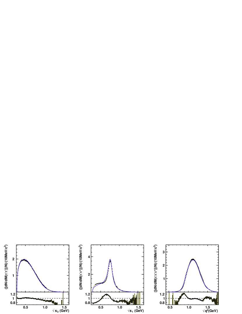
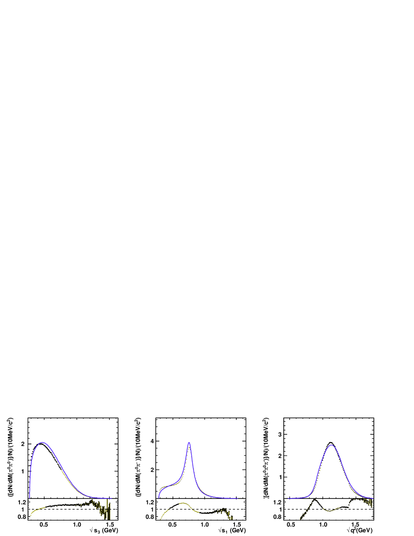
Figure 4: Top: comparison between the BaBar data and our theoretical prediction for the $\pi^{-}\pi^{-}\pi^{+}$ decay mode. Bottom: comparison between the CLEO ’emulated’ data (for details the text) and our prediction for the $\pi^{0}\pi^{0}\pi^{-}$ decay mode.

In order to understand the impact of the different contributions we focus our attention in the $\pi^{0}\pi^{0}\pi^{-}$ channel, where the various contributions are more neatly separated: vectors only resonate in the $s_{1}$ and $s_{2}$ spectra, and scalars and tensors only resonate in the $s_{3}$ distribution. The first thing to notice is that all the distributions are dominated by the vector contribution “$V$” (Lagrangian with only chiral Goldstones, vectors and axial-vectors Dumm:2009va ; Shekhovtsova:2012ra ). The scalar resonances (in particular the $\sigma$ meson) serve to cure the discrepancies with respect to the data that appear in the low energy regions, $M_{\pi\pi}<M_{\rho}$ Nugent:2013hxa . In Fig. 5 we show the ratio of our theoretical $\sqrt{s_{3}}$ distribution including only the vector contribution $V$ Nugent:2013hxa ) and its full result ($V+S+T$) in Fig. 4 (all with the inputs given in Table 1). For this set of parameters, we find that the scalar corrections are smaller than 10% in the low-energy region. Therefore, when fitting the experimental data in this range, we will find that small variations in the vector parameters may compensate large modifications in the scalar ones, being highly correlated for this observable. Finally, the tensor resonance produces in general a negligible effect in all the distributions except in the $\sqrt{s_{3}}$ one around 1.25 GeV, where one can observe the clear emergence of the $f_{2}(1270)$ structure in Fig. 5.

Figure 5: a) Ratio of the vector+tensor+scalar and only vector $\sqrt{s_{3}}=M_{\pi^{0}\pi^{0}}$ spectral function for $\tau\to\nu_{\tau}\pi^{0}\pi^{0}\pi^{-}$; b) Ratio of vector+scalar and only vector; c) Ratio of vector+tensor and only vector. All the plots use the inputs in Table 1 ($c_{d}=26$ MeV).

Figure 6: a) Ratio of the vector+tensor+scalar and only vector $\sqrt{s_{3}}=M_{\pi^{0}\pi^{0}}$ spectral function for $\tau\to\nu_{\tau}\pi^{0}\pi^{0}\pi^{-}$; b) Ratio of vector+scalar and only vector. All the plots use the inputs in Table 1 except for $c_{d}$, which is set to $78$ MeV. The ratio vector+tensor/vector is independent of $c_{d}$ and is provided in Fig. 5.c.

All the former analyses in this article are performed for the $S\pi\pi$ coupling $c_{d}=26$ MeV in Table 1. It is not clear whether this is the most suitable value, as other studies do not lead to a conclusive estimate, allowing a much higher coupling Sdecays . Since the scalar contribution to the amplitude is essentially proportional to $c_{d}^{2}$, multiplying the value of $c_{d}$ by a factor 3 increases the impact of the scalar in the spectral function by one order of magnitude (through the interference with the $V$ contribution). For illustration, in Fig. 6, we show the same ratio as in Fig. 5 but for $c_{d}=78$ MeV. The impact of these variations can be as important as small modifications of the $V$ parameters. Thus, it is not possible to pin down the scalar couplings without an accurate determination of the vector ones. A joint fit is mandatory.

Another important numerical issue refers to the relevance of the real part of the logarithm that is incorporated to the $\sigma$ propagator à la Gounaris-Sakurai. In Fig. 7.a (Fig. 7.b) we show the ratio of our theoretical $\sqrt{s_{3}}$ distribution neglecting the real part of the $\sigma$ logs in Eqs. (28)–(29) and the full results from these equations for $c_{d}=26$ MeV ($c_{d}=78$ MeV). For all the other parameters we use the inputs from Table 1 and take only the vector+scalar contributions for sake of clarity. Since the scalar contribution is quite small, the impact of the real logs of the $\sigma$ propagator in the full spectral distributions is quite suppressed for this $\tau$ decay. We want to emphasize that although a Breit-Wigner $\sigma$ can provide an equally good description of the data Nugent:2013hxa , the aim of the present analysis of the $\sigma$ à la Gounaris-Sakurai is rather to improve the theoretical understanding of broad resonances within a Lagrangian formalism and its matching to $\chi$PT at low energies.

Figure 7: Plots for the ratios of the $\sqrt{s_{3}}=M_{\pi^{0}\pi^{0}}$ spectral functions for $\tau\to\nu_{\tau}\pi^{0}\pi^{0}\pi^{-}$: a) ratio of the full result and the spectral function without the real part of the logs in the $\sigma$ propagator for $c_{d}=26$ MeV; b) ratio of the full result and the spectral function without the real part of the logs in the $\sigma$ propagator for $c_{d}=78$ MeV. In order to better pin down the impact of the scalar propagator structure we only consider the vector+scalar contribution, dropping the tensors.

6 Conclusions

In this article we have computed the contribution of scalar and tensor resonances to the $\tau\to\pi\pi\pi\nu_{\tau}$ decay axial-vector form-factors. We have made use of a chiral invariant Lagrangian including the relevant axial-vector, scalar and tensor resonances together with the chiral (pseudo) Goldstones.

As a consequence of this, the chiral symmetry is automatically incorporated in our result. This ensures the proper low-energy matching with $\chi$PT and that the currents for $\pi^{0}\pi^{0}\pi^{-}$ and $\pi^{-}\pi^{-}\pi^{+}$ channels are related as prescribed by isospin symmetry Girlanda:1999fu ; Finkemeier:1996 . In addition, the tensor resonance contribution to the axial-vector current is transverse in the chiral limit, improving previous descriptions Castro:2011zd . A similar thing applies to the scalar contributions. Chiral symmetry also guaranties the proper low-energy matching with $\chi$PT, fixing some issues in former parametrizations CLEO:1999 (see App. C.1).

In addition, the tensor and scalar resonance contributions to the tau decay are further refined by demanding the appropriate asymptotic high-energy QCD behaviour for meson form-factors prescribed by the quark-counting rules Brodsky:1973kr . As described in Secs. 3.3, 4.2 and App. B, these large–$N_{C}$ short distance conditions constrain the resonance parameters of the $T\pi$ and $S\pi$ AFFs, which are essentially determined in terms of the $g_{T}$ and $c_{d}$ couplings, respectively, and the resonance masses.

We have also studied an alternative approach to the sigma description incorporating an analytical description of the width à la Gounaris-Sakurai GS-rho : instead of just the imaginary part $i\rho_{\pi}(s)$ required by unitarity in the K-matrix formalism or the Breit-Wigner form Nugent:2013hxa , we considered the full logarithm from the analytical Chew-Mandelstam dispersive integral Chew:1960iv or the renormalized two-propagator Feynman integral $\overline{B}_{0}$. This parametrization of the $\sigma$ propagator provided a successful description of the $\eta\textquoteright\to\eta\pi\pi$ data and its $s$–wave $\pi\pi$ rescattering Escribano:2010wt . Although it requires further refinements, we find the exploration of this approach for $\tau\to 3\pi\nu_{\tau}$ worthy, as it may help to understand whether it is possible or not to use a Lagrangian formalism based on a perturbative expansion ($1/N_{C}$ in our case) for the description of broad resonances.

We would like to note that in this article we have considered for the first time the axial-vector–tensor interaction within the Resonance Chiral Theory approach, extending the work of Ecker and Zauner on tensors Zauner:2007 . We plan to include vector–tensor interactions in a similar way in a future paper new-paper dedicated to the study of the $e^{+}e^{-}\to a_{2}\pi$ process.

We have compared our outcome for the $\pi\pi\pi$ AFF with former parametrizations with CLEO CLEO:1999 and Castro-Muñoz Castro:2011zd . While we coincide on the resonance region, our result incorporates an appropriate low and high-energy behaviour, improving these works in the latter regimes. As we plan to incorporate these new results in the Tauola generator, which generates events from the three pion threshold up to roughly the tau mass, it is important to handle as best as possible the various energy ranges (low, resonant and high). Some first simulations with the Tauola Monte Carlo have been provided in Sec. 5. This article is only a preliminary illustration of our resonance chiral Lagrangian approach. A more thorough numerical analysis is postponed for a future work new-paper-fit . In order to obtain a good fit to the BaBar data, we will probably need not only the one-dimensional distributions but also the Dalitz plot. A proper tuning of the Monte Carlo parameters (e.g., the $S\pi\pi$ coupling $c_{d}$) should be reading before the beginning of the Belle-II data taking.

To conclude: we would like to remind that the forthcoming project Belle-II Abe:2010gxa has a broad program devoted to $\tau$-physics. By 2022, they expect to record a $50$ times lager data sample than the Belle experiment. It will give us an opportunity to measure both $\pi^{-}\pi^{-}\pi^{+}$ and $\pi^{0}\pi^{0}\pi^{-}$ decays and study their intermediate production mechanisms like, e.g., the tiny contribution from the $f_{2}\pi^{-}$ channel. This will allow us to test our hadronic model and the isospin symmetry relation between $\pi^{-}\pi^{-}\pi^{+}$ and $\pi^{0}\pi^{0}\pi^{-}$ form factors.

Appendix A Axial-vector form-factor into $3\pi$ in $\chi$PT

In this Appendix, we will focus on the non-chirally suppressed form-factor $\mathcal{F}_{1}$. At tree-level, $\chi$PT gives the low-energy expansion up to ${\cal O}(p^{4})$ Finkemeier:1996  

$$\mathcal{F}_{1}^{\pi^{0}\pi^{0}\pi^{-}}(s_{1},s_{2},q^{2}) = \frac{\displaystyle 2\sqrt{2}}{\displaystyle 3F_{\pi}}\bigg{(}1\,+\,\frac{\displaystyle 4(2L_{1}+L_{3})}{\displaystyle F_{\pi}^{2}}(s_{3}-2m_{\pi}^{2})$$ (67)

$$\quad+\frac{\displaystyle 4L_{2}}{\displaystyle F_{\pi}^{2}}(s_{2}-2s_{1}+2m_{\pi}^{2})+\frac{\displaystyle 4(2L_{4}+L_{5})m_{\pi}^{2}}{\displaystyle F_{\pi}^{2}}+\frac{\displaystyle 2L_{9}q^{2}}{\displaystyle F_{\pi}^{2}}\bigg{)}\,,$$

with $q^{2}=(p_{1}+p_{2}+p_{3})^{2}$ and $s_{1}=(p_{2}+p_{3})^{2}$, etc. Notice the kinematical constraint $s_{1}+s_{2}+s_{3}=q^{2}+3m_{\pi}^{2}$.

At ${\cal O}(p^{2})$ the $\pi^{0}\pi^{0}\pi^{-}$ and $\pi^{-}\pi^{-}\pi^{+}$ channels are related through isospin in the simple form

$$\mathcal{F}_{1}^{\pi^{0}\pi^{0}\pi^{-}}(s_{1},s_{2},q^{2})\,=\,-\,\mathcal{F}_{1}^{\pi^{-}\pi^{-}\pi^{+}}(s_{1},s_{2},q^{2}) = \frac{\displaystyle 2\sqrt{2}}{\displaystyle 3F}\,.$$ (68)

Nonetheless, resonance contributions will show up at ${\cal O}(p^{4})$ and higher rcht ; op6rxt ; Zauner:2007 , in general spoiling this relation.

In the case when there are only vector contributions to the LECs one finds rcht ,

$$L_{2}\bigg{|}_{V}=2L_{1}\bigg{|}_{V}=-\frac{\displaystyle L_{3}}{\displaystyle 3}\bigg{|}_{V}=\frac{\displaystyle G_{V}^{2}}{\displaystyle 4M_{V}^{2}}\,,\qquad L_{9}\bigg{|}_{V}=\frac{\displaystyle F_{V}G_{V}}{\displaystyle 2M_{V}^{2}}\,,$$ (69)

with the remaining ${\cal O}(p^{4})$ LECs being zero. Thus, one has the ${\cal O}(p^{4})$ contribution Zuo:2013

$$\mathcal{F}_{1}^{\pi^{0}\pi^{0}\pi^{-}}(s_{1},s_{2},q^{2})\bigg{|}_{V}\,=\,-\,\mathcal{F}_{1}^{\pi^{-}\pi^{-}\pi^{+}}(s_{1},s_{2},q^{2})\bigg{|}_{V} = \frac{\displaystyle 2\sqrt{2}}{\displaystyle 3F}\left(\frac{\displaystyle 8L_{1}(3s_{2}-2q^{2})}{\displaystyle F^{2}}+\frac{\displaystyle 2L_{9}q^{2}}{\displaystyle F^{2}}\right)\bigg{|}_{V}\,.$$

The situation is different in the case when there are only scalar contributions to the ${\cal O}(p^{4})$ LECs rcht :

$$L_{1}\bigg{|}_{S}=\frac{\displaystyle\widetilde{c}_{d}^{2}}{\displaystyle 2M_{S_{1}}^{2}}-\frac{\displaystyle c_{d}^{2}}{\displaystyle 6M_{S}^{2}}\,,\qquad L_{2}\bigg{|}_{S}=L_{9}\bigg{|}_{S}=0\,,\qquad L_{3}\bigg{|}_{S}=\frac{\displaystyle c_{d}^{2}}{\displaystyle 2M_{S}^{2}}\,,$$

$$L_{4}\bigg{|}_{S}=\frac{\displaystyle\widetilde{c}_{d}\widetilde{c}_{m}}{\displaystyle M_{S_{1}}^{2}}-\frac{\displaystyle c_{d}c_{m}}{\displaystyle 3M_{S}^{2}}\,,\qquad L_{5}\bigg{|}_{S}=\frac{\displaystyle c_{d}c_{m}}{\displaystyle M_{S}^{2}}\,.$$ (71)

Taking this into account one obtains the ${\cal O}(p^{4})$ contribution

$$\mathcal{F}_{1}^{\pi^{0}\pi^{0}\pi^{-}}(s_{1},s_{2},q^{2})\bigg{|}_{S} = \frac{\displaystyle 2\sqrt{2}}{\displaystyle 3F_{\pi}}\bigg{(}\frac{\displaystyle 4(2L_{1}+L_{3})}{\displaystyle F_{\pi}^{2}}(s_{3}-2m_{\pi}^{2})+\frac{\displaystyle 4(2L_{4}+L_{5})m_{\pi}^{2}}{\displaystyle F_{\pi}^{2}}\bigg{)}\bigg{|}_{S}\,,$$

$$\mathcal{F}_{1}^{\pi^{-}\pi^{-}\pi^{+}}(s_{1},s_{2},q^{2})\bigg{|}_{S} = -\frac{\displaystyle 2\sqrt{2}}{\displaystyle 3F_{\pi}}\bigg{(}\frac{\displaystyle 4(2L_{1}+L_{3})}{\displaystyle F_{\pi}^{2}}(2s_{1}-s_{2}-2m_{\pi}^{2})+\frac{\displaystyle 4(2L_{4}+L_{5})m_{\pi}^{2}}{\displaystyle F_{\pi}^{2}}\bigg{)}\bigg{|}_{S}\,.$$

Except for the special point $s_{1}=(q^{2}+3m_{\pi}^{2})/3$, the $\mathcal{F}_{1}$ functions of the two decay channels have a different kinematical dependence and one cannot simply assume $\mathcal{F}_{1}^{\pi^{0}\pi^{0}\pi^{-}}(s_{1},s_{2},q^{2})\,=\,-\,\mathcal{F}_{1}^{\pi^{-}\pi^{-}\pi^{+}}(s_{1},s_{2},q^{2})$. This precise expression (A) can be directly obtained from the low-energy limit of Eq. (22),

$$\mathcal{F}_{1}^{\pi^{0}\pi^{0}\pi^{-}}(s_{1},s_{2},q^{2})\bigg{|}_{S} = \frac{4\sqrt{2}}{3F_{\pi}^{3}}\frac{1}{M_{S}^{2}}\,[c_{d}^{2}(s_{3}-2m_{\pi}^{2})+2c_{d}c_{m}m_{\pi}^{2}]\,,$$ (73)

where in the large $N_{C}$ limit the octet and singlet scalar couplings are related in the form $\widetilde{c}_{d}=c_{d}/\sqrt{3}$ and $\widetilde{c}_{m}=c_{m}/\sqrt{3}$, and $L_{1}|_{S}$ and $L_{4}|_{S}$ turn zero rcht .

Taking only the tensor resonance contribution, the ${\cal O}(p^{4})$ contributions to the form-factors become

$$\mathcal{F}_{1}^{\pi^{0}\pi^{0}\pi^{-}}(s_{1},s_{2},q^{2})\bigg{|}_{T} = \frac{\displaystyle 2\sqrt{2}}{\displaystyle 3F_{\pi}}\bigg{(}\frac{\displaystyle 4L_{3}}{\displaystyle F_{\pi}^{2}}(s_{3}-2m_{\pi}^{2})\bigg{)}\bigg{|}_{T}\,,$$

$$\mathcal{F}_{1}^{\pi^{-}\pi^{-}\pi^{+}}(s_{1},s_{2},q^{2})\bigg{|}_{T} = -\frac{\displaystyle 2\sqrt{2}}{\displaystyle 3F_{\pi}}\bigg{(}\frac{\displaystyle 4L_{3}}{\displaystyle F_{\pi}^{2}}(2s_{1}-s_{2}-2m_{\pi}^{2})\bigg{)}\bigg{|}_{T}\,,$$ (74)

with the ${\cal O}(p^{4})$ chiral low-energy constants Zauner:2007 ,

$$L_{1}\bigg{|}_{T}=L_{2}\bigg{|}_{T}=0\,,\qquad\qquad L_{3}\bigg{|}_{T}=\frac{\displaystyle g_{T}^{2}}{\displaystyle 3M_{T}^{2}}\,,$$ (75)

and zero for all the remaining LECs. As it happened in the scalar resonance case, the relation $\mathcal{F}_{1}^{\pi^{0}\pi^{0}\pi^{-}}(s_{1},s_{2},q^{2})\,=\,-\,\mathcal{F}_{1}^{\pi^{-}\pi^{-}\pi^{+}}(s_{1},s_{2},q^{2})$ is generally not true, only being fulfilled at the special kinematical point $s_{1}=(q^{2}+3m_{\pi}^{2})/3$. The result (A) can be obtained directly from the determination (4.3): the ${\cal O}(p^{4})$ term in the low-energy expansion of our tensor-exchange prediction is given by the diagrams $a$ and $b$ in Fig. 1 (with their subsequent $T\to\pi\pi$ decay),

$$\mathcal{F}_{1,\,\,(RSD)}^{\pi^{0}\pi^{0}\pi^{-}}(s_{1},s_{2},q^{2}) = \frac{\displaystyle 8\sqrt{2}g_{T}^{2}}{\displaystyle 9F_{\pi}^{3}M_{T}^{2}}\left(-6s_{1}+3s_{2}-2s_{3}+10m_{\pi}^{2}\right)\,,$$ (76)

and those in Fig. 2,

$$\mathcal{F}_{1,\,\,(0)}^{\pi^{0}\pi^{0}\pi^{-}}(s_{1},s_{2},q^{2}) = \frac{\displaystyle 8\sqrt{2}g_{T}^{2}}{\displaystyle 3F_{\pi}^{3}M_{T}^{2}}\left(2s_{1}-s_{2}+s_{3}-4m_{\pi}^{2}\right)\,.$$ (77)

The remaining contributions to $\mathcal{F}_{1}(s_{1},s_{2},q^{2})$ are zero at ${\cal O}(p^{4})$. Therefore the total contribution at that chiral order is

$$\mathcal{F}_{1}^{\pi^{0}\pi^{0}\pi^{-}}(s_{1},s_{2},q^{2})\bigg{|}_{T} = \frac{\displaystyle 8\sqrt{2}g_{T}^{2}}{\displaystyle 9F_{\pi}^{3}M_{T}^{2}}\left(s_{3}-2m_{\pi}^{2}\right)\,.$$ (78)

Matching the expression (78) and Eq. (67) one recovers for $L_{1,2,3}\bigg{|}_{T}$ the relations (75) from Ref. Zauner:2007 .

Appendix B Optical theorem and axial-vector form-factors

The correlator of two axial-vector currents $J_{A}^{\alpha}=\bar{d}\gamma^{\alpha}\gamma^{5}u$ ,

$$\Pi_{AA}(q)^{\mu\nu} \equiv i\,\displaystyle{\int}{\rm d^{4}x}\,e^{iqx}\langle\,0|T\{\,J_{A}^{\mu}(x)\,J_{A}^{\nu}(0)^{\dagger}\,\}|0\,\rangle\,,$$ (79)

is described by two Lorentz scalar functions, the transverse and longitudinal correlators, $\Pi_{T}(q^{2})$ and $\Pi_{L}(q^{2})$, respectively:

$$\Pi_{AA}(q)^{\mu\nu} = -q^{2}P_{T}(q)^{\mu\nu}\,\Pi_{T}(q^{2})\,\,\,+\,\,\,q^{2}P_{L}(q)^{\mu\nu}\Pi_{L}(q^{2})\,.$$ (80)

The conservation of the axial-vector current in the chiral limit implies that $\Pi_{L}(q^{2})$ is suppressed by the up and down quark mass combination $(m_{u}+m_{d})$, this is, by $m_{\pi}^{2}$.

The axial-vector form-factors for the production of a generic state $X$ and its corresponding hadronic matrix element,

$$H^{\alpha}=\langle\,X|\,\bar{d}\gamma^{\alpha}\gamma_{5}u\,|0\,\rangle\,,$$ (81)

determines the contribution to the spectral functions of $\Pi_{T,L}$ from that absorptive cut through the optical theorem. For a two-particle intermediate state $X$ with masses $m_{1}$ and $m_{2}$ one has

$${\rm Im}\Pi_{T}(t)\bigg{|}_{\rm cut\,X} = \,-\,\left(\frac{\displaystyle\lambda(t,m_{1}^{2},m_{2}^{2})^{\frac{1}{2}}}{\displaystyle 48\pi t^{2}}\right)\,\,\sum_{\rm helicities}H_{\alpha}P_{T}(q)^{\alpha\beta}H^{*}_{\beta}\,,$$

$${\rm Im}\Pi_{L}(t)\bigg{|}_{\rm cut\,X} = \left(\frac{\displaystyle\lambda(t,m_{1}^{2},m_{2}^{2})^{\frac{1}{2}}}{\displaystyle 16\pi t^{2}}\right)\,\,\sum_{\rm helicities}H_{\alpha}P_{L}(q)^{\alpha\beta}H^{*}_{\beta}\,,$$ (82)

with $t=q^{2}$, $P_{L}(q)^{\alpha\beta}=q^{\alpha}q^{\beta}/q^{2}$, $\lambda(x,y,z)=x^{2}+y^{2}+z^{2}-2xy-2xz-2yz$ and the summation referring to the helicities of the two-particle intermediate state $X$.

Perturbative QCD tells that the full spectral function goes to a constant at high energies and thus, the contribution from each (infinitely many) hadronic intermediate states vanishes for $q^{2}\to\infty$ rcht-FFs . This agrees with Brodsky-Lepage’s quark-counting rules for asymptotic behaviour of hadronic form-factor in the ultraviolet Brodsky:1973kr .

B.1 $S\pi$ AFF

The $S_{I=0}\,\pi^{-}$ absorptive cut contributes to the axial-vector correlator in the form rcht-FFs

$${\rm Im}\Pi_{T}(t)\bigg{|}_{S\pi} = \frac{\displaystyle\lambda(t,M_{S}^{2},m_{\pi}^{2})^{\frac{3}{2}}\theta(t-t_{th})}{\displaystyle 48\pi t^{3}}\,\,|\mathcal{F}^{a}_{S\pi}(t)|^{2}\,,$$ (83)

$${\rm Im}\Pi_{L}(t)\bigg{|}_{S\pi} = \frac{\displaystyle\lambda(t,M_{S}^{2},m_{\pi}^{2})^{\frac{1}{2}}\theta(t-t_{th})}{\displaystyle 16\pi t}\,\,|\mathcal{H}^{a}_{S\pi}(t)|^{2}\,,$$ (84)

with $t=q^{2}$ and $t_{th}=(M_{S_{I=0}}+m_{\pi})^{2}$. In the chiral limit the phase-space factor turns $\lambda(t,M_{S}^{2},0)^{\frac{3}{2}}/t^{3}=(1-M_{S}^{2}/t)^{3}$.

Requiring that the contribution to the transverse spectral function vanishes at infinite momentum transfer implies the (minimal) asymptotic behaviour

$$\mathcal{F}^{a}_{S\pi}(t)\quad \stackrel{{\scriptstyle t\to\infty}}{{\longrightarrow}} \quad{\cal O}\left(\frac{\displaystyle 1}{\displaystyle t}\right)\,.$$ (85)

B.2 $T\pi$ AFF

The $T\pi^{-}$ cut contributes to the transverse spectral function. The corresponding expressions are rather lengthy but in the chiral limit they become

$${\rm Im}\Pi_{T}(t)\bigg{|}_{T\pi} = \frac{\displaystyle\theta(t-M_{T}^{2})}{\displaystyle 192\pi}\,\left(1-\frac{\displaystyle M_{T}^{2}}{\displaystyle t}\right)^{3}\,\left[\,\frac{\displaystyle t}{\displaystyle M_{T}^{2}}\,|\mathcal{F}^{a}_{T\pi}(t)|^{2}\,+\,\frac{\displaystyle t^{2}}{\displaystyle 6M_{T}^{4}}\,\left|\widetilde{\mathcal{G}}^{a}_{T\pi}(t)\right|^{2}\,\right]\,,$$ (86)

with

$$\widetilde{\mathcal{G}}^{a}_{T\pi}(t) = \frac{\displaystyle t}{\displaystyle 2}\left(1-\frac{\displaystyle M_{T}^{2}}{\displaystyle t}\right)^{2}\mathcal{G}^{a}_{T\pi}(t)\,-\,\left(1+\frac{\displaystyle M_{T}^{2}}{\displaystyle t}\right)\mathcal{F}^{a}_{T\pi}(t)\,,$$ (87)

with the phase-space factor in the chiral limit $\lambda(t,M_{T}^{2},m_{\pi}^{2})\stackrel{{\scriptstyle m_{\pi}\to 0}}{{\longrightarrow}}(1-M_{T}^{2}/t)^{2}$. For the algebra of Lorentz contractions, we made use of the completeness relation Zauner:2007

$$\sum_{\epsilon}\epsilon_{\mu\nu}\epsilon^{*}_{\alpha\beta} = \frac{\displaystyle 1}{\displaystyle 2}\left(P_{\mu\alpha}P_{\nu\beta}+P_{\nu\alpha}P_{\mu\beta}\right)\,-\,\frac{\displaystyle 1}{\displaystyle 3}P_{\mu\nu}P_{\alpha\beta}\,,\qquad\mbox{with }P_{\mu\nu}=g_{\mu\nu}-\frac{\displaystyle k_{\mu}k_{\nu}}{\displaystyle M_{f_{2}}^{2}}\,.$$

Requiring that the contribution to the spectral function vanishes at infinite momentum transfer implies the (minimal) asymptotic behaviour

$$\mathcal{F}^{a}_{T\pi}(t)\quad \stackrel{{\scriptstyle t\to\infty}}{{\longrightarrow}} \quad{\cal O}\left(\frac{\displaystyle 1}{\displaystyle t}\right)\,,$$

$$\widetilde{\mathcal{G}}^{a}_{T\pi}(t)\quad \stackrel{{\scriptstyle t\to\infty}}{{\longrightarrow}} \quad{\cal O}\left(\frac{\displaystyle 1}{\displaystyle t^{2}}\right)\,,$$ (89)

which implies

$$\mathcal{G}^{a}_{T\pi}(t)\quad \stackrel{{\scriptstyle t\to\infty}}{{\longrightarrow}} \quad{\cal O}\left(\frac{\displaystyle 1}{\displaystyle t^{2}}\right)\,.$$ (90)

The contribution to the longitudinal spectral function from the $T\pi^{-}$ cut is given by

$${\rm Im}\Pi_{L}(t)\bigg{|}_{T\pi} = \frac{\displaystyle\lambda(t,M_{T}^{2},m_{\pi}^{2})^{\frac{5}{2}}}{\displaystyle 384\pi M_{T}^{4}t}\,|\mathcal{H}^{a}_{T\pi}(t)|^{2}\,.$$ (91)

The longitudinal form-factor $\mathcal{H}^{a}_{T\pi}$ is chirally suppressed by $m_{\pi}^{2}$ and must have a minimal asymptotic fall off,

$$\mathcal{H}^{a}_{T\pi}(t)\quad \stackrel{{\scriptstyle t\to\infty}}{{\longrightarrow}} \quad{\cal O}\left(\frac{\displaystyle m_{\pi}^{2}}{\displaystyle t^{3}}\right)\,.$$ (92)

Appendix C Comparison with other production analyses

C.1 Comparison with CLEO CLEO:1999

We now compare our expression for the hadronic current (4.3) with the corresponding theoretical expression used by CLEO for the $f_{2}$ production (Eq. (A3) in Ref. CLEO:1999 ). In the chiral limit the latter is

$$H^{\mu} = \,-\,\frac{\displaystyle i\,\beta_{5}M_{T}^{2}}{\displaystyle(M_{A}^{2}-q^{2})\,(M_{T}^{2}-s_{3})}\,F_{R_{5}}\,P_{T}(q)^{\mu\nu}\,\bigg{[}(q\Delta p)\,\Delta p_{\nu}\,+\,\frac{\displaystyle(\Delta p)^{2}}{\displaystyle 3s_{3}}(qk)\,k_{\nu}\bigg{]}\,,$$

where the $a_{1}$ and $f_{2}$ widths in the denominators in Ref. CLEO:1999 have been dropped to provide a more transparent comparison with our expressions. Likewise, we set the axial-vector radius $R_{5}=0$ and set the momentum dependent function to the value $F_{R_{5}}=1$ in the parametrization considered by CLEO to incorporate finite $a_{1}$ size effects CLEO:1999 . We have also used $P_{T}(q)^{\mu\nu}q_{\nu}=0$ to simplify the expression therein. Notice that in CLEO’s notation $H^{\mu}=j_{5}^{\mu}$.

Our result reproduces that in Ref. CLEO:1999 if one keeps just the contribution $H^{\mu}_{(2)\,{\rm a_{1}-pole}}$ (55) –with the axial-vector and tensor resonance poles, respectively in $q^{2}=M_{A}^{2}$ and $s_{3}=M_{T}^{2}$–, and then sets the high energy condition (45). Thus, taking just the first two lines of Eq. (55) with the latter condition (the non-singular term with $(M_{T}^{2}-s_{3})$ is dropped), one recovers the corresponding expression in Eq. (A.3) from CLEO:1999 , with the identification

$$\beta_{5}=\frac{\displaystyle 8g_{T}F_{A}\lambda_{1}^{AT}M_{A}^{2}}{\displaystyle M_{T}^{2}F_{\pi}^{3}}.$$

The form-factors $\mathcal{F}_{1}$ and $\mathcal{F}_{P}$ derived from Ref. CLEO:1999 can be rewritten as 

$$\mathcal{F}_{1}^{\pi^{0}\pi^{0}\pi^{-}}(s_{1},s_{2},q^{2}) = \frac{\beta_{5}F_{R_{5}}}{9\left(M_{A}^{2}-q^{2}\right)}\frac{\displaystyle M_{T}^{2}}{\displaystyle\left(M_{T}^{2}-s_{3}\right)}\left[5s_{1}-4s_{2}+s_{3}+\frac{\displaystyle 2m_{\pi}^{2}}{\displaystyle s_{3}}\left(m_{\pi}^{2}-q^{2}-2s_{3}\right)\right]\,,$$

$$\mathcal{F}_{P}^{\pi^{0}\pi^{0}\pi^{-}}(s_{1},s_{2},q^{2}) = 0\,.$$ (94)

This expression agrees with our determination in Eq. (61): in our case, after incorporating the high-energy constraints, one finds that $\mathcal{F}_{1}^{\pi^{0}\pi^{0}\pi^{-}}(s_{1},s_{2},q^{2})\approx\mathcal{F}_{1,RSD}^{\pi^{0}\pi^{0}\pi^{-}}(s_{1},s_{2},q^{2})$ for $s_{3}\approx M_{T}^{2}$, showing the structure in (94).

One can see that the parametrization (94) has a subthreshold singularity at $s_{3}=0$, absent in the low-energy $\chi$PT prediction Finkemeier:1996 (see App. A). Moreover, in the chiral limit ($m_{\pi}\to 0$), the comparison of Eqs. (94) and (67) shows that the coupling $L_{9}$ must receive a non-zero contribution caused by the tensor resonance. However, in the chiral limit $L_{9}$ is the only ${\cal O}(p^{4})$ coupling that appears in the pion vector form-factor at tree-level, i.e. it can never get contributions from spin–2 resonance exchanges.

To conclude: the CLEO parametrization for the tensor resonance contribution to AFF agrees with the R$\chi$T description only near the resonance energy region and does not reproduce the low-energy behaviour predicted by $\chi$PT.

We also compare our results for the scalar contributions to the AFF with the corresponding CLEO results (Eq. (3) of CLEO:1999 ). Expressing CLEO result in terms of the form-factor convention in (1) one obtains

$$\mathcal{F}_{1}^{\pi^{0}\pi^{0}\pi^{-}}(s_{1},s_{2},q^{2})=\mathcal{F}_{2}^{\pi^{0}\pi^{0}\pi^{-}}(s_{\lambda_{2}},s_{1},q^{2})=\,-\,\frac{\displaystyle 2\beta_{S}F_{R_{S}}}{\displaystyle 3(M_{A}^{2}-q^{2})}\,\,\frac{\displaystyle M_{S}^{2}}{\displaystyle M_{S}^{2}-s_{3}},$$ (95)

where we have dropped the widths in the denominators for the comparison and $\beta_{S}$ is $\beta_{6}$ or $\beta_{7}$ depending on whether we refer to $S=\sigma$ or $S=f_{0}(980)$, respectively. Likewise, we have set the axial-vector radius $R_{S}=0$ and set the momentum dependent function to the value $F_{R_{S}}=1$ in the parametrization considered by CLEO to incorporate finite $a_{1}$ size effects CLEO:1999 . In our case, after applying the high-energy constraints, we got the $S\pi$ form-factor (26) and the three-pion AFF,

$$\mathcal{F}_{1}^{\pi^{0}\pi^{0}\pi^{-}}(s_{1},s_{2},q^{2})=\mathcal{F}_{2}^{\pi^{0}\pi^{0}\pi^{-}}(s_{2},s_{1},q^{2})=\frac{\displaystyle 4\sqrt{2}c_{d}}{\displaystyle 3F_{\pi}^{3}}\frac{\displaystyle M_{A}^{2}}{\displaystyle M_{A}^{2}-q^{2}}\frac{\displaystyle(c_{d}(s_{3}-2m_{\pi}^{2})+2c_{m}m_{\pi}^{2})}{\displaystyle M_{S}^{2}-s_{3}}.$$

(96)

This result is later refined by incorporating the $\sigma-f_{0}(980)$ mixing through the replacement in (27). Comparing CLEO’s expression and ours, we arrive to the conclusion that the CLEO parametrization for the scalar contribution to AFF only agrees with the R$\chi$T results near the scalar resonance region $s_{3}\approx M_{S}^{2}$, where the numerator of (96) is approximately constant.

C.2 Comparison with Castro and Muñoz Castro:2011zd

Analysis Castro:2011zd expresses the even intrinsic-parity part of the AFF into a tensor $T(k,\epsilon)$ and a pseudo-Goldstone $P(p)$ in terms of three independent form-factors $\kappa$ and $b_{\pm}$ (see Eq. (2) in Ref. Castro:2011zd ). They are related to the form-factors in this work through

$$\kappa=-i\,\mathcal{F}^{a}_{TP}\,,\quad b_{+}=-\frac{\displaystyle i}{\displaystyle 2}\,\mathcal{G}^{a}_{TP}\,,\quad b_{-}=\frac{\displaystyle i}{\displaystyle q^{2}}\left(\mathcal{F}^{a}_{TP}+\left((qp)-\frac{1}{2}q^{2}\right)\mathcal{G}^{a}_{TP}+\mathcal{H}^{a}_{TP}\right)\,.$$ (97)

Ref. Castro:2011zd finds $b_{+}=0$, as in our result in Eq. (47). In addition, in the chiral limit, requiring these form-factors to fall-off at high energies as $\kappa(q^{2})\stackrel{{\scriptstyle q^{2}\to\infty}}{{\longrightarrow}}{\cal O}(1/q^{2})$ and $b_{-}(q^{2})\stackrel{{\scriptstyle q^{2}\to\infty}}{{\longrightarrow}}{\cal O}(1/q^{4})$, the relation between the prediction of Castro:2011zd and ours is given (e.g., for the $f_{2}\pi^{-}$ production) by

$$\frac{\displaystyle 8g_{T}}{\displaystyle F_{\pi}}\,=\,-\frac{\displaystyle f_{a_{1}}\,g_{f_{2}a_{1}\pi}}{\displaystyle M_{a_{1}}}\,,\qquad\frac{\displaystyle 8g_{T}}{\displaystyle F_{\pi}}\,=\,-\,F_{\pi}\,g_{f_{2}\pi\pi}\,.$$ (98)

Appendix D Tauola’s notation for form factors

In the Tauola notation the three-pion hadronic current is written:

$$\langle\,3\pi|\bar{d}\gamma^{\mu}\gamma_{5}u|0\,\rangle = H^{3\pi}(q^{2},s_{1},s_{2})^{\mu}$$ (99)

$$= \frac{\displaystyle i}{\displaystyle F_{\pi}}\,P_{T}^{\mu\nu}(q)\left[\mathcal{F}^{\mbox{\tiny Tauola}}_{1}(q^{2},s_{1},s_{2})\,\,(p_{2}-p_{3})_{\nu}\,\,+\,\,\mathcal{F}^{\mbox{\tiny Tauola}}_{2}(q^{2},s_{1},s_{2})\,\,(p_{1}-p_{3})_{\nu}\right]$$

$$+\,\,\frac{\displaystyle i\,q_{\mu}}{\displaystyle F_{\pi}}\,\,\mathcal{F}_{4}^{\mbox{\tiny Tauola}}(q^{2},s_{1},s_{2})\,.$$

Therefore, the Tauola form-factors Shekhovtsova:2012ra are related with our convention in Eq. (1) through

$$\mathcal{F}_{1}(q^{2},s_{1},s_{2})^{\rm Tauola}\, = \,F_{\pi}\,\mathcal{F}_{2}(s_{1},s_{2},q^{2}),$$

$$\mathcal{F}_{2}(q^{2},s_{1},s_{2})^{\rm Tauola} = \,F_{\pi}\,\mathcal{F}_{1}(s_{1},s_{2},q^{2}),$$

$$\mathcal{F}_{4}(q^{2},s_{1},s_{2})^{\rm Tauola} = \,F_{\pi}\,\mathcal{F}_{P}(s_{1},s_{2},q^{2}),$$ (100)

with the isospin relations

$$\mathcal{F}^{\mbox{\tiny Tauola}}_{1}(q^{2},s_{1},s_{2})^{--+} = \mathcal{F}^{\mbox{\tiny Tauola}}_{1}(q^{2},s_{3},s_{2})^{00-}-\mathcal{F}^{\mbox{\tiny Tauola}}_{1}(q^{2},s_{3},s_{1})^{00-}-\mathcal{F}^{\mbox{\tiny Tauola}}_{1}(q^{2},s_{1},s_{3})^{00-}\,,$$

$$\mathcal{F}^{\mbox{\tiny Tauola}}_{4}(q^{2},s_{1},s_{2})^{--+} = \mathcal{F}^{\mbox{\tiny Tauola}}_{4}(q^{2},s_{1},s_{3})^{00-}+\mathcal{F}^{\mbox{\tiny Tauola}}_{P}(q^{2},s_{2},s_{3})^{00-}\,.$$ (101)

References

- (1) L. Girlanda and J. Stern, Nucl. Phys. B 575 (2000) 285 doi:10.1016/S0550-3213(00)00068-7 [hep-ph/9906489].
- (2) D. M. Asner et al. [CLEO Collaboration], Phys. Rev. D 61 (2000) 012002 doi:10.1103/PhysRevD.61.012002 [hep-ex/9902022].
- (3) G. L. Castro and J. H. Munoz, Phys. Rev. D 83 (2011) 094016 doi:10.1103/PhysRevD.83.094016 [arXiv:1103.2993 [hep-ph]].
- (4) D. G. Dumm, P. Roig, A. Pich and J. Portoles, Phys. Lett. B 685 (2010) 158 doi:10.1016/j.physletb.2010.01.059 [arXiv:0911.4436 [hep-ph]].
- (5) O. Shekhovtsova, T. Przedzinski, P. Roig and Z. Was, Phys. Rev. D 86 (2012) 113008 doi:10.1103/PhysRevD.86.113008 [arXiv:1203.3955 [hep-ph]].
- (6) I. M. Nugent [BaBar Collaboration], Nucl. Phys. Proc. Suppl. 253-255 (2014) 38 doi:10.1016/j.nuclphysbps.2014.09.010 [arXiv:1301.7105 [hep-ex]].
- (7) I. M. Nugent, T. Przedzinski, P. Roig, O. Shekhovtsova and Z. Was, Phys. Rev. D 88 (2013) 9, 093012 [arXiv:1310.1053 [hep-ph]].
- (8) G. Colangelo, M. Finkemeier and R. Urech, Phys. Rev. D 54 (1996) 4403 doi:10.1103/PhysRevD.54.4403 [hep-ph/9604279].
-
(9)
G. Ecker, J. Gasser, A. Pich and E. de Rafael,
Nucl. Phys. B 321 (1989) 311;
G. Ecker et al., Phys. Lett. B 223 (1989) 425. - (10) E. Mirkes and R. Urech, Eur. Phys. J. C 1 (1998) 201 doi:10.1007/BF01245809 [hep-ph/9702382].
- (11) A. Pais, Annals Phys. 9 (1960) 548. doi:10.1016/0003-4916(60)90108-1
- (12) CLEO Collaboration, E. I. Shibata, eConf C0209101 (2002) TU05, [arXive:hep-ex/0210039]; M. Schmidtler, Nucl.Phys.Proc.Suppl. 76 (1999) 271; J. W. Hinson, Axial vector and pseudoscalar hadronic structure in tau decays to three charged pions and a tau neutrino with implications on light quark masses, PhD thesis, Purdue Universty, 2001.
- (13) A. Pich, I. Rosell and J.J. Sanz-Cillero, JHEP 0807 (2008) 014 [arXiv:0803.1567 [hep-ph]].
- (14) G. ’t Hooft, Nucl. Phys. B 72 (1974) 461. doi:10.1016/0550-3213(74)90154-0.
- (15) G. ’t Hooft, Nucl. Phys. B 75 (1974) 461. doi:10.1016/0550-3213(74)90088-1.
- (16) E. Witten, Nucl. Phys. B 160 (1979) 57. doi:10.1016/0550-3213(79)90232-3.
- (17) J. Gasser and H. Leutwyler, Annals Phys. 158 (1984) 142;
- (18) J. Gasser and H. Leutwyler, Nucl. Phys. B 250 (1985) 465.
- (19) V. Cirigliano, G. Ecker, M. Eidemuller, R. Kaiser, A. Pich and J. Portolés, Nucl. Phys. B 753 (2006) 139 doi:10.1016/j.nuclphysb.2006.07.010 [hep-ph/0603205].
- (20) S. Weinberg, Physica A 96 (1979) 327.
- (21) J. J. Sanz-Cillero, Phys. Rev. D 70 (2004) 094033 doi:10.1103/PhysRevD.70.094033 [hep-ph/0408080].
- (22) S. J. Brodsky and G. R. Farrar, Phys. Rev. Lett. 31 (1973) 1153; G. P. Lepage and S. J. Brodsky, Phys. Rev. D 22 (1980) 2157.
- (23) R. Escribano, P. Masjuan and J. J. Sanz-Cillero, JHEP 1105 (2011) 094 doi:10.1007/JHEP05(2011)094 [arXiv:1011.5884 [hep-ph]].
- (24) I. Caprini, G. Colangelo and H. Leutwyler, Phys. Rev. Lett. 96 (2006) 132001 [arXiv:hep-ph/0512364].
- (25) R. Escribano, Phys. Rev. D 74 (2006) 114020 [arXiv:hep-ph/0606314].
- (26) G.J. Gounaris and J.J. Sakurai, Phys. Rev. Let. 21 (1968) 244.
- (27) G. F. Chew and S. Mandelstam, Phys. Rev. 119 (1960) 467. doi:10.1103/PhysRev.119.467
- (28) J. A. Oller and E. Oset, Phys. Rev. D 60 (1999) 074023 doi:10.1103/PhysRevD.60.074023 [hep-ph/9809337].
- (29) S. Ivashyn and A. Y. Korchin, Eur. Phys. J. C 54 (2008) 89 doi:10.1140/epjc/s10052-007-0496-z [arXiv:0707.2700 [hep-ph]].
- (30) R. Garcia-Martin, R. Kaminski, J. R. Pelaez and J. Ruiz de Elvira, Phys. Rev. Lett. 107 (2011) 072001 doi:10.1103/PhysRevLett.107.072001 [arXiv:1107.1635 [hep-ph]].
- (31) V. Cirigliano, G. Ecker, H. Neufeld and A. Pich, JHEP 0306 (2003) 012 doi:10.1088/1126-6708/2003/06/012 [hep-ph/0305311].
- (32) D. Gómez-Dumm, A. Pich and J. Portolés, Phys. Rev. D 62 (2000) 054014 [arXiv:hep-ph/0003320]; J.J. Sanz-Cillero and A. Pich, Eur. Phys. J. C 27 (2003) 587-599 [arXiv:hep-ph/0208199]
- (33) J.J. Sanz-Cillero Phys. Lett. B 681 (2009) 100-104 [arXiv:0905.3676 [hep-ph]].
- (34) X. W. Kang, B. Kubis, C. Hanhart and U. G. Meissner, Phys. Rev. D 89 (2014) 053015 doi:10.1103/PhysRevD.89.053015 [arXiv:1312.1193 [hep-ph]].
- (35) S. M. Flatte, Phys. Lett. B 63 (1976) 224. doi:10.1016/0370-2693(76)90654-7
- (36) E. Braaten and M. Lu, Phys. Rev. D 76 (2007) 094028 doi:10.1103/PhysRevD.76.094028 [arXiv:0709.2697 [hep-ph]].
- (37) C. Meng, J. J. Sanz-Cillero, M. Shi, D. L. Yao and H. Q. Zheng, Phys. Rev. D 92 (2015) no.3, 034020 doi:10.1103/PhysRevD.92.034020 [arXiv:1411.3106 [hep-ph]].
- (38) C. Patrignani et al. [Particle Data Group], Chin. Phys. C 40 (2016) no.10, 100001. doi:10.1088/1674-1137/40/10/100001
- (39) B. Moussallam, Eur. Phys. J. C 71 (2011) 1814 doi:10.1140/epjc/s10052-011-1814-z [arXiv:1110.6074 [hep-ph]].
- (40) G. Ecker and C. Zauner, Eur. Phys. J. C 52 (2007) 315 doi:10.1140/epjc/s10052-007-0372-x [arXiv:0705.0624 [hep-ph]].
- (41) M. Froissart, Phys. Rev. 123 (1961) 1053. doi:10.1103/PhysRev.123.1053
- (42) G. López Castro and J. H. Muñoz, Phys. Rev. D 55 (1997) 5581 doi:10.1103/PhysRevD.55.5581 [hep-ph/9702238].
- (43) S. Jadach, Z. Was, R. Decker and J. H. Kuhn, Comput. Phys. Commun. 76 (1993) 361.
- (44) M. Jamin, J. A. Oller and A. Pich, Nucl. Phys. B 622 (2002) 279 doi:10.1016/S0550-3213(01)00605-8 [hep-ph/0110193].
- (45) J.J. Sanz-Cillero, and O. Shekhovtsova, in preparation.
- (46) J.J. Sanz-Cillero and O. Shekhovtsova, in preparation.
- (47) T. Abe et al. [Belle-II Collaboration], arXiv:1011.0352 [physics.ins-det].
- (48) P. Colangelo, J. J. Sanz-Cillero and F. Zuo, JHEP 1306 (2013) 020 Erratum: [JHEP 1408 (2014) 033] doi:10.1007/JHEP08(2014)033, 10.1007/JHEP06(2013)020 [arXiv:1304.3618 [hep-ph]].