Hyperbolic triangulations and discrete random graphs

Abstract

The hyperbolic random graph model (HRG) has proven useful in the analysis of scale-free networks, which are ubiquitous in many fields, from social network analysis to biology. However, working with this model is algorithmically and conceptually challenging because of the nature of the distances in the hyperbolic plane. In this paper we study the algorithmic properties of regularly generated triangulations in the hyperbolic plane. We propose a discrete variant of the HRG model where nodes are mapped to the vertices of such a triangulation; our algorithms allow us to work with this model in a simple yet efficient way. We present experimental results conducted on real world networks to evaluate the practical benefits of DHRG in comparison to the HRG model.

1 Introduction

Hyperbolic geometry has been discovered by the 19th century mathematicians wondering about the nature of parallel lines. One of the properties of this geometry is that the amount of area in distance $d$ from a given point is exponential in $d$; intuitively, the metric structure of the hyperbolic plane is similar to that of an infinite binary tree, except that each vertex is additionally connected to two adjacent vertices on the same level.

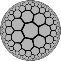
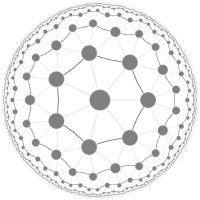
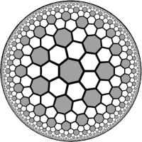
Figure 1: (a) order-3 heptagonal tiling, (b) the triangulation $G_{710}$, (c) truncated triangular tiling, (d) the triangulation $G_{711}$.

Figure 1 shows two tilings of the hyperbolic plane, the order-3 heptagonal tiling and its bitruncated variant, in the Poincaré disk model, together with their dual graphs, which we call $G_{710}$ and $G_{711}$. In the Poincaré model, the hyperbolic plane is represented as a disk. In the hyperbolic metric, all the triangles, heptagons and hexagons on each of these pictures are actually of the same size, and the points on the boundary of the disk are infinitely far from the center.

Recently, hyperbolic geometry has found application in the analysis of scale-free networks, which are ubiquitous in many fields, from network analysis to biology [23]. Fix a radial coordinate system in the hyperbolic plane ${\mathbb{H}}^{2}$, where every point is represented by two coordinates $(r,\phi)$, where $r$ is the distance from the fixed central point, and $\phi$ is the angle from the reference direction.

Definition 1.1.

The hyperbolic random graph model has four parameters: $n$ (number of vertices), $R$ (radius), $T$, and $\alpha$. Each vertex $v\in V(H)=\{1,\ldots,n\}$ is independently randomly assigned a point $\mu(v)=(r_{v},\phi_{v})$, where the distribution of $\phi_{v}$ is uniform in $[0,2\pi]$, and the density of the distribution of $r_{v}\in[0,R]$ is given by $f(r)={{\alpha\sinh(\alpha r)}\over{\cosh(\alpha R)-1}}$. Then, for each pair of vertices $v,w\in V(H)$, they are independently connected with probability $p(\delta(\mu(v),\mu(w)))$, where $\delta(x,y)$ is the distance between $x,y\in{\mathbb{H}}^{2}$, and $p(d)={1\over 1+e^{(d-R)/2T}}$.

It is known that, for correctly chosen values of $n$, $R$, $T$ and $\alpha$, the properties of hyperbolic random graph, such as its degree distribution or clustering coefficient, are similar to those of real world scale-free networks [12]. Perhaps the two most important algorithmic problems related to HRGs are sampling (generate a HRG) and MLE embedding: given a real world network $G$, map the vertices of $G$ to the hyperbolic plane in such a way that the edges are predicted as accurately as possible. The quality of this prediction is measured with log-likelihood, computed with the formula $\log L(\mu)=\sum_{v<w\in V(H)}\log p_{\{v,w\}\in E}(\delta(\mu(v),\mu(w)))$, where $p_{\phi}(d)=p(d)$ if $\phi$ is true and $1-p(d)$ if $\phi$ is false. These problems are non-trivial, as we have to sum over all pairs of vertices (thus an $O(n^{2})$ algorithm) just to compute the log-likelihood. The original paper [23] used an $O(n^{3})$ algorithm. Efficient algorithms have been found for generating HRGs in time $O(n)$ [4] and for MLE embedding real world scale-free networks into the hyperbolic plane in time ${\tilde{O}}(n)$ [3], which was a major improvement over previous algorithms [22, 25]. The algorithm in [3], which we call here the BFKL embedder, is based on an $O(n)$ method of approximating the log-likelihood.

Triangulations such as $G_{711}$ and $G_{710}$ from Figure 1 can be naturally interpreted as metric spaces, where the points are the vertices of the triangulations, and the distance $\delta(v,w)$ is the number of edges we have to traverse to reach $w$ from $v$. Such metric spaces have properties similar to the underlying hyperbolic plane; this similarity is much stronger than in the case of Euclidean triangulations. In particular, hyperbolic shapes such as straight lines, circles, equidistant curves or horocycles have their natural counterparts in the discrete world with very similar properties. This similarity can be defined more formally by saying that our triangulations are Gromov hyperbolic spaces [2]. A metric space is Gromov hyperbolic iff every geodesic triangle is $d$-slim, for some finite $d$. A geodesic from $u$ to $v$ is a path of length $\delta(u,v)$, and a geodesic triangle consists of a geodesic $g_{uv}$ from $u$ to $v$, $g_{vw}$ from $v$ to $w$, and $g_{wu}$ from $w$ to $u$. Such a triangle is $d$-slim iff every point on $g_{wu}$ lies in distance at most $d$ from $g_{uv}\cup g_{vw}$. Since for trees $d=0$, Gromov hyperbolicity (i.e., the value of $d$) can be seen as a measure of tree-likeness.

Our contribution. We propose a discrete analog of the HRG model, which we call the DHRG model: in our model, $\mu$ maps the nodes to the vertices of a triangulation, and the probability of two nodes $v_{1},\ v_{2}$ being connected depends on the graph distance between the vertices $\mu(v_{1})$ and $\mu(v_{2})$.

Such a discrete model lets us use a data structure we call the tally counter. The tally counter represents a set $S$ of vertices of a triangulation; we can add and remove vertices to it, and we can also answer queries of the form for the given vertex $w$, how many vertices in $S$ are in distance $d$ from $w$, where $d=0,\ldots,2R$?. This data structure lets us compute the log-likelihood of a DHRG embedding in $O(n+m)$ queries in a straightforward way, which is an important step in MLE embedders. Furthermore, it lets us to dynamically remap a vertex $v$ to another location and compute the log-likelihood of the new embeddding in $O(1+\deg(v))$ queries.

It is well known that many algorithmic problems can be easily solved on trees; it is also well known that many graph problems admit very efficient algorithms on graphs that are similar to trees, where similarity is most commonly measured using the notion of tree width [24]. For example, every fixed graph property definable in the monadic second order logic with quantification over sets of vertices and edges ($MSO_{2}$) can be checked in linear time on graphs of fixed tree width [8]. A similar thing happens in our case: tree-likeness of hyperbolic tesselations lets us to implement all the operations of the tally counter in $O(R^{2})$, while the distance between two vertices can be computed in $O(R)$. Since hyperbolic geometry exhibits exponential growth, $R$ is typically logarithmic in $n$.

Therefore, we can easily compute the log-likelihood of a DHRG embedding in time $O(nR^{2}+mR)$, where $n$ is the number of vertices and $m$ is the number of edges; this matches the complexity of the approximation method in the BFKL embedder [3] up to $R^{O(1)}$ factors. We believe this could be used to create an efficient MLE embedder, using discrete versions of the methods employed by that embedder; however, this is an area of further research. For now, we used the available implementation of the BFKL embedder to produce HRG embeddings, and transformed them to the DHRG model by moving every $\mu(v)$ to the nearest vertex of the triangulation. According to our experiments, despite the approximations introduced by our discretization, our method is much more accurate than the one used in the BFKL embedder, and it runs in comparable time. Another benefit of our method is its dynamic remapping property, which lets us improve the embeddings using a local search method: for every vertex $v$, try to move $\mu(v)$ to all its neighbors, and keep the change if it improves the log-likelihood. One iteration of such local search can be performed in time $O(nR^{2}+mR)$, and the local search stabilizes after a small number of iterations, which is a major improvement on the $O(n^{2})$ spring embedder implemented in the BFKL embedder. Our data structures also allow to generate DHRGs in time $O(nR^{2}+mR)$. While our algorithms match the best known algorithms up to $R^{O(1)}$ factors, we believe they have a significant advantage of simplicity: the algorithms for distance computation and the tally counter are straightforward, especially for theoretical computer scientists who have experience in discrete algorithmics and automata theory [19] rather than hyperbolic geometry. Furthermore, efficient local search might be useful on its own [5].

It is worth to note that the major breakthrough in [4] and [3] was achieved by using geometric structures based on partitioning hyperbolic disks into cells of the binary tiling. This is in some sense similar to our triangulations. However, we believe that avoiding the continuous representations altogether and working with more general hyperbolic tesselations than just the binary tiling makes our approach more elegant. Hyperbolic triangulations have many other applications, and they are beautiful and interesting in their own right. Exponential nature of the hyperbolic geometry makes many algorithmic problems challenging (for large values of $R$, it is impossible to keep the whole disk of radius $R$ in the memory) while it proves invaluable in the visualization of hierarchical data [15, 20]; mapping vertices of the visualized graph to distinct vertices of a regular triangulation allows for aesthetically pleasant representations of graphs [7]. Apart from visualizations, hyperbolic triangulations have been used to create more efficient self-organizing maps (HSOMs) [21]. They also arise naturally when working with bounded degree planar graphs; for example, many constructions in [9] are Gromov hyperbolic graphs. Hyperbolic geometry is useful in mathematical art and game design [14]. Our algorithms for computing distances in hyperbolic tesselations have found application in data vizualization [7] and in the implementation of HyperRogue [14], which we recommend as an intuitive introduction to hyperbolic tesselations and hyperbolic geometry in general.

While the $R^{O(1)}$ factors may be seen as a disadvantage, they are avoided in [23, 12, 3] by assuming that operations on floating point numbers are performed in time $O(1)$. However, any representation of the hyperbolic plane as a tuple of floating point numbers in a typical coordinate system is prone to precision errors. Indeed, the circumference of a hyperbolic circle of radius $r$ is $2\pi\sinh(r)=\Theta(e^{r})$. Therefore, if we are using $b$ bits for the angular coordinate, two points on the circle of radius $b\log(2)+\Theta(1)$ will be smashed into a single point, even if their exact distance is greater than 1. In our approach the vertices are represented instead as paths from the “root” vertex, thus avoiding such precision problems even for very large values of $R$. Even if we want to perform computations in the continuous hyperbolic plane, a “hybrid” approach where each point is represented by a vertex of our tesselation together with the coordinates relative to that vertex is useful to prevent precision errors. Such approach is used in HyperRogue [26].

Structure of the paper. In the next section we present the hyperbolic tesselations, and their properties which will be essential for our algorithms. Section 3 introduces our algorithms for calculating distances in the graph. In Section 4, we study how the distances in our graphs are related to the distances in the underlying hyperbolic plane. We define our DHRG model in Section 5, based on the intuitions from Section 4. We show how to apply our algorithms to work with DHRGs efficiently in Section 6. We have implemented [1] the log-likelihood computation and local search algorithms presented in Sections 3 and 5; Section 7 presents the experimental results on real world networks. We discuss possible directions for further work in Section 8. We also provide a browser-based interactive visualization of some concepts in this paper [1].

2 Hyperbolic triangulations

In a regular tesselation every face is a regular $p$-gon, and every vertex has degree $q$ (we assume $p,q\geq 3$). We say that such a tesselation has a Schläfli symbol $\{p,q\}$. Such a tesselation exists on the sphere iff $(p-2)(q-2)<4$, plane iff $(p-2)(q-2)=4$, and hyperbolic plane iff $(p-2)(q-2)>4$. In this paper we are most interested in triangulations ($p=3$) of the hyperbolic plane ($q>6$).

Contrary to the Euclidean tesselations, hyperbolic tesselations cannot be scaled: on a hyperbolic plane of curvature -1, every face in a $\{q,p\}$ tesselation, and equivalently the set of points closest to the given vertex in its dual $\{p,q\}$ tesselation, will have area $\pi(q\frac{p-2}{p}-2)$. Thus, among hyperbolic triangulations of the form $\{3,q\}$, $\{3,7\}$ is the finest, and they get coarser and coarser as $q$ increases.

For our applications it is useful to consider hyperbolic triangulations finer than $\{3,7\}$. Such triangulations can be obtained with the Golberg-Coxeter construction, which adds additional vertices of degree 6. Consider the $\{3,6\}$ triangulation of the plane, and take an equilateral triangle $X$ with one vertex in point $(0,0)$ and another vertex in the point obtained by moving $a$ steps in a straight line, turning 60 degrees right, and moving $b$ steps more. The triangulation $GC_{a,b}T$ is obtained from the triangulation $T$ by replacing each of its triangles with a copy of $X$ [1]. Regular triangulations are a special case where $a=1,b=0$. For short, we denote the triangulation $GC_{a,b}\{3,q\}$ with $G_{qab}$. Figure 1d shows the triangulation $G_{711}$.

Let $v_{0}$ be a vertex in a hyperbolic triangulation $G$ of the form $G_{qab}$. We denote the set of vertices of $G$ by $V(G)$. For $v,w\in V(G)$, let $\delta(v,w)$ be the length of the shortest path from $v$ to $w$. Below we list the properties of our triangulations which are the most important to us.

Proposition 2.1 (rings).

The set of vertices in distance $k$ from $v_{0}$ is a cycle.

We will call this cycle $k$-th ring, $R_{k}(G)$. We assume that all the rings $R_{k}(G)$ are oriented clockwise around $v_{0}$. Thus, the $i$-th successor of $v$, denoted $v+i$, is the vertex obtained by starting from $v$ and going $i$ vertices on the cycle. The $i$-th predecessor of $v$, denoted $v-i$, is obtained by going $i$ vertices backwards on the cycle. A segment is the set $S=\{v,v+1,\ldots,v+k\}\subsetneq R_{k}(G)$ for some $v\in V$ and $k\geq 0$; $v$ is called the leftmost element of $S$, and $v+k$ is called the rightmost element of $S$. By $[v,w]$ we denote the segment such that $v$ is its leftmost element, and $w$ is its rightmost element. For $v,w\in R_{k}(G)$, let $w-v$ be the smallest $i\geq 0$ such that $w=v+i$. We also denote $\delta_{0}(v)=\delta(v,v_{0})$. By $B_{k}(G)$ we denote the $k$-th ball (neighborhood of $v_{0}$), i.e., $B_{k}(G)=\bigcup_{i=0,\ldots,k}R_{k}(G)=\{v\in V|\delta(v,v_{0})\leq k\}$.

Proposition 2.2 (parents and children).

Every vertex (except the root $v_{0}$) has at most two parents and at least two children.

We use tree-like terminology for connecting the rings. A vertex $w$ is a parent of $v$ if there is an edge from $v$ to $w$ and $\delta_{0}(v)=\delta_{0}(w)+1$; in this case, $v$ is a child of $w$. Let $P(v)$ be the set of parents of $v\in R_{k}(G)$; it forms a segment of $R_{k-1}(G)$, and its leftmost and rightmost elements are respectively called the left parent $p_{L}(v)$ and the right parent $p_{R}(v)$. The set of children $C(v)$, leftmost child $c_{L}(v)$ and rightmost child $c_{R}(v)$ are defined analogously.

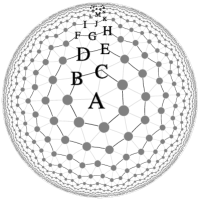
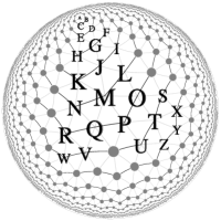
Figure 2: Triangulation $G_{711}$ with labeled vertices, in two perspectives.

Figure 2 depicts the triangulation $G_{711}$ with named vertices. Both pictures use the Poincaré disk model and show the same vertices, but the left picture is centered roughly at $v_{0}$ (labeled with $A$ in the picture), and the right picture is centered at a different location in the hyperbolic plane. Points drawn close to the boundary of the Poincaré disk are further away from each other than they appear – for example, vertices $T$ and $U$ appear very close in the left picture, yet in fact all the edges are roughly of the same length (in fact, there are two lengths – the distance between two vertices of degree 6 is slightly different than the distance between a vertex of degree 6 and a vertex of degree 7).

Vertices $X$, $Y$, and $Z$ are the children of $T$; its siblings are $S$ and $U$, and its parents are $O$ and $P$. The values of $P^{k}([Y])$ for consecutive values of $k$, i.e., the ancestor segments of $Y$, are: $[Y]$, $[T]$, $[O,P]$, $[L,M]$, $[I,K]$, $[F,H]$, $[D,E]$, $[B,C]$, $[A]$. Vertex $W$ has just a single ancestor on each level: $R$, $N$, $K$, $H$, $E$, $C$, $A$. Vertex $V$ has the following ancestor segments: $[Q,R]$, $[M,N]$, $[J,K]$, $[G,H]$, $[D,E]$, $[B,C]$, $[A]$. Note the tree-like nature of our graph: $[D,E]$ is the segment of ancestors for both $V$ and $Y$, and $[O,P]$ and $[Q,R]$ are already adjacent. This tree-like nature will be useful in the algorithms in Section 3.

Proposition 2.3 (canonical shortest paths).

Let $v,w\in V(G)$, and $\delta(v,w)=d$. Then at least one of the following is true:

• $v\in P^{d}(w)$,

• $w\in P^{d}(v)$,

• $p_{R}^{a}(v)+b=p_{L}^{c}(w)$, where $a+b+c=d$,

• $p_{R}^{a}(w)+b=p_{L}^{c}(v)$, where $a+b+c=d$.

In other words, the shortest path between any pair of two vertices $(v,w)$ can always be obtained by going some number of steps toward $v_{0}$, moving along the ring, and going back away from $v_{0}$. The cases where one of the vertices is an ancestor of the other one had to be listed separatedly because it is possible that $|P^{a}(v)|>2$ for $a>1$, thus $w$ might be neither the leftmost not the rightmost ancestor. Such a situation happens in $G_{711}$ for the pair of vertices labeled $(J,O)$ in Figure 2, even though $|P^{a}(v)|\leq 3$ always holds.

Proposition 2.4 (regular generation).

There exists a finite set of types $T$, a function $c:T\rightarrow T^{*}$, and an assignment $t:V(G)\rightarrow T$ of types to vertices, such that for each $v\in V(G)$, the sequence of types of all children of $v$ from left to right except the rightmost child is given by $c(t(v))$.

By $T^{*}$ we denote the set of finite words over an alphabet $T$. The rightmost child of $v$ is also the leftmost child of $v+1$, so we do not include its type in $c(t(v))$ to avoid redundancy. Our function $c:T\rightarrow T^{*}$ can be uniquely extended to a homomorphism $T^{*}\rightarrow T^{*}$, which we also denote with $c$, in the following way: $c(t_{1}\ldots t_{k})=c(t_{1})\ldots c(t_{k})$. By induction, the sequence of types of non-rightmost vertices in $C^{k}(v)$ is given by $c^{k}(t(v))$.

For regular triangulations $\{3,q\}$, the set of types is $T=\{0,1,2\}$, and the types correspond to the number of parents [1]. The root has type 0 and has $q$ children of type $1$, thus $c(0)=1^{q}$. For a vertex with $t=1,2$ parents, the leftmost child has type 2 (two parents), and other non-rightmost children all have type 1. Thus, we have $c(t)=21^{q-4-t}$. Such constructions for $\{3,q\}$ and $\{4,q\}$ grids have been previously studied by Margenstern [18, 17, 19].

For $GC_{1,1}$ triangulations there are 7 types, because we also need to specify the degree of vertex $v$ as well as the orientation (the degree of the first child). For Goldberg-Coxeter tesselations in general we need to identify the position of $v$ in the triangle $X$ used in the Goldberg-Coxeter construction.

Proposition 2.5 (exponential growth).

There exists a constant $\gamma(G)$ such that, for every vertex $v$, $|C^{k}(v)|=\Theta(\gamma(G)^{k})$.

Note that, if $c(t(v))=t_{1}\ldots t_{n}$, the number of non-rightmost vertices in $C^{k}(v)$ is given by $\sum_{i=1}^{n}|c^{k-1}(t_{i})|$. This gives a linear recursive system of formulas for computing $|C^{k}(v)|$; $\gamma$ is the largest eigenvalue of the respective matrix. We have $\gamma\approx 2.6180339$ for $G_{710}$ and $\gamma\approx 1.72208$ for $G_{711}$.

Proposition 2.6 (Gromov hyperbolicity).

There exists a constant $D(G)$ such that, for every $d>D(G)$ and $x\in V(G)$, the distance from $x$ to $x+d$ is smaller than $d$.

This property gives an upper bound on the value of $b$ in Proposition 2.3, and thus it will be crucial in our algorithms computing distances between vertices of $G$. We call this property Gromov hyperbolicity, because its combination with Proposition 2.3 says that the triangle with vertices in $v_{0}$, $v$ and $w$ is slim. Euclidean triangulations do not have this property.

Given the canonicity of shortest paths and regular generation, the value of $D(G)$ can be found with a simple algorithm. We have verified experimentally for $a,b\leq 8$ that $D(G_{qab})=2a+b$.

Definition 2.7.

A regularly generated hyperbolic triangulation (RGHT) is a triangulation which satisfies all the properties listed above.

The properties above hold not only for the triangulations of the form $G_{qab}$. Probably the simplest, though geometrically less regular, example of a RGHT is obtained by taking a full infinite binary tree, and additionally connecting each vertex to its cyclic left and right sibling, and additionally the right child of its left sibling. Such tiling has just one type $\star$, and $c(\star)=\star\star$. This could be seen as a variant of the binary tiling of the hyperbolic plane. Our algorithms will work with such tilings [1].

There are triangulations where the properties above do not hold; this happens even for face-transitive (Catalan) triangulations. For example, the triangulation with face configuration V5.8.8 [1] has vertices with three parents; this causes the tree-like distance property to fail (consider a vertex $v$ with 3 parents and the shortest path from the leftmost parent of $v$ to $v+1$). If we split every face of $\{3,7\}$ into three isosceles triangles, we obtain the triangulation with face configuration V14.14.3 [1], where the sets $R_{k}(G)$ are no longer cycles (vertices repeat on them), causing the regular generation to fail. More sophisticated but qualitatively similar variants of our algorithms work for tesselations described above; we expect this to hold for any Gromov hyperbolic triangulations. We concentrate on the regularly generated case in this paper, because non-regularly generated triangulations are much less useful for all our applications: they are much less uniform because of the high variance of degrees and edge lengths.

We can also consider square tilings, i.e., $GC_{a,b}\{4,q\}$ for $q\geq 5$ (Goldberg-Coxeter construction for square tilings is defined analogously) [1]. The major difference here is that the rings $R_{k}(G)$ are disconnected rather than cycles. However, this only makes our algorithms simpler: the canonical shortest paths (Proposition 2.3) no longer have to go across the ring, i.e., $b$ always equals 0. However, despite the greater simplicity and better performance, square tilings give worse results for the HRG embedding applications. This is not surprising, as they provide a less accurate approximation of hyperbolic distance.

Our ring structure has a singularity in $v_{0}$. It is possible to avoid this singularity by changing our construction a bit, by making $R_{d}(G)$ into infinite paths (horocycles) [1]. Another possible change to our construction is to connect the last element of $R_{d}(G)$ with the adjacent element of $R_{d+1}(G)$, thus putting all the vertices of $G$ in a single spiral [9].

3 Computing distances in hyperbolic triangulations

It is not feasible to represent all vertices in, say, $B_{100}(G_{711})$ in computer memory – there are more than $10^{23}$ of them! However, Proposition 2.4 lets us generate the vertices in our RGHT lazily. That is, represent our vertices with pointers, start from the root, and generate other vertices when asked for them. In particular, each vertex $v$ is represented with a pointer to a structure which contains $\delta_{0}(v)$, the type of $v$, the pointers to $p_{L}(v)$, $p_{R}(v)$, $v-1,$ $v+1,$ $c_{L}(v),$ and the index of $v$ among the children of $p_{R}(v)$; the last three pointers are NULL if the given neighbor has not yet been computed. Such a structure allows us to compute all the neighbors of the given vertex in amortized time $O(1)$ for a fixed triangulation. In this section we show how to compute distances in a RGHT, based on this data structure.

Theorem 3.1.

Fix a RGHT $G$. Then $\delta(v,w)$ can be computed for $v,w\in G$ in time $O(\delta(v,w))$.

Proof (sketch).

The idea of the algorithm is to find the shortest path given in Proposition 2.3 and limited according to Proposition 2.6. Suppose that $\delta_{0}(v)=d^{\prime}+\delta_{0}(w)$, where $d^{\prime}\geq 0$. For each $i$ starting from 0 we compute the endpoints of the segments $P^{d^{\prime}+i}(v)$ and $P^{i}(w)$. We check whether these segments are in distance at most $D(G)$ on the ring; if no, then we can surely tell that we need to check the next $i$; if yes, we know that the shortest path can be found on one of the levels from $i$ to $i+\lfloor D(G)/2\rfloor$. We compute the length of all such paths and return the minimum. The full algorithm and the proof of its correctness is given in the Appendix A. ∎

It is worth to note that $D(G_{k11})=3$ and $D(G_{k10})=2$; these RGHTs are most appropriate for our applications, and our algorithm is very efficient for them. With some preprocessing, we can optimize to $O(\log\delta(v,w))$ per query – precompute $p_{L}^{a}(v)$ for each $v\in V$ and $a$ that is a power of two.

A distance tally counter for a graph $G=(V,E)$ represents a modifiable function $f:V\rightarrow{\mathbb{R}}$ with the following operations:

• Initialize: $f$ is initialized with the constant 0 function

• Add($v$, $k$): add $k$ to $f(v)$

• Tally($v$): return an array $A$ such that, for every $d\in{\mathbb{N}}$, $A[d]=\sum_{w\in V:\delta(v,w)=d}f(w)$ (if $d$ is out of bounds of $A$, we assume that $A[d]=0$)

Theorem 3.2.

Fix a RGHT $G$. A distance tally counter can be implemented working in memory $O(\sum_{w\in W:f(w)\neq 0}\delta_{0}(w)^{2})$, initialization in time $O(1)$, and Add($v$) and Tally($v$) in time $O(\delta_{0}(v)^{2})$.

Proof (sketch).

A segment is good if it is of the form $P^{d}([v,v])$ for some $v\in V$ and $d\in{\mathbb{N}}$. Note that the algorithm from the proof of Theorem 3.1 can be seen as follows: we start with two segments $[v,v]$ and $[w,w]$, and then apply the operation $P$ to each of them until we obtain good segments which are close. Our algorithm will optimize this by representing all the good segments coming from vertices $v$ added to our structure.

We call a vertex or good segment is called active if it has been already generated, and thus is represented as an object in memory. For each active vertex $v\in V$ we keep two lists $L_{L}(v),L_{R}(v)$ of active segments $S$ such that $v$ is respectively the leftmost and rightmost element of $S$. Each active segment $S$ also has a pointer to $P(S)$, which is also active (and thus, all the ancestors of $S$ are active too), and a dynamic array of integers $a(S)$. Initially, there are no active vertices or good segments; when we activate a segment $S$, its $a(S)$ is initially filled with zeros.

The operation Add($v$, $k$) activates $v$, and $S=[v,v]$ together with all its ancestors. Then, for each $i=0,\ldots,\delta_{0}(v)$, it adds $k$ to $a(P^{i}(S))[i]$.

The operation Tally($w$) activates $w$ and $S=[w,w]$ together with all its ancestors. We return the vector $A$ obtained as follows. We look at $p^{i}(S)$ for $i=0,\ldots,\delta_{0}(v)$, and for each $p^{i}(S)$, we look at close good segments $q^{\prime}$ on the same level, baswed on the lists $L_{L}(w),L_{r}(w)$ for all $w$ in distance at most $D(G)$ from $p_{i}(S)$. The intuition here is as follows: the algorithm from Theorem 3.1, on reaching $p^{i_{1}}(v)=S$ and $p^{i_{2}}(w)=S^{\prime}$, would find out that these two pairs are close enough and return $i_{1}+i_{2}+\delta(S,S^{\prime})$; in our case, for each $c$ such that $a(S^{\prime})[c]\neq 0$, we will instead add $a(S^{\prime})[c]$ to $A[a_{1}+\delta(S,S^{\prime})+c]$. We have to make sure that we do not count vertices which have been already counted. ∎

4 Graph distances versus hyperbolic distances

Let $j:V(G)\rightarrow{\mathbb{H}}^{2}$ be the function mapping the vertices of our triangulation to their position on the hyperbolic plane. $j(v)$ can be computed by applying $d=\delta_{0}(v)$ isometries to $j(v_{0})$, with $i$-th isometry depending only on the type of $p_{R}^{d-i+1}(v)$ and the index of $p_{R}^{d-i}(v)$ among its children.

Intuition 4.1.

For $v,w\in V(G)$, let $d=\delta(v,w)$, and $r=\delta(j(v),j(w))$. Then $d$ and $r$ are approximately proportional.

Stating and proving this intuition formally appears to be challenging, as we have to deal both with the discrete structure of the triangulation, and the continuous hyperbolic geometry. From the regularity of our tesselation we get that $d=\Theta(r)$; we cannot give a better estimate (e.g., $d=\alpha r+\Theta(1)$) because the density of rings depends on the direction. However, we can guess that, on average, $r\approx d\log\gamma$. This is because, in the hyperbolic plane, the area and circumference of a circle of radius $r$ given in absolute units is given by $\cosh(r)-1$ and $\sinh(r)$ respectively, which are $\Theta(e^{r})$; from Proposition 2.5 we know that this corresponds to $\Theta(\gamma^{d})$ vertices of our graph, yielding $r\approx d\log\gamma$ after taking the logarithm of both sides.

We can also expect the grid approximation to be better than the corresponding Euclidean one. Consider the regular triangulation $G_{610}$ on the Euclidean plane, in the standard embedding where every edge has length 1. Let $v=v_{0}$ and $W$ be a random vertex in $R_{d}(G_{610})$. From basic geometry we obtain that $r\in[\frac{\sqrt{3}}{2}d,d]$. The standard deviation of $r$ will be linear in $d$, because the ratio $r/d$ depends on the angle between the line $(v_{0},W)$ and the grid lines. However, in the hyperbolic plane, because of the exponential expansion, this angle constantly changes as the line $(v_{0},W)$ traverses the grid, leading to the following conjecture:

Conjecture 4.2.

Let $G=G_{qab}$, and $W\in R_{d}(G)$ be randomly chosen. Then $\delta(j(v_{0}),j(W))=c_{1}d+c_{0}+X$, where $EX=o(1)$, $\mbox{Var}\ X=\Theta(d)$.

The results of experimental verification agree with the conjecture for $G_{711}$, $G_{710}$ and $G_{810}$, although $c_{1}$ is slightly larger than $\log\gamma$ in these cases. While Conjecture 4.2 remains unproven, it is worth to remind that it is not essential to our work – our triangulations interpreted as abstract metric spaces exhibit hyperbolic properties in their own right.

5 Discrete hyperbolic random graphs

In this section we use our intuitions from the previous section to define the discrete hyperbolic random graph model (DHRG), the discrete version of the HRG model (Definition 1.1).

In our model, we map vertices $v\in V(H)$ not to points in the continuous hyperbolic plane, but to the vertices of our RGHT $G$, i.e., $\mu:V(H)\rightarrow V(G)$. The density function $f(r)$ from the HRG model cannot be reproduced exactly, but we can use $f(r)={\alpha e^{\alpha r}}/(e^{\alpha r}-1)$, which is a very good approximation (it only slightly changes the low probability of placing a vertex very close to the center).

Definition 5.1.

A discrete hyperbolic random graph (DHRG) over the RGHT $G$ with parameters $n,$ $R,$ $T,$ and $\alpha$ is a random graph $H=(V(H),E(H))$ constructed as follows:

• The set of vertices is $V(H)=\{1,\ldots,n\}$,

• Every vertex $v\in V(H)$ is independently randomly assigned a vertex $\mu(v)\in B_{R}(G)$ in such a way that the probability that $\mu(v)=w$ is proportional to $\frac{e^{d\alpha}}{|R_{d}(G)|}$, where $d=\delta_{0}(w)$;

• Every pair of vertices $v_{1},v_{2}\in V(H)$ are independently connected with an edge with probability $p(\delta(\mu(v_{1}),\mu(v_{2})))$, where $p(d)={1\over 1+e^{(d-R)/2T}}$.

Note that the definition permits $\mu(v_{1})=\mu(v_{2})$ for two different vertices $v_{1},v_{2}\in V(H)$ – this is not a problem, furthermore, such vertices $v_{1}$ and $v_{2}$ are not necessarily connected, nor do they need to have equal sets of neighbors.

DHRG mappings can be converted to HRG by composing $\mu$ with $j$, and the other conversion can be done by finding the nearest tesselation vertex to $\mu(v)$ for each $v\in V(G)$. From Conjecture 4.2 we expect the DHRG parameters $\alpha$, $R$, and $T$ to be related to the HRG parameters by the factor of $\log\gamma$.

Theorem 5.2.

DHRG with parameters $\alpha>\log\gamma/2$, $R$, $T$ and $n$ has a power law degree distribution with exponent $\beta=1+2(\alpha/\log\gamma)$. Furthermore, the expected clustering coefficient, average degree, and approximate degree distribution of a DHRG with given parameters can be computed in time polynomial in $R$. (Proof in the Appendix.)

6 Algorithms for DHRG

We show how the algorithms from Section 3 allow us to deal with the DHRG model efficiently.

Computing the likelihood. Computing the log-likelihood in the continuous model is difficult, because we need to compute the sum over $O(n^{2})$ pairs; a better algorithm was crucial for efficient embedding of large real world scale-free networks [3]. The algorithms from the previous section allow us to compute it quite easily in the DHRG model. To compute the log-likelihood of our embedding of a network $H$ with $n$ vertices and $m$ edges, such that $\delta_{0}(v)\leq R$ for each $v\in V(H)$, we:

• for each $d$, compute $\textsc{Tally}[d]$, which is the number of pairs $(v,w)$ such that $\delta(v,w)=d$ – the distance tally counter allows doing this in a straightforward way (simply by doing Add($\mu(v)$, 1) for each $v\in V(H)$), in time $O(nR^{2})$.

• for each $d$, compute $\textsc{Edgetally}[d]$, which is the number of pairs $(v,w)$ connected by an edge such that $\delta(v,w)=d$ – this can be done in time $O(mR)$ simply by using the distance algorithm for each of $m$ edges.

After computing these two values for each $d$, computing the log-likelihood is straightforward. One of the advantages over [3] is that we can then easily compute the log-likelihood obtained from other values of $R$ and $T$, or from a function $p(d)$ which is not necessarily logistic.

Improving the embedding. A continuous embedding can be improved by a spring embedder [13]. Imagine that there are attractive forces between connected pairs of vertices, and repulsive forces between unconnected pairs. The embedding $m$ will change in time as the forces push the vertices towards locations in such a way that the quality of the embedding, measured by log-likelihood, is improved. However, computationally, spring embedders are very expensive – there are $O(n^{2})$ forces, and potentially, many steps of our simulation could be necessary.

On the other hand, our algorithms allow to improve DHRG embeddings quite easily. We use a local search algorithm. Suppose we have computed the log-likelihood, and on the way we have computed the vectors Tally and Edgetally, as well as the distance tally counter where every $\mu(v)$ has been added. Now, let $v^{\prime}\in V(H)$ be a vertex of our embedding, and $w\in V(G)$. Let $\mu^{\prime}$ be the new embedding given by $\mu^{\prime}(v^{\prime})=w$ and $\mu^{\prime}(v)=\mu(v)$ for $v\neq v^{\prime}$. Our auxiliary data allows us then to compute the log-likelihood of $\mu^{\prime}$ in time $O(R^{2}+R\deg(w))$.

This allows us to try to improve the embedding in the following way: in each step, for each $v\in V(G)$, consider all neighbors of $\mu(v)$, compute the log-likelihood for all of them, and if for some $\mu^{\prime}$ we have $\log L(\mu^{\prime})>\log L(\mu)$, replace $\mu$ with $\mu^{\prime}$. Assuming the bounded degree of $G$, this can be done in time $O(R^{2}n+Rm)$.

Generating a random graph. Generating large HRGs is not trivial – a naive algorithm works in $\Theta(n^{2})$; algorithms working in $O((n^{3/2}+m)\log n)$ and $O(n)$ [25, 4] are known. Our algorithms allow to generate DHRGs quite easily in $O(nR^{2}+mR)$.

The first step is to generate the vertices. For each vertex $v=\{1,\ldots,n\}$, we choose $d=\delta_{0}(v)$ (according to the given distribution), and then we have to randomly choose $v$ from the $|R_{d}(v)|$ possibilities. This can be done iteratively: we create a sequence of vertices $v_{0}$, …, $v_{d}$, where $v_{0}$ is the root, and $v_{k+1}$ is a non-rightmost child of $v_{k}$. The probability of choosing the particular $v$ as $v_{k}$ should be proportional to $a_{d-k}(v)$, where $a_{i}(v)=|C^{d-k}(v)|-1=|c^{d-k}(t(v))|$ can be obtained by matrix multiplication ($O(R)$ preprocessing).

The second step is to generate the edges. This can be done by modifying the algorithm computing the vector $\textsc{Tally}[d]$ – when we add $k$ to $\textsc{Tally}[d]$, we now also add each of the edges with the probability $p(d)$. Thus, we need to choose a subset of $S=\{1,\ldots,k\}$ where each element is independently chosen with probability $p$. $\min S$ has a geometric distribution Geo($p$), except the cases where $S=\emptyset$ which are represented by Geo($p$)¿$k$; assuming that Geo($p$) can be sampled in $O(1)$, this allows us to generate $\min S$ in time $O(1)$, and the rest of $S$ can then be generated in the same way. Then, trace the elements of $S$ back to their original vertices, which can be done in $O(R)$ per edge by following the tree of active segments back. The whole algorithm works in time $O(nR^{2}+mR)$, where $n$ is the number of vertices and $m$ is the number of generated edges.

7 Experimental results

We have implemented the log-likelihood and local search algorithms outlined in the previous section, and conducted experiments on real world network data. More details are in the Appendix, and the results are included with our implementation [1].

Facebook social circle network. First, we test our model on a relatively small network. We have chosen the Facebook social circle network, coming from the SNAP database [16] and included with the hyperbolic embedder implementing the algorithm by Bläsius et al [3], which we will refer to as BFKL. This network has $N=4039$ nodes and $M=88234$ edges. BFKL has mapped this graph to the hyperbolic plane, using parameters $R=12.576$, $\alpha=0.755$, $T=0.1$. We have computed the log-likelihood as $L_{1}=-516534$. This looks extremely bad at first, as it is worse than the log-likelihood of the trivial model where each edge exists with probability $M/{N\choose 2}$, which is $L_{0}=-487133$; however, this is because the influence of the parameter $T$ on the quality of the embedding is small [22], and thus BFKL uses a small value of $T=0.1$, which does not necessarily correspond to the network. The best log-likelihood of $L_{2}=-176132$ is obtained for $R_{2}=11.09358$ and $T_{2}=0.54336$.

Now, we convert this embedding into the DHRG model, by finding the nearest vertex of $G_{711}$ for each $v\in V(H)$. The best log-likelihood $L_{3}=-179125$ is obtained for $R_{3}=20.39395$ and $T_{3}=1.01295$; as predicted in Section 5, $T_{2}/T_{3}\approx R_{2}/R_{3}\approx\log\gamma$. Our log-likelihood $L_{3}$ is slightly worse than $L_{2}$, but this is not surprising – first, our edge predictor has lost some precision in the input because of the discrete nature of our tesselation, and second, the original prediction was based on the hyperbolic distance $r$ while our prediction is based on the tesselation distance $d$, and the ratio of $r$ and $d$ depends on the direction. We also compute the log-likelihood obtained by a model where the edge probability is $p(d)=\textsc{Edgetally}[d]/\textsc{Tally}[d]$, which corresponds to using the best possible function $p(d)$ (not necessarily logistic); we obtain $L_{4}=-177033$, which is only slightly better than $L_{3}$. This shows that the logistic function is close to the optimum.

Now, we try our local search algorithm. The points stopped moving in the $k$-th iteration, for $k=22$. This allows us to improve the log-likelihood of $L_{5}=-167991$, again for the best values of $R_{5}=20.710576$ and $T_{5}=0.964954$, and the optimal log-likelihood to $L_{6}=-165338$.

Now, we convert our mapping back to the HRG model, obtaining the log-likelihood of $L_{7}=-168445$ for the optimal values of $R_{7}=11.17756$ and $T_{7}=0.52578$. Note that $L_{7}$ is significantly better than $L_{2}$; hence, despite converting from HRG to DHRG and back, our method was successful at finding a better continuous embedding.

The running time of parts of our algorithm were: $t_{1}$=0.4 s (converting), $t_{2}$=0.067 s (computing Edgetally), $t_{3}$=0.031 s (computing Tally), $t_{4}$=40 s (local search). The BFKL embedder computes the log-likelihood in 0.3 seconds, which is comparable. However, their spring embedder working in quadratic time is much slower than our local search.

The respective values obtained on $G_{710}$ were: $t_{1}=0.5s$, $t_{2}=34ms$, $t_{3}=19ms$, $k=29$, $t_{4}=22s$, $L_{3}=-182721$, $L_{4}=-188134$, $L_{5}=-170074$, $L_{6}=-168006$, $L_{7}=-170886$. $G_{710}$ is coarser than $G_{711}$, hence it is not surprising that its results are slightly worse; also the smaller size and greater simplicity of $G_{710}$ improves the running time. Yet, the general qualitative effects are similar. Using finer triangulations such as $G_{753}$ yields minor improvements in the resulting log-likelihood at the cost of significant performance downgrade, due to the increase in the values of $R$ and $D(G)$.

GitHub following graph. To benchmark our algorithm on a large network, we study the embedding of a social network observed in GitHub repository hosting service. In GitHub convention, following means that a registered user agreed to be sent notifications about other user’s activity within the service. This relationship can be represented by the means of the graph of following $\mathcal{G}_{f}$. There is an edge in $\mathcal{G}_{f}$ between A and B iff A follows B. Decision about following a particular user can be simultaneously driven by their popularity within the network and the similarity to the interested user, which suggests hyperbolic geometry can be intrinsic in the development of $\mathcal{G}_{f}$. $\mathcal{G}_{f}$ was also proved to show power-law-like scale behavior [6], that is why we believe it is a sound benchmark for our analysis. Since the complete download of GitHub data is impossible, our dataset is combined from two sources: GHTorrent project [10] and GitHubArchive project [11]. The analyzed network contains information about the following relationships that occurred in the service from 2008 to 2009.

The graph has $n$=74946 vertices and $m$=537952 edges (since we are working with an undirected graph, an edge appears between A and B if either A follows B or B follows A). The BFKL embedder has chosen parameters $R=20.9037$ and $\alpha=0.855$, and computes the log-likelihood in 5 seconds. The results for $G_{710}$ are as follows: $t_{1}=12$ s, $t_{2}=2$ s, $t_{3}=0.5s$, $L_{0}=-4364526$, $L_{3}=-3976515$, $T_{3}=1.398666$, $R_{3}=9.063012$, $L_{4}=-3859688$. After 6 iterations of local search (25s each) the results have been improved to $L_{5}=-3571941$, $L_{6}=-3542740$; after 100 iterations the results are only slightly better, at -3545664 and -3527397. The time $t_{2}+t_{3}$ is still comparable to BFKL. Using an even coarser $G_{810}$ reduces the running time per iteration by about $\frac{1}{4}$, without a significant reduction in quality.

8 Conclusion

We have shown efficient algorithms for computing the distances between points in regularly generated hyperbolic triangulations, and distances between a given point and a set of points. We have shown how to apply these algorithms to work with the DHRG model efficiently, and how our DHRG model can be used to improve the results of the BFKL embedder. Creating a DHRG embedder is an direction of further research; we believe that the ideas underlying the BFKL embedder could be applied to the DHRG case. It is also interesting to what extent our algorithms for RGHTs can be generalized to wider classes of hyperbolic graphs, such as graphs with Gromov hyperbolicity $\delta$ [2].

We are very grateful to the anonymous referees for their careful reading of an earlier version of this work. Many parts of the paper have been greatly improved as a result of their insightful and constructive comments.

Appendix A Omitted proofs

1. function distance$(v_{1},v_{2})$:

2. for $i\in\{1,2\}$:

3. $l_{i}:=v_{i}$

4. $r_{i}:=v_{i}$

5. $d_{i}:=\delta_{0}(v_{i})$

6. $a_{i}:=0$

7. function push($i$):

8. $a_{i}:=a_{i}+1$

9. $d_{i}:=d_{i}-1$

10. $l_{i}:=p_{L}(l_{i})$

11. $r_{i}:=p_{R}(r_{i})$

12. while $d_{1}>d_{2}:$

13. push(1)

14. while $d_{2}>d_{1}:$

15. push(2)

16. for $i\in\{1,2\}$ if $v_{i}\in[l_{i},r_{i}]:$

17. return $a_{3-i}$

18. $d:=\infty$

19. while $a_{1}+a_{2}<d$:

20. for $i\in\{1,2\}$ for $k\in\{0,\ldots,t_{2}\}$ if $l_{i}=r_{3-i}+k:$

21. $d:=\min(d,a_{1}+a_{2}+k)$

22. push(1)

23. push(2)

24. return $d$

Figure 3: Pseudocode of the algorithm from Theorem 3.1.

Proof of Proposition 2.3.

Let $v,w\in V(G)$ for a triangulation $G$ satisfying the previous properties. Let $(v=v_{0},v_{1},v_{2},\ldots,v_{d}=w)$ be a path from $v_{0}=v$ to $v_{d}=w$ of length $d$. We will show that a path from $v$ to $w$ exists which is of the form given in Proposition 2.3 and is not longer than $d$.

In case if $v\in P^{d}(w)$ or $w\in P^{d}(v)$, the hypothesis trivially holds, so assume this is not the case.

Each edge from ${v_{i}}$ to ${v_{i+1}}$ on the path is one of the following types: right parent, left parent, right sibling, left sibling, right child (inverse of left parent, i.e., any non-leftmost child), left child (inverse of right parent, i.e., any non-rightmost child). We denote the cases as respectively ${v_{i}}\stackrel{{\scriptstyle RP}}{{\rightarrow}}{v_{i+1}}$, ${v_{i}}\stackrel{{\scriptstyle LP}}{{\rightarrow}}{v_{i+1}}$, ${v_{i}}\stackrel{{\scriptstyle RS}}{{\rightarrow}}{v_{i+1}}$, ${v_{i}}\stackrel{{\scriptstyle LS}}{{\rightarrow}}{v_{i+1}}$, ${v_{i}}\stackrel{{\scriptstyle RC}}{{\rightarrow}}{v_{i+1}}$, ${v_{i}}\stackrel{{\scriptstyle LC}}{{\rightarrow}}{v_{i+1}}$. We use the symbols $x,y$ if we do not care about the sides.

If ${v_{i}}\stackrel{{\scriptstyle xC}}{{\rightarrow}}{v_{i+1}}\stackrel{{\scriptstyle yP}}{{\rightarrow}}{v_{i+2}}$, then we can make the path shorter (${v_{i}}$ and ${v_{i+2}}$ are both children of ${v_{i+1}}$ and thus they must be the same or adjacent).

If ${v_{i}}\stackrel{{\scriptstyle xS}}{{\rightarrow}}{v_{i+1}}\stackrel{{\scriptstyle yP}}{{\rightarrow}}{v_{i+2}}$, then let $u$ be such that ${v_{i}}\stackrel{{\scriptstyle yP}}{{\rightarrow}}u$. Either $u={v_{i+2}}$ or $u$ is adjacent to ${v_{i+2}}$, so we can replace this situation with ${v_{i}}\stackrel{{\scriptstyle yP}}{{\rightarrow}}{v_{i+2}}$ or ${v_{i}}\stackrel{{\scriptstyle yP}}{{\rightarrow}}u\stackrel{{\scriptstyle zS}}{{\rightarrow}}{v_{i+2}}$, without making the path longer. The case ${v_{i}}\stackrel{{\scriptstyle yC}}{{\rightarrow}}{v_{i+1}}\stackrel{{\scriptstyle xS}}{{\rightarrow}}{v_{i+2}}$ is symmetric.

Therefore, all the $xP$ edges must be before all the $xS$ edges, which must be before all the $xC$ edges. Furthermore, clearly all the $xS$ edges must go in the same direction – two adjacent edges moving in opposite directions cancel each other.

We will now show that all the edges have to go in the same direction (right or left). This direction will be called $m\in\{L,R\}$. There are three cases:

• there are $xS$ edges – if they do not all go in the same direction, then two adjacent ones moving in the opposite directions cancel each other, so we can get a shorter path by removing them. Otherwise, let $m$ be the common direction.

• there are no $xS$ edges, and the vertex between $xP$ edges and $xC$ edges is the root – in this case, we get from $v$ to the root using $a$ parent edges, and then from the root to $w$ using $c$ child edges. If we replace the first $a$ edges with right parent edges, we still get to $v_{0}$; symmetrically, we replace the last $c$ edges with right child edges.

• there are no $xS$ edges, and the vertex between $xP$ edges and $xC$ edges is $v_{i}$ which is not the root – then, the main direction is $R$ iff $v_{i-1}$ is to the left from $v_{i+1}$ among the children of $v_{i}$, and $L$ otherwise.

Now, we can assume that all the edges in the $xC$ go in the same direction (i.e., they are $mC$ edges). Indeed, if this is not the case, let $m^{\prime}$ be the opposite of $m$, and take the last $m^{\prime}C$ edge: ${v_{i}}\stackrel{{\scriptstyle m^{\prime}C}}{{\rightarrow}}{v_{i+1}}\stackrel{{\scriptstyle m?}}{{\rightarrow}}{v_{i+2}}$. In all cases, let $u$ be such that ${v_{i}}\stackrel{{\scriptstyle mC}}{{\rightarrow}}u$. By case by case analysis, we get that ${v_{i}}\rightarrow u\rightarrow{v_{i+2}}$ the path is either shorter (i.e., $u={v_{i+2}}$) or pushes the $m^{\prime}C$ edge further the path. Ultimately, we get no $m^{\prime}C$ edges in the $xC$ part. By symmetry, we also have no $m^{\prime}P$ edges in the $mP$ part.

Therefore, our path consists of $a$ $mC$ edges, followed by $b$ $mS$ edges, followed by $c$ $mP$ edges. This corresponds to the last two cases of Proposition 2.3 (depending on whether $m$ is $R$ or $L$), therefore proving it. ∎

Proof of Proposition 2.6.

We will show how to compute $D(G)$ algorithmically based on the previous properties. We initialize the lower bound on $D(G)$ to 0, and call the function find_sibling_limit($v_{1}$, $v_{2}$) for every pair of vertices in $R_{1}(G)$. That function compute $v_{2}-v_{1}$, and check whether it is smaller than the length of a path which goes through lower rings; if yes, we update our lower bound on $D(G)$. Then, find_sibling_limit calls itself recursively for every $(w_{1},w_{2})$ where $w_{1}$ which is non-rightmost child of $v_{1}$ and every $w_{2}$ which is non-rightmost child of $v_{2}$.

This ensures that every pair of vertices is checked. Of course, this is infinitely many pairs. However, recursive descent is not necessary if:

• there is a vertex in the segment $[v_{1}+1,v_{2}-1]$ which produces an extra child in every generation.

• another pair $(v_{1},v_{2})$ previously considered had the same sequence of types of vertices in $[v_{1},v_{2}]$, and the same distances from $v_{1}$ to $v_{2}-1$ and from $v_{1}$ to $v_{2}$ (the results for any pairs of the descendants of the current pair would be the same as the results for the respective pairs of descendants of the earlier pair).

This algorithm is implemented in regular.cpp [1]. Proposition 2.6 can be verified for the given triangulation by running this algorithm or by manual case-by-case analysis. ∎

Proof of Theorem 3.1.

The pseudocode of our algorithm is given in Figure 3. It uses five integer variables $a_{i},d_{i},d$ and four vertex variables $l_{i}$, $r_{i}$ ($i=1,2$). Variables $a_{i}$, $d_{i}$, $l_{i}$ and $r_{i}$ are modified only by the function push($i$), which lets us keep the following invariant: $\delta_{0}(l_{i})=\delta_{0}(r_{i})=d_{i}$, $l_{i}=p_{L}^{a_{i}}(v_{i})$, $r_{i}=p_{R}^{a_{i}}(v_{i})$.

The lines (16-17) deal with the first two cases of the Proposition 2.3.

The main loop in lines (19-23) deals with the last two cases. At all times $d$ is the currently found upper bound on $\delta(v,w)$. It is easy to check that the specific shortest path given in Proposition 2.3 will be found by our algorithm.

Every iteration of every loop increases $a_{1}$ or $a_{2}$, and an iteration can occur only if $a_{1}+a_{2}<\delta(v,w)$. Therefore, the algorithm runs in time $O(\delta(v,w))$. An implementation is available (see Appendix B, file segment.cpp). ∎

Proof of Theorem 3.2.

We have not written down the pseudocode nor the proof, but an implementation is available (see Appendix B, file segment.cpp). ∎

Proof of Theorem 5.2.

Power law.

Take a DHRG $V$ with parameters $N$, $\alpha$, $R$, and $T$. Let $X$ be the degree of a random vertex of $V$. We have to show that $P(X>x)=\Theta(x^{-\beta+1})$.

A random vertex will be in ring $j$ with probability $\Theta(c^{R-j})$, where $c=e^{-\alpha}<1$.

Let $\gamma$ be the growth constant of our RGHT $G$. Take two random points $v_{1}$, $v_{2}$ from $R_{d}(G)$. What is the distance between $v_{1}$ and $v_{2}$?

Let $l$ be the distance between $v_{1}$ and $v_{2}$ along the cycle, i.e., $v_{1}+l=v_{2}$. From regularity, the distance between $P^{k}(x_{1})$ and $P^{k}(x_{2})$ is then $l/\gamma^{k}+O(1)$. Thus, the algorithm from Theorem 3.1 will stop after $s=\log_{\gamma}(l)+O(1)$ steps, and return $2s+O(1)$.

We could view this as follows: the distance between two random points from $R_{d}(G)$ is $2d-2\min(B,d)+O(1)$, where $B$ has geometric distribution with parameter $1/\gamma$; intuitively, $B$ corresponds to the length of the common branch of the pathes from $v_{0}$ to $v_{1}$ and $v_{2}$. This formula extends to random points from different rings: $d(d_{1},d_{2},B)=d_{1}+d_{2}-2\min(B,d_{1},d_{2})+O(1)$.

Now, take a DHRG with parameters $N$, $\alpha$, $R$, and $T$. A random vertex will be in ring $j$ with probability $\Theta(c^{R-j})$, where $c=e^{-\alpha}<1$.

We will first consider the step model, where two vertices are connected iff their distance is $\leq R$. Let $p(d_{1},d_{2})$ be the probability that $d(d_{1},d_{2},X)\leq R$. If $d_{1}+d_{2}>R$ and $|d_{1}+d_{2}|\leq R$, we must have $B>(R-d_{1}-d_{2})/2$, thus $p(d_{1},d_{2})=\Theta(\gamma^{h(d_{1}+d_{2}-R)})$ where $h=-1/2$. The expected degree of a vertex in $R_{i}(G)$ is:

$$x(i)/N = \sum_{j=0}^{R}\Theta(c^{R-j})p(d_{1},d_{2})$$

$$= \sum_{j=0}^{R-i}\Theta(c^{R-j})+\sum_{j=R-i+1}^{R}\Theta(c^{R-j})\Theta(\gamma^{(i+j-R)/-2})$$

$$= \Theta(c^{R})+\Theta(c^{i})+\Theta(c^{i})+\Theta(\gamma^{hi})$$

$$= \Theta(\max(c,\gamma^{h})^{i}).$$

To take $T$ into account, we simply have to consider that points in distance $R+k$ are connected with probability $\Theta(q^{k})$ for $k\geq 0$ (and $\Theta(1)$ for $k<0$). Thus, we have replace $p(d_{1},d_{2})$ with $\sum_{k=0}^{R-d_{1}-d_{2}}q^{k}\gamma^{h(R-d_{1}-d_{2}-k)}=\Theta(\max(\gamma^{h},q)^{R-d_{1}-d_{2}})$, obtaining $x(i)=N\Theta(\max(c,\gamma^{h},q)^{i})$, which is $\Theta(N\gamma^{hi})$ if $\gamma^{h}>c,q$.

The probability that a random point has degree greater than $x$ is then on the order of probability that $i<\log_{\gamma^{h}}(x/N)$, which is $c^{\log_{\gamma^{h}}(x/N)}=(x/N)^{\log_{x}ic}$. This proves our hypothesis with $\log_{\gamma^{h}}c=-\beta+1$, thus $\beta=1-\log_{\gamma^{h}}c=1+\alpha/\log\gamma^{h}=1+(\alpha/h\log\gamma)=1+2(\alpha/\log\gamma)$.

We believe that a similar reasoning could be used to theoretically obtain the expected clustering coefficient. However, the computations are much more complicated (the three values of $B$ corresponding to each pair of points in the triplet are not independent). ∎

Algorithm to compute the expected average degree, degree distribution and clustering coefficient of a DHRG.

For a segment $S$, let $Z^{d}(S)$ be the set of vertices $v$ such that $P^{d}(v)=S$. For $d>0$, we can compute $|Z^{d}(S)|$ by considering all the possible segments $S^{\prime}$ such that $P(S^{\prime})=S$, and summing $Z^{d-1}(S)$ over them. Let the type of the segment be the sequence of types of vertices in it (as in the definition of RGHT); $|Z^{d}(S)|$ depends only on $d$ and the type of $S$, and there are only finitely many types, so $|Z^{d}(S)|$ can be computed in $O(d)$ using recursion with memoization.

Now, let $f(S_{1},S_{2},d_{1},d_{2},d)$ be the number of pairs $(v_{1}\in Z^{d_{1}}(S_{1}),v_{2}\in Z^{d_{2}}(S_{2}))$ such that $\delta(v_{1},v_{2})=d$. When $S_{1}$ and $S_{2}$ are far enough, or $d=0$, we can immediately tell whether $v_{1}$ and $v_{2}$ will be in distance $d$; if yes, the result is $|Z^{d_{1}}(S_{1})|\cdot|Z^{d_{2}}(S_{2})|$, otherwise it is 0. Otherwise we can do recursive computation in similar way as in the previous paragraph.

By setting $S_{1}=S_{2}=\{v_{0}\}$ we obtain the number of pairs of vertices $(v_{1},v_{2})$ such that $v_{1}\in R_{d_{1}}(G)$, $v_{2}\in R_{d_{2}}(G)$, and $\delta(v_{1},v_{0})=d$. Using this information we can easily compute the expected degree of a random vertex $v\in R_{d}{G}$, and thus get an approximate expected degree distribution in the DHRG; this is approximate because the actual expected degree of $v$ depends not only on $d$, but also on the path from $v_{0}$ to $v$. An implementation is available (see Appendix B, file dynamic.cpp).

The clustering coefficient can be computed in a similar way, but we have to consider triplets of points. ∎

Appendix B Implementation

The source code, data, and experimental results are available at the following address:

http://www.mimuw.edu.pl/~erykk/dhrg/dhrg-v5.tgz

md5sum: cf73cd3045f37dfbf73d16b143e4eaa6

Here v5 represents the version at the time of this submission.

The following elements are included:

• rogueviz and src – implementation of the algorithms and data structures from this paper. This builds on RogueViz, which is a hyperbolic visualization/analysis engine based on HyperRogue [14]. RogueViz implements:

  • regular generation of $\{3,q\}$ and $\{4,q\}$ grids (heptagon.cpp)

  • Goldberg-Coxeter construction (goldberg.cpp)

  • computing types of vertices for regular generation, the function $c:T\rightarrow T^{*}$, computing the growth factor $\gamma$ based on $T$ and $c$, and computing the distance based on Algorithm 3.1 (expansion.cpp)

  • mapping tesselation vertices to the hyperbolic space and vice versa

  • visualization engine

  src implements algorithms discussed in this paper:

  • an algorithm to compute $D(G)$ (regular.cpp)

  • RGHT structure as used in this paper (mycell.cpp)

  • segments, and implementation of the algorithm from Theorem 3.1 (segment.cpp)

  • log-likelihood analysis and local search to improve embedding (loglik.cpp, embedder.cpp)

  • distance algorithm mentioned in the proof of Theorem 5.2 (dynamic.cpp)

  • a function to test Conjecture 4.2 (gridmapping.cpp)

• embedded-graphs – embedded graphs. This includes the FIT 2017 coauthorship network (a very small network for quick testing and visualization), GitHub following networks from 2009 and 2011, and some of the networks that the BFKL embedder was benchmarked on (Facebook, Amazon, Slashdot).

• results – detailed results of the local search on various graphs, and of gridmapping.cpp and dynamic.cpp.

• oldresults – results from an older version which have not yet been recomputed with the newer version. Note that the newer version uses much less memory.

• web – a copy of the browser-based interactive visualization.

Look at the Makefile to see how to obtain various targets. Run make visualize to visualize the local search process on the FIT network. Press WASD or left-click to move around, / to display the statistics, display log-likelihood, manually move the vertices to see the effect on the log-likelihood, and execute iterations of the algorithm.

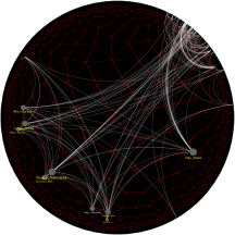
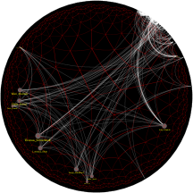
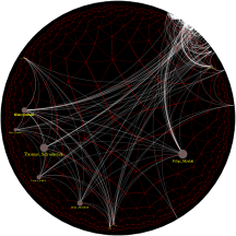
Figure 4: Visualization of the FIT 2017 coauthorship network. The root vertex is far away at 1 o’clock, the picture is centered on a specific cluster of authors. These authors collaborated on many papers; many of them have also collaborated with other authors in the network. From left to right: the network embedded with the BFKL embedder; vertices of the network are moved to the vertices of $G_{711}$; one step of the local search.

Some experiments have not been mentioned in the main paper. The local search can optimize one of the following measures: logistic log-likelihood based on the optimal values of $R$ and $T$; optimal log-likelihood where edge probability is given separately for each distance; monotonic optimal log-likelihood where the probability function has to be decreasing with larger distances; total entropy obtained by summing the optimal log-likelihood of edge and vertex placement. Non-monotonic optimal log-likelihood tends to scapegoat a fixed small distance (say, 3) and put all the pairs of close vertices which are not actually connected at that distance; monotonic optimal does not have this problem. Entropy minimization could be potentially used as a compression method; a quite good compression (46%) is obtained for the Facebook graph, though bigger graphs do not compress that well. An alternative non-local method of improving embedding is implemented, where vertices can immediately move to good locations far away (we start in the center and move in the most promising direction); this improves the log-likelihood somewhat.

The current version uses a significant amount of RAM (2.4 GB for 6 iterations the followers-2009 network which has 74946 vertices, on $G_{711}$; on $G_{710}$ it uses 1.4 GB, and on $G_{810}$ it uses 1.2 GB). It should be possible to improve this by better memory management (currently vertices and segments which are no longer used or just temporarily created are not freed), or possibly path compression.

References

- [1] interactive visualization and implementation. http://www.mimuw.edu.pl/~erykk/dhrg/.
- [2] Sergio Bermudo, José M. Rodríguez, José M. Sigarreta, and Jean-Marie Vilaire. Gromov hyperbolic graphs. Discrete Mathematics, 313(15):1575 – 1585, 2013. URL: http://www.sciencedirect.com/science/article/pii/S0012365X1300174X, doi:http://doi.org/10.1016/j.disc.2013.04.009.
- [3] Thomas Bläsius, Tobias Friedrich, Anton Krohmer, and Sören Laue. Efficient embedding of scale-free graphs in the hyperbolic plane. In European Symposium on Algorithms (ESA), pages 16:1–16:18, 2016.
- [4] Karl Bringmann, Ralph Keusch, and Johannes Lengler. Geometric inhomogeneous random graphs. Theoretical Computer Science, 2018. URL: http://www.sciencedirect.com/science/article/pii/S0304397518305309, doi:https://doi.org/10.1016/j.tcs.2018.08.014.
- [5] Karl Bringmann, Ralph Keusch, Johannes Lengler, Yannic Maus, and Anisur Rahaman Molla. Greedy routing and the algorithmic small-world phenomenom. CoRR, abs/1612.05539, 2016. URL: http://arxiv.org/abs/1612.05539.
- [6] Dorota Celińska. Information and influence in social network of Open Source community. In 9th Annual Conference of the EuroMed Academy of Business, 2016.
- [7] Dorota Celińska and Eryk Kopczyński. Programming languages in GitHub: a visualization in hyperbolic plane. In Proceedings of ICWSM 2017, Montreal, Canada, May 16-18, 2017., 2017. To appear. http://coin.wne.uw.edu.pl/dcelinska/en/pages/rogueviz-langs.html.
- [8] Bruno Courcelle. The monadic second-order logic of graphs. i. recognizable sets of finite graphs. Inf. Comput., 85(1):12–75, 1990.
- [9] Anuj Dawar and Eryk Kopczynski. Bounded degree and planar spectra. Logical Methods in Computer Science, 13(4), 2017. URL: https://doi.org/10.23638/LMCS-13(4:6)2017, doi:10.23638/LMCS-13(4:6)2017.
- [10] Georgios Gousios. The ghtorrent dataset and tool suite. In Proceedings of the 10th Working Conference on Mining Software Repositories, MSR ’13, pages 233–236, Piscataway, NJ, USA, 2013. IEEE Press. URL: http://dl.acm.org/citation.cfm?id=2487085.2487132.
- [11] Ilya Grigorik. Github Archive. https://www.githubarchive.org/, 2012.
- [12] Luca Gugelmann, Konstantinos Panagiotou, and Ueli Peter. Random hyperbolic graphs: Degree sequence and clustering. In Proceedings of the 39th International Colloquium Conference on Automata, Languages, and Programming - Volume Part II, ICALP’12, pages 573–585, Berlin, Heidelberg, 2012. Springer-Verlag. URL: http://dx.doi.org/10.1007/978-3-642-31585-5_51, doi:10.1007/978-3-642-31585-5_51.
- [13] Stephen G. Kobourov and Kevin Wampler. Non-euclidean spring embedders, pages 207–214. 2004. doi:10.1109/INFVIS.2004.49.
- [14] Eryk Kopczyński, Dorota Celińska, and Marek Čtrnáct. Hyperrogue: Playing with hyperbolic geometry. In David Swart, Carlo H. Séquin, and Kristóf Fenyvesi, editors, Proceedings of Bridges 2017: Mathematics, Art, Music, Architecture, Education, Culture, pages 9–16, Phoenix, Arizona, 2017. Tessellations Publishing. Available online at http://archive.bridgesmathart.org/2017/bridges2017-9.pdf.
- [15] John Lamping, Ramana Rao, and Peter Pirolli. A focus+context technique based on hyperbolic geometry for visualizing large hierarchies. In Proceedings of the SIGCHI Conference on Human Factors in Computing Systems, CHI ’95, pages 401–408, New York, NY, USA, 1995. ACM Press/Addison-Wesley Publishing Co. URL: http://dx.doi.org/10.1145/223904.223956, doi:10.1145/223904.223956.
- [16] Jure Leskovec and Andrej Krevl. SNAP Datasets: Stanford large network dataset collection. http://snap.stanford.edu/data, June 2014.
- [17] Maurice Margenstern. New tools for cellular automata in the hyperbolic plane. Journal of Universal Computer Science, 6(12):1226–1252, dec 2000. |http://www.jucs.org/jucs_6_12/new_tools_for_cellular—.
- [18] Maurice Margenstern. Small universal cellular automata in hyperbolic spaces: A collection of jewels, volume 4. Springer Science & Business Media, 2013.
- [19] Maurice Margenstern. Pentagrid and heptagrid: the fibonacci technique and group theory. Journal of Automata, Languages and Combinatorics, 19(1-4):201–212, 2014. URL: https://doi.org/10.25596/jalc-2014-201, doi:10.25596/jalc-2014-201.
- [20] Tamara Munzner. Exploring large graphs in 3d hyperbolic space. IEEE Computer Graphics and Applications, 18(4):18–23, 1998. URL: http://dx.doi.org/10.1109/38.689657, doi:10.1109/38.689657.
- [21] Jörg Ontrup and Helge Ritter. Hyperbolic self-organizing maps for semantic navigation. In Proceedings of the 14th International Conference on Neural Information Processing Systems: Natural and Synthetic, NIPS’01, pages 1417–1424, Cambridge, MA, USA, 2001. MIT Press. URL: http://dl.acm.org/citation.cfm?id=2980539.2980723.
- [22] Fragkiskos Papadopoulos, Rodrigo Aldecoa, and Dmitri Krioukov. Network geometry inference using common neighbors. Phys. Rev. E, 92:022807, Aug 2015. URL: https://link.aps.org/doi/10.1103/PhysRevE.92.022807, doi:10.1103/PhysRevE.92.022807.
- [23] Fragkiskos Papadopoulos, Maksim Kitsak, M. Angeles Serrano, Marian Boguñá, and Dmitri Krioukov. Popularity versus Similarity in Growing Networks. Nature, 489:537–540, Sep 2012.
- [24] Neil Robertson and P.D Seymour. Graph minors. iii. planar tree-width. Journal of Combinatorial Theory, Series B, 36(1):49 – 64, 1984. URL: http://www.sciencedirect.com/science/article/pii/0095895684900133, doi:http://dx.doi.org/10.1016/0095-8956(84)90013-3.
- [25] Moritz von Looz, Henning Meyerhenke, and Roman Prutkin. Generating Random Hyperbolic Graphs in Subquadratic Time, pages 467–478. Springer Berlin Heidelberg, Berlin, Heidelberg, 2015. URL: http://dx.doi.org/10.1007/978-3-662-48971-0_40, doi:10.1007/978-3-662-48971-0_40.
- [26] HyperRogue: programming. http://www.roguetemple.com/z/hyper/dev.php (as of Jan 27, 2017).