On the maximal directional Hilbert transform
Abstract.
For any dimension , we consider the maximal directional Hilbert transform on associated with a direction set :
The main result in this article asserts that for any exponent , there exists a positive constant such that for any finite direction set ,
where denotes the cardinality of . As a consequence, the maximal directional Hilbert transform associated with an infinite set of directions cannot be bounded on for any and any . This completes a result of Karagulyan [11], who proved a similar statement for and .
2010 Mathematics Subject Classification:
42B05, 42B15, 42B20, 42B25, 47G101. Introduction
The fundamental and ubiquitous nature of the classical one-dimensional Hilbert transform has inspired the study of a large variety of operators that share some of its distinctive features. Among the numerous higher-dimensional variants of this transform that are available in the literature, the maximal directional Hilbert transform is of notable interest, in view of its connections with several central problems in harmonic analysis, such as Carleson’s theorem on the convergence of Fourier series, estimates on maximal functions of Kakeya type and Stein’s conjecture on the Hilbert transform along Lipschitz vector fields. The treatises [15, 16] of Lacey and Li contain an extensive survey of these connections. Given a unit vector , the directional Hilbert transform is defined initially on Schwartz functions on as follows,
| (1.1) |
After a rotation that sends to the first canonical basis vector , this is essentially a tensor product of the classical Hilbert transform in with the identity operator in the remaining variables. As a result, Lebesgue mapping properties of are easy consequences of its one-dimensional counterpart [9, 10, 17]; namely, is bounded from to if and only if .
The maximal version of the operator , termed the maximal directional Hilbert transform, is the primary object of study in this article. Given a set of unit vectors and initially for a Schwartz function , it is defined to be
| (1.2) |
For finite sets , the triangle inequality gives . Thus continues to be bounded on the same Lebesgue spaces as the classical Hilbert transform, with the trivial bound
| (1.3) |
Here and throughout the paper, will denote the operator norm of from to itself. This gives rise to the following natural questions:
-
1.
To what extent can one improve upon the trivial estimate (1.3)?
-
2.
Do there exist infinite sets for which is finite for some ?
For , various aspects of question 1 above have been addressed in a large body of work [15, 5, 6, 7], encompassing results of two distinct types. With and for localized to a single frequency scale, Lacey and Li [15] have shown that the operator maps into weak , and to itself for . Here is a Schwartz function with frequency support . For finite and in the unrestricted setting (i.e., without any Fourier localization), has been studied in the more general context of maximal directional singular integral operators, co-authored in part by Demeter, Di Plinio and Parissis. For instance, the main results in [5, 6] give that for a general direction set ,
where is a constant independent of . For , this upper bound is in fact sharp for the uniformly distributed set of directions
see [5, Section 3]. On the other hand, for lacunary sets of finite order defined as in [6, 7], it has been shown that
| (1.4) |
where the constant also depends on the lacunarity order of . For , partial results with are due to Kim [13, Theorem 2]. Specifically, the estimate
is shown to hold for a direction set of cardinality in general position contained inside the positive orthant. The bound is shown to be sharp for a member of this class. In contrast, question 2 is much less studied in complete generality. Even though phrased in terms of infinite direction sets, after a finitary and quantitative reformulation it is really a question about lower bounds on for general . A result of Karagulyan [11] addresses this question in the planar setting and for , obtaining a lower bound of order for in this case. The goal of this paper is to establish this bound in far greater generality, extending it to all exponents and to all dimensions . For convenience, all logarithms below will be taken to the base 2.
Theorem 1.1.
Let be a finite set of unit vectors in with . Then for , there exists a positive constant such that
| (1.5) |
where is the cardinality of the set .
Remarks:
-
1.
Since the single-vector Hilbert transform is not bounded as an operator on or on or from to for , the theorem is trivially true for these exponents.
- 2.
-
3.
Our result extends easily to the periodic setting, with a similar proof. More explicitly, if is viewed as an operator from to , where denotes the -dimensional unit torus, then our arguments show that
for all with . The operator is unbounded for all other choices of . The construction of test functions on the torus proceeds similarly, except the convolution in (4.1) is taken on instead of .
-
4.
As a consequence of (1.5), we are able to conclude the unboundedness of for all infinite direction sets in all dimensions and on all nontrivial Lebesgue spaces. We record this below.
Theorem 1.2.
For any infinite set of unit vectors in with , the operator cannot be extended to a bounded operator on for any .
This is in sharp contrast with the behaviour of the closely related maximal directional operator
whose Lebesgue boundedness is not connected with the finitude of . For instance, the operator is known to be -bounded for all if is an infinite direction set of lacunary type in , see for example [1, 4, 18, 20, 21, 22]. For other types of direction sets that lack the feature of finite-type lacunarity, the operator is known to be unbounded on for all . This has been studied in [2, 3, 12, 14].
1.1. Notation and a preliminary reduction
We recall the equivalent Fourier-analytic formulation of the problem. For functions , we will use and to denote the Fourier transform and inverse Fourier transform respectively,
where for . If is a measurable set, we will use to denote its characteristic function, and to denote its Lebesgue measure. Given a unit vector , we will use to denote the half-space
| (1.6) |
It is well known [9, 10, 17] that the classical one-dimensional Hilbert transform can be expressed as a Fourier multiplier operator,
For the directional Hilbert transform, this means that . Accordingly, we define
Thus the boundedness of (1.2) is equivalent to that of . In particular, Theorem 1.1 is equivalent to the bound
| (1.7) |
1.2. Overview of the proof
The proof of (1.7) relies on three main components. One is geometric. More precisely, a suitable pruning and ordering of the direction set generates a finite number of mutually disjoint conic sectors , with the property that is contained in if and is disjoint from otherwise. This part of the argument is greatly simplified in the planar setting, but needs a little more care in general dimensions. This geometric ingredient is contained in Lemma 3.3. Its proof is presented in Section 6. The second ingredient is analytical. Following the general guidelines of [11] and given a fixed Lebesgue exponent , the sectors are used to construct a test function of the form , based on which (1.7) will be verified. On one hand, the function is frequency-supported in a large cube contained in the sector . Not only are these cubes disjoint from one another, they are strongly separated in a way that ensures a high degree of orthogonality among the various summands . On the other hand, the essential spatial support of is in a set , with the property that any two sets in the collection are either disjoint or nested. The critical features of this iterative construction of have been laid out in Proposition 3.2 of Section 3, and the proof of (1.7) appears here, modulo the two main estimates
| (1.8) |
the details of which are given in later sections. The proof of the estimates in (1.8) constitutes the combinatorial component of the argument. Section 5 contains the steps that lead to the first inequality in (1.8). The nested structure of the sets is best encoded as a binary tree. Combined with the stringent frequency localizations imposed on , this results in an upper bound on that is essentially comparable to . Choosing a large even integer without loss of generality allows us to express as the sum of a large number of terms of the form
Many of these terms can be ignored, based on disjoint spatial and frequency support considerations. The language of trees aids greatly in the book-keeping, identifying strings of indices that genuinely contribute to the norm. This segment of the proof has no corresponding counterpart in [11], where was always 2. In addition, the choice of modulation parameters in endows the functions Re with Haar function-like properties, termed “signed tree systems”. Basic materials concerning trees and signed tree systems have been collected in Section 2. An important fact concerning a signed tree system is proved in Section 2.3: namely, for a given and despite obvious oscillations, there exists a universal permutation of for which the largest partial sum
This choice of dictates the ordering of the sectors and is critical to the second estimate in (1.8).
2. Trees and tree systems
2.1. Trees
Given a large positive integer , we will use the following system of double-indexing to keep track of a large collection of sets and functions that arise in the sequel. Any positive integer will be identified with the pair , where
| (2.1) |
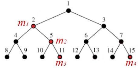
As indicated in the introduction, the language of binary trees is a convenient tool in depicting this double-indexing system. Consider a full binary tree of height , and label each tree vertex as , where is the height of the vertex (so that ranges from to ), and all vertices of height are labelled lexicographically as . Given a vertex ,
-
•
its parent can be identified as if , and
-
•
its left and right children can be identified respectively as and if .
A ray of length rooted at is a sequence of vertices where, for each , the vertex is a child of . We will also say that the vertex is a descendant of if and lies on the ray connecting to the root of the tree. In parallel to the double-numbering system in (2.1), we will use a similar convention for tree vertices, so that the vertex will be alternatively labelled by the number . We will use to denote the height of the vertex .
2.2. Tree systems
Let . We will consider finite sequences of functions , where each is a complex-valued function supported in , and use our double-numbering system from Section 2.1 to order the sequence. Thus
In many of our applications, the sequences of functions will satisfy at least one of the following properties:
-
•
For any pair with , the supports of and are either nested or disjoint, or
-
•
More specifically, if , then has constant sign on the support of (up to sets of Lebesgue measure 0).
A prototype of such a system is provided by Haar functions (cf. [19]). The abstract formulation of the property we need was given by Karagulyan in [11]. We follow the rough outline of Karagulyan’s presentation in the definitions below, but also modify the terminology and use the language of graph theory more extensively in order to accommodate the later parts of the proof that are not present in [11]. In particular, we use the term “signed tree systems” to refer to the “tree systems” of [11].
Definition 2.1.
Let , , be a finite sequence of functions, indexed as above with related by (2.1).
-
(a)
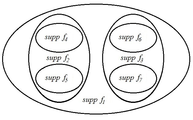
We say that is a tree system if the following holds Lebesgue almost everywhere on :
(2.2) - (b)
Figure 1 shows the relations among the supports. Clearly, every signed tree system is a tree system.
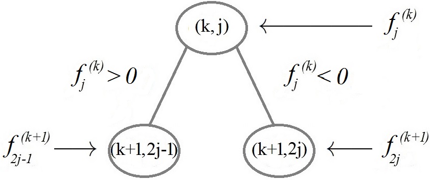
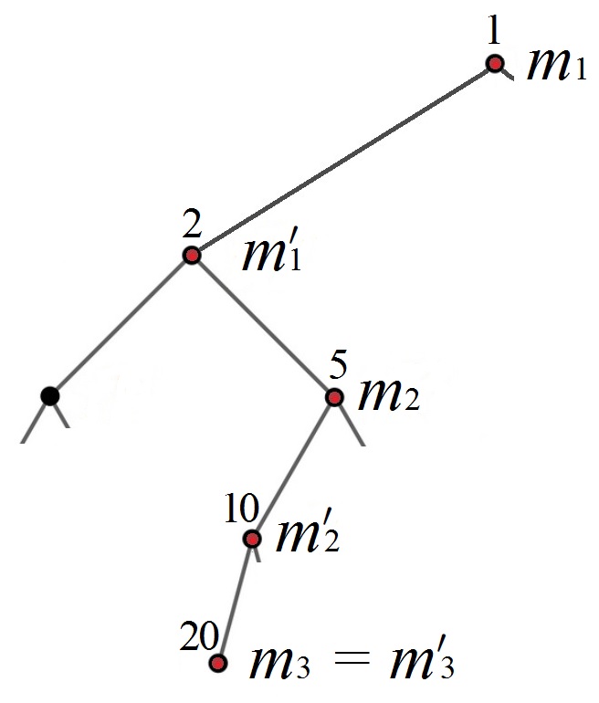
The terminology of trees adapts easily to tree systems of functions. Thus for , each function in a tree system is identified with a vertex in a complete binary tree of height , and has two children and with mutually disjoint (up to sets of measure 0) supports, both supported on . In a signed tree system, we have the additional property that the left child of is supported on the set where , and the right child is supported on the set where . Iterating this, we get the following.
Lemma 2.2.
Let be a tree system. Then for , the supports of and are either disjoint or nested. Moreover:
-
(a)
If and do not lie on the same tree ray (i.e. neither vertex is a descendant of the other), then the supports are disjoint.
-
(b)
If is a descendant of , then .
-
(c)
For each such that , there is a unique maximal ray
The ray terminates at when either or both children of take value at .
-
(d)
If is a signed tree system, then we have the additional property that encodes the sign of at :
2.3. Choice of the permutation
Here we define a special permutation of that plays a central role in the subsequent analysis. For as in (2.1), let
| (2.6) |
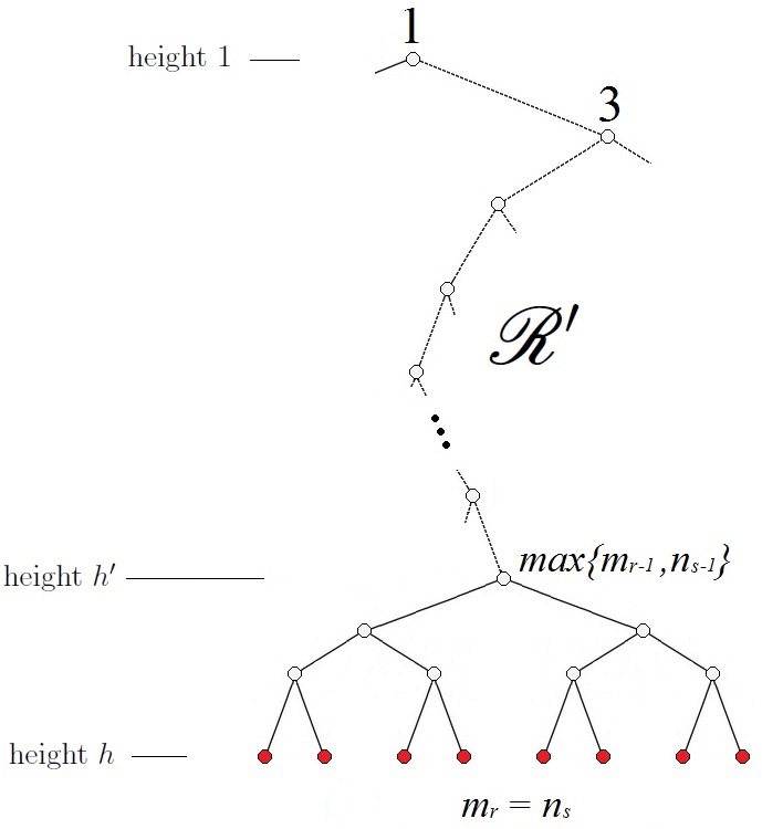
Thus , etc. Observe that a complete binary tree with levels can be represented as a planar graph so that the vertex has the -coordinate . Figure 3 illustrates this for .
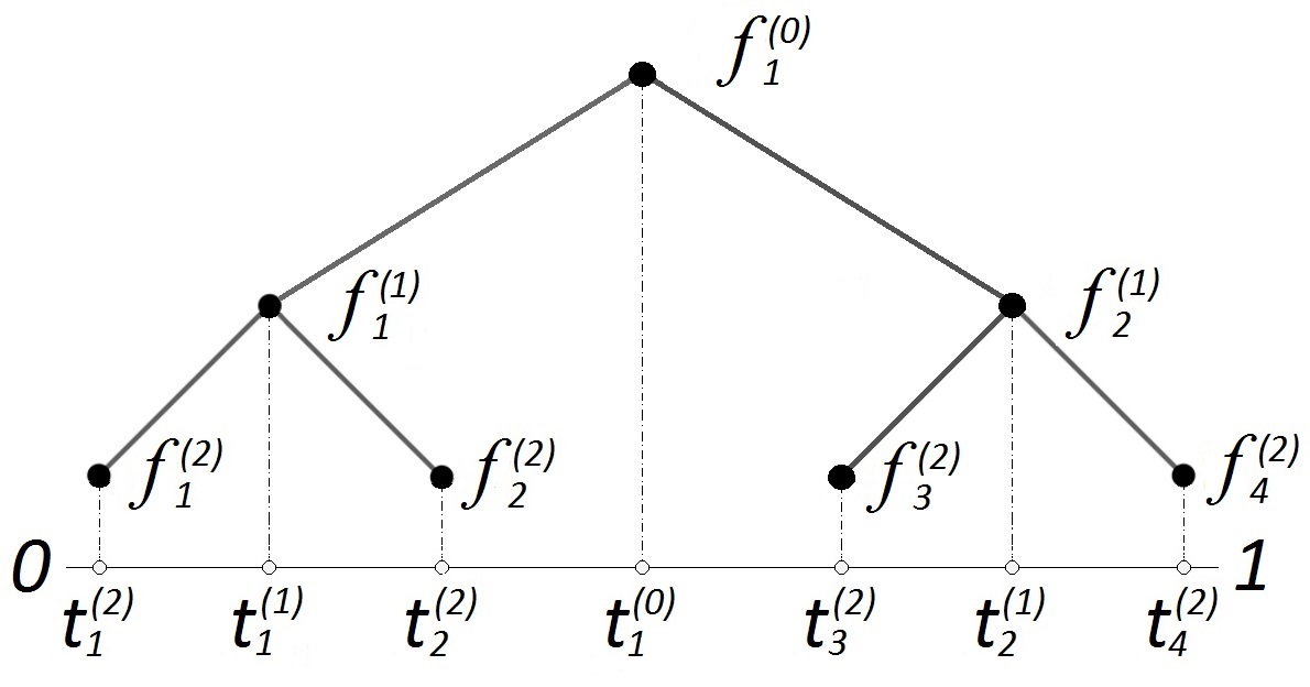
We now rearrange the sequence in increasing order. Specifically, there exists a unique permutation of the numbers , depending only on , such that
| (2.7) |
(In the example in Figure 3, we have , etc.) If are Haar functions on the line, then for each the number is the coordinate of the point where changes sign from positive to negative, and the permutation arranges the sequence in increasing order. This observation leads directly to a special case, due to Nikishin and Ulyanov [19], of Lemma 2.3 below. The generalization of the lemma to general tree systems is due to Karagulyan [11]; while Karagulyan states it only for , the same proof works in all dimensions. We follow the argument of [11], with minor corrections111Karagulyan uses instead of in his definition of . With that definition, the property (2.12) does not necessarily hold. We have rewritten that part of the proof. Alternatively, Karagulyan’s proof does work if the definition of is changed to instead. We thank an anonymous referee, as well as G. Karagulyan (private communication), for bringing that to our attention. and expository changes.
Lemma 2.3.
Proof.
In view of (2.6), we find that
| (2.9) |
Iterating over tree levels from to , and using that for any finite , we see that whenever is a descendant of in the binary tree, the corresponding numbers obey
| (2.10) |
Let , and assume that since otherwise there is nothing to prove. Define
| (2.11) |
with the convention that if the set above is empty. It follow immediately from (2.11) that for all . We claim that, furthermore,
| (2.12) |
To prove this, suppose for contradiction that there exists an such that . By (2.11), we cannot have . Let
Consider the ray defined in Lemma 2.2 (c). By definition, contains the vertex . If , then and the claim is true. Thus we are reduced to the case where and both lie on . Suppose that is a descendant of . Since , Lemma 2.2 (d) dictates that the ray turns right at , so that must be either or one of its descendants. By (2.10) and then (2.9), we have
which contradicts the assumption that and therefore . Finally, consider the case when is a descendant of . If , then turns left at , so that must be either or one of its descendants. Then, again by (2.10) and then (2.9), we have
again contradicting our assumptions.
2.3.1. An example
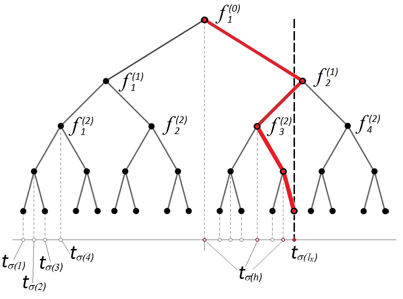
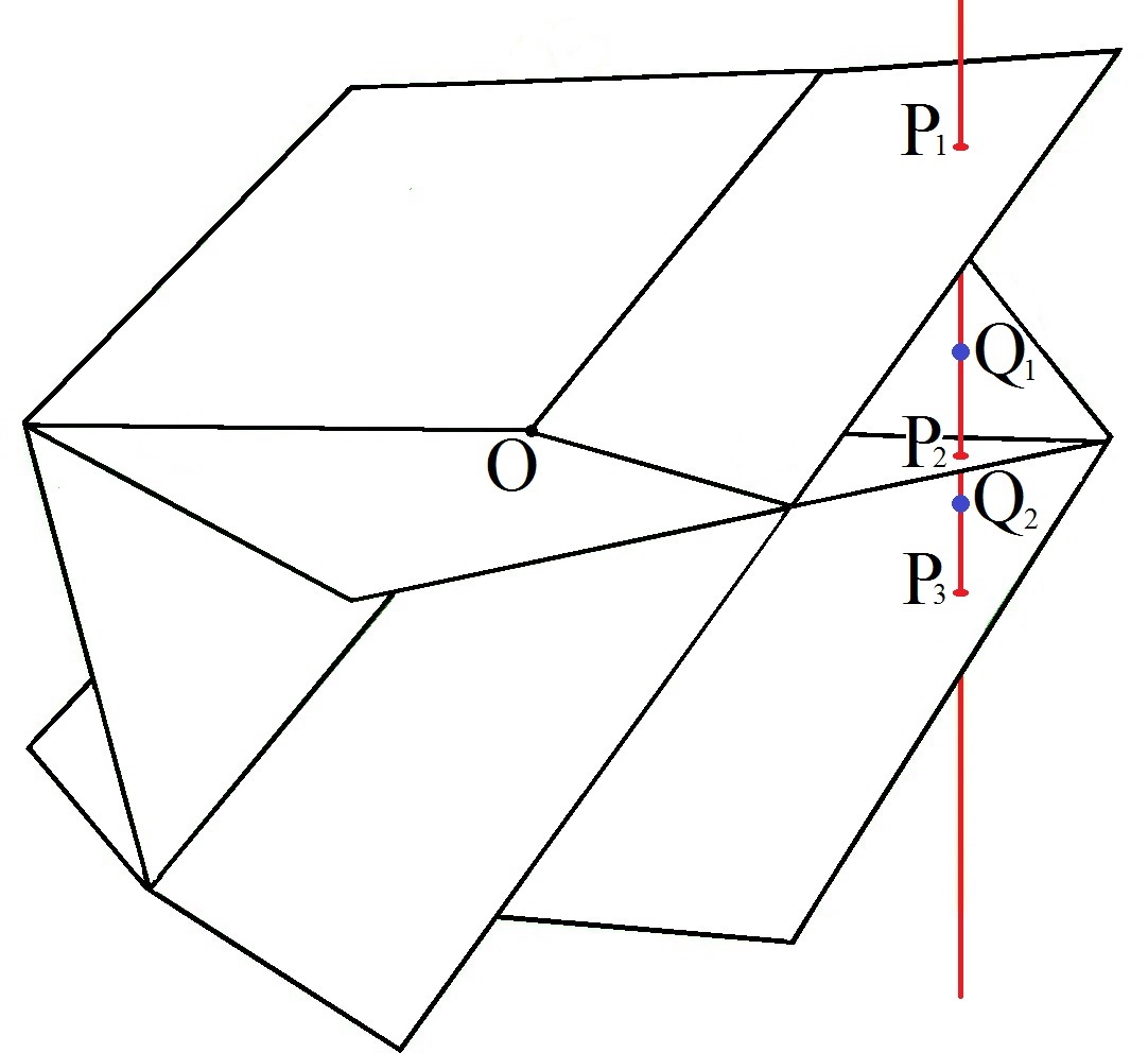
The permutation arranges in increasing order. The integer used in Lemma 2.3 then has a geometric interpretation in terms of the binary tree . Given and the ray as in Lemma 2.2(c), let be the subcollection of vertices on where the ray turns right. The maximal element is included in if and only if . Since the right child (and all its descendants) of any vertex generate larger -values than itself, the relation (2.11) defining is equivalent to the condition that . We explain the choice of in the context of an example given by Figure 4, with . Let be a point such that
Then
and hence
3. Proof of Theorem 1.1
A sector in is an open conic region in Euclidean space bounded by a finite number of hyperplanes passing through the origin. More precisely,
Definition 3.1.
Let be distinct unit vectors in , and fix an integer . A sector in is a nonempty set of the form
| (3.3) |
Note that if , then for any . Thus a sector is infinite with nonempty interior, by definition. We record in Section 3.1 two results (Proposition 3.2 and Lemma 3.3), one analytic and the other geometric, concerning sectors. These results are critical components of the proof of Theorem 1.1. We present the proof of this main theorem later in Section 3.2, modulo the two ingredients. The proofs of the two building blocks appear later in the paper (in Section 4 for Proposition 3.2 and Section 6 for Lemma 3.3).
3.1. The ingredients of the proof
Proposition 3.2.
For any choice of integer , there exist constants that depend only on and the ambient dimension and satisfy the properties listed below. Let be any finite collection of pairwise disjoint sectors in . Then there exists a corresponding sequence of smooth, integrable functions with compactly supported Fourier transforms such that:
-
(a)
for each .
-
(b)
For each ,
(3.4) - (c)
Remark: The functions given by Proposition 3.2 do not form a tree system as defined in Section 2.2. However, there are sequences of functions closely related to Re that are in fact tree systems or signed tree systems. We elaborate on these connections in Section 4 where we prove the proposition; see specifically Lemma 4.2 (a) and (c).
Lemma 3.3.
Let be a set of unit vectors in , all pointing in distinct directions. Assume that for some , and that all vectors obey , where . Then there is an ordering of vectors in , and a collection of pairwise disjoint sectors (see Definition 3.1), such that, up to sets of Lebesgue measure 0, we have for
| (3.6) |
3.2. Completion of the proof
Proof of Theorem 1.1, assuming Proposition 3.2 and Lemma 3.3.
As noted previously, it suffices to prove (1.7). Let , and let be an integer such that . Assume without loss of generality that is sufficiently large relative to , since the bound (1.7) is trivial otherwise. By rotational symmetry, we may assume (after passing to a subset of cardinality at least if necessary) that all vectors obey , where . Passing to a further subset , we may also assume that with and . Since dominates , we will henceforth work with , renaming it . Lemma 3.3 now yields an ordering of vectors in , and a collection of non-empty and pairwise disjoint sectors , such that for we have
| (3.7) |
We now apply Proposition 3.2 to the sectors for . Let , where are the functions provided by Proposition 3.2. By (b), we have
| (3.8) |
On the other hand, by Proposition 3.2(a), we have . Using this and (3.7), we get that for ,
Hence
By Proposition 3.2(c), it follows that
so that for any , we have
4. Proof of Proposition 3.2
4.1. The inductive construction of functions
Proposition 3.2 asserts the existence of certain functions ; these will be of the following form,
| (4.1) |
We pause for a moment to clarify the notation in the preceding line. Here , and is a Schwartz function on such that
The sets , the parameters and the vectors appearing in (4.1) will be specified shortly in Proposition 4.1 below using an inductive mechanism and in the sequential order
subject to the defining condition , and
| (4.2) |
As we will see, the parameter specifies the “location” and the “size” of the frequency support of . These frequency supports will obey a number of constraints, one of which is pairwise disjointness. On the other hand, the spatial support of , while not perfectly localized, is essentially contained in . The set will be shown to be nonempty and of positive measure, for every . Here for sets as well as functions, we will continue to use the double-indexing notation from Section 2, identifying with the pair as given by the relation (2.1). We will also use to denote the axis-parallel cube with centre and side length . For a multi-index , we will write ; additionally, if is a pair of such multi-indices, we will use to denote .
Proposition 4.1.
Let and be as in Proposition 3.2. For any sufficiently large , there exists a choice of large constants and vectors of large magnitude such that for all the following properties hold.
-
(a)
.
-
(b)
Given any , and any -tuple of indices , with , , we have
(4.3) Here the sum of sets denotes the Minkowski sum, where .
-
(c)
For defined as in (4.2), the vector additionally satisfies
(4.4) -
(d)
The functions and in (4.1) obey
(4.5) -
(e)
The function changes sign in . More precisely, the sets and both have positive Lebesgue measure.
Remark: Before embarking on the proof, let us rephrase the geometric condition (4.3) in an analytical form that is more convenient to check. Since
the condition (4.3) is equivalent to . If we set , and , this in turn can be written as
| (4.6) |
If , this condition specifies a set of possible that ensures the disjointness condition (4.3). We will use this to define in the sequel.
Proof of Proposition 4.1.
The proof proceeds by induction on . The sequence is an approximation to the identity; hence setting , we can choose large enough so that (4.5) holds with . Clearly . Further , so we also have . This verifies the requirements of part (d). The condition (4.3) (or equivalently (4.6)), as required by part (b), is vacuous in this case, since the only cube available so far is , and hence for any choice of multi-index . For (c), we observe that for any choice of nonzero we have
Thus any nontrivial choice of would ensure (4.4). Since , condition (e) is also trivially satisfied. With already chosen as above and keeping in mind that is a sector with unbounded interior, we can now select so that (a) holds. This completes the verification of the base case . For the inductive step, assume that we have constructed obeying all conclusions of the lemma for . Define via (4.2). Note that this is possible since and have already been set. Further, thus defined is nonempty, measurable and of positive measure since condition (e) holds for . Hence we can choose large enough so that (4.5) holds. The properties and supp follow as in the case , establishing part (d). For (c), we argue as follows: given any we have
By the Riemann-Lebesgue lemma, as . Thus for any choice of with large enough, we can ensure , resulting in (4.4). For part (b), we must choose so that (4.6) holds for all -dimensional multi-indices with and . If , this is a consequence of the induction hypothesis. We may therefore assume . This means that in the notation of (4.6). In order to ensure (4.6), we must have for ,
Since and have been determined by the previous steps of the construction, the right hand side of the relation above gives us a finite number of known cubes that must avoid for . This can be guaranteed if we assume that is large enough. To establish (e), we observe that the periodic function alternately assumes positive and negative values on parallel strips separated by distance and of comparable thickness. Thus given any open ball in , one can always choose large enough so that changes sign on the ball. Since is by definition open relative to , condition (e) follows. Note that the possible choices of so far only require the vector to be large in magnitude, with no restriction in direction. Now we choose a specific direction, and place so that we additionally have , establishing (a). This completes the inductive step and hence the proof of the proposition. ∎
4.2. Finer properties of
The algorithm described in Section 4.1 endows the resulting sets and functions with properties beyond those given in Proposition 4.1. A few of these finer properties are essential to the proof of Proposition 3.2. We record them here.
Lemma 4.2.
Proof.
Rewriting (4.2) in terms of , we get that and
Therefore, the sets and are disjoint and contained in , so that the functions form a tree system. Since the set has Legesgue measure 0, we also have (4.7). Iterating (4.7), we get that the following holds almost surely,
| (4.10) | ||||
for every . Summing over yields (4.8). We now turn to (4.9). If , the summation is over the single vertex and there is nothing to prove. If , then (4.9) follows from the same calculations as in (4.10), except we start from instead of .
The confluence of spatial and frequency localization built into the definition of results in a high degree of orthogonality amongst them. This interaction is manifested in the -norms of their sums, for large exponents . The following proposition, which offers an estimate of this norm, is a critical component in the proof of Proposition 3.2(b). The proof of the proposition is nontrivial and is relegated to Section 5.
Proposition 4.3.
Assuming this, the proof of Proposition 3.2 is completed in the next subsection.
4.3. Proof of Proposition 3.2
Proof.
Since supp, part (a) of the proposition follows from Proposition 4.1(a). Let us turn to (b). Given that , the desired conclusion follows from the log-convexity of Lebesgue norms, provided we have the correct estimates at the endpoints and . Proposition 4.3 asserts the necessary bound for . Our claim is that the bound for follows from the same proposition. The following chain of inequalities establishes this claim:
The third and the sixth inequality in the sequence above uses the error bound (4.5) proved in Proposition 4.1(d). The fourth inequality follows from the fact that is supported on , and hence by Hölder’s inequality. The last inequality follows from the main estimate (4.11) in Proposition 4.3. The triangle inequality is used throughout. This completes the proof of (b). It remains to prove (c). Recall from Lemma 4.2(c) that is a signed tree system. Hence by Lemma 2.3 for signed tree systems, we have
for all , where . The last inequality above follows from (2.8), the rest from the triangle inequality. We will show that
| (4.12) | ||||
| (4.13) |
For large , this would ensure (3.5) and complete the proof, with constants and , for instance. To prove (4.12), let us set . On one hand, by Proposition 4.1(c),
Summing over all and using (4.8) in Lemma 4.2, we obtain
| (4.14) |
On the other hand,
| (4.15) |
Set . Combining (4.14) and (4.15), we see that
This shows that , establishing (4.12). Regarding (4.13), we make use of (4.5) to deduce that
Therefore, by Chebyshev’s inequality
| (4.16) |
which proves our claim (4.13) for sufficiently large. ∎
5. Norm estimate: Proof of Proposition 4.3
This section is given over to the estimation of the norm of the function , with the summands defined as in Proposition 4.1. Parts of the argument are highly combinatorial, involving summations over index sets whose members are long sequences of integers. Two previously introduced tools will continue to be useful for book-keeping purposes; namely, the double-indexing notation relating with the pair as in (2.1), and the language of trees as described in Section 2. We begin by setting up some supplementary notation that will be convenient for handling sums over large index sets later on.
5.1. Notation
5.1.1. Small errors
For any two quantities and depending on , we will write if , where the multiplicative constant and the exponent may depend on and , and may change from line to line but remain independent of . Both and will always be sufficiently large. In our applications, will depend on the large constant from Proposition 4.1. Assuming that was chosen large enough, we will always be able to ensure that . The notation will be used to mean , with the same conditions on the constant as above.
5.1.2. Grouping of vectors of vertices
Our main estimate will be proved by expanding the norm of as a sum of integrals of the form
| (5.1) |
with , then grouping these integrals appropriately to obtain cancellations and simplifications. The notation introduced in this subsection will facilitate that process.
Given an integer exponent and an integer dimension , we define a multiplicity vector for the exponent of length to be of the form
The use of a multiplicity vector allows us to rewrite a -long integer vector with some possibly coincident entries in “collapsed form”. For instance, all such sequences with distinct entries, where the -th smallest element occurs with frequency , can be gathered into a single collection, as explained below. Given integers , we set
| (5.2) |
Observe that for every , there exist -dimensional vectors such that occurs in the string exactly times for each . For example, we can take to be , which is by definition a -long vector whose first entries are , the next entries are , and so on. The relevance of lies in the following partition of the index set:
| (5.3) |
Right now, an element of is a 2-tuple , whose first component is a multi-index and whose second component is an -long multiplicity vector for . The number of choices of for a fixed and is bounded by a constant depending only on and independent of (and hence ), whereas ranges over an index set of cardinality , which is typically much larger. For the quantitative bounds that we seek, it is therefore no loss of generality to work with a fixed multiplicity vector at a time. In order to keep track of the collection of all multi-indices that generate elements of for a fixed multiplicity, we define
| (5.4) |
which is in effect the -fibre of . We will also need to stratify pairs of vectors according to the position of their combined maximal element in the binary tree. With that in mind and given multiplicity vectors of length for the exponents respectively, we set
| (5.5) |
Recall that denotes the height of the vertex in the binary tree . The parameters occurring in the argument of (5.5) will be suppressed if they are clear from the context.
Two special subclasses of will be important for our analysis. They are:
| (5.6) | ||||
| (5.7) |
Figures 5 and 6 depict examples of multi-indices that lie in these special subclasses.
5.2. Main steps
The relevance of the aforementioned notation in the context of the norm estimation problem is clarified in the following sequence of lemmas, which provides the key ingredients.
Lemma 5.1.
Let , with given by (4.1) in Section 4. Then
| (5.8) |
To explain the notation in the above line,
-
•
The outer sum ranges over all choices of positive integers and all choices of multiplicity vectors for the exponent of lengths and respectively.
-
•
The constants depend only on and are independent of ; specifically
-
•
Given ,
(5.9)
We will continue to use the notation (5.9) even if are multiplicity vectors for different exponents.
Lemma 5.2.
Fix , and two multiplicity vectors for integer exponents of lengths respectively. Then the following conclusions hold:
- (a)
-
(b)
If , then . The converse is also true. For such , we have
(5.13) -
(c)
As a consequence, , where
Lemma 5.3.
5.3. Proof of Proposition 4.3
Proof.
We complete the proof of the proposition assuming the three lemmas above. In view of Lemma 5.1, is given by (5.8). The number of summands in the outer sum on the right hand side of the equation (5.8) depends only on ; hence it suffices to show that
for every fixed choice of integers and for each choice of multiplicity vectors for the exponent of lengths respectively and . Combining Lemma 5.2(c) with Lemma 5.3, we find that
and otherwise, completing the proof. ∎
5.4. Proof of Lemma 5.1
Proof.
We start by expanding the -norm of as follows,
| (5.15) |
where the summation ranges over all -dimensional multi-indices
The entries in (and hence also ) need not be distinct. However, in view of (5.3) and the discussion leading up to it, for every there exist
-
•
a unique integer ,
-
•
a multiplicity vector of length for , and
-
•
a choice of defined as in (5.4),
such that is a permutation of , i.e., , and occurs exactly times in . Thus
Further, given a fixed choice of and , there are exactly -many possibilities of that correspond to the same choice of . Grouping the sum in (5.15) using these multiplicities, we obtain
| (5.16) |
where has been defined in (5.9), the outer sum is as in the statement of the lemma and the inner sum ranges over all multi-indices . Finally, we note that
Decomposing the inner sum in (5.16) based on therefore leads to (5.8). ∎
5.5. Proof of Lemma 5.2
Proof.
Part (a) of the lemma is based on an iterative application of the following estimate: for any measurable function with , (4.5) gives
| (5.17) |
We use this estimate to successively peel away each factor occurring in , replacing it by instead. Specifically, starting with any , we can write
is a product of factors. As a result,
| (5.18) | ||||
The last step above uses (5.17) with , which is bounded by 1 according to Proposition 4.1(d). Iterating the argument in (5.18) exactly times (and using (5.17) with a different choice of at each stage), we are able to remove all factors and are left with the integrand . This is the desired claim (5.10). Regarding (b), we recall from Lemma 4.2(a) that the family of functions is a tree system. In particular, for any two indices , the sets and (which are non-empty by Proposition 4.1) are either disjoint or nested. Their intersection is nonempty precisely when , which in turn happens if and only if is an ancestor of , when represented as vertices on the binary tree . Thus is nonempty if and only if there is a strict lineage among the indices in , i.e., for any two entries of , one is either an ancestor or a descendant of the other. In other words, the vertices of lie on a ray of , i.e. . It follows from the definition (4.2) and more precisely from Lemma 4.2(a) that the sets shrink as proceeds down a ray of the tree. Thus must equal , where is the terminating vertex of the ray that contains the indices of . This leads to (5.13). Part (c) is obtained by adding the estimates deduced in the first two parts of the lemma over all . The verification is left to the interested reader. Note the importance of the large constant in this step, as a result of which the error implicit in remains small even after summing over terms. ∎
5.6. Proof of Lemma 5.3
Proof.
In view of Lemma 5.2(c), we know that . To establish the first relation in (5.14), it therefore suffices to show that . This in turn will follow from the estimate below. For any choice of ,
| (5.19) | ||||
By Lemma 5.2(a) combined with Plancherel’s theorem, we obtain
where we use the notation to denote the -fold convolution of with itself. The integrand on the right hand side above is supported in the set
By (4.3) in Lemma 4.1(b), this intersection is empty unless and , establishing (5.19). For the second relation in (5.14), we will rely on the following recursion formula, to be proven shortly:
| (5.20) | ||||
are multiplicity vectors of lengths and for the exponents and respectively. Assuming this for now, the proof is completed as follows. First suppose that , and that is the smallest index such that . If , then directly from (5.19). If , then a -fold iteration of (5.20) yields
| (5.21) |
with , . Note that and are multiplicity vectors of length and for the exponents and respectively, where . Since , we can apply (5.19), with the parameters in (5.19) replaced by respectively. This leads to the estimate
After summing over all the indices in the relevant collection , the above relation yields that . This in turn shows that the iterated sum in (5.21) is also , since the number of summands is at most . This completes the proof for . On the other hand, if , then iterating (5.20) times we find that
At the penultimate step above, we have computed for any ,
The last step is a consequence of Lemma 4.2(b) with . This completes the proof. ∎
5.7. Summing over subtrees: Proof of (5.20)
Proof.
Any can be written as , where
and is a string of vertices lying on a ray in and terminating in the vertex of height . As such, can be partitioned as
This results in a corresponding decomposition for the sum representing :
| (5.22) | ||||
In all the sums above, ranges over . For a given , the summation index ranges over descendants of of height in . This has been described in Figure 7. In the third equality, the summation in follows from the property that is a tree system. In particular we have invoked Lemma 4.2(b) with , along with (5.13). ∎
6. Proof of Lemma 3.3
In this section we prove the geometric result used in the proof of the theorem in Section 3. Recall that . We restate the lemma below for easier referencing.
Lemma 6.1.
Let be a set of unit vectors in , all pointing in distinct directions. Assume that for some , and that all vectors obey , where . Then there is an ordering of vectors in , and a collection of pairwise disjoint sectors (see Definition 3.1), such that, up to sets of Lebesgue measure 0, we have for
| (6.1) |
Proof.
For a unit vector , we will use to denote the hyperplane . By a slight abuse of notation, we will also write . For , let be the line
Since for all , the line is not parallel to any of the corresponding hyperplanes . Moreover, for all outside of an exceptional set of -dimensional Lebesgue measure 0, it intersects these hyperplanes at distinct points. Fix one such point , and let be the intersection points listed in the order of decreasing so that . We then label the vectors in as so that
and define
Then if and if , so that we have (6.1). It is also clear from the definition that the sectors are pairwise disjoint. To see that they are non-empty, it suffices to check that for , where for some choice of scalars obeying . Indeed, for any and , we have
| which is |
Thus if and if , proving the claim. ∎
Remark: We point out the main distinctions of Lemma 3.3 in general dimensions relative to its planar counterpart in [11]. In dimension two, the hyperplanes are lines passing through the origin. Any conical sector is bounded by exactly two such lines. Thus lines of the form divide a half-plane into exactly sectors that admit an obvious ordering simply by moving in a clockwise direction. In , hyperplanes intersect in more complicated ways. A conical sector may be bounded by a number of hyperplanes far greater than . Furthermore, a collection of vectors in typically generates many more than sectors, among which there is no natural “global” ordering. In Lemma 3.3, we choose, from the collection of all sectors, a subset of size , on which we impose a natural ordering, in terms of the height of the sector above a fixed point in the -hyperplane.
7. Acknowledgement
The authors thank two anonymous referees for their careful reading of the manuscript and valuable suggestions that improved the presentation. This work was supported by NSERC Discovery Grants 22R80520 and 22R82900.
References
- [1] A. Alfonseca, Strong type inequalities and an almost-orthogonality principle for families of maximal operators along directions in , J. London Math. Soc. (2) 67 (2003), no. 1, 208–218.
- [2] M. Bateman, Kakeya sets and directional maximal operators in the plane, Duke Math. J. 147 (2009), no. 1, 55–77.
- [3] M. Bateman and N. H. Katz, Kakeya sets in Cantor directions, Math. Res. Lett. 15 (2008), no. 1, 73–81.
- [4] A. Carbery, Differentiation in lacunary directions and an extension of the Marcinkiewicz multiplier theorem, Ann. Inst. Fourier (Grenoble) 38 (1988), no. 1, 157–168.
- [5] C. Demeter, Singular integrals along N directions in , Proc. Amer. Math. Soc. 138 (2010), no. 12, 4433–4442.
- [6] C. Demeter and F. Di Plinio, Logarithmic bounds for maximal directional singular integrals in the plane, J. Geom. Anal. 24 (2014), no. 1, 375–416.
- [7] F. Di Plinio and I. Parissis, A sharp estimate for the Hilbert transform along finite order lacunary sets of directions, (2017) to appear in Israel J. Math., preprint available at https://arxiv.org/abs/1704.02918.
- [8] F. Di Plinio and I. Parissis, On the maximal directional Hilbert transform in three dimensions (2017), available at https://arxiv.org/abs/1712.02673.
- [9] L. Grafakos, Classical Fourier analysis, 3rd ed., Graduate Texts in Mathematics 249, Springer-Verlag, New York, 2014.
- [10] L. Grafakos, Modern Fourier analysis, 3rd ed., Graduate Texts in Mathematics 250, Springer-Verlag, New York, 2014.
- [11] G. A. Karagulyan, On unboundedness of maximal operators for directional Hilbert transforms, Proc. Amer. Math. Soc. 135 (2007), no. 10, 3133–3141.
- [12] N. H. Katz, Maximal operators over arbitrary sets of directions. Duke Math. J. 97 (1999), no. 1, 67–79.
- [13] J. Kim, Sharp bound of maximal Hilbert transforms over arbitrary sets of directions, J. Math. Anal. Appl. 335 (2007), no. 1, 56–63.
- [14] E. Kroc and M. Pramanik, Kakeya-type sets over Cantor sets of directions in , J. Fourier Anal. Appl. 22 (2016), no. 3, 623–674.
- [15] M. Lacey and X. Li, Maximal theorems for the directional Hilbert transform on the plane, Trans. Amer. Math. Soc. 358 (2006), no. 9, 4099–4117.
- [16] M. Lacey and X. Li, On a conjecture of E. M. Stein on the Hilbert transform on vector fields, Mem. Amer. Math. Soc. 205 (2010), no. 965.
- [17] C. Muscalu and W. Schlag, Classical and Multilinear Harmonic Analysis, Vol. I, Cambridge Studies in Advanced Mathematics, 137, Cambridge University Press, Cambridge, 2013.
- [18] A. Nagel, E.M. Stein and S. Wainger, Differentiation in lacunary directions, Proc. Nat. Acad. Sci. USA 75 (1978), no. 3, 1060–1062.
- [19] E.M. Nikishin and P.L. Ulyanov, On absolute and unconditional convergence, Uspechi Math. Nauk. 22 (1967), no. 3, 240–242 (in Russian).
- [20] J. Parcet and K. M. Rogers, Differentiation of integrals in higher dimensions, Proc. Nat. Acad. Sci. USA 110 (2013), no. 13, 4941–4944.
- [21] J. Parcet and K. M. Rogers, Directional maximal operators and lacunarity in higher dimensions, Amer. J. Math. 137 (2015), no. 6, 1535–1557.
- [22] P. Sjögren and P. Sjölin, Littlewood-Paley decompositions and Fourier multipliers with singularities on certain sets. Ann. Inst. Fourier (Grenoble) 31 (1981), no. 1, vii, 157–175.
Izabella Łaba
University of British Columbia, Vancouver, Canada.
Electronic address: ilaba@math.ubc.ca
Alessandro Marinelli
University of British Columbia, Vancouver, Canada.
Electronic address: marine7@math.ubc.ca
Malabika Pramanik
University of British Columbia, Vancouver, Canada.
Electronic address: malabika@math.ubc.ca