Context-Free Path Querying by Matrix Multiplication

Abstract.

Graph data models are widely used in many areas, for example, bioinformatics, graph databases. In these areas, it is often required to process queries for large graphs. Some of the most common graph queries are navigational queries. The result of query evaluation is a set of implicit relations between nodes of the graph, i.e. paths in the graph. A natural way to specify these relations is by specifying paths using formal grammars over the alphabet of edge labels. An answer to a context-free path query in this approach is usually a set of triples $(A,m,n)$ such that there is a path from the node $m$ to the node $n$, whose labeling is derived from a non-terminal $A$ of the given context-free grammar. This type of queries is evaluated using the relational query semantics. Another example of path query semantics is the single-path query semantics which requires presenting a single path from the node $m$ to the node $n$, whose labeling is derived from a non-terminal $A$ for all triples $(A,m,n)$ evaluated using the relational query semantics. There is a number of algorithms for query evaluation which use these semantics but all of them perform poorly on large graphs. One of the most common technique for efficient big data processing is the use of a graphics processing unit (GPU) to perform computations, but these algorithms do not allow to use this technique efficiently. In this paper, we show how the context-free path query evaluation using these query semantics can be reduced to the calculation of the matrix transitive closure. Also, we propose an algorithm for context-free path query evaluation which uses relational query semantics and is based on matrix operations that make it possible to speed up computations by using a GPU.

1. Introduction

Graph data models are widely used in many areas, for example, bioinformatics (Anderson et al., 2013), graph databases (Mendelzon and Wood, 1995). In these areas, it is often required to process queries for large graphs. The most common among graph queries are navigational queries. The result of query evaluation is a set of implicit relations between nodes of the graph, i.e. paths in the graph. A natural way to specify these relations is by specifying paths using formal grammars (regular expressions, context-free grammars) over the alphabet of edge labels. Context-free grammars are actively used in graphs queries because of the limited expressive power of regular expressions.

The result of context-free path query evaluation is usually a set of triples $(A,m,n)$ such that there is a path from the node $m$ to the node $n$, whose labeling is derived from a non-terminal $A$ of the given context-free grammar. This type of query is evaluated using the relational query semantics (Hellings, 2014). Another example of path query semantics is the single-path query semantics (Hellings, 2015) which requires presenting a single path from the node $m$ to the node $n$ whose labeling is derived from a non-terminal $A$ for all triples $(A,m,n)$ evaluated using the relational query semantics. There is a number of algorithms for context-free path query evaluation using these semantics (Grigorev and Ragozina, 2016; Hellings, 2014; Zhang et al., 2016; Sevon and Eronen, 2008).

Existing algorithms for context-free path query evaluation w.r.t. these semantics demonstrate poor performance when applied to big data. One of the most common technique for efficient big data processing is GPGPU (General-Purpose computing on Graphics Processing Units), but these algorithms do not allow to use this technique efficiently. The algorithms for context-free language recognition had a similar problem until Valiant (Valiant, 1975) proposed a parsing algorithm which computes a recognition table by computing matrix transitive closure. Thus, the active use of matrix operations (such as matrix multiplication) in the process of a transitive closure computation makes it possible to efficiently apply GPGPU computing techniques (Che et al., 2016).

We address the problem of creating an algorithm for context-free path query evaluation using the relational and the single-path query semantics which allows us to speed up computations with GPGPU by using the matrix operations.

The main contribution of this paper can be summarized as follows:

• We show how the context-free path query evaluation w.r.t. the relational and the single-path query semantics can be reduced to the calculation of matrix transitive closure.

• We introduce an algorithm for context-free path query evaluation w.r.t. the relational query semantics which is based on matrix operations that make it possible to speed up computations by means of GPGPU.

• We provide a formal proof of correctness of the proposed algorithm.

• We show the practical applicability of the proposed algorithm by running different implementations of our algorithm on real-world data.

2. Preliminaries

In this section, we introduce the basic notions used throughout the paper.

Let $\Sigma$ be a finite set of edge labels. Define an edge-labeled directed graph as a tuple $D=(V,E)$ with a set of nodes $V$ and a directed edge-relation $E\subseteq V\times\Sigma\times V$. For a path $\pi$ in a graph $D$, we denote the unique word obtained by concatenating the labels of the edges along the path $\pi$ as $l(\pi)$. Also, we write $n\pi m$ to indicate that a path $\pi$ starts at the node $n\in V$ and ends at the node $m\in V$.

Following Hellings (Hellings, 2014), we deviate from the usual definition of a context-free grammar in Chomsky Normal Form (Chomsky, 1959) by not including a special starting non-terminal, which will be specified in the path queries to the graph. Since every context-free grammar can be transformed into an equivalent one in Chomsky Normal Form and checking that an empty string is in the language is trivial it is sufficient to consider only grammars of the following type. A context-free grammar is a triple $G=(N,\Sigma,P)$, where $N$ is a finite set of non-terminals, $\Sigma$ is a finite set of terminals, and $P$ is a finite set of productions of the following forms:

• $A\rightarrow BC$, for $A,B,C\in N$,

• $A\rightarrow x$, for $A\in N$ and $x\in\Sigma$.

Note that we omit the rules of the form $A\rightarrow\varepsilon$, where $\varepsilon$ denotes an empty string. This does not restrict the applicability of our algorithm because only the empty paths $m\pi m$ correspond to an empty string $\varepsilon$.

We use the conventional notation $A\xrightarrow{*}w$ to denote that a string $w\in\Sigma^{*}$ can be derived from a non-terminal $A$ by some sequence of applications of the production rules from $P$. The language of a grammar $G=(N,\Sigma,P)$ with respect to a start non-terminal $S\in N$ is defined by

$$L(G_{S})=\{w\in\Sigma^{*}~{}|~{}S\xrightarrow{*}w\}.$$

For a given graph $D=(V,E)$ and a context-free grammar $G=(N,\Sigma,P)$, we define context-free relations $R_{A}\subseteq V\times V$, for every $A\in N$, such that

$$R_{A}=\{(n,m)~{}|~{}\exists n\pi m~{}(l(\pi)\in L(G_{A}))\}.$$

We define a binary operation $(~{}\cdot~{})$ on arbitrary subsets $N_{1},N_{2}$ of $N$ with respect to a context-free grammar $G=(N,\Sigma,P)$ as

$$N_{1}\cdot N_{2}=\{A~{}|~{}\exists B\in N_{1},\exists C\in N_{2}\text{ such that }(A\rightarrow BC)\in P\}.$$

Using this binary operation as a multiplication of subsets of $N$ and union of sets as an addition, we can define a matrix multiplication, $a\times b=c$, where $a$ and $b$ are matrices of a suitable size that have subsets of $N$ as elements, as

$$c_{i,j}=\bigcup^{n}_{k=1}{a_{i,k}\cdot b_{k,j}}.$$

According to Valiant (Valiant, 1975), we define the transitive closure of a square matrix $a$ as $a^{+}=a^{(1)}_{+}\cup a^{(2)}_{+}\cup\cdots$ where $a^{(1)}_{+}=a$ and

$$a^{(i)}_{+}=\bigcup^{i-1}_{j=1}{a^{(j)}_{+}\times a^{(i-j)}_{+}},~{}i\geq 2.$$

We enumerate the positions in the input string $s$ of Valiant’s algorithm from 0 to the length of $s$. Valiant proposes the algorithm for computing this transitive closure only for upper triangular matrices, which is sufficient since for Valiant’s algorithm the input is essentially a directed chain and for all possible paths $n\pi m$ in a directed chain $n<m$. In the context-free path querying input graphs can be arbitrary. For this reason, we introduce an algorithm for computing the transitive closure of an arbitrary square matrix.

For the convenience of further reasoning, we introduce another definition of the transitive closure of an arbitrary square matrix $a$ as $a^{cf}=a^{(1)}\cup a^{(2)}\cup\cdots$ where $a^{(1)}=a$ and

$$a^{(i)}=a^{(i-1)}\cup(a^{(i-1)}\times a^{(i-1)}),~{}i\geq 2.$$

To show the equivalence of these two definitions of transitive closure, we introduce the partial order $\succeq$ on matrices with the fixed size which have subsets of $N$ as elements. For square matrices $a,b$ of the same size, we denote $a\succeq b$ iff $a_{i,j}\supseteq b_{i,j}$, for every $i,j$. For these two definitions of transitive closure, the following lemmas and theorem hold.

Lemma 2.1.

Let $G=(N,\Sigma,P)$ be a grammar, let $a$ be a square matrix. Then $a^{(k)}\succeq a^{(k)}_{+}$ for any $k\geq 1$.

Proof.

(Proof by Induction)

Basis: The statement of the lemma holds for $k=1$, since

$$a^{(1)}=a^{(1)}_{+}=a.$$

Inductive step: Assume that the statement of the lemma holds for any $k\leq(p-1)$ and show that it also holds for $k=p$ where $p\geq 2$. For any $i\geq 2$

$$a^{(i)}=a^{(i-1)}\cup(a^{(i-1)}\times a^{(i-1)})\Rightarrow a^{(i)}\succeq a^{(i-1)}.$$

Hence, by the inductive hypothesis, for any $i\leq(p-1)$

$$a^{(p-1)}\succeq a^{(i)}\succeq a^{(i)}_{+}.$$

Let $1\leq j\leq(p-1)$. The following holds

$$(a^{(p-1)}\times a^{(p-1)})\succeq(a^{(j)}_{+}\times a^{(p-j)}_{+}),$$

since $a^{(p-1)}\succeq a^{(j)}_{+}$ and $a^{(p-1)}\succeq a^{(p-j)}_{+}$. By the definition,

$$a^{(p)}_{+}=\bigcup^{p-1}_{j=1}{a^{(j)}_{+}\times a^{(p-j)}_{+}}$$

and from this it follows that

$$(a^{(p-1)}\times a^{(p-1)})\succeq a^{(p)}_{+}.$$

By the definition,

$$a^{(p)}=a^{(p-1)}\cup(a^{(p-1)}\times a^{(p-1)})\Rightarrow a^{(p)}\succeq(a^{(p-1)}\times a^{(p-1)})\succeq a^{(p)}_{+}$$

and this completes the proof of the lemma. ∎

Lemma 2.2.

Let $G=(N,\Sigma,P)$ be a grammar, let $a$ be a square matrix. Then for any $k\geq 1$ there is $j\geq 1$, such that $(\bigcup^{j}_{i=1}{a^{(i)}_{+}})\succeq a^{(k)}$.

Proof.

(Proof by Induction)

Basis: For $k=1$ there is $j=1$, such that

$$a^{(1)}_{+}=a^{(1)}=a.$$

Thus, the statement of the lemma holds for $k=1$.

Inductive step: Assume that the statement of the lemma holds for any $k\leq(p-1)$ and show that it also holds for $k=p$ where $p\geq 2$. By the inductive hypothesis, there is $j\geq 1$, such that

$$(\bigcup^{j}_{i=1}{a^{(i)}_{+}})\succeq a^{(p-1)}.$$

By the definition,

$$a^{(2j)}_{+}=\bigcup^{2j-1}_{i=1}{a^{(i)}_{+}\times a^{(2j-i)}_{+}}$$

and from this it follows that

$$(\bigcup^{2j}_{i=1}{a^{(i)}_{+}})\succeq(\bigcup^{j}_{i=1}{a^{(i)}_{+}})\times(\bigcup^{j}_{i=1}{a^{(i)}_{+}})\succeq(a^{(p-1)}\times a^{(p-1)}).$$

The following holds

$$(\bigcup^{2j}_{i=1}{a^{(i)}_{+}})\succeq a^{(p)}=a^{(p-1)}\cup(a^{(p-1)}\times a^{(p-1)}),$$

since

$$(\bigcup^{2j}_{i=1}{a^{(i)}_{+}})\succeq(\bigcup^{j}_{i=1}{a^{(i)}_{+}})\succeq a^{(p-1)}$$

and

$$(\bigcup^{2j}_{i=1}{a^{(i)}_{+}})\succeq(a^{(p-1)}\times a^{(p-1)}).$$

Therefore there is $2j$, such that

$$(\bigcup^{2j}_{i=1}{a^{(i)}_{+}})\succeq a^{(p)}$$

and this completes the proof of the lemma. ∎

Theorem 1.

Let $G=(N,\Sigma,P)$ be a grammar, let $a$ be a square matrix. Then $a^{+}=a^{cf}$.

Proof.

By the lemma 2.1, for any $k\geq 1$, $a^{(k)}\succeq a^{(k)}_{+}$. Therefore

$$a^{cf}=a^{(1)}\cup a^{(2)}\cup\cdots\succeq a^{(1)}_{+}\cup a^{(2)}_{+}\cup\cdots=a^{+}.$$

By the lemma 2.2, for any $k\geq 1$ there is $j\geq 1$, such that

$$(\bigcup^{j}_{i=1}{a^{(i)}_{+}})\succeq a^{(k)}.$$

Hence

$$a^{+}=(\bigcup^{\infty}_{i=1}{a^{(i)}_{+}})\succeq a^{(k)},$$

for any $k\geq 1$. Therefore

$$a^{+}\succeq a^{(1)}\cup a^{(2)}\cup\cdots=a^{cf}.$$

Since $a^{cf}\succeq a^{+}$ and $a^{+}\succeq a^{cf}$,

$$a^{+}=a^{cf}$$

and this completes the proof of the theorem. ∎

Further, in this paper, we use the transitive closure $a^{cf}$ instead of $a^{+}$ and, by the theorem 1, an algorithm for computing $a^{cf}$ also computes Valiant’s transitive closure $a^{+}$.

3. Related works

Problems in many areas can be reduced to one of the formal-languages-constrained path problems (Barrett et al., 2000). For example, various problems of static code analysis (Bastani et al., 2015; Xu et al., 2009) can be formulated in terms of the context-free language reachability (Reps, 1998) or in terms of the linear conjunctive language reachability (Zhang and Su, 2017).

One of the well-known problems in the area of graph database analysis is the language-constrained path querying. For example, the regular language constrained path querying (Reutter et al., 2017; Fan et al., 2011; Abiteboul and Vianu, 1997; Nolé and Sartiani, 2016), and the context-free language constrained path querying.

There are a number of solutions (Hellings, 2014; Sevon and Eronen, 2008; Zhang et al., 2016) for context-free path query evaluation w.r.t. the relational query semantics, which employ such parsing algorithms as CYK (Kasami, 1965; Younger, 1967) or Earley (Grune and Jacobs, 2006). Other examples of path query semantics are single-path and all-path query semantics. The all-path query semantics requires presenting all possible paths from node $m$ to node $n$ whose labeling is derived from a non-terminal $A$ for all triples $(A,m,n)$ evaluated using the relational query semantics. Hellings (Hellings, 2015) presented algorithms for the context-free path query evaluation using the single-path and the all-path query semantics. If a context-free path query w.r.t. the all-path query semantics is evaluated on cyclic graphs, then the query result can be an infinite set of paths. For this reason, in (Hellings, 2015), annotated grammars are proposed as a possible solution.

In (Grigorev and Ragozina, 2016), the algorithm for context-free path query evaluation w.r.t. the all-path query semantics is proposed. This algorithm is based on the generalized top-down parsing algorithm — GLL (Scott and Johnstone, 2010). This solution uses derivation trees for the result representation which is more native for grammar-based analysis. The algorithms in (Grigorev and Ragozina, 2016; Hellings, 2015) for the context-free path query evaluation w.r.t. the all-path query semantics can also be used for query evaluation using the relational and the single-path semantics.

Our work is inspired by Valiant (Valiant, 1975), who proposed an algorithm for general context-free recognition in less than cubic time. This algorithm computes the same parsing table as the CYK algorithm but does this by offloading the most intensive computations into calls to a Boolean matrix multiplication procedure. This approach not only provides an asymptotically more efficient algorithm but it also allows us to effectively apply GPGPU computing techniques. Valiant’s algorithm computes the transitive closure $a^{+}$ of a square upper triangular matrix $a$. Valiant also showed that the matrix multiplication operation $(\times)$ is essentially the same as $|N|^{2}$ Boolean matrix multiplications, where $|N|$ is the number of non-terminals of the given context-free grammar in Chomsky normal form.

Hellings (Hellings, 2014) presented an algorithm for the context-free path query evaluation using the relational query semantics. According to Hellings, for a given graph $D=(V,E)$ and a grammar $G=(N,\Sigma,P)$ the context-free path query evaluation w.r.t. the relational query semantics reduces to a calculation of the context-free relations $R_{A}$. Thus, in this paper, we focus on the calculation of these context-free relations. Also, Hellings (Hellings, 2014) presented an algorithm for the context-free path query evaluation using the single-path query semantics which evaluates paths of minimal length for all triples $(A,m,n)$, but also noted that the length of these paths is not necessarily upper bounded. Thus, in this paper, we evaluate an arbitrary path for all triples $(A,m,n)$.

Yannakakis (Yannakakis, 1990) analyzed the reducibility of various path querying problems to the calculation of the transitive closure. He formulated a problem of Valiant’s technique generalization to the context-free path query evaluation w.r.t. the relational query semantics. Also, he assumed that this technique cannot be generalized for arbitrary graphs, though it does for acyclic graphs.

Thus, the possibility of reducing the context-free path query evaluation using the relational and the single-path query semantics to the calculation of the transitive closure is an open problem.

4. Context-free path querying by the calculation of transitive closure

In this section, we show how the context-free path query evaluation using the relational query semantics can be reduced to the calculation of matrix transitive closure $a^{cf}$, prove the correctness of this reduction, introduce an algorithm for computing the transitive closure $a^{cf}$, and provide a step-by-step demonstration of this algorithm on a small example.

4.1. Reducing context-free path querying to transitive closure

In this section, we show how the context-free relations $R_{A}$ can be calculated by computing the transitive closure $a^{cf}$.

Let $G=(N,\Sigma,P)$ be a grammar and $D=(V,E)$ be a graph. We enumerate the nodes of the graph $D$ from 0 to $(|V|-1)$. We initialize the elements of the $|V|\times|V|$ matrix $a$ with $\varnothing$. Further, for every $i$ and $j$ we set

$$a_{i,j}=\{A_{k}~{}|~{}((i,x,j)\in E)\wedge((A_{k}\rightarrow x)\in P)\}.$$

Finally, we compute the transitive closure

$$a^{cf}=a^{(1)}\cup a^{(2)}\cup\cdots$$

where

$$a^{(i)}=a^{(i-1)}\cup(a^{(i-1)}\times a^{(i-1)}),$$

for $i\geq 2$ and $a^{(1)}=a$. For the transitive closure $a^{cf}$, the following statements hold.

Lemma 4.1.

Let $D=(V,E)$ be a graph, let $G=(N,\Sigma,P)$ be a grammar. Then for any $i,j$ and for any non-terminal $A\in N$, $A\in a^{(k)}_{i,j}$ iff $(i,j)\in R_{A}$ and $i\pi j$, such that there is a derivation tree of the height $h\leq k$ for the string $l(\pi)$ and a context-free grammar $G_{A}=(N,\Sigma,P,A)$.

Proof.

(Proof by Induction)

Basis: Show that the statement of the lemma holds for $k=1$. For any $i,j$ and for any non-terminal $A\in N$, $A\in a^{(1)}_{i,j}$ iff there is $i\pi j$ that consists of a unique edge $e$ from the node $i$ to the node $j$ and $(A\rightarrow x)\in P$ where $x=l(\pi)$. Therefore $(i,j)\in R_{A}$ and there is a derivation tree of the height $h=1$, shown in Figure 1, for the string $x$ and a context-free grammar $G_{A}=(N,\Sigma,P,A)$. Thus, it has been shown that the statement of the lemma holds for $k=1$.

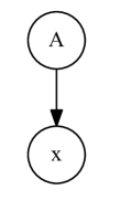
Figure 1. The derivation tree of the height $h=1$ for the string $x=l(\pi)$.

Inductive step: Assume that the statement of the lemma holds for any $k\leq(p-1)$ and show that it also holds for $k=p$ where $p\geq 2$. For any $i,j$ and for any non-terminal $A\in N$,

$$A\in a^{(p)}_{i,j}\text{ iff }A\in a^{(p-1)}_{i,j}\text{ or }A\in(a^{(p-1)}\times a^{(p-1)})_{i,j},$$

since

$$a^{(p)}=a^{(p-1)}\cup(a^{(p-1)}\times a^{(p-1)}).$$

Let $A\in a^{(p-1)}_{i,j}$. By the inductive hypothesis, $A\in a^{(p-1)}_{i,j}$ iff $(i,j)\in R_{A}$ and there exists $i\pi j$, such that there is a derivation tree of the height $h\leq(p-1)$ for the string $l(\pi)$ and a context-free grammar $G_{A}=(N,\Sigma,P,A)$. The statement of the lemma holds for $k=p$ since the height $h$ of this tree is also less than or equal to $p$.

Let $A\in(a^{(p-1)}\times a^{(p-1)})_{i,j}$. By the definition of the binary operation $(\cdot)$ on arbitrary subsets, $A\in(a^{(p-1)}\times a^{(p-1)})_{i,j}$ iff there are $r$, $B\in a^{(p-1)}_{i,r}$ and $C\in a^{(p-1)}_{r,j}$, such that $(A\rightarrow BC)\in P$. Hence, by the inductive hypothesis, there are $i\pi_{1}r$ and $r\pi_{2}j$, such that $(i,r)\in R_{B}$ and $(r,j)\in R_{C}$, and there are the derivation trees $T_{B}$ and $T_{C}$ of heights $h_{1}\leq(p-1)$ and $h_{2}\leq(p-1)$ for the strings $w_{1}=l(\pi_{1})$, $w_{2}=l(\pi_{2})$ and the context-free grammars $G_{B}$, $G_{C}$ respectively. Thus, the concatenation of paths $\pi_{1}$ and $\pi_{2}$ is $i\pi j$, where $(i,j)\in R_{A}$ and there is a derivation tree of the height $h=1+max(h_{1},h_{2})$, shown in Figure 2, for the string $w=l(\pi)$ and a context-free grammar $G_{A}$.

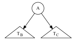
Figure 2. The derivation tree of the height $h=1+max(h_{1},h_{2})$ for the string $w=l(\pi)$, where $T_{B}$ and $T_{C}$ are the derivation trees for strings $w_{1}$ and $w_{2}$ respectively.

The statement of the lemma holds for $k=p$ since the height $h=1+max(h_{1},h_{2})\leq p$. This completes the proof of the lemma. ∎

Theorem 2.

Let $D=(V,E)$ be a graph and let $G=(N,\Sigma,P)$ be a grammar. Then for any $i,j$ and for any non-terminal $A\in N$, $A\in a^{cf}_{i,j}$ iff $(i,j)\in R_{A}$.

Proof.

Since the matrix $a^{cf}=a^{(1)}\cup a^{(2)}\cup\cdots,$ for any $i,j$ and for any non-terminal $A\in N$, $A\in a^{cf}_{i,j}$ iff there is $k\geq 1$, such that $A\in a^{(k)}_{i,j}$. By the lemma 4.1, $A\in a^{(k)}_{i,j}$ iff $(i,j)\in R_{A}$ and there is $i\pi j$, such that there is a derivation tree of the height $h\leq k$ for the string $l(\pi)$ and a context-free grammar $G_{A}=(N,\Sigma,P,A)$. This completes the proof of the theorem. ∎

We can, therefore, determine whether $(i,j)\in R_{A}$ by asking whether $A\in a^{cf}_{i,j}$. Thus, we show how the context-free relations $R_{A}$ can be calculated by computing the transitive closure $a^{cf}$ of the matrix $a$.

4.2. The algorithm

In this section, we introduce an algorithm for calculating the transitive closure $a^{cf}$ which was discussed in Section 4.1.

Let $D=(V,E)$ be the input graph and $G=(N,\Sigma,P)$ be the input grammar.

1:function contextFreePathQuerying(D, G)

2:  $n\leftarrow$ the number of nodes in $D$

3:  $E\leftarrow$ the directed edge-relation from $D$

4:  $P\leftarrow$ the set of production rules in $G$

5:  $T\leftarrow$ the matrix $n\times n$ in which each element is $\varnothing$

6:  for all $(i,x,j)\in E$ do $\triangleright$ Matrix initialization

7:   $T_{i,j}\leftarrow T_{i,j}\cup\{A~{}|~{}(A\rightarrow x)\in P\}$   

8:  while matrix $T$ is changing do

9:   $T\leftarrow T\cup(T\times T)$ $\triangleright$ Transitive closure $T^{cf}$ calculation   

10:  return $T$

Algorithm 1 Context-free recognizer for graphs

Note that the matrix initialization in lines 6-7 of the Algorithm 1 can handle arbitrary graph $D$. For example, if a graph $D$ contains multiple edges $(i,x_{1},j)$ and $(i,x_{2},j)$ then both the elements of the set $\{A~{}|~{}(A\rightarrow x_{1})\in P\}$ and the elements of the set $\{A~{}|~{}(A\rightarrow x_{2})\in P\}$ will be added to $T_{i,j}$.

We need to show that the Algorithm 1 terminates in a finite number of steps. Since each element of the matrix $T$ contains no more than $|N|$ non-terminals, the total number of non-terminals in the matrix $T$ does not exceed $|V|^{2}|N|$. Therefore, the following theorem holds.

Theorem 3.

Let $D=(V,E)$ be a graph and let $G=(N,\Sigma,P)$ be a grammar. The Algorithm 1 terminates in a finite number of steps.

Proof.

It is sufficient to show, that the operation in the line 9 of the Algorithm 1 changes the matrix $T$ only finite number of times. Since this operation can only add non-terminals to some elements of the matrix $T$, but not remove them, it can change the matrix $T$ no more than $|V|^{2}|N|$ times. ∎

Denote the number of elementary operations executed by the algorithm of multiplying two $n\times n$ Boolean matrices as $BMM(n)$. According to Valiant, the matrix multiplication operation in the line 9 of the Algorithm 1 can be calculated in $O(|N|^{2}BMM(|V|))$. Denote the number of elementary operations executed by the matrix union operation of two $n\times n$ Boolean matrices as $BMU(n)$. Similarly, it can be shown that the matrix union operation in the line 9 of the Algorithm 1 can be calculated in $O(|N|^{2}BMU(n))$. Since the line 9 of the Algorithm 1 is executed no more than $|V|^{2}|N|$ times, the following theorem holds.

Theorem 4.

Let $D=(V,E)$ be a graph and let $G=(N,\Sigma,P)$ be a grammar. The Algorithm 1 calculates the transitive closure $T^{cf}$ in $O(|V|^{2}|N|^{3}(BMM(|V|)+BMU(|V|)))$.

4.3. An example

In this section, we provide a step-by-step demonstration of the proposed algorithm. For this, we consider the classical same-generation query (Abiteboul et al., 1995).

The example query is based on the context-free grammar $G=(N,\Sigma,P)$ where:

• The set of non-terminals $N=\{S\}$.

• The set of terminals

  $$\Sigma=\{subClassOf,subClassOf^{-1},type,type^{-1}\}.$$

• The set of production rules $P$ is presented in Figure 3.

$$\begin{array}[]{rccl}0:&S&\rightarrow&\text{{subClassOf}}^{-1}\ S\ \text{{subClassOf}}\\ 1:&S&\rightarrow&\text{{type}}^{-1}\ S\ \text{{type}}\\ 2:&S&\rightarrow&\text{{subClassOf}}^{-1}\ \text{{subClassOf}}\\ 3:&S&\rightarrow&\text{{type}}^{-1}\ \text{{type}}\\ \end{array}$$

Figure 3. Production rules for the example query grammar.

Since the proposed algorithm processes only grammars in Chomsky normal form, we first transform the grammar $G$ into an equivalent grammar $G^{\prime}=(N^{\prime},\Sigma^{\prime},P^{\prime})$ in normal form, where:

• The set of non-terminals $N^{\prime}=\{S,S_{1},S_{2},S_{3},S_{4},S_{5},S_{6}\}$.

• The set of terminals

  $$\Sigma^{\prime}=\{subClassOf,subClassOf^{-1},type,type^{-1}\}.$$

• The set of production rules $P^{\prime}$ is presented in Figure 4.

$$\begin{array}[]{rccl}0:&S&\rightarrow&S_{1}\ S_{5}\\ 1:&S&\rightarrow&S_{3}\ S_{6}\\ 2:&S&\rightarrow&S_{1}\ S_{2}\\ 3:&S&\rightarrow&S_{3}\ S_{4}\\ 4:&S_{5}&\rightarrow&S\ S_{2}\\ 5:&S_{6}&\rightarrow&S\ S_{4}\\ 6:&S_{1}&\rightarrow&\text{{subClassOf}}^{-1}\\ 7:&S_{2}&\rightarrow&\text{{subClassOf}}\\ 8:&S_{3}&\rightarrow&\text{{type}}^{-1}\\ 9:&S_{4}&\rightarrow&\text{{type}}\\ \end{array}$$

Figure 4. Production rules for the example query grammar in normal form.

We run the query on a graph presented in Figure 5.

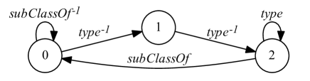
Figure 5. An input graph for the example query.

We provide a step-by-step demonstration of the work with the given graph $D$ and grammar $G^{\prime}$ of the Algorithm 1. After the matrix initialization in lines 6-7 of the Algorithm 1, we have a matrix $T_{0}$ presented in Figure 6.

$$T_{0}=\begin{pmatrix}\{S_{1}\}&\{S_{3}\}&\varnothing\\ \varnothing&\varnothing&\{S_{3}\}\\ \{S_{2}\}&\varnothing&\{S_{4}\}\end{pmatrix}$$

Figure 6. The initial matrix for the example query.

Let $T_{i}$ be the matrix $T$ obtained after executing the loop in lines 8-9 of the Algorithm 1 $i$ times. The calculation of the matrix $T_{1}$ is shown in Figure 7.

$$T_{0}\times T_{0}=\begin{pmatrix}\varnothing&\varnothing&\varnothing\\ \varnothing&\varnothing&\{S\}\\ \varnothing&\varnothing&\varnothing\end{pmatrix}$$

$$T_{1}=T_{0}\cup(T_{0}\times T_{0})=\begin{pmatrix}\{S_{1}\}&\{S_{3}\}&\varnothing\\ \varnothing&\varnothing&\{S_{3},S\}\\ \{S_{2}\}&\varnothing&\{S_{4}\}\end{pmatrix}$$

Figure 7. The first iteration of computing the transitive closure for the example query.

When the algorithm at some iteration finds new paths in the graph $D$, then it adds corresponding nonterminals to the matrix $T$. For example, after the first loop iteration, non-terminal $S$ is added to the matrix $T$. This non-terminal is added to the element with a row index $i=1$ and a column index $j=2$. This means that there is $i\pi j$ (a path $\pi$ from the node 1 to the node 2), such that $S\xrightarrow{*}l(\pi)$. For example, such a path consists of two edges with labels $type^{-1}$ and $type$, and thus $S\xrightarrow{*}type^{-1}\ type$.

The calculation of the transitive closure is completed after $k$ iterations when a fixpoint is reached: $T_{k-1}=T_{k}$. For the example query, $k=6$ since $T_{6}=T_{5}$. The remaining iterations of computing the transitive closure are presented in Figure 8.

$$T_{2}=\begin{pmatrix}\{S_{1}\}&\{S_{3}\}&\varnothing\\ \{S_{5}\}&\varnothing&\{S_{3},S,S_{6}\}\\ \{S_{2}\}&\varnothing&\{S_{4}\}\end{pmatrix}$$

$$T_{3}=\begin{pmatrix}\{S_{1}\}&\{S_{3}\}&\{S\}\\ \{S_{5}\}&\varnothing&\{S_{3},S,S_{6}\}\\ \{S_{2}\}&\varnothing&\{S_{4}\}\end{pmatrix}$$

$$T_{4}=\begin{pmatrix}\{S_{1},S_{5}\}&\{S_{3}\}&\{S,S_{6}\}\\ \{S_{5}\}&\varnothing&\{S_{3},S,S_{6}\}\\ \{S_{2}\}&\varnothing&\{S_{4}\}\end{pmatrix}$$

$$T_{5}=\begin{pmatrix}\{S_{1},S_{5},S\}&\{S_{3}\}&\{S,S_{6}\}\\ \{S_{5}\}&\varnothing&\{S_{3},S,S_{6}\}\\ \{S_{2}\}&\varnothing&\{S_{4}\}\end{pmatrix}$$

Figure 8. Remaining states of the matrix $T$.

Thus, the result of the Algorithm 1 for the example query is the matrix $T_{5}=T_{6}$. Now, after constructing the transitive closure, we can construct the context-free relations $R_{A}$. These relations for each non-terminal of the grammar $G^{\prime}$ are presented in Figure 9.

$$R_{S} = \{(0,0),(0,2),(1,2)\},$$

$$R_{S_{1}} = \{(0,0)\},$$

$$R_{S_{2}} = \{(2,0)\},$$

$$R_{S_{3}} = \{(0,1),(1,2)\},$$

$$R_{S_{4}} = \{(2,2)\},$$

$$R_{S_{5}} = \{(0,0),(1,0)\},$$

$$R_{S_{6}} = \{(0,2),(1,2)\}.$$

Figure 9. Context-free relations for the example query.

By the context-free relation $R_{S}$, we can conclude that there are paths in a graph $D$ only from the node 0 to the node 0, from the node 0 to the node 2 or from the node 1 to the node 2, corresponding to the context-free grammar $G_{S}$. This conclusion is based on the fact that a grammar $G^{\prime}_{S}$ is equivalent to the grammar $G_{S}$ and $L(G_{S})=L(G_{S}^{\prime})$.

5. Context-free path querying using single-path semantics

In this section, we show how the context-free path query evaluation using the single-path query semantics can be reduced to the calculation of matrix transitive closure $a^{cf}$ and prove the correctness of this reduction.

At the first step, we show how the calculation of matrix transitive closure $a^{cf}$ which was discussed in Section 4.1 can be modified to compute the length of some path $i\pi j$ for all $(i,j)\in R_{A}$, such that $A\xrightarrow{*}l(\pi)$. This is sufficient to solve the problem of context-free path query evaluation using the single-path query semantics since the required path of a fixed length from the node $i$ to the node $j$ can be found by a simple search and checking whether the labels of this path form a string which can be derived from a non-terminal $A$.

Let $G=(N,\Sigma,P)$ be a grammar and $D=(V,E)$ be a graph. We enumerate the nodes of the graph $D$ from 0 to $(|V|-1)$. We initialize the $|V|\times|V|$ matrix $a$ with $\varnothing$. We associate each non-terminal in matrix $a$ with the corresponding path length. For convenience, each nonterminal $A$ in the $a_{i,j}$ is represented as a pair $(A,k)$ where $k$ is an associated path length. For every $i$ and $j$ we set

$$a_{i,j}=\{(A_{k},1)~{}|~{}((i,x,j)\in E)\wedge((A_{k}\rightarrow x)\in P)\}$$

since initially all path lengths are equal to $1$. Finally, we compute the transitive closure $a^{cf}$ and if non-terminal $A$ is added to $a^{(p)}_{i,j}$ by using the production rule $(A\rightarrow BC)\in P$ where $(B,l_{B})\in a^{(p-1)}_{i,k}$, $(C,l_{C})\in a^{(p-1)}_{k,j}$, then the path length $l_{A}$ associated with non-terminal $A$ is calculated as $l_{A}=l_{B}+l_{C}$. Therefore $(A,l_{A})\in a^{(p)}_{i,j}$. Note that if some non-terminal $A$ with an associated path length $l_{1}$ is in $a^{(p)}_{i,j}$, then the non-terminal $A$ is not added to the $a^{(k)}_{i,j}$ with an associated path length $l_{2}$ for all $l_{2}\neq l_{1}$ and $k\geq p$. For the transitive closure $a^{cf}$, the following statements hold.

Lemma 5.1.

Let $D=(V,E)$ be a graph, let $G=(N,\Sigma,P)$ be a grammar. Then for any $i,j$ and for any non-terminal $A\in N$, if $(A,l_{A})\in a^{(k)}_{i,j}$, then there is $i\pi j$, such that $A\xrightarrow{*}l(\pi)$ and the length of $\pi$ is equal to $l_{A}$.

Proof.

(Proof by Induction)

Basis: Show that the statement of the lemma holds for $k=1$. For any $i,j$ and for any non-terminal $A\in N$, $(A,l_{A})\in a^{(1)}_{i,j}$ iff $l_{A}=1$ and there is $i\pi j$ that consists of a unique edge $e$ from the node $i$ to the node $j$ and $(A\rightarrow x)\in P$ where $x=l(\pi)$. Therefore there is $i\pi j$, such that $A\xrightarrow{*}l(\pi)$ and the length of $\pi$ is equal to $l_{A}$. Thus, it has been shown that the statement of the lemma holds for $k=1$.

Inductive step: Assume that the statement of the lemma holds for any $k\leq(p-1)$ and show that it also holds for $k=p$ where $p\geq 2$. For any $i,j$ and for any non-terminal $A\in N$, $(A,l_{A})\in a^{(p)}_{i,j}$ iff $(A,l_{A})\in a^{(p-1)}_{i,j}$ or $(A,l_{A})\in(a^{(p-1)}\times a^{(p-1)})_{i,j}$ since $a^{(p)}=a^{(p-1)}\cup(a^{(p-1)}\times a^{(p-1)}).$

Let $(A,l_{A})\in a^{(p-1)}_{i,j}$. By the inductive hypothesis, there is $i\pi j$, such that $A\xrightarrow{*}l(\pi)$ and the length of $\pi$ is equal to $l_{A}$. Therefore the statement of the lemma holds for $k=p$.

Let $(A,l_{A})\in(a^{(p-1)}\times a^{(p-1)})_{i,j}$. By the definition, $(A,l_{A})\in(a^{(p-1)}\times a^{(p-1)})_{i,j}$ iff there are $r$, $(B,l_{B})\in a^{(p-1)}_{i,r}$ and $(C,l_{C})\in a^{(p-1)}_{r,j}$, such that $(A\rightarrow BC)\in P$ and $l_{A}=l_{B}+l_{C}$. Hence, by the inductive hypothesis, there are $i\pi_{1}r$ and $r\pi_{2}j$, such that

$$(B\xrightarrow{*}l(\pi_{1}))\wedge(C\xrightarrow{*}l(\pi_{2})),$$

where the length of $\pi_{1}$ is equal to $l_{B}$ and the length of $\pi_{2}$ is equal to $l_{C}$. Thus, the concatenation of paths $\pi_{1}$ and $\pi_{2}$ is $i\pi j$, where $A\xrightarrow{*}l(\pi)$ and the length of $\pi$ is equal to $l_{A}$. Therefore the statement of the lemma holds for $k=p$ and this completes the proof of the lemma. ∎

Theorem 5.

Let $D=(V,E)$ be a graph and let $G=(N,\Sigma,P)$ be a grammar. Then for any $i,j$ and for any non-terminal $A\in N$, if $(A,l_{A})\in a^{cf}_{i,j}$, then there is $i\pi j$, such that $A\xrightarrow{*}l(\pi)$ and the length of $\pi$ is equal to $l_{A}$.

Proof.

Since the matrix $a^{cf}=a^{(1)}\cup a^{(2)}\cup\cdots$, for any $i,j$ and for any non-terminal $A\in N$, if $(A,l_{A})\in a^{cf}_{i,j}$, then there is $k\geq 1$, such that $A\in a^{(k)}_{i,j}$. By the lemma 5.1, if $(A,l_{A})\in a^{(k)}_{i,j}$, then there is $i\pi j$, such that $A\xrightarrow{*}l(\pi)$ and the length of $\pi$ is equal to $l_{A}$. This completes the proof of the theorem. ∎

By the theorem 2, we can determine whether $(i,j)\in R_{A}$ by asking whether $(A,l_{A})\in a^{cf}_{i,j}$ for some $l_{A}$. By the theorem 5, there is $i\pi j$, such that $A\xrightarrow{*}l(\pi)$ and the length of $\pi$ is equal to $l_{A}$. Therefore, we can find such a path $\pi$ of the length $l_{A}$ from the node $i$ to the node $j$ by a simple search. Thus, we show how the context-free path query evaluation using the single-path query semantics can be reduced to the calculation of matrix transitive closure $a^{cf}$. Note that the time complexity of the algorithm for context-free path querying w.r.t. the single-path semantics no longer depends on the Boolean matrix multiplications since we modify the matrix representation and operations on the matrix elements.

6. Evaluation

In this paper, we do not estimate the practical value of the algorithm for the context-free path querying w.r.t. the single-path query semantics, since this algorithm depends significant on the implementation of the path searching. To show the practical applicability of the algorithm for context-free path querying w.r.t. the relational query semantics, we implement this algorithm using a variety of optimizations and apply these implementations to the navigation query problem for a dataset of popular ontologies taken from (Zhang et al., 2016). We also compare the performance of our implementations with existing analogs from (Grigorev and Ragozina, 2016; Zhang et al., 2016). These analogs use more complex algorithms, while our algorithm uses only simple matrix operations.

Since our algorithm works with graphs, each RDF file from a dataset was converted to an edge-labeled directed graph as follows. For each triple $(o,p,s)$ from an RDF file, we added edges $(o,p,s)$ and $(s,p^{-1},o)$ to the graph. We also constructed synthetic graphs $g_{1}$, $g_{2}$ and $g_{3}$, simply repeating the existing graphs.

All tests were run on a PC with the following characteristics:

• OS: Microsoft Windows 10 Pro

• System Type: x64-based PC

• CPU: Intel(R) Core(TM) i7-4790 CPU @ 3.60GHz, 3601 Mhz, 4 Core(s), 4 Logical Processor(s)

• RAM: 16 GB

• GPU: NVIDIA GeForce GTX 1070

  • CUDA Cores: 1920

  • Core clock: 1556 MHz

  • Memory data rate: 8008 MHz

  • Memory interface: 256-bit

  • Memory bandwidth: 256.26 GB/s

  • Dedicated video memory: 8192 MB GDDR5

We denote the implementation of the algorithm from a paper (Grigorev and Ragozina, 2016) as $GLL$. The algorithm presented in this paper is implemented in F# programming language (Syme et al., 2012) and is available on GitHub. We denote our implementations of the proposed algorithm as follows:

• dGPU (dense GPU) — an implementation using row-major order for general matrix representation and a GPU for matrix operations calculation. For calculations of matrix operations on a GPU, we use a wrapper for the CUBLAS library from the managedCuda library.

• sCPU (sparse CPU) — an implementation using CSR format for sparse matrix representation and a CPU for matrix operations calculation. For sparse matrix representation in CSR format, we use the Math.Net Numerics package.

• sGPU (sparse GPU) — an implementation using the CSR format for sparse matrix representation and a GPU for matrix operations calculation. For calculations of the matrix operations on a GPU, where matrices represented in a CSR format, we use a wrapper for the CUSPARSE library from the managedCuda library.

We omit $dGPU$ performance on graphs $g_{1}$, $g_{2}$ and $g_{3}$ since a dense matrix representation leads to a significant performance degradation with the graph size growth.

We evaluate two classical same-generation queries (Abiteboul et al., 1995) which, for example, are applicable in bioinformatics.

Query 1 is based on the grammar $G^{1}_{S}$ for retrieving concepts on the same layer, where:

• The grammar $G^{1}=(N^{1},\Sigma^{1},P^{1})$.

• The set of non-terminals $N^{1}=\{S\}$.

• The set of terminals

  $$\Sigma^{1}=\{subClassOf,subClassOf^{-1},type,type^{-1}\}.$$

• The set of production rules $P^{1}$ is presented in Figure 10.

$$\begin{array}[]{rccl}0:&S&\rightarrow&\text{{subClassOf}}^{-1}\ S\ \text{{subClassOf}}\\ 1:&S&\rightarrow&\text{{type}}^{-1}\ S\ \text{{type}}\\ 2:&S&\rightarrow&\text{{subClassOf}}^{-1}\ \text{{subClassOf}}\\ 3:&S&\rightarrow&\text{{type}}^{-1}\ \text{{type}}\\ \end{array}$$

Figure 10. Production rules for the query 1 grammar.

Table 1. Evaluation results for Query 1

Ontology	#triples	#results	GLL(ms)	dGPU(ms)	sCPU(ms)	sGPU(ms)
skos	252	810	10	56	14	12
generations	273	2164	19	62	20	13
travel	277	2499	24	69	22	30
univ-bench	293	2540	25	81	25	15
atom-primitive	425	15454	255	190	92	22
biomedical-measure-primitive	459	15156	261	266	113	20
foaf	631	4118	39	154	48	9
people-pets	640	9472	89	392	142	32
funding	1086	17634	212	1410	447	36
wine	1839	66572	819	2047	797	54
pizza	1980	56195	697	1104	430	24
$g_{1}$	8688	141072	1926	—	26957	82
$g_{2}$	14712	532576	6246	—	46809	185
$g_{3}$	15840	449560	7014	—	24967	127

Table 2. Evaluation results for Query 2

Ontology	#triples	#results	GLL(ms)	dGPU(ms)	sCPU(ms)	sGPU(ms)
skos	252	1	1	10	2	1
generations	273	0	1	9	2	0
travel	277	63	1	31	7	10
univ-bench	293	81	11	55	15	9
atom-primitive	425	122	66	36	9	2
biomedical-measure-primitive	459	2871	45	276	91	24
foaf	631	10	2	53	14	3
people-pets	640	37	3	144	38	6
funding	1086	1158	23	1246	344	27
wine	1839	133	8	722	179	6
pizza	1980	1262	29	943	258	23
$g_{1}$	8688	9264	167	—	21115	38
$g_{2}$	14712	1064	46	—	10874	21
$g_{3}$	15840	10096	393	—	15736	40

The grammar $G^{1}$ is transformed into an equivalent grammar in normal form, which is necessary for our algorithm. This transformation is the same as in Section 4.3. Let $R_{S}$ be a context-free relation for a start non-terminal in the transformed grammar.

The result of query 1 evaluation is presented in Table 1, where #triples is a number of triples $(o,p,s)$ in an RDF file, and #results is a number of pairs $(n,m)$ in the context-free relation $R_{S}$. We can determine whether $(i,j)\in R_{S}$ by asking whether $S\in a^{cf}_{i,j}$, where $a^{cf}$ is a transitive closure calculated by the proposed algorithm. All implementations in Table 1 have the same #results and demonstrate up to 1000 times better performance as compared to the algorithm presented in (Zhang et al., 2016) for $Q_{1}$. Our implementation $sGPU$ demonstrates a better performance than $GLL$. We also can conclude that acceleration from the $GPU$ increases with the graph size growth.

Query 2 is based on the grammar $G^{2}_{S}$ for retrieving concepts on the adjacent layers, where:

• The grammar $G^{2}=(N^{2},\Sigma^{2},P^{2})$.

• The set of non-terminals $N^{2}=\{S,B\}$.

• The set of terminals

  $$\Sigma^{2}=\{subClassOf,subClassOf^{-1}\}.$$

• The set of production rules $P^{2}$ is presented in Figure 11.

$$\begin{array}[]{rccl}0:&S&\rightarrow&B\ \text{{subClassOf}}\\ 1:&S&\rightarrow&\text{{subClassOf}}\\ 2:&B&\rightarrow&\text{{subClassOf}}^{-1}\ B\ \text{{subClassOf}}\\ 3:&B&\rightarrow&\text{{subClassOf}}^{-1}\ \text{{subClassOf}}\\ \end{array}$$

Figure 11. Production rules for the query 2 grammar.

The grammar $G^{2}$ is transformed into an equivalent grammar in normal form. Let $R_{S}$ be a context-free relation for a start non-terminal in the transformed grammar.

The result of the query 2 evaluation is presented in Table 2. All implementations in Table 2 have the same #results. On almost all graphs $sGPU$ demonstrates a better performance than $GLL$ implementation and we also can conclude that acceleration from the $GPU$ increases with the graph size growth.

As a result, we conclude that our algorithm can be applied to some real-world problems and it allows us to speed up computations by means of GPGPU.

7. Conclusion and future work

In this paper, we have shown how the context-free path query evaluation w.r.t. the relational and the single-path query semantics can be reduced to the calculation of matrix transitive closure. Also, we provided a formal proof of the correctness of the proposed reduction. In addition, we introduced an algorithm for computing this transitive closure, which allows us to efficiently apply GPGPU computing techniques. Finally, we have shown the practical applicability of the proposed algorithm by running different implementations of our algorithm on real-world data.

We can identify several open problems for further research. In this paper, we have considered only two semantics of context-free path querying but there are other important semantics, such as all-path query semantics (Hellings, 2015) which requires presenting all paths for all triples $(A,m,n)$. Context-free path querying implemented with the algorithm (Grigorev and Ragozina, 2016) can answer the queries in the all-path query semantics by constructing a parse forest. It is possible to construct a parse forest for a linear input by matrix multiplication (Okhotin, 2014). Whether it is possible to generalize this approach for a graph input is an open question.

In our algorithm, we calculate the matrix transitive closure naively, but there are algorithms for the transitive closure calculation, which are asymptotically more efficient. Therefore, the question is whether it is possible to apply these algorithms for the matrix transitive closure calculation to the problem of context-free path querying.

Also, there are conjunctive (Okhotin, 2013) and Boolean grammars (Okhotin, 2004), which have more expressive power than context-free grammars. Conjunctive language and Boolean path querying problems are undecidable (Hellings, 2014) but our algorithm can be trivially generalized to work on this grammars because parsing with conjunctive and Boolean grammars can be expressed by matrix multiplication (Okhotin, 2014). It is not clear what a result of our algorithm applied to this grammars would look like. Our hypothesis is that it would produce the upper approximation of a solution. Also, path querying problem w.r.t. the conjunctive grammars can be applied to static code analysis (Zhang and Su, 2017).

From a practical point of view, matrix multiplication in the main loop of the proposed algorithm may be performed on different GPGPU independently. It can help to utilize the power of multi-GPU systems and increase the performance of the context-free path querying.

There is an algorithm (Katz and Kider Jr, 2008) for transitive closure calculation on directed graphs which generalized to handle graph sizes inherently larger than the DRAM memory available on the GPU. Therefore, the question is whether it is possible to apply this approach to the matrix transitive closure calculation in the problem of context-free path querying.

References

- (1)
- Abiteboul et al. (1995) Serge Abiteboul, Richard Hull, and Victor Vianu. 1995. Foundations of databases: the logical level. Addison-Wesley Longman Publishing Co., Inc.
- Abiteboul and Vianu (1997) Serge Abiteboul and Victor Vianu. 1997. Regular path queries with constraints. In Proceedings of the sixteenth ACM SIGACT-SIGMOD-SIGART symposium on Principles of database systems. ACM, 122–133.
- Anderson et al. (2013) James WJ Anderson, Ádám Novák, Zsuzsanna Sükösd, Michael Golden, Preeti Arunapuram, Ingolfur Edvardsson, and Jotun Hein. 2013. Quantifying variances in comparative RNA secondary structure prediction. BMC bioinformatics 14, 1 (2013), 149.
- Barrett et al. (2000) Chris Barrett, Riko Jacob, and Madhav Marathe. 2000. Formal-language-constrained path problems. SIAM J. Comput. 30, 3 (2000), 809–837.
- Bastani et al. (2015) Osbert Bastani, Saswat Anand, and Alex Aiken. 2015. Specification inference using context-free language reachability. In ACM SIGPLAN Notices, Vol. 50. ACM, 553–566.
- Che et al. (2016) Shuai Che, Bradford M Beckmann, and Steven K Reinhardt. 2016. Programming GPGPU Graph Applications with Linear Algebra Building Blocks. International Journal of Parallel Programming (2016), 1–23.
- Chomsky (1959) Noam Chomsky. 1959. On certain formal properties of grammars. Information and control 2, 2 (1959), 137–167.
- Fan et al. (2011) Wenfei Fan, Jianzhong Li, Shuai Ma, Nan Tang, and Yinghui Wu. 2011. Adding regular expressions to graph reachability and pattern queries. In Data Engineering (ICDE), 2011 IEEE 27th International Conference on. IEEE, 39–50.
- Grigorev and Ragozina (2016) Semyon Grigorev and Anastasiya Ragozina. 2016. Context-Free Path Querying with Structural Representation of Result. arXiv preprint arXiv:1612.08872 (2016).
- Grune and Jacobs (2006) Dick Grune and Ceriel J. H. Jacobs. 2006. Parsing Techniques (Monographs in Computer Science). Springer-Verlag New York, Inc., Secaucus, NJ, USA.
- Hellings (2014) J. Hellings. 2014. Conjunctive context-free path queries. (2014).
- Hellings (2015) Jelle Hellings. 2015. Querying for Paths in Graphs using Context-Free Path Queries. arXiv preprint arXiv:1502.02242 (2015).
- Kasami (1965) Tadao Kasami. 1965. AN EFFICIENT RECOGNITION AND SYNTAXANALYSIS ALGORITHM FOR CONTEXT-FREE LANGUAGES. Technical Report. DTIC Document.
- Katz and Kider Jr (2008) Gary J Katz and Joseph T Kider Jr. 2008. All-pairs shortest-paths for large graphs on the GPU. In Proceedings of the 23rd ACM SIGGRAPH/EUROGRAPHICS symposium on Graphics hardware. Eurographics Association, 47–55.
- Mendelzon and Wood (1995) A. Mendelzon and P. Wood. 1995. Finding Regular Simple Paths in Graph Databases. SIAM J. Computing 24, 6 (1995), 1235–1258.
- Nolé and Sartiani (2016) Maurizio Nolé and Carlo Sartiani. 2016. Regular path queries on massive graphs. In Proceedings of the 28th International Conference on Scientific and Statistical Database Management. ACM, 13.
- Okhotin (2004) Alexander Okhotin. 2004. Boolean grammars. Information and Computation 194, 1 (2004), 19–48.
- Okhotin (2013) Alexander Okhotin. 2013. Conjunctive and Boolean grammars: the true general case of the context-free grammars. Computer Science Review 9 (2013), 27–59.
- Okhotin (2014) Alexander Okhotin. 2014. Parsing by matrix multiplication generalized to Boolean grammars. Theoretical Computer Science 516 (2014), 101–120.
- Reps (1998) Thomas Reps. 1998. Program analysis via graph reachability. Information and software technology 40, 11 (1998), 701–726.
- Reutter et al. (2017) Juan L Reutter, Miguel Romero, and Moshe Y Vardi. 2017. Regular queries on graph databases. Theory of Computing Systems 61, 1 (2017), 31–83.
- Scott and Johnstone (2010) Elizabeth Scott and Adrian Johnstone. 2010. GLL parsing. Electronic Notes in Theoretical Computer Science 253, 7 (2010), 177–189.
- Sevon and Eronen (2008) Petteri Sevon and Lauri Eronen. 2008. Subgraph queries by context-free grammars. Journal of Integrative Bioinformatics 5, 2 (2008), 100.
- Syme et al. (2012) Don Syme, Adam Granicz, and Antonio Cisternino. 2012. Expert F# 3.0. Springer.
- Valiant (1975) Leslie G Valiant. 1975. General context-free recognition in less than cubic time. Journal of computer and system sciences 10, 2 (1975), 308–315.
- Xu et al. (2009) Guoqing Xu, Atanas Rountev, and Manu Sridharan. 2009. Scaling CFL-reachability-based points-to analysis using context-sensitive must-not-alias analysis. In ECOOP, Vol. 9. Springer, 98–122.
- Yannakakis (1990) Mihalis Yannakakis. 1990. Graph-theoretic methods in database theory. In Proceedings of the ninth ACM SIGACT-SIGMOD-SIGART symposium on Principles of database systems. ACM, 230–242.
- Younger (1967) Daniel H Younger. 1967. Recognition and parsing of context-free languages in time n3. Information and control 10, 2 (1967), 189–208.
- Zhang and Su (2017) Qirun Zhang and Zhendong Su. 2017. Context-sensitive data-dependence analysis via linear conjunctive language reachability. In Proceedings of the 44th ACM SIGPLAN Symposium on Principles of Programming Languages. ACM, 344–358.
- Zhang et al. (2016) X. Zhang, Z. Feng, X. Wang, G. Rao, and W. Wu. 2016. Context-free path queries on RDF graphs. In International Semantic Web Conference. Springer, 632–648.