ACCUMULATION OF INDIVIDUAL FITNESS OR WEALTH AS A POPULATION GAME

Abstract

The accumulation of individual fitness or wealth is modelled as a population game in which pairs of individuals are recurrently and randomly matched to play a game over a resource. In addition, all individuals have random access to a constant background resource, and their fitness or wealth depreciates over time. For brevity we focus on the well-known Hawk-Dove game. In the base-line model, the probability of winning a fight (that is, when both play Hawk) is the same for both parties. In an extended version, the individual with higher current fitness or wealth has a higher probability of winning. Analytical results are given for the fitness/wealth distribution at any given time, for the evolution of average fitness/wealth over time, and for the asymptotics with respect to time and population size. Long-run average fitness/wealth is non-monotonic in the value of the resource, thus providing a potential explanation of the curse of the riches.

Keywords: Hawk-Dove, fitness dynamics, wealth dynamics, fitness distribution, wealth distribution, curse of the riches, ergodicity, propagation of chaos.

1 Introduction

This paper analyzes the accumulation and depreciation of personal fitness or wealth in a finite population where individuals are recurrently and randomly paired to interact with each other. The interaction takes the form of a symmetric two-player game over some resource, and the payoffs, representing gains and losses, are added to and subtracted from the two individuals’ current levels of fitness or wealth. For the sake of definiteness and brevity, we focus on a simple but canonical Hawk-Dove game. However, the machinery applies to any symmetric finite game, and can readily be extended to arbitrary finite games. We generalize a deterministic mean-field model sketched in Weibull (1999). To the best of our knowledge, the present study is the first analysis of the stochastic accumulation and depreciation of individual and average fitness or wealth in populations of strategically interacting individuals. As will be seen, inequality arises over time even if all individuals are ex ante identical and start out from the same level of fitness or wealth.

The Hawk-Dove game was used by Maynard Smith and Price (1973) as an illustration of the possibility that a mixed strategy may be evolutionarily stable. While they only considered expected payoffs, we here consider realized payoffs. In particular, if both players use the Hawk strategy, a fight results in which the winner takes all and the loser incurs a loss. Consequently, their individual levels of fitness or wealth diverge after such an interaction. In our base-line model, we follow Maynard Smith and Price in assuming that all individuals have the same chance of winning a fight. In an extended version, the more fit or wealthier individual has a higher chances of winning a fight.

The main focus of this study is on the induced stochastic population dynamics. While the individuals in our model may be animals or other biological organisms, and payoffs may be interpreted as increments to personal fitness, as in Maynard-Smith’s and Price’s original contribution, we subsequently interpret the model only in terms of personal wealth, where the game represent economic opportunities for production or trade, opportunities that spontaneously arise for given natural resources and institutions. Whenever such an interaction opportunity arises, each of the two parties may seek cooperation (play "Dove") or conflict (play "Hawk"). If both seek cooperation, they split the resource equally. If both seek conflict, one of them wins the resource and the other individual incurs a loss. If one individual seeks cooperation and the other conflict, the latter obtains the full value of the resource and the former neither has a gain or loss. This is but one example of games that may be used to represent economic activity in the present framework.

In addition to the game payoffs, individuals now and then receive a constant background income, and their accumulated fitness wealth is subject to depreciation over time. This defines an ergodic Markov process. We analyze this process both in terms of the distribution of individual wealth, and in terms of average wealth, both at fixed and given times and finite population sizes, and asymptotically in time and population size. We derive expressions for long-run average wealth and its variance, and show that this average agrees with Maynard Smith’s and Price’s static result (modulo a factor representing depreciation). However, in the present model, individual wealth levels are perpetually fluctuating random variables. We illustrate the shape of the invariant distribution by means of numerical examples.

One of our analytical findings is that average wealth, even in the base-line model where all individuals have the same chance of winning a fight, is not monotonically related to the value $v$ of the resource. If the cost of losing a fight is denoted $c$ (we use the same notation as in Maynard Smith and Price, 1973), then average fitness or wealth, at any fixed and given value of $c$, is increasing in $v$ when $v<c/2$, decreasing in $v$ when $c/2<v<c$, and (linearly) increasing in $v$ when $v>c$. The reason for this non-monotonicity is that an increase in the value $v$ inspires individuals to more fighting, and hence more losses. The model thus provides a possible explanation for the "curse of the riches". Compared with other explanations for that phenomenon, the present explanation is perhaps closest to the rent-seeking explanation, see Torres et al. (2013) for a survey and discussion.

The model is evidently based on heroic simplifications that permit analytical results, alongside numerical simulations. We hope that the tools and methods developed here can be applied to more complex and realistic models. For surveys of the economics literature on these topics, see Bardhan, Bowles and Gintis (1999) and Davies and Shorrock (1999), and see Picketty (2014) and followers for more analysis, discussions and also for more recent data. In the biology literature, our analysis falls in the category of "animal fighting", a literature pioneered by Enquist and Leimar (1983, 1984, 1987) and Houston and McNamara (1988). The latter paper analyzes the Hawk-Dove game with an added state variable that represents the animal’s level of energy reserves. Other models of animal fighting are developed in Crowley (2000) and McNamara and Houston (2005), briefly discussed in Remark 1 below.

The material is organized as follows. In Section 2 we set up the model, as applied to a Hawk-Dove game. In Section 3, establish that the wealth process is ergodic. The larger the population, the less correlated are the wealth levels within in any finite group of individuals (of fixed size), at any given time. In the limit as population size tends to infinity, these wealth levels become statistically independent and identically distributed, a "propagation of chaos" result. We there solve analytically for the mean-value and variance of a representative individual’s wealth in the double limit when both time and population size tend to plus infinity. Section 4 is devoted to the dynamics and asymptotic properties of average wealth. In particular, the expectation of average wealth follows the solution to a mean-field differential equation for any population size, and we show that under drastic depreciation this is also true for average wealth in a very large population. The mean-field equation is also used to establish the above-mentioned "curse of the riches" result. Section 5 considers a setting in which the wealthier (or, in the biological context, more fit) individual in a match has a higher probability of winning a fight. We there identify the different Nash equilibria, conditional upon current wealth, establish ergodicity, and show by way of numerical simulations that both average and median wealth increases. Section 6 concludes. All mathematical proofs are given in an Appendix at the end of the paper, and the used simulation programs are available at https://github.com/ProfesseurGibaud/Model-of-wealth-Accumulation.

2 Model

Let $\mathbb{N}$ be the set of positive integers, $\mathbb{N}_{0}$ the nonnegative integers, $2\mathbb{N}$ the even nonnegative numbers, $\mathbb{R}$ the real numbers, and $\mathbb{R}_{+}$ the nonnegative reals. Consider a population consisting of a large finite number $N\in\mathbb{N}$ of individuals who are now and then randomly matched in pairs to play a Hawk-Dove game (Maynard Smith and Price, 1973). This game, $G\left(v,c\right)$, is defined by its two positive parameters, the "value" $v$ and "cost" $c$. Each player has only two pure strategies, H ("hawk") and D (”dove”), where the first is "aggressive" and the second "docile". The paired individuals make their strategy choices simultaneously. If both choose D, they split the value equally, and thus they each receive payoff $v/2$. If exactly one of them chooses H, then this player earns payoff $v$ while the other’s wealth is unchanged. If both choose H, then one wins $v$ and the other loses $c$, the cost of a lost fight, with equal probability for both. We will call the strategy profile DD cooperation and the strategy profile HH fight. The game is shown in extensive form in Figure 1 below. The material gains and losses to player 1 are indicated above those of player 2. If both play H, then "nature" (player 0) makes a random draw, resulting in a "winner" and a "loser", with equal chance for both individuals.

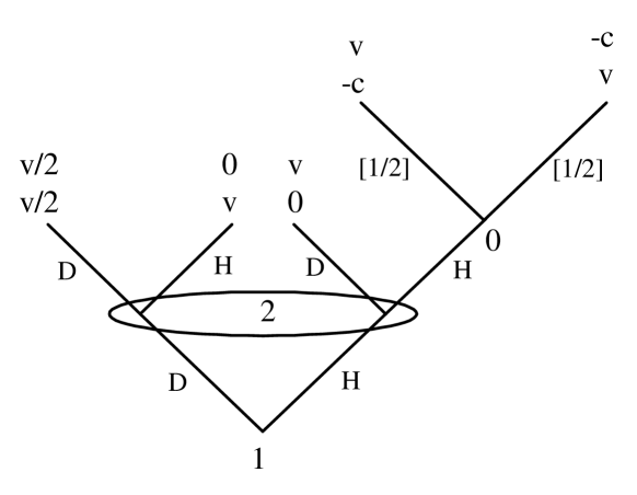
Figure 1: The extensive-form representation of the Hawk-Dove game $G(v,c)$

Individuals accumulate payoffs over time, depending on how they fare when playing the Hawk-Dove game with randomly drawn opponents. An individual’s stock of accumulated payoffs at any point in time is called the individual’s current wealth. Hence, an individual $i\in\left\{1,...,N\right\}$ who enters a pairwise interaction with wealth $w$, exits the interaction with wealth $w+v/2$ if both play D, with wealth $w+v$ if she plays H and her opponent plays D, and with unchanged wealth, $w$, if she plays D and the opponent plays H. If both play H, she will end up with either wealth $w+v$, which happens with probability one half, or with wealth $w-c$. In terms of total wealth in the population, all three strategy profiles DD, DH and HD thus result in an increase by $v$, while the strategy profile HH, to be called a fight, results in a net increase of population wealth by $v-c$. For analytical convenience, we henceforth assume that $c$ and $v$ are positive integers and that $v$ is even.

A pure or mixed strategy in a finite and symmetric two-player game is evolutionarily stable, or an ESS (Maynard Smith and Price, 1973) if it is a best reply to itself and a better reply to all other best replies. Hence, it is a refinement of symmetric Nash equilibrium, a refinement that captures resistance against any "mutant" strategy that appear in a sufficiently small population share. The Hawk-Dove game has a unique ESS, namely to use strategy H with probability

$$x^{\ast}=\min\left\{1,v/c\right\}.$$

The expected payoff when both parties use this strategy is

$$\pi^{\ast}=\max\left\{\left(1-\frac{v}{c}\right)\frac{v}{2},\frac{v-c}{2}\right\}.$$

In the present model, the described strategic interaction is not the only source of wealth. Individuals also have other sources of income. For analytical convenience, the arrival time of external income is the same as the arrival time for playing the game. Each party then receives income $y/2>c$. This income adds to the gain or loss made in the pairwise game playing. The assumption $y/2>c$ guarantees that the net gain at each random match is nonnegative, thus avoiding that an individual’s wealth can become negative. In addition to receiving game payoffs and background income, every individual’s accumulated wealth is exposed to random depreciation, whereby it stochastically decreases, and may fall down to zero (but not become negative).

Formally, we model the evolution of wealth for all $N$ individuals as a Markov process $W^{N}$ in $\mathbb{N}_{0}^{N}$ over continuous time $t\geq 0$. Its state at any time $t$ is the vector $W^{N}(t)=\left(W_{1}^{N}(t),...,W_{N}^{N}(t)\right)$ of individual wealth holdings. The wealth distribution at time $t$ is the probability distribution on $\mathbb{N}_{0}^{N}$ defined by

$$\mu^{N}(t)=\frac{1}{N}\sum_{i=1}^{N}\delta_{W_{i}^{N}(t)}^{\left(i\right)}\ ,$$ (1)

where $\delta_{W_{i}^{N}(t)}^{\left(i\right)}$ is the probability distribution on $\mathbb{N}_{0}^{N}$ that assigns unit probability to the wealth vector where all components $j\neq i$ are zero and component $i$ equals $W_{i}^{N}(t)$. The associated average wealth is

$$\bar{W}^{N}(t)=\frac{1}{N}\sum_{i=1}^{N}W_{i}^{N}(t).$$ (2)

We attach to each individual a “depreciation Poisson clock” of rate $1$, and to each ordered pair of distinct individuals a “game Poisson clock” of rate $1/\left(N-1\right)$. Being statistically independent, the superposition of these Poisson processes, across the whole population, results in a stationary population Poisson process, and the accompanying population wealth process changes state precisely at its arrival times. The intensity of the aggregate population Poisson process is $\lambda=2N$. To see this, note that both the “population depreciation Poisson clock” and the “population game Poisson clock” each have intensity $N$ (the number of ordered pairs being $N\left(N-1\right)$).

When the game Poisson clock rings for two individuals, they each receive income $y/2$ and play the game $G(v,c)$. In this baseline version of the model, we assume that all individuals always use the unique evolutionarily stable strategy $x^{\ast}=\min\left\{v/c,1\right\}$ when playing the game (see Section 5 for a generalization).

When the depreciation Poisson clock rings for an individual, a random reduction occurs of the individual’s wealth. The expected reduction factor is fixed at $\delta$, and the probability for reduction to zero wealth has a uniform positive lower bound $\varepsilon$. More precisely, let $\delta\in\left[0,1\right]$ and $\varepsilon>0$. For each $k\in\mathbb{N}$, let $Z_{k}$ be a random variable that takes values in $\left\{0,1,...,k\right\}$, with $\mathbb{E}\left(Z_{k}\right)=\delta k$ and $\mathbb{P}\left(Z_{k}=k\right)\geq\varepsilon$. If $W_{i}^{N}(t)=w>0$ then depreciation replaces the individual’s current wealth $w$ by the random wealth level $w-Z_{w}$ (with statistical independence with respect to all other random events). If $W_{i}^{N}(t)=0$, then the individual’s wealth after depreciation remains at zero. Hence, the conditionally expected individual wealth level, after depreciation, given current wealth $W_{i}^{N}(t)=w>0$, is $\left(1-\delta\right)w$, and the probability for losing all wealth has a positive lower bound, $\varepsilon$, for all $w>0$. We call $\delta$ the depreciation rate.

The described events of pairwise matching for game play and individual wealth depreciation are all statistically independent. Given the Poisson clocks, the underlying game $G\left(v,c\right)$, the associated ESS $x^{\ast}$, the depreciation rate $\delta$, and probability bound $\varepsilon$, $W^{N}=\left\langle W^{N}(t)\right\rangle_{t\in\mathbb{R}_{+}}$ constitutes a Markov process in $\mathbb{N}_{0}^{N}$.

3 Asymptotics

We here provide two asymptotic results for the wealth process. First with respect to time, for a given finite population, and then with respect to population size, at a given finite observation time.

Consider a population of arbitrary fixed size, $N>1$. At any finite time $t$, the state of the wealth process is evidently history dependent. However, asymptotically over time it is not. The effect of the initial wealth distribution washes out over time an vanishes asymptotically. This is not surprising, given the nature of the process. However, to formally prove this is non-trivial, so a proof is given in the appendix for the interested reader.

Proposition 1.

The wealth process $W^{N}$ is ergodic, and thus has a unique invariant distribution to which it converges in distribution from any initial state.

Second, we instead consider the distribution of individual wealth at any fixed and given time $t$ when the population is very large. To be more specific, we analyze the probability distribution for any given individual’s wealth at a given time $t>0$ in the limit as $N\rightarrow+\infty$. For this purpose, let $\mathcal{L}(X)$ denote the probability distribution of any random variable $X$, and let $\left(\mathcal{L}(X_{i})\right)^{\otimes k}$ be the product probability distribution of $k$ such i.i.d. random variables $X_{i}$.

Suppose that the initial individual wealth levels, the random variables $W_{i}^{N}(0)$, for $i=1,...,N$, are i.i.d. $\pi$, irrespective of population size $N$. Then one can establish the following "propagation of chaos" result for the arguably most interesting case when the Hawk-Dove game is not dominance solvable, that is, when $v<c$.

Proposition 2.

Suppose that $v<c$ and that all individuals always use strategy $x^{\ast}$. For any initial probability distribution $\pi$, the evolution of individual wealth can be represented by a Markov process $\tilde{W}=\left\langle\tilde{W}(t)\right\rangle_{t\in\mathbb{R}_{+}}$ in $\mathbb{N}_{0}$, with $\mathcal{L}(\tilde{W}(0))=\pi$, such that for any number $n\in\mathbb{N}$ of individuals:

$$\lim\limits_{N\rightarrow+\infty}\mathcal{L}(W_{1}^{N},\dots,W_{n}^{N})=\left(\mathcal{L}(\tilde{W})\right)^{\otimes n}.$$ (3)

Moreover, when $\mathbb{P}\left(Z_{k}\in\left\{0,k\right\}\right)=1$, then the following "propagation of chaos" differential equation holds, for any $w\in\mathbb{N}_{0}$ and $t\geq 0$:

$$\frac{\partial}{\partial t}\mathbb{P}\left[\tilde{W}\left(t\right)=w\right]\ = \ 2\left(1-\frac{v}{c}\right)^{2}\cdot\mathbb{P}\left[\tilde{W}\left(t\right)=w-v/2-y/2\right]$$

$$+\frac{2v}{c}\left(1-\frac{v}{c}\right)\cdot\left(\mathbb{P}\left[\tilde{W}\left(t\right)=w-v-y/2\right]+\mathbb{P}\left[\tilde{W}\left(t\right)=w-y/2\right]\right)$$

$$+\left(\frac{v}{c}\right)^{2}\cdot\left(\mathbb{P}\left[\tilde{W}\left(t\right)=w-v-y/2\right]+\mathbb{P}\left[\tilde{W}\left(t\right)=w+c-y/2\right]\right)$$

$$-2\cdot\mathbb{P}\left[\tilde{W}\left(t\right)=w\right]-D_{w}$$

where $D_{w}=\delta\cdot\mathbb{P}\left[\tilde{W}\left(t\right)=w\right]\$for all $w\neq 0$, and $D_{0}=\delta\cdot\mathbb{P}\left[\tilde{W}\left(t\right)=0\right]-\delta$.

The process $\tilde{W}$ can be thought of as the wealth dynamics of a representative individual. The first part of this theorem, the convergence result (3), establishes that the larger the population, the less correlated are the wealth levels within in any finite group of individuals (of fixed size $k$), and, in the limit as population size $N$ tends to infinity, these individual wealth levels become statistically independent. Moreover, the probability distribution of each individual’s wealth, $W_{i}^{N}\left(t\right)$, at any given time $t>0$, tends to the distribution of the random variable $\tilde{W}\$as population size $N$ tends to infinity.

The evolution of this probability distribution over time $t$ is given in equation (2), for the special case when depreciation takes the drastic form of either leaving the individual’s wealth untouched (with probability $1-\delta$) or making it vanish altogether (with probability $\delta$). Technically, the assumption is that for an individual with wealth $w$, the random wealth loss, $Z_{w}$ takes values in $\left\{0,w\right\}$, that is, either all $w$ units vanish, or the individual’s wealth remains intact. Moreover, for any level of wealth $w$, $\mathbb{P}(\tilde{W}(t)=w)$ is the population share of individuals, in an infinite population, with that wealth level. The different terms in the evolution equation represent different "inflows" and "outflows" from any given wealth level $w\in\mathbb{N}_{0}$. More precisely, there are three inflows, from wealth levels $w-v/2$,$\ w-v\$and$\ w+c$, and two outflows, one because individuals are drawn to play the game and one because of depreciation of wealth. The coefficients in equation (2) can be obtained from Figure 1 by multiplying probabilities downwards from the terminal nodes to the root of the tree, under the hypothesis that individual $i$ at the root has wealth $w$, and using the fact that the average time rate of game-playing for an individual is always 2, also in the limit as $N\rightarrow\infty$. The wealth level zero, however, is special, if $\delta>0$, in that it has no depreciation outflow. Instead, it has an extra inflow, emanating from depreciation of the wealth of individuals with non-zero wealth.

One may use equation (2) to derive the laws of motion for the first and second moments of the distribution of a representative individual’s wealth at any point in time, granted the depreciation rate is positive.

Corollary 1.

Suppose that (a) $v<c$, (b) depreciation is such that $\mathbb{P}\left(Z_{k}\in\left\{0,k\right\}\right)=1$, (c) all individuals always use strategy $x^{\ast}$, and (d) the initial individual wealth distribution $\pi$ has finite mean and variance. There then exist constants $K_{1},K_{2},K_{3},K_{4}\in\mathbb{R}$ such that

$$\mathbb{E}\left[\tilde{W}(t)\right]\ =\ \frac{1}{\delta}\left[\left(1-\frac{v}{c}\right)v+y\right]+K_{1}e^{-\delta t}\quad\forall t\geq 0$$ (5)

$$Var\left[\tilde{W}(t)\right]\ =\ \frac{1}{\delta^{2}}\left[\delta A+\left(1-\frac{v}{c}\right)^{2}v^{2}+y^{2}-2\frac{v}{c}vy\right]+K_{2}e^{-\delta t}+K_{3}e^{-2\delta t}+K_{4}te^{-\delta t}\quad\forall t\geq 0.$$ (6)

for

$$A=\frac{1}{2}\left[4-\left(1-\frac{v}{c}\right)^{2}\right]v^{2}+\frac{1}{2}\left[\left(2-\frac{v}{c}\right)\frac{v}{y}+1\right]y^{2}.$$

In other words, the first and second moments converge exponentially over time to their asymptotic values,

$$\lim_{t\rightarrow\infty}\mathbb{E}\left[\tilde{W}(t)\right]=\frac{1}{\delta}\left[\left(1-\frac{v}{c}\right)v+y\right]$$ (7)

and

$$\lim_{t\rightarrow\infty}Var\left[\tilde{W}(t)\right]=\frac{1}{\delta^{2}}\left(\delta A+\left(1-\frac{v}{c}\right)^{2}v^{2}+y^{2}-2\frac{y}{c}v^{2}\right)$$ (8)

It follows that the asymptotic coefficient of variation (also known as "relative standard deviation"), is decreasing in the depreciation rate $\delta$ and, as the this rate $\delta$ tends zero, the coefficient of variation tends to

$$\lim_{\delta\rightarrow 0}\lim_{t\rightarrow+\infty}\frac{\sqrt{Var(\tilde{W}(t))}}{\mathbb{E}(\tilde{W}(t))}=\frac{\sqrt{\left[\left(1-\frac{v}{c}\right)v+y\right]^{2}-2yv}}{\left(1-\frac{v}{c}\right)v+y}$$ (9)

The variation of an individual’s wealth has three sources. First the stochastically arriving income $y/2$. Second, the strategic interaction, which gives rise to gains and losses, a source represented by the game parameters $v$ and $c$, where $v<c$. Third, the depreciation of individual wealth, a source represented by the parameter $\delta$, here taken down to zero. We note that the limit coefficient of variation, when $\delta\downarrow 0$, is always less than one, and that it equals one in the absence of the exogenous income $y$, for any values $v<c$. We conjecture that this invariance is due to the equilibrium nature of individual behavior, the probability $x^{\ast}$. For both pure strategies, H and D, then result in the same expected net wealth gain.

The wealth distribution is different when the depreciation hits less dramatically than assumed in the above calculations. For example, suppose that depreciation can take two forms, where the first is the same as above, that is, that an individual’s all wealth vanishes with probability $\delta$, while the second form is that each unit of an individual’s wealth vanishes with the same probability $\delta$ and that this event is statistically independent among wealth units. Suppose moreover, that the first form of depreciation has probability $\rho$ and the second has probability $1-\rho$, and assume that all these random variables are statistically independent. Hence, in the second case, the number $Z_{w}$ of depreciated wealth units is binomially distributed, $Bin\left(w,\delta\right)$. See diagram below.

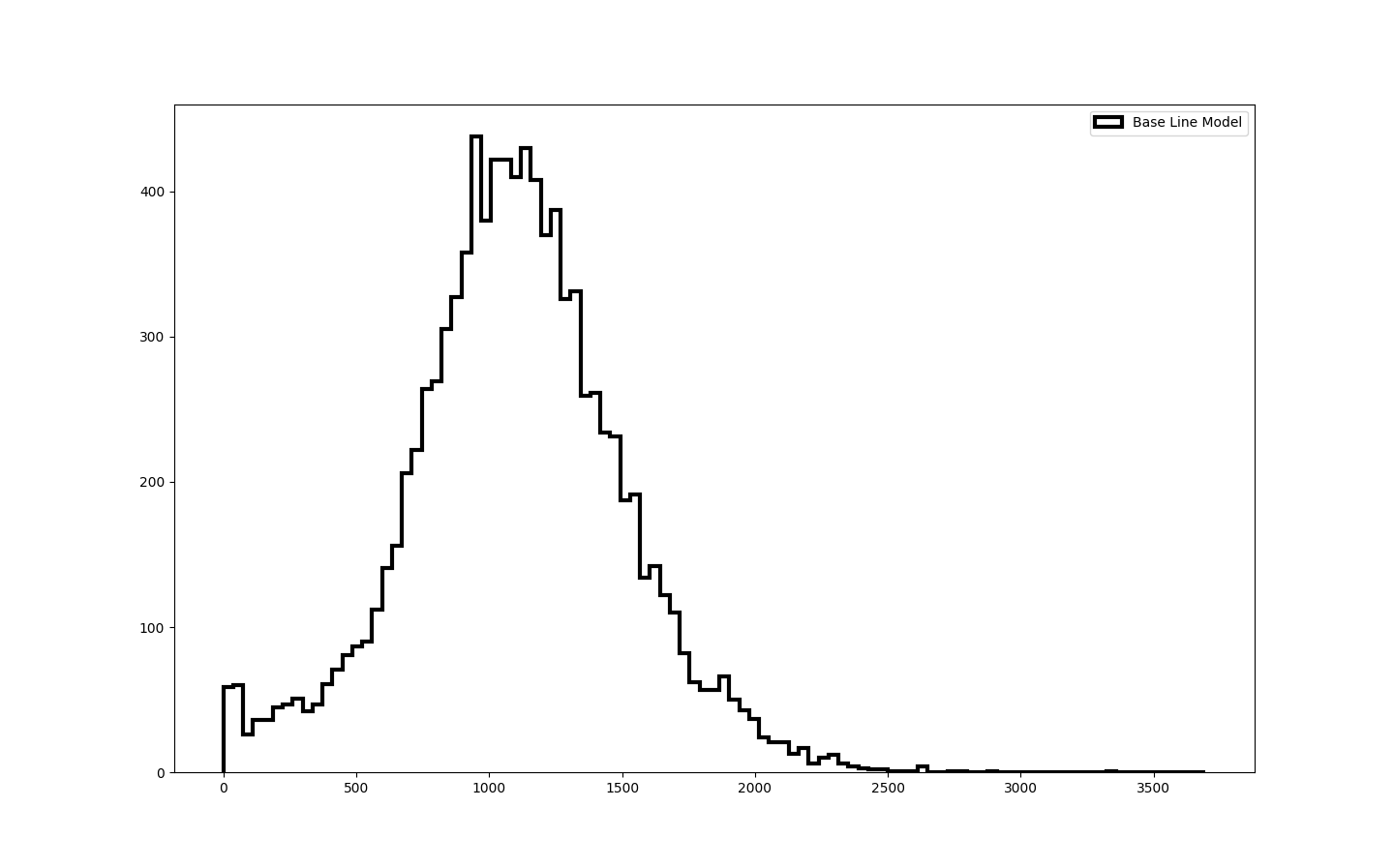
Figure 2: Empirical long-run wealth distribution under partly binomial depreciation.

The figure shows simulation results for $v=40$, $c=20$, $y=100$, $\delta=0.1$, $N=10,000$, $T=10,000,000$, and $\rho=1/10$. In this simulation, the empirical average (with respect to a given individual) is approximately 1098, the standard deviation is 403, the median 1095, the maximum wealth 3347, and the Gini coefficient 0.2. We note that the empirical coefficient of variation thus is approximately 0.37, while the theoretical asymptotic value for $\rho=1$, according to (9), is approximately 0.44. As expected, the less drastic version of depreciation induces a lower coefficient of variation.

4 Average wealth

Let $T$ be any arrival time of the above Poisson process and let $\bar{W}^{N}(T)$ be average wealth in the population at this time, defined in (2). Hence, "population wealth, or "national wealth" is $N\bar{W}^{N}(T)$. At this arrival time $T$, one of two equally probable events will take place: either one individual is selected for wealth depreciation, or an ordered pair of individuals are selected to receive income and play the game $G\left(v,c\right)$.

In the first event, the wealth of one randomly drawn individual is taken to zero with probability $\delta$. Accordingly, average wealth in the population then decreases by a random integer amount $Y^{N}$ (depending on the wealth of the randomly drawn individual), the expected value of which, conditional upon $\bar{W}^{N}(T)$, is $\delta\cdot\bar{W}^{N}(T)/N$. In the second event, there is a positive probability that the two matched individuals will fight, that is, both play H, and this probability is $\left(x^{\ast}\right)^{2}=\left(\min\left\{1,v/c\right\}\right)^{2}$. When this happens, average wealth will change by $\left(v-c\right)/N$. If they will not both fight, then no wealth is lost in their interaction, and average wealth increases by $v/N$.

In sum, average wealth at all times $t\in[T,T^{\prime})$, where $T^{\prime}$ is the next arrival time, is determined as follows:

$$\bar{W}^{N}(t)\quad=\quad\bar{W}^{N}(T)\ +\ \frac{1}{N}\cdot\left\{\begin{array}[]{ll}-Y^{N}&\text{{\small with probability}{\ }}\frac{1}{2}\\ v-c+y&\text{{\small with probability}{\ }}\frac{1}{2}\left(\min\left\{1,v/c\right\}\right)^{2}\\ v+y&\text{{\small otherwise}}\end{array}\right..$$ (10)

This defines a stochastic process $\bar{W}^{N}$ that, however, is not a Markov process. The reason is that when the population depreciation Poisson clock strikes, the statistical distribution of depreciation depends on the current wealth distribution. Average wealth falls more if a rich individual, instead of a poor individual, is hit by "drastic depreciation".

4.1 The case $v<c$

In this classical case in evolutionary game theory, the unique evolutionarily stable strategy in $G\left(v,c\right)$ is to play H with probability $x^{\ast}=v/c$. If everybody else in the population uses this strategy, then it is an optimal strategy for any individual who strives to maximize his or her expected net wealth gain in each interaction. If all individuals play $x^{\ast}=v/c$ in all matchings, then the probability for a fight (HH) in a random match is $q^{\ast}=v^{2}/c^{2}$.

One would guess that when $N$ is large, then the average-wealth process follows closely the solution trajectories of its mean-field equation. To make this precise, suppose that all individuals in all matches play the unique ESS, $x^{\ast}=v/c$. Taking expectations in (10) suggests a simple time-homogeneous ordinary differential equation for the dynamics of expected average wealth, from any initial state.

Proposition 3.

Let $w(t)=\mathbb{E}\left[\bar{W}^{N}\left(t\right)\mid\bar{W}^{N}\left(0\right)=w_{0}\right]$, and suppose that $\delta>0$. Then

$$\dot{w}(t)=v\left(1-\frac{v}{c}\right)+y-\delta w(t)\quad\forall t\geq 0,$$ (11)

with initial value $w\left(0\right)=w_{0}$.

In the Appendix we prove this by using infinitesimal generators. This simple mean-field equation has a unique solution, namely,

$$w(t)=\left(1-\frac{v}{c}\right)\frac{v}{\delta}+\frac{y}{\delta}+\left(w_{0}-\left(1-\frac{v}{c}\right)\frac{v}{\delta}-\frac{y}{\delta}\right)e^{-\delta t}\mathsf{\quad}\forall t\geq 0\text{.}$$ (12)

Irrespective of the initial wealth level $w_{0}\geq 0$, this solution converges asymptotically to the unique steady-state level (see Corollary 1)

$$w^{\ast}=\left(1-\frac{v}{c}\right)\frac{v}{\delta}+\frac{y}{\delta}=\lim_{t\rightarrow\infty}\mathbb{E}\left[\tilde{W}(t)\right].$$ (13)

We also note that average wealth increases linearly over time in the absence of depreciation: for $\delta=0$, the solution to (11) is

$$w(t)=w_{0}+yt+v\left(1-\frac{v}{c}\right)t\ \quad\forall t\geq 0,$$ (14)

for any initial wealth level $w_{0}{\geq 0}$.

4.2 The case $v>c$

What happens if the opportunity value $v$ exceeds the damage cost $c$? As noted above, it is then always optimal to play strategy H. Suppose that this is what all individuals do. Then the the mean-field equation for average wealth becomes

$$\dot{w}(t)=y+v-c-\delta w(t).$$ (15)

Accordingly, all solutions, irrespective of initial conditions, converge to the steady state level

$$w^{\ast}=\frac{y+v-c}{\delta}.$$ (16)

The above approximation result, Proposition 3, holds as stated with equation (11) replaced by equation (15). Also in this case average wealth would increase linearly over time in the absence of depreciation:

$$w(t)=w_{0}+\left(y+v-c\right)t\ \quad\forall t\geq 0.$$ (17)

4.3 Comparative statics

Combining equations (13) and (16) we obtain the following general expression for the unique steady-state level of average wealth, associated with any positive depreciation rate $\delta$:

$$w^{\ast}=\max\left\{\frac{y+v-v^{2}/c}{\delta},\frac{y+v-c}{\delta}\right\}.$$ (18)

Not surprisingly, average wealth is lower the higher is the depreciation rate. However, the equation also shows a feature that may be less expected, namely, that steady-state average wealth is non-monotonic in both the value $v$ of the stake in the pairwise opportunities and in the cost $c$ of a lost conflict. This is illustrated in the two diagrams below. Figure 3 shows steady-state average wealth as a function of $v$, for $c=40$, $y=100$ and $\delta=0.1$. The dashed horizontal line indicates steady-state wealth in the absence of the pairwise interaction. Figure 4 again shows steady-state wealth, but now as a function of $c$, for $v=20$, $y=100$ and $\delta=0.1$.

Figure 3: Steady-state average wealth as a function of the value $v$ in game $G(v,c)$.

Figure 4: Steady-state average wealth as a function of the cost $c$ in game $G(v,c)$.

The reason why the game adds nothing to the steady-state wealth level $w^{\ast}$ when $v=c$ is that then all matched pairs have a fight, whereby one party wins $v$ and the other loses just as much. Consequently, for such game parameters, average wealth converges over time to the steady-state level $y/\delta=1000$, from any initial level. The reason why steady-state wealth is also non-monotonic in the cost $c$ of losing a conflict, is the other side of the same coin. For $c<v$, H dominates D, and thus all pairs fight, and each time the net gain is $v-c$, a gain that decreases linearly in $c$. When $c$ has risen to $v$, the net gain is zero, and for higher $c$, the probability for a fight is $v^{2}/c^{2}$, a decreasing function of $c$, so the expected net gain in a random match is $v-v^{2}/c$, an increasing function of $c$. The more damage an individual who loses a conflict suffers, the fewer conflicts there are in equilibrium, and the wealthier will society be in steady state. Hence, contrary to what one might first think, a reduction of the damage due to a fight may increase the frequency of fights enough to reduce steady-state wealth.

5 When wealth is strength

So far, we have assumed that all individuals have the same chance of winning a fight. Arguably, wealthier individuals usually have a higher probability of winning conflicts. In the animal kingdom, "wealth" may be body weight, muscular mass, or control of a good territory, while among humans, wealth may consist in part in buildings and weaponry, or availability of good lawyers. We here briefly outline how our base-line model can be generalized to allow for "wealth is strength".

Consider the slight generalization of the (symmetric) HD game $G\left(v,c\right)$ to the (potentially asymmetric) HD game $G^{\ast}\left(v,c,p\right)$ shown in the diagram below, where $p\in\left[0,1\right]$ is the (exogenous) probability that player 1 will win a fight. We note that the original Hawk-Dove game is the special case when $p=1/2$.

Figure 5: The slightly generalized Hawk-Dove game $G^{*}(v,c,p)$.

For brevity, we henceforth focus on the case when $v<c$.

Consider two individuals in the population, $i$ and $j$, who just have been matched to play the extended HD game $G\left(v,c,p\right)$, where player 1’s success probability $p$ depends on their wealth levels. More precisely, if individual $i$ has wealth $w_{i}$ and is in player role 1, and individual $j$ has wealth $w_{j}$ and is in player role 2, then $p=f(w_{i},w_{j})$, where $f:\mathbb{R}^{2}\rightarrow\left[0,1\right]$ is the logistic version of Tullock’s contest function (Tullock (1980)):

$$f(w_{i},w_{j})=\frac{e^{\sigma w_{i}}}{e^{\sigma w_{i}}+e^{\sigma w_{j}}}.$$ (19)

Here $\sigma\geq 0$ is a parameter that represents the sensitivity of the success probability $p$ to the wealth difference between the fighters. It is increasing in own wealth, $w_{i}$, decreasing in the opponent’s wealth, $w_{j}$ and equals one half for any value of $\sigma$, when $w_{i}=w_{j}$. The success probability is also one half when $\sigma=0$, irrespective of the wealth levels (just as in game $G\left(v,c\right)$). We also note that it is immaterial which player role, 1 or 2, that individuals are assigned to (if $i$ is assigned player role 2, then $p=f(w_{j},w_{i})=1-f\left(w_{i},w_{j}\right)$).

A number of relevant information scenarios open up. In one scenario, each individual only knows his or her own wealth. In another scenario, any two matched individuals observe each others’ wealth. In a third scenario, each individual in a match knows her own wealth and receives a noisy private signal about the opponent’s wealth. We here focus on the second scenario, for $\sigma>0$.

It is easily verified that strategy $H$ strictly dominates strategy $D$ for individual $i$ (irrespective of player role) if and only if his or her winning probability is sufficiently high, $f(w_{i},w_{j})>c/\left(v+c\right)$, a condition that is equivalent with

$$w_{i}-w_{j}>\frac{1}{\sigma}\ln\left(\frac{c}{v}\right).$$ (20)

The set of Nash equilibria of $G\left(v,c,p\right)$, when played between individual $i$ in player role 1 and individual $j$ in player role 2, depends on the parameters as follows (see Appendix for a proof):

Proposition 4.

Suppose that $v<c$. If (20) holds, then the unique Nash equilibrium is $(H,D)$. If

$$\left|w_{i}-w_{j}\right|<\frac{1}{\sigma}\ln\left(\frac{c}{v}\right),$$ (21)

then there are three Nash equilibria: $(H,D)$, $(D,H)$, and a mixed equilibrium in which individual $i$ plays $H$ with probability

$$x^{\ast}=\frac{v}{2\left(v+c\right)f(w_{i},w_{j})-v}$$ (22)

and individual $j$ plays $H$ with probability

$$y^{\ast}=\frac{v}{2\left(v+c\right)f(w_{j},w_{i})-v}.$$ (23)

In sum: when wealth levels are sufficiently apart, the poorer individual plays D and the richer plays H. The rich individual then takes the whole "cake" without fight. When wealth levels are not far apart, but not identical, there are three candidate equilibria. In one equilibrium, the rich individual takes the cake without fight, in another, the poor individual takes the cake without fight, and in the third equilibrium they both randomize between H and D, but with slightly different probabilities. Irrespective of which equilibrium is played in such encounters, the general level of fighting in the population is lower than in the base-line Hawk-Dove model. This conclusion is in line with McNamara and Houston, 2005. (However, a difference between our model and theirs is that in their model, the two contestants don’t know the other contestant’s fighting ability). If the wealth levels happen to be identical, then we are back to the base-line model.

Remark 1.

It is well-known in biology that animals who contest a resource many times avoid fighting, and thereby avoid damage, by way of judging each other’s strength. Contestants also often try to impress each other by demonstrating or exaggerating their fighting ability. Usually, fights occur only if the two contestants appear approximately equally strong. Arguably, avoidance of conflicts between unequal individuals are also common among humans. For mathematical models of animal fighting, see Enquist and Leimar (1983, 1984, 1987, 1990), Houston and McNamara (1988), Crowley (2000), and McNamara and Houston (2005). In Houston and McNamara (1988), individuals have different ‘energy reserve’ levels, and the ESS has the form ‘play H if your energy reserves are below a certain critical value, otherwise play D’. Crowley (2000) analyze both the case when individuals only know their own fighting ability and when they also know their opponent’s ability. In McNamara and Houston (2005), where each individual knows only his or her own fighting ability, the ESS takes the form of a threshold for switching from D to H as own fighting ability rises. None of the mentioned studies analyzes the associated stochastic accumulation processes.

A possible scenario is that the mixed equilibrium is played whenever (21) holds; and this is in line with the empirical observation that fighting seems to take place mostly between parties that are relatively equal in strength. Formally, the equilibrium strategy for an individual in the population game (where all individuals are players who are randomly called upon for pairwise play) can then be defined as a function $\xi$ of own wealth, $w$, and the opponent’s wealth, $w^{\prime}$:

$$\xi\left(w,w^{\prime}\right)=\mathbb{P}\left(H\mid w,w^{\prime}\right)=\left\{\begin{array}[]{ll}\quad 1&\text{if }w-w^{\prime}>\sigma^{-1}\ln\left(c/v\right)\\ \frac{v}{2\left(v+c\right)f(w,w^{\prime})-v}&\text{if }\left|w-w^{\prime}\right|\leq\sigma^{-1}\ln\left(c/v\right)\\ \quad 0&\text{if }w^{\prime}-w>\sigma^{-1}\ln\left(c/v\right)\end{array}\right.$$

However, as shown in Selten (1980), mixed equilibria are not played in evolutionarily stable role-conditioned strategies. Hence, evolutionary stability requires that either $(H,D)$ or $(D,H)$ is played when $0<\left|w-w^{\prime}\right|\leq\sigma^{-1}\ln\left(c/v\right)$. The following population-game strategy is evolutionarily stable:

$$\xi^{\ast}\left(w,w^{\prime}\right)=\mathbb{P}\left(H\mid w,w^{\prime}\right)=\left\{\begin{array}[]{ll}\quad 1&\text{if }w>w^{\prime}\\ v/c&\text{if }w=w^{\prime}\\ \quad 0&\text{if }w^{\prime}<w\end{array}\right.$$

Figure 6 below compares the long-run wealth distribution for $\sigma=1$, under population strategy $\xi^{\ast}$, with the base line-case when $\sigma=0$, for the same parameter values as in Figure 2 (but with slightly different resolution). Not surprisingly, the distribution is more dispersed and average wealth is somewhat higher (because of the avoidance of fights). The empirical average in this simulation is $1206$, standard deviation $506$, median $1177$, maximum $3625$, and the Gini coefficient is $0.23$. Compared with the base line model, with equal probability of winning a fight, the empirical average, median, maximum increased almost $10$%, the Gini coefficient by $15$%, and the standard deviation by about $25$%.

Figure 6: The long-run distribution of individual wealth when "wealth is strength", compared with the distribution in the base-line model.

When individuals’ strategies are state-dependent, as in the present model of "wealth is strength", some previous results for the base line model still hold. In particular, the proof of Proposition 1 doesn’t change when wealth is strength. Hence, the wealth process is still ergodic. The fact that individuals know their own wealth and the wealth of their opponent brings non-linearity into the proof of the propagation of chaos. For a proof of propagation-of-chaos for a similar but non-linear wealth accumulation process, see Gibaud (2016). Based upon that proof, we claim that the propagation of chaos holds also when wealth is strength. However, since the evolution equations change, so will Corollary 1.

6 Discussion

The purpose of this study was to work out an analytical framework that permits rigorous mathematical analysis of mechanisms at work in the accumulation and distribution of wealth, a framework that would allow extensions and generalizations to richer and more realistic models.

For instance, instead of having only one game played—here a simple Hawk-Dove game—there could be a family of more or less complex $n$-player games (for $n=1,2,3...$) representing opportunities for production, trade, bargaining etc., games that are randomly drawn according to some (exogenous or endogenous) probability distribution. Individuals may then be given the option of not taking part in an interaction, which can easily be obtained by adding a pure strategy, that if chosen by a participant, leaves that individual’s wealth untouched (and that affects other participants’ material payoffs in a prescribed way). We hope that the present analytical framework, in suitably extended forms, may help understand mechanisms behind the accumulation and distribution of wealth, see e.g. Bardhan, Bowles and Gintis (1999), Davies and Shorrock (1999), and Picketty (2014).

The present analysis rests upon other heroic and unrealistic assumptions. An important ingredient that is missing in the present model framework is consumption. What we here call “depreciation” can of course be thought of as “consumption”. Evidently, this is a rather mechanical way of treating such an activity. An interesting extension would therefore be to include endogenous consumption decisions made by (potentially risk averse) individuals with (some) foresight. And perhaps just as importantly, individual motivation may be much more complex, involving altruism or spite, inequity aversion and/or morality etc.

To mention but one more potential extension: endogeneity of the process that creates the opportunities. Arguably, both the values of opportunities and their arrival rates depend in a positive way on current and past national wealth. Such endogenous growth by way of positive feed-backs may turn the present ergodic wealth processes into so-called explosive processes for which it may be possible to identify stable growth paths. While such generalizations may raise substantial mathematical challenges, they would be highly relevant for understanding real-world phenomena and amenable to numerical computer simulations.

Another avenue for future research is laboratory experiments, much in line with computer games. One could imagine experiments based on models such as the ones analyzed here but also more complex versions, with a large number of human subjects who each is given the role of a specific individual $i$ in the population. Just as in our theoretical framework, individuals would be exogenously and randomly matched for anonymous strategic interaction — they would then not be informed of the identity of the other participants in the interaction at hand, only of the game strategies and payoffs in question and their own role assignment in that game (which may be symmetric or asymmetric). At the end of a long such experimental session, each subject could be paid according to his or her final wealth. The results from such experiments could then be compared with theoretical predictions and numerical simulations along the lines given here.

The topics of wealth accumulation and wealth distribution are of course big in the economics literature. Despite this, the models used in that literature seem to differ starkly from ours. To the best of our knowledge, neither the present model framework nor our analytical results are closely related to other work in the economics literature. Indeed, we would be grateful for suggestions for references to potentially related work. The closest branch of economics seems to be the search literature, with perhaps Rubinstein and Wolinsky (1990) coming nearest us. We hope that generalizations of the present model framework will enable novel analyses of the accumulation and distribution of fitness and wealth.

7 Appendix

The proofs in this appendix are adaptations to the present setting of proofs for more general results in Gibaud (2016).

7.1 Notation and preliminaries

Let $N\in\mathbb{N}$, for $N>1$, be population size, and let $F$ denote the state-space, where either $F=\mathbb{N}_{0}^{N}$ or $F=\mathbb{R}$. Denote by ${C}_{c}^{\infty}(F)$ the set of real-valued smooth (infinitely differentiable) functions defined on $F$. Let $C_{b}(F)$ be the space of continuous and bounded functions from $F$ to $\mathbb{R}$. As usual, $\|.\|_{\infty}$ represents the sup norm on bounded functions, and $|||.|||$ denotes the operator norm on ${C}_{b}(F)$, that is, $|||L|||\ =\sup_{f\in C_{b}(F)}\frac{\|Lf\|_{\infty}}{\|f\|_{\infty}}$.

A (continuous time) stochastic process $X=\left\langle X(t)\right\rangle_{t\geq 0}$ in $F$ is a random variable taking values in $D(\mathbb{R}_{+},F)$, the space of right-continuous left-limited functions, from $[0,+\infty)$ to $F$. We will consider Markov processes with initial distribution $\nu$, a probability measure on $F$, and transition matrix, to be called the rate matrix, $(\mathcal{A}(x,y))_{x,y\in F}$, with $\mathcal{A}(x,x)=-\sum\nolimits_{y\in F\backslash\left\{\ x\right\}}\mathcal{A}(x,y)$. For $x\neq y$, $\mathcal{A}(x,y)$ is the transition rate from state $x$ to state $y$. The generator associated with this matrix is the bounded linear operator $\mathcal{A}$ that sends all bounded and Borel measurable functions $f$ from $F$ to $\mathbb{R}$, such that for all $x\in F$:

$$\mathcal{A}f(x)=\sum\limits_{y\in F}\mathcal{A}(x,y)[f(y)-f(x)].$$

Conversely, from a given generator one can construct the associated rate matrix from the factors by which the differences $[f(y)-f(x)]$ are multiplied in the expression of the generator.

Let thus $\mathcal{A}$ be any rate matrix and $\nu$ any probability measure on $F$. We will construct a Markov process $X$ as follows. First, let $\left\langle Y(n)\right\rangle_{n\in\mathbb{N}}$ be a Markov chain (over discrete time $n$) in $F$, with no absorbing states, and with initial distribution $\nu$ and transition matrix $\left(\frac{\mathcal{A}(x,y)}{|\mathcal{A}(x,x)|}\right)$. Then $\mathcal{A}(x,x)\neq 0$ since there are no absorbing states. Let $\Delta_{0}$, $\Delta_{1}$,$\dots$, be independent and exponentially distributed random variables with mean value 1. These are the time intervals between arrivals, and assume that they are statistically independent of the chain $Y$. We define the Markov process $\left\langle X(t)\right\rangle_{t\geq 0}$ in $F$, with initial distribution $\nu$ and generator $\mathcal{A}$, by:

$$X(t)=\left\{\begin{array}[]{ll}Y(0)&\text{for }0\leq t<\frac{\Delta_{0}}{|\mathcal{A}(Y(0),Y(0))|}\\ Y(k)&\text{for }\sum\limits_{j=0}^{k-1}\frac{\Delta_{j}}{|\mathcal{A}(Y(j),Y(j))|}\leq t<\sum\limits_{j=0}^{k}\frac{\Delta_{j}}{|\mathcal{A}(Y(j),Y(j))|}\end{array}\right.$$

In the present application, we divide the construction of the Markov process $W^{N}=(W_{1}^{N},\dots,W_{N}^{N})$ in two parts, where Part 1 is the random matching of pairs of individuals to play the game, and Part 2 the depreciation of individuals’ wealth.

[Part 1] At the arrivals of a Poisson process with intensity $\lambda=N$ a pair of individuals are drawn from the population to play the game. At each pairwise match, the two individuals make their choices simultaneously and independently. If all individuals use the unique ESS strategy $x^{\ast}$, then they play (D,D) with probability $p_{DD}=\left(1-v/c\right)^{2}$, (D,H) or (H,D) with probability $p_{DH}=\left(1-v/c\right)v/c$, and (H,H) with probability $p_{HH}=\left(v/c\right)^{2}$. The generator associated to this part of the wealth process is $\mathcal{A}_{g}^{N}$, with domain ${C}_{b}(\mathbb{N}_{0}^{N})$ and defined for all $f\in{C}_{b}(\mathbb{N}_{0}^{N})$ and $w\in\mathbb{N}_{0}^{N}$ by

$$\mathcal{A}_{g}^{N}\left[f(w)\right]=N\cdot\sum\limits_{\begin{subarray}{c}(i,j)\in\{1,\dots N\}^{2}\\ i\neq j\end{subarray}}\left(\begin{array}[]{l}\frac{p_{DD}}{N(N-1)}\cdot\left[f\left(w+\left(v+\frac{y}{2}\right)(e_{i}+e_{j})\right)-f(w)\right]\\ +\frac{p_{DH}}{N(N-1)}\cdot\left[f\left(w+\left(v+\frac{y}{2}\right)e_{i}+\frac{y}{2}e_{j}\right)-f(w)\right]\\ +\frac{p_{DH}}{N(N-1)}\cdot\left[f\left(w+\left(v+\frac{y}{2}\right)e_{j}+\frac{y}{2}e_{i}\right)-f(w)\right]\\ +\frac{p_{HH}}{N(N-1)}\cdot\left[\begin{array}[]{l}\frac{1}{2}\left(f\left(w+\left(v+\frac{y}{2}\right)e_{i}+\left(-c+\frac{y}{2}\right)e_{j}\right)-f(w)\right)\\ +\frac{1}{2}\left(f\left(w+\left(v+\frac{y}{2}\right)e_{j}+\left(-c+\frac{y}{2}\right)e_{i}\right)-f(w)\right)\end{array}\right]\end{array}\right),$$ (24)

where $\left\{e_{1},\dots e_{N}\right\}$ is the canonical basis of $\mathbb{R}^{N}$. The game interaction between any given two individuals $i\neq j$ occurs at the arrivals of a Poisson Process with intensity $1/\left(N-1\right)$, a process we denote $\mathcal{N}^{i,j}$.

[Part 2] In the population at large, individual wealth depreciation occurs at the arrivals of an independent Poisson process, also with intensity $\lambda=N$. At each arrival time, one individual $i$ is randomly drawn for wealth depreciation and looses all or part of his or her current wealth, $w_{i}$, according to the distribution of the random variable $Z_{w_{i}}$. The depreciation action has a generator $A_{d}^{N}$ with domain ${C}_{b}(\mathbb{N}_{0}^{N})$, defined for all $f\in{C}_{b}(\mathbb{N}_{0}^{N})$ and $w=(w_{1},\dots,w_{N})\in\mathbb{N}_{0}^{N}$. Write $z_{i}(k)$ for $\mathbb{P}(Z_{w_{i}}=k)$, for $k=0,1,...,w_{i}$. We have for all $w=(w_{0},\dots,w_{N})\in\mathbb{N}_{0}^{N}$ and $i=1,...N$ that $\sum_{k=0}^{w_{i}}kz_{i}(k)=-\delta w_{i}$ and $z_{i}(w_{i})\geq\varepsilon>0$. The depreciation infinitesimal generator is

$$\mathcal{A}_{d}^{N}[f(w)]=\sum_{i=1}^{N}\sum_{k=0}^{w_{i}}z_{i}(k)[f(w-ke_{i})-f(w)]$$ (25)

For any given individual $i\in\{1,\dots,N\}$, the depreciation Poisson process $\bar{\mathcal{N}}^{i}$ has intensity $1$, and at each arrival of this process, individual $i$ looses wealth according to the distribution of $Z_{i}$. On average, the individual looses $\delta$ times her current wealth. For any individuals $i$, $k$ and $h$, where $k\neq h$, the processes $\bar{\mathcal{N}}^{i}$ and $\mathcal{N}^{k,h}$ are independent.

Hence, the infinitesimal generator of $\left(W^{N}(t)\right)_{t\geq 0}$ is:

$$\mathcal{A}^{N}\left[f(w)\right]=\mathcal{A}_{g}^{N}\left[f(w)\right]+\mathcal{A}_{d}^{N}f(w)$$ (26)

The following notation will be convenient in the sequel: for all $w\in\mathbb{N}_{0}$, write $\Delta f(w)$ for

$$\Delta f(w)= \ 2p_{DD}\left[f\left(w+\frac{v}{2}+\frac{y}{2}\right)-f(w)\right]$$

$$+p_{DH}\left[f\left(w+v+\frac{y}{2}\right)-f(w)\right]$$

$$+p_{DH}\left[f\left(w+\frac{y}{2}\right)-f(w)\right]$$

$$+p_{HH}\left(\left[f\left(w+v+\frac{y}{2}\right)-f(w)\right]+\left[f\left(w-c+\frac{y}{2}\right)-f(w)\right]\right)$$

Let $f\in C_{b}(\mathbb{N}_{0})$. Then $f^{\prime}=(f,0,\dots,0)\in C_{b}(\mathbb{N}_{0}^{N})$, and write

$$L\left(f(w)\right)=\Delta f(w)+\sum_{k=0}^{w}z_{i}(k)\left[f(w-k)-f(w)\right].$$ (27)

Then $L(f(w))=\mathcal{A}f^{\prime}(w)$, the infinitesimal generator of the Markov process $\left(W_{i}^{N}(t)\right)_{t}$ for each $i\in\{1,\dots,N\}$.

7.2 Proof of Proposition 1

Let $N$ be a positive integer, population size, and let $\left\langle W_{n}^{N}\right\rangle_{n\in\mathbb{N}_{0}}$ be the Markov chain associated with the Markov process $\left\langle W^{N}\left(t\right)\right\rangle_{t\in\mathbb{R}_{+}}$. Write $\theta$ for the zero vector $\left(0,\dots,0\right)\in\mathbb{N}^{N}$. It is sufficient to show that $\left\langle W_{n}^{N}\right\rangle_{n\in\mathbb{N}_{0}}$ is irreducible, aperiodic and positively recurrent.

That it is irreducible follows from two observations, where the first is that the probability is positive that all wealth disappears from the population in period $n=N$, irrespective of the initial state: $\mathbb{P}_{w}\left[W^{N}(N)=\theta\right]>0$ for all $w\in\mathbb{N}^{N}$. The second observation is that $\left\langle W_{n}^{N}\right\rangle_{n\in\mathbb{N}_{0}}$ has exactly one equivalence class, namely, the set

$$E=\left\{w\in\mathbb{N}^{N}:\exists n\in\mathbb{N}\ \text{s.t.}\ \mathbb{P}_{\theta}\left[W_{n}^{N}=w\right]>0\right\}.$$

This establishes irreducibility. Moreover, since $\mathbb{P}_{\theta}\left(W_{1}^{N}=\theta\right)\geq\varepsilon>0$, the chain is also aperiodic.

To complete the proof of ergodicity, it thus remains to show that $\left\langle W_{n}^{N}\right\rangle_{n}$ is positively recurrent. For this purpose, one can use Lemma 6.3.20 in Bremaud (2020), which states that if $\left(X_{n}\right)_{n}$ is an irreducible Markov chain, $F$ a finite subset of its state space $E$, and $\tau(F)$ is the return time to $F$, then then the chain is positive recurrent if $\mathbb{E}_{j}\left[\tau(F)\right])<\infty$ for all states $j\notin F$. We use this lemma for $E=\mathbb{N}_{0}^{N}$ and $F=\{(0,\dots,0)\}$. The probability that the wealth of $i$ is depreciated is $\frac{\varepsilon}{2N}$ at each arrival of the Poisson process. Let $D_{i}$ be the event that the wealth of individual $i$ depreciates. Then, for all $\sigma\in\mathbb{N}_{0}^{N}$:

$$\mathbb{P}_{\sigma}(\tau\leq N)\geq\mathbb{P}_{\sigma}(\tau=N)\geq\mathbb{P}_{\sigma}(D_{1},D_{2},\dots,D_{N})\geq\left(\frac{\varepsilon}{2N}\right)^{N}.$$

Thus

$$\mathbb{P}_{\sigma}(\tau>N)\leq 1-\left(\frac{\varepsilon}{2N}\right)^{N}.$$

It follow that for all $\sigma\in\mathbb{N}_{0}^{N}$:

$$\mathbb{E}_{\sigma}(\tau) =\sum_{k\in\mathbb{N}}\sum_{l=1}^{N}(Nk+\ell)\mathbb{P}_{\sigma}(\tau=kN+\ell)$$

$$\leq\sum_{k\in\mathbb{N}}\sum_{l=1}^{N}(Nk+N)\mathbb{P}_{\sigma}(\tau>kN)$$

$$\leq\sum_{k\in\mathbb{N}}N^{2}(k+1)\mathbb{P}_{\sigma}(\tau>kN)$$

But we also have that, for all $\sigma\in\mathbb{N}_{0}^{N}$,

$$\mathbb{P}_{\sigma}(\tau>kN) =\mathbb{P}_{\sigma}(\tau>N)\mathbb{P}_{\sigma}(\tau>kN|\tau>N)$$

$$\leq\left(1-\left(\frac{\varepsilon}{2N}\right)^{N}\right)\sum_{\sigma_{1}\in\mathbb{N}_{0}^{N}}\mathbb{P}_{\sigma}(\tau>kN,W_{N}^{N}=\sigma_{1}|\tau>N)$$

$$\leq\left(1-\left(\frac{\varepsilon}{2N}\right)^{N}\right)\sum_{\sigma_{1}\in\mathbb{N}_{0}^{N}}\mathbb{P}_{\sigma}(\tau>kN|W_{N}^{N}=\sigma_{1},\tau>N)\mathbb{P}_{\sigma}(W_{N}^{N}=\sigma_{1}|\tau>N)$$

By the strong Markov property we obtain:

$$\mathbb{P}_{\sigma}(\tau>kN) \leq\left(1-\left(\frac{\varepsilon}{2N}\right)^{N}\right)\sum_{\sigma_{1}\in\mathbb{N}_{0}^{N}}\mathbb{P}_{\sigma_{1}}(\tau>(k-1)N)\mathbb{P}_{\sigma}(W_{N}=\sigma_{1}|\tau>N)$$

$$\left(1-\left(\frac{\varepsilon}{2N}\right)^{N}\right)^{k}\prod_{\ell=1}^{k}\underbrace{\sum_{\sigma_{\ell}\in\mathbb{N}_{0}^{N}}\mathbb{P}_{\sigma_{\ell-1}}\left(W_{N}^{N}=\sigma_{\ell}|\tau>(\ell-1)N\right)}_{=1}$$

$$\leq\left(1-\left(\frac{\varepsilon}{2N}\right)^{N}\right)^{k}$$

Hence, for all $\sigma\in\mathbb{N}_{0}^{N}$,

$$\mathbb{E}_{\sigma}(\tau)\leq\sum_{k\in\mathbb{N}}N^{2}(k+1)\left(1-\left(\frac{\varepsilon}{2N}\right)^{N}\right)^{k}\leq\frac{N^{2}}{\left(\frac{\varepsilon}{2N}\right)^{2N}}<+\infty,$$

which establishes that $\left\langle W_{n}^{N}\right\rangle_{n}$ is positively recurrent.

Thus $\left\langle W_{n}^{N}\right\rangle_{n}$ has a unique invariant distribution, and it converges to this from all initial distributions (see e.g. Thm VIII.6.8 in Barbe and Ledoux, 2007).

7.3 Proof of Proposition 2

Let $\left\langle u_{N}\right\rangle_{N\in\mathbb{N}}$ be a sequence of symmetric probability measures $u_{N}$ on $\mathbb{N}_{0}^{N}$. Following Sznitman (1991), we say that $\left\langle u_{N}\right\rangle_{N\in\mathbb{N}}$ is $u$-chaotic, with $u$ a probability measure on $\mathbb{N}_{0}$, if, for any finite collection $\left\{\phi_{1},\dots,\phi_{k}\right\}$ of continuous and bounded functions on $\mathbb{N}_{0}$,

$$\lim\limits_{N\rightarrow+\infty}\int\limits_{\mathbb{N}_{0}^{N}}\phi_{1}(x_{1})\dots\phi_{k}(x_{k})u_{N}\left(dx_{1}\dots dx_{N}\right)=\prod\limits_{i=1}^{k}\int\limits_{\mathbb{N}_{0}}\phi_{i}(x)u\left(dx\right).$$

The meaning of this definition, if we apply it to a fixed and finite number of individuals, when the total number $N$ of individuals in the population goes to infinity, these individuals’ wealth levels become i.i.d. with distribution $u$. The infinitesimal generator of $(W_{1}^{N},\dots,W_{N}^{N})$ is $\mathcal{A}_{g}^{N}$ defined in (26). This generator has the shape of a particle system with particles (or individuals) playing $2\times 2$-games.

Associated with $\mathcal{N}^{i,j}(t)$ and $\bar{\mathcal{N}}^{i}(t)$, let the processes $\mathcal{M}^{i,j}$ and $\bar{\mathcal{M}}^{i}$ be defined by

$$\left(\mathcal{M}^{i,j}(t)\right)_{t}=\left(\mathcal{N}^{i,j}(t)-\frac{t}{N-1}\right)_{t}\quad\text{and\quad}\left(\bar{\mathcal{M}}^{i}(t)\right)_{t}=\left(\bar{\mathcal{N}}^{i}(t)-t\right)_{t}$$

for all $t\geq 0$.

The object of interest for the proof is

$$M_{i}^{f,N}(t)\ = \ \sum_{j=1,j\neq i}^{N}\int_{0}^{t}\Delta f\left(W_{i}^{N}(s)\right)\text{d}\mathcal{M}^{i,j}(s)$$

$$\ +\int_{0}^{t}\sum_{k=0}^{W_{i}^{N}(s)}z_{i}(k)\left[f\left(W_{i}^{N}(s)-k\right)-f\left(W_{i}^{N}(s)\right)\right]\text{d}\bar{\mathcal{M}}^{i}(s)$$

Lemma 1.

For any population size $N>1$, and any pair of individuals $i\neq j$, with $i,j\in\left\{1,...,N\right\}$:

$$\mathbb{E}\left[M_{i}^{f,N}(t)M_{j}^{f,N}(t)\right]\leq\frac{4t\|f\|_{\infty}}{N-1}\ \quad\forall t>0$$ (28)

Proof: By independence:

$$\forall i \neq j:\ \left\langle\bar{\mathcal{M}}^{i},\bar{\mathcal{M}}^{j}\right\rangle=0$$

$$\forall i \neq j,\forall k:\ \left\langle\mathcal{M}^{i,j},\bar{\mathcal{M}}^{k}\right\rangle=0$$

$$\forall i \neq j,\forall k\neq h:\ \left\langle\mathcal{M}^{i,j},\mathcal{M}^{k,h}\right\rangle=0$$

By the Product Rule (Kurtz, 2001) and writing $u^{-}$ for the left limit:

$$\mathbb{E}\left[M_{i}^{f,N}(t)M_{j}^{f,N}(t)\right]=$$

$$= \mathbb{E}\left[M_{i}^{f,N}(0)M_{j}^{f,N}(0)\right]+\mathbb{E}\left(\int_{0}^{t}M_{i}^{f,N}(u^{-})\text{d}M_{j}^{f,N}(u)\right)+0+\mathbb{E}\left(\left\langle M_{i}^{f,N},M_{j}^{f,N}\right\rangle_{t}\right)$$

$$= \mathbb{E}\left(\int_{0}^{t}\Delta f\left[W_{i}^{N}(u)\right]\Delta f\left[W_{j}^{N}(u)\right]\right)\text{d}\left\langle\mathcal{M}^{i,j},\mathcal{M}^{i,j}\right\rangle_{u}$$

The claimed inequality (28) follows from the fact that $\left\langle\mathcal{M}^{i,j}\right\rangle=\mathcal{N}^{i,j}$. Q.E.D.

The next step is to establish tightness:

Lemma 2.

$\left(\mathcal{L}(W_{1}^{N})\right)_{N}$ is tight.

Proof: We apply Theorems 3.9.1 and 3.9.4 in Ethier and Kurtz (2009), and thus have to verify their hypotheses. First, let $\left(\mathcal{F}_{t}\right)_{t}$ be a filtration such that $\left\langle W^{N}(t)\right\rangle_{t}$ is $\mathcal{F}_{t}$-adapted. Since $W_{1}^{N}$ is a Markov process,

$$f(W_{1}^{N}(t))-f(W_{1}^{N}(0))-\int_{0}^{t}Lf(W_{1}^{N}(u-))du$$

is a $\left(\mathcal{F}_{t}\right)_{t}$-martingale. (And this of course applies to any individual $i$.)

Since the jumping rates and amplitudes are uniformly bounded (w.r.t. $N$), we have satisfied the compact containment condition, which states that there for each $\varepsilon>0$ and $T>0$ exists a bounded subset $K\subset\mathbb{N}_{0}$ such that

$$\inf_{N}\ \mathbb{P}\left(W_{1}^{N}(t)\in K\ \forall t\leq T\right)\geq 1-\varepsilon\text{.}$$

Moreover, for any $p\in(0,+\infty)$ and $T>0$:

$$\sup_{N}\mathbb{E}\left(\int_{0}^{T}\left(Lf(W_{1}^{N}(u-))\right)^{p}du\right)\leq T2^{p}\|f\|_{\infty}^{p}[2p_{DD}+2p_{DH}+2p_{HH}+\varepsilon]<+\infty$$

Thus the hypotheses of Theorems 3.9.1 and 3.9.4 of Ethier and Kurtz (2009), hold, and tightness of $\left(\mathcal{L}(W_{1}^{N})\right)_{N}$ follows. Q.E.D.

It now follows from Proposition 2.2 in Sznitman (1991) that $\left(\mathcal{L}(\mu^{N})\right)_{N}$ is tight in $\mathcal{P}\left(\mathcal{P}(\mathbb{N}_{0})\right)$.

We next turn to martingale theory. Let $\Pi^{\infty}$ be a limit point of $\left(\mathcal{L}(\mu^{N})\right)_{N}$ and let $\mu$ have distribution $\Pi^{\infty}$. We prove that $\mu$ satisfies a martingale problem with initial distribution $\nu$. More precisely: with $f\in C_{b}$, with $\left\langle X(t)\right\rangle_{t}$ being the canonical process on $D(\mathbb{R}_{+},\mathbb{N}_{0})$, and with $L$ being defined in (27):

$$M^{f}(t)=f(X(t))-f(X(0))-\int_{0}^{t}Lf(X(u))du$$

defines a $\mu$-Martingale, and $\mu(0)=\nu$ $\Pi^{\infty}$ a.s.

In order to substantiate this claim, let $k\in\mathbb{N}$, for $k>1$, and let $0\leq t_{1}\leq t_{2}\leq\dots\leq t_{k}\leq t<T$. Let $g\in C_{b}(\mathbb{R}_{+}^{k},\mathbb{N}_{0})$ and $f\in C_{b}(\mathbb{R}_{+},\mathbb{N}_{0})$. Finally, let $\mathcal{G}:\mathcal{P}(\mathbb{N}_{0})\rightarrow\mathbb{R}$ be defined by

$$\mathcal{G}\left(R\right)=\left\langle R\ ,\ \left(M^{f}(T)-M^{f}(t)\right)g(X(t_{1}),\dots,X(t_{k}))\right\rangle.$$

Using the same argument as in the proof of Theorem 4.5 in Graham and Méléard (1997): for all $0\leq t_{1}<t_{2}<\dots<t_{k}\leq t<T$ outside a countable space, denoted $D$, $\mathcal{G}$ is $\Pi^{\infty}$ a.s. continuous. Let us show that

$$\mathcal{G}(\mu)=0\quad\Pi^{\infty}\ \text{a.s.}$$

Indeed, if it is true for all $0\leq t_{1}<t_{2}<\dots<t_{k}\leq t<T$ outside of $D$, and for any continuous and bounded function $g:\mathbb{R}_{+}^{k}\rightarrow\mathbb{R}$, then the following claim holds by the Monotone Class Theorem: For all $A\subset\mathcal{T}_{t}$ (with $\left(\mathcal{T}_{t}\right)$ the natural filtration of $D(\mathbb{R}_{+},\mathbb{N}_{0})$),

$$\left\langle\mu,M^{f}(T)1_{A}\right\rangle=\left\langle\mu,M^{f}(t)1_{A}\right\rangle.$$

So $\mu$ satisfies the above martingale problem. It thus remains to show that $\mathcal{G}(\mu)=0$ holds $\Pi^{\infty}$ a.s.

For this purpose, note that

$$\mathcal{G}\left(\frac{1}{N}\sum_{i=1}^{N}\delta_{W_{i}^{N}}\right)=\frac{1}{N}\sum_{i=1}^{N}\left(f\left(W_{i}^{N}(T)\right)-f\left(W_{i}^{N}(t)\right)-\int_{t}^{T}Lf\left(W_{i}^{N}(u)\right)du\right)g_{i}^{N}$$

where $g_{i}^{N}=g\left(W_{i}^{N}(t_{1}),\dots,W_{i}^{N}(t_{k})\right)$.

We have for all $t\in(0,T)$ that $f\left[W_{i}^{N}(T)\right]-f\left[W_{i}^{N}(t)\right]$ is equal to

$$\sum_{j=1,j\neq i}^{N}\int_{t}^{T}\Delta f\left(W_{i}^{N}(u)\right)\text{d}\mathcal{N}^{i,j}(u)+\int_{t}^{T}\sum_{k=0}^{W_{i}^{N}(u)}z_{i}(k)\left[f\left(W_{i}^{N}(u)-k\right)-f\left(W_{i}^{N}(u)\right)\right]\text{d}\bar{\mathcal{N}}^{i}(u)$$

which is equal to

$$M_{i}^{f,N}(T)-M_{i}^{f,N}(t)+\int_{t}^{T}Lf\left[W_{i}^{N}(u)\right]\text{d}u$$

So

$$\mathcal{G}\left(\frac{1}{N}\sum_{i}^{N}\delta_{W_{i}^{N}}\right)=\frac{1}{N}\sum_{i=1}^{N}\left(M_{i}^{f,N}(T)-M_{i}^{f,N}(t)\right)g_{i}^{N}$$

and

$$\mathbb{E}\left(\left|\mathcal{G}\left(\frac{1}{N}\sum_{i=1}^{N}\delta_{W_{i}^{N}}\right)\right|\right)=A,$$

where

$$A=\mathbb{E}\left(\left|\frac{1}{N}\sum_{i=1}^{N}\left(M_{i}^{f,N}(T)-M_{i}^{f,N}(t)\right)g_{i}^{N}\right|\right).$$

Moreover,

$$A^{2} \leq\frac{1}{N^{2}}\mathbb{E}\left[\left(\sum_{i=1}^{N}(M_{i}^{f,N}(T)-M_{i}^{f,N}(t)g_{i}^{N})\right)^{2}\right]$$

$$\leq\frac{1}{N^{2}}\sum_{i,j\in\{1,\dots,N\}}\mathbb{E}\left[\left(M_{i}^{f,N}(T)-M_{i}^{f,N}(t)\right)\left(M_{j}^{f,N}(T)-M_{i}^{f,N}(t)\right)g_{i}^{N}g_{j}^{N}\right]$$

By exchangeability of $\left\langle W_{i}^{N}\right\rangle_{i}$ we get

$$A^{2}\leq\frac{1}{N^{2}}\|g_{1}\|_{\infty}^{2}\mathbb{E}\left[\left(M_{1}^{f,N}(T)-M_{1}^{f,N}(t)\right)^{2}\right]+B,$$

where

$$B=\frac{N(N-1)}{N^{2}}\mathbb{E}\left[g_{1}^{N}g_{2}^{N}\left(M_{1}^{f,N}(T)-M_{1}^{f,N}(t)\right)\left(M_{2}^{f,N}(T)-M_{2}^{f,N}(t)\right)\right]$$

Since $g$ is bounded:

$$B<\|g_{1}\|_{\infty}\|g_{2}\|_{\infty}\left[\begin{array}[]{c}\mathbb{E}\left[M_{1}^{f,N}(T)M_{2}^{f,N}(T)\right]-\mathbb{E}\left[M_{1}^{f,N}(T)M_{2}^{f,N}(t)\right]\\ -\mathbb{E}\left[M_{1}^{f,N}(t)M_{2}^{f,N}(T)\right]+\mathbb{E}\left[M_{1}^{f,N}(t)M_{2}^{f,N}(t)\right]\end{array}\right]$$

Conditioning by $\mathcal{F}_{t}$ and applying Lemma 1: $\mathbb{E}\left[M_{1}^{f,N}(t)M_{2}^{f,N}(t)\right]\leq 4t\|f\|_{\infty}\frac{1}{N-1}$. We get that $A^{2}\rightarrow 0$ as $N\rightarrow+\infty$.

To conclude the proof we use Fatou’s lemma:

$$\mathbb{E}\left(\left|\mathcal{G}(\mu)\right|\right)\leq\lim_{N\rightarrow+\infty}\mathbb{E}\left(\left|\mathcal{G}(\mu^{N})\right|\right)=0,$$

from which $\mathcal{G}(\mu)=0$. Since the mapping $X\in\mathcal{D}(\mathbb{R}_{+},\mathbb{N}_{0})\mapsto X(0)$ is continuous, we have $\mu(0)=\delta_{\nu}$ $\Pi^{\infty}$ a.s.

Finally, since $\left\langle W_{1}^{N}(t)\right\rangle_{t}$ is a Markov jump process in $\mathbb{N}_{0}$ with the Feller property, we may use Theorem 4.1 in Ethier and Kurz (2009) to obtain uniqueness for the martingale problem. (The hypothesis of that theorem is satisfied for any Markov generator with the Feller property.) Hence, $\delta_{\mu}$ is the unique limit point of $\left\langle\Pi^{N}\right\rangle_{N}$ as $N\rightarrow+\infty$. By Proposition 2.2 of Sniztman (1991), $\left\langle W^{N}\right\rangle_{N}$ is $\mu$-chaotic.

This $\mu$-chaoticity gives (3). Since for all $t>0,$ $M^{f}(t)$ is a $\mu$-martingale, and by setting$\ f=1_{k}$ for any $k\in\mathbb{N}_{0}$, we get for all $t>0$:

$$0=\int_{D\left(\mathbb{R}_{+},\mathbb{N}_{0}\right)}\left[1_{X\left(t\right)=k}-1_{X\left(t\right)=0}-\int_{0}^{t}L1_{k}\left(X\left(u\right)\right)du\right]\mu\left(dX\right)$$

So with $\left\langle\tilde{W}(t)\right\rangle_{t}$ a process of law $\mu$, we have for all $k\in\mathbb{N}_{0}$:

$$\mathbb{P}(\tilde{W}(t)=k)-\mathbb{P}(\tilde{W}(t)=0)=\int_{0}^{t}\mathbb{E}\left[L1_{k}\left(\tilde{W}(t)\right)\right]du$$

When $\mathbb{P}\left(Z_{k}\in\left\{0,k\right\}\right)=1$, one obtains that $\mathbb{P}(\tilde{W}(t)=k)-\mathbb{P}(\tilde{W}(0)=k)$ equals

$$\begin{array}[]{l}2p_{DD}\cdot\left[\mathbb{P}\left(\tilde{W}(t)+\frac{v+y}{2}\right)-\mathbb{P}(\tilde{W}(t)=k)\right]\\ +\ p_{DH}\cdot\left[\mathbb{P}\left(\tilde{W}(t)+v+\frac{y}{2}=k\right)-\mathbb{P}(\tilde{W}(t)=k)\right]\\ +\ p_{DH}\cdot\left[\mathbb{P}\left(\tilde{W}(t)+\frac{y}{2}=k\right)-\mathbb{P}(\tilde{W}(t)=k)\right]\\ +\ p_{HH}\cdot\left[\mathbb{P}\left(\tilde{W}(t)+v+\frac{y}{2}=k\right)-\mathbb{P}(\tilde{W}(t)=k)+\mathbb{P}\left(\tilde{W}(t)-c+\frac{y}{2}=k\right)-\mathbb{P}(\tilde{W}(t)=k)\right]\\ +\ \delta\cdot\left[\mathbf{1}_{k=0}-\mathbb{P}(\tilde{W}(t)=k)\right]\end{array}$$

This results in equations (2).

7.4 Proof of Corollary 1

Let $u_{w}=\mathbb{P}(\tilde{W}(t)=w)$. Then, for all $w\in\mathbb{N}$:

$$\partial_{t}u_{w} =2\frac{(c-v)^{2}}{c^{2}}u_{w-\frac{v}{2}-\frac{v}{2}}+2\frac{(c-v)v}{c^{2}}\left(u_{w-v-\frac{y}{2}}+u_{w-\frac{y}{2}}\right)$$

$$\quad+\frac{v^{2}}{c^{2}}u_{w-v-\frac{y}{2}}+\frac{v^{2}}{c^{2}}u_{w+c-\frac{y}{2}}-2u_{w}-\delta u_{w}$$

$$=u_{w-\frac{v}{2}-\frac{y}{2}}\cdot\frac{2(c-v)^{2}}{c^{2}}+u_{w-v-\frac{y}{2}}\left[\frac{2(c-v)v}{c^{2}}+\frac{v^{2}}{c^{2}}\right]$$

$$\quad+u_{w+c-\frac{y}{2}}\cdot\frac{v^{2}}{c^{2}}+\frac{2(c-v)v}{c^{2}}\cdot u_{w-\frac{y}{2}}+u_{w}\left[-2-\delta\right]$$

Denote by $m_{1}$ and $m_{2}$ the first and second moments of $\tilde{W}(t)$:

$$m_{1}=\sum_{w\in\mathbb{Z}}w\cdot u_{w}\qquad m_{2}=\sum_{w\in\mathbb{Z}}w^{2}\cdot u_{w}.$$

Then

$$\partial_{t}m_{1} =\sum_{w\in\mathbb{Z}\backslash\{0\}}w\cdot\partial_{t}u_{w}\vskip 6.0pt plus 2.0pt minus 2.0pt$$

$$=\frac{2(c-v)^{2}}{c^{2}}\sum_{w\in\mathbb{Z}}w\cdot u_{w-\frac{v}{2}-\frac{y}{2}}+\left[\frac{2(c-v)v}{c^{2}}+\frac{v^{2}}{c^{2}}\right]\sum_{w\in\mathbb{Z}}w\cdot u_{w-v-\frac{y}{2}}$$

$$\hskip 10.0pt+\frac{v^{2}}{c^{2}}\sum_{w\in\mathbb{Z}}w\cdot u_{w+c-\frac{y}{2}}+\frac{2(c-v)v}{c^{2}}\sum_{w\in\mathbb{Z}}w\cdot u_{w-\frac{y}{2}}+\left[-2-\delta\right]\sum_{w\in\mathbb{Z}}w\cdot u_{w}\vskip 6.0pt plus 2.0pt minus 2.0pt$$

$$=\frac{2(c-v)^{2}}{c^{2}}\cdot(m_{1}+\frac{v}{2}+\frac{y}{2})+\left[\frac{2(c-v)v}{c^{2}}+\frac{v^{2}}{c^{2}}\right]\cdot(m_{1}+v+\frac{y}{2})$$

$$\hskip 10.0pt+\frac{v^{2}}{c^{2}}\cdot(m_{1}-c+\frac{y}{2})+\frac{2(c-v)v}{c^{2}}\cdot(m_{1}+\frac{y}{2})+\left[-2-\delta\right]\cdot m_{1}$$

Hence,

$$\partial_{t}m_{1}=\frac{v(c-v)}{c}+y-\delta m_{1}$$

Thus

$$m_{1}=\frac{v(c-v)}{\delta c}+\frac{y}{\delta}+K_{1}e^{-\delta t}$$

for some $K_{1}\in\mathbb{R}$. This establishes (5).

Likewise:

$$\partial_{t}m_{2} =\sum_{w\in\mathbb{N}}w^{2}\cdot\partial_{t}u_{w}$$

$$=\frac{2(c-v)^{2}}{c^{2}}\sum_{w\in\mathbb{N}_{0}}\left(w-\frac{v}{2}-\frac{y}{2}+\frac{v}{2}+\frac{y}{2}\right)^{2}\cdot u_{w-\frac{v}{2}-\frac{y}{2}}\$$

$$\hskip 10.0pt+\ \left[\frac{2(c-v)v}{c^{2}}+\frac{v^{2}}{c^{2}}\right]\sum_{w\in\mathbb{N}_{0}}(w-v-\frac{y}{2}+\frac{y}{2}+v)^{2}\cdot u_{w-v}$$

$$\hskip 10.0pt+\frac{v^{2}}{c^{2}}\sum_{w\in\mathbb{N}_{0}}(w+c-\frac{y}{2}+\frac{y}{2}-c)^{2}\cdot u_{w+c-\frac{y}{2}}\$$

$$\hskip 10.0pt+\left[\frac{2(c-v)v}{c^{2}}\right]\sum_{w\in\mathbb{N}_{0}}(w-\frac{y}{2}+\frac{y}{2})^{2}u_{w-\frac{y}{2}}$$

$$\hskip 10.0pt+\ \left(-2-\delta\right)\sum_{w\in\mathbb{N}_{0}}(w)^{2}\cdot u_{w-\frac{y}{2}}$$

$$= \frac{2(c-v)^{2}}{c^{2}}\left(m_{2}+2\left(\frac{v}{2}+\frac{y}{2}\right)m_{1}+\left(\frac{v}{2}+\frac{y}{2}\right)^{2}\right)$$

$$\hskip 10.0pt+\ \left[\frac{2(c-v)v}{c^{2}}+\frac{v^{2}}{c^{2}}\right]\left(m_{2}+2\left(v+\frac{y}{2}\right)m_{1}+\left(v+\frac{y}{2}\right)^{2}\right)$$

$$\hskip 10.0pt+\ \frac{v^{2}}{c^{2}}\left(m_{2}+2\left(-c+\frac{y}{2}\right)m_{1}+\left(-c+\frac{y}{2}\right)^{2}\right)$$

$$\hskip 10.0pt+\ \frac{2(c-v)v}{c^{2}}\left(m_{2}+ym_{1}+\frac{y^{2}}{4}\right)\ -\ \left(2+\delta\right)m_{2}$$

$$= -\delta m_{2}+K_{1}^{\prime}e^{-\delta t}+A+\frac{B}{\delta}$$

for

$$A=\frac{v^{2}}{2c^{2}}\left(3c^{2}+2vc-v^{2}\right)+\frac{y}{2c}\left(2vc+yc-v^{2}\right)$$

and

$$B=2\frac{v^{2}}{c^{2}}\left(c^{2}-2cv+2v^{2}\right)+\frac{2y}{c}\left(vc+yc-2v^{2}\right)$$

Hence,

$$m_{2}=K_{2}te^{-\delta t}+K_{3}e^{-\delta t}+\frac{A}{\delta}+\frac{B}{\delta^{2}}$$

for $K_{2},K_{3}\in\mathbb{R}$.

7.5 Proof of Proposition 3

From Proposition 1.5 in Ethier and Kurtz (2009) we have that for all $\sigma\in\mathbb{N}_{0}^{N}$ and any continuous function $f$ in a real Banach space

$$\frac{d}{dt}\left[\mathbb{E}_{\sigma}\left(f\left[W^{N}(t)\right]\right)\right]=\mathbb{E}_{\sigma}\left[\mathcal{A}^{N}\left(f\left[W^{N}(t)\right]\right)\right]$$

for

$$\mathcal{A}^{N}\left[f(w)\right]=\mathcal{A}_{g}^{N}\left[f(w)\right]+\mathcal{A}_{d}^{N}[f(w)],$$

with $e^{i}$ being the $i^{th}$ unit vector, $\mathcal{A}_{g}^{N}$ defined in (24), and $\mathcal{A}_{d}^{N}$ in (25).

Let us here take $f:\mathbb{R}^{N}\rightarrow\mathbb{R}$ to be defined by $f(x_{1},\dots,x_{N})=\left(x_{1}+\dots+x_{N}\right)/N$. Then all the $N\left(N-1\right)$ terms in the above sum are identical, and we obtain

$$\mathcal{A}_{g}^{N}\left[f(W^{N}(t))\right] = p_{DD}\left(v+y\right)+p_{DH}\left(v+y\right)+p_{HD}\left(v+y\right)+p_{HH}(v-c+y)$$

$$= v\left(1-\frac{v}{c}\right)+y.$$

Moreover, for this particular function $f$:

$$\mathcal{A}_{d}^{N}\left[f\left(W^{N}(t)\right)\right] =\sum_{i=1}^{N}\sum_{k=0}^{W_{i}^{N}}z_{i}(k)\left[f(w-ke_{i})-f(w)\right]$$

$$=\sum_{i=1}^{N}\sum_{k=0}^{W_{i}^{N}}-\frac{k}{N}z_{i}(k)$$

$$=\sum_{i=1}^{N}-\delta\frac{W_{i}^{N}}{N}=-\delta\bar{W^{N}}(t)$$

Hence, for all $\sigma\in\mathbb{N}_{0}^{N}$ such that $\bar{W}^{N}(0)=w_{0}$:

$$\frac{d}{dt}\mathbb{E}_{\sigma}\left(f\left[W^{N}(t)\right]\right) =\mathbb{E}_{\sigma}\left(\mathcal{A}^{N}\left(f\left[W^{N}(t)\right]\right)\right)$$

$$=v\left(1-\frac{v}{c}\right)+y-\delta\mathbb{E}_{\sigma}(\bar{W}^{N}(t))$$

and thus (11) obtains.

7.6 Proof of Proposition 4

Consider the game $G\left(v,c,p\right)$, and let $x\in\left[0,1\right]$ denote the probability with player 1 uses pure strategy H, and let $y\in\left[0,1\right]$ be the probability with which player 2 uses strategy H. Then H is a best reply for player 1 iff

$$\left(1-y\right)\frac{v}{2}+y\left[\left(v+c\right)p-c\right]\geq 0$$ (29)

This inequality holds when $y=0$. It also holds when $y=1$ iff $p\geq c/\left(v+c\right)$. With individual $i$ in player role 1, and $p=f\left(w_{i},w_{j}\right)$, $p>c/\left(v+c\right)$ amounts to condition (20). Under this strict inequality, H thus strictly dominates D for individual $i$ in player role 1.

Now suppose that $p<c/\left(v+c\right)$. Then $x=1$, that is, for player 1 to play H, is a best reply iff $y\leq y^{\ast}$, where $y^{\ast}$ is defined by equality in (29):

$$y^{\ast}=\frac{v}{v+2c-2\left(v+c\right)p}=\frac{v}{2\left(v+c\right)f(w_{j},w_{i})-v},$$

where the last equality presumes that individual $i$ is in player role 1. Likewise, $y=1$ is a best reply for player 2 iff $x\leq x^{\ast}$, where

$$x^{\ast}=\frac{v}{v+2c-2\left(v+c\right)\left(1-p\right)}=\frac{v}{2\left(v+c\right)f(w_{i},w_{i})-v}.$$

Hence, there are three Nash equilibria: $\left(H,D\right)$, $\left(D,H\right)$, and $\left(x^{\ast},y^{\ast}\right)$. This establishes the claims in the proposition.

References

- [1] Barbe, P. and M. Ledoux (2007): Probabilité. Enseignement SUP-Maths, EDP Sciences. De Gruyter: Berlin.
- [2] Bardhan, P., S. Bowles, and H. Gintis (1999): “Wealth inequality, wealth constraints, and economic performance”, Chapter 10 in A. Atkinson and F. Bourguignon (eds.), Handbook of Income Distribution: Volume 1. Elsevier Science: Amsterdam.
- [3] Bremaud, P. (2020): Probability Theory and Stochastic Processes. Springer Verlag: Berlin.
- [4] Childs, L. A. (2009): A Concrete Introduction to Higher Algebra. Undergraduate Texts in Mathematics. Springer Verlag: Berlin.
- [5] Crowley, P. (2000): “Hawks, doves, and mixed-symmetry games”, Journal of Theoretical Biology 204, 543-563.
- [6] Davies J., and A. Shorrock (1999): “The distribution of wealth”, Chapter 11 in A. Atkinson and F. Bourguignon (eds.), Handbook of Income Distribution, Volume 1. Amsterdam: Elsevier.
- [7] Enquist, M., and O. Leimar (1983): “Evolution of fighting behavior: Decision rules and assessment of relative strength”, Journal of Theoretical Biology 102, 387-410.
- [8] Enquist, M., and O. Leimar (1984): “Effects of asymmetries in owner-intruder conflicts”, Journal of Theoretical Biology 111, 475-491.
- [9] Enquist, M., and O. Leimar (1987): “Evolution of fighting behavior: the effect of variation in resource value”, Journal of Theoretical Biology 127, 187-205.
- [10] Enquist, M., and O. Leimar (1990): “The evolution of fatal fighting”, Animal Behavior 39, 1-9.
- [11] Ethier, S. N., and T.G. Kurtz (2009): Markov Processes: Characterization and Convergence. John Wiley & sons: New York.
- [12] Fischer, M. (2012): “Lectures on Markov processes and martingales problems”, Department of Mathematics, University of Padua.
- [13] Franke, J., C. Kanzow and W. Leininger (2013): “Effort maximization in asymmetric contest games with heterogeneous contestants”, Economic Theory 52, 589-630.
- [14] Gibaud, S. (2016): Spatialized Evolutionary Prisoner’s Dilemma: Homogenization and Propagation of Chaos. arXiv preprint 1609.05036.
- [15] Graham, C., and S. Méléard (1997): “Stochastic particle approximations for generalized Boltzmann models and convergence estimates”, Annals of Probability 25(1), 115-132.
- [16] Hammerstein, P., and O. Leimar (2015): “Evolutionary game theory and biology”, Chapter 11 in P. Young and S. Zamir (eds.), Handbook of Game Theory with Economic Applications, Volume 4. Amsterdam: Elsevier.
- [17] Houston, A. and J. McNamara (1988): "Fighting for food: A dynamic version of the Hawk-Dove game", Evolutionary Ecology 2, 51-64.
- [18] Kurtz, T.G. (2001): “Lectures on stochastic analysis”, Department of Mathematics and Statistics, University of Wisconsin, Madison, WI.
- [19] Maynard Smith, J., and G.R. Price (1973): “The logic of animal conflict,” Nature 246, 15-18.
- [20] Molander, P. (2014): Ojämlikhetens Anatomi. ("The Anatomy of Inequality", in Swedish). Weylers förlag: Stockholm.
- [21] Norris, J. R. (1997): Markov Chains. Cambridge University Press: Cambridge.
- [22] Piketty T. (2014): Capital in the 21st Century. Belknap Press. Cambridge, MA.
- [23] Rubinstein, A., and A. Wolinsky (1990): “Decentralized trading, strategic behaviour and the Walrasian outcome”, Review of Economic Studies 57, 63-78.
- [24] Torres, B., O. Alfonso, and I. Soares (2013): “A survey of literature on the resource curse: critical analysis of the main explanations, empirical tests and resource proxies”, CEF.UP Working Paper 2013-02.
- [25] Tullock, G. (1980): “Efficient rent seeking”, in Buchanan, J. , R. Tollison, and G. Tullock, G. (eds.), Toward a Theory of the Rent-Seeking Society. Texas A&M University Press: College Station.
- [26] Selten, R. (1980): “A note on evolutionarily stable strategies in asymmetric animal conflicts”, Journal of Theoretical Biology 84, 93-101.
- [27] Stroock, D. W. (2014): Doeblin’s Theory for Markov Chains. Springer Verlag: Berlin.
- [28] Sznitman, A.-S. (1991): “Topics in propagation of chaos”, in Bahadoran, C., and A. Guillin (eds.), Ecole d’Eté de Probabilités de Saint-Flour XIX—1989, Lecture Notes in Mathematics 1464, Springer Verlag: Berlin.
- [29] Weibull, J. (1999): “National wealth accumulation as a recurrent game between its citizens”, mimeo., Stockholm School of Economics and the I.U.I. Institute, Stockholm.