From equality to diversity - bottom-up approach for hierarchy growth

Abstract

The hierarchical topology is a common property of many complex systems. Here we introduce a simple but generic model of hierarchy growth from the bottom to the top. Therein, two dynamical processes are accounted for: agent’s promotions to next hierarchy levels when local speakers are elected and followed by other agents and agent’s degradations to the lowest hierarchy. Following the initial stage when all agents are at the bottom level in the course of time the system approaches a stationary state where new hierarchies no longer emerge and the distribution of agents at different levels is exponential. In the stationary state the average hierarchy level and the fraction of agents at the lowest level are independent from the system size however the height of hierarchy, i.e. maximal number of observed hierarchy levels grows logarithmically along the total number of agents. The average number of followers of an agent in the stationary state is much smaller than the number of followers he possessed at the promotion moment. Results from numerical simulations are confirmed by an analytical treatment based on the rate equation.

I Introduction

Hierarchical structures are abundant in our natural, social and technological environments pumain ; met1 ; met2 ; prot1 ; prot2 ; prot3 ; inter ; www ; soc1 ; soc2 ; soc3 ; soc4 . In fact the concept of hierarchy pumain4 is used to describe such diverse properties of complex structures as: $(i)$ ordering of system elements according to increasing or decreasing values of selected variable pumain4 ; pumain6 , e.g. sizes of cities or ages of people (order hierarchy); $(ii)$ inclusion relations in nested topologies simon1 ; simon2 , e.g. faculties include institutes, institutes include labs (inclusion hierarchy); $(iii)$ emergence of higher level structures due to interactions between elements at lower levels simon1 ; simon2 ; anderson2 ; holland , e.g. cells building organs and organs building animals (level hierarchy); $(iv)$ controlling members at lower hierarchy levels by elements at higher levels e.g. controlling lower managers by higher managers (control hierarchy).

It seems that different kinds of the above mentioned hierarchical systems appear for different reasons pumain . For example it is believed that the control hierarchy when it is represented by social heterogeneity allows a more efficient division of various tasks/roles among community members and leads to their expertise vicsek . Of course, the structure of biological or social groups is neither ”flat” nor static; the topology of real systems is prone to change in time - even in the absence of external stimuli. It follows one tries to model the hierarchy emergence taking into account different possible scenarios of system dynamics and one of important issues are initial conditions. For example we can imagine that a hierarchically ordered community has been created bottom-up i.e. the initial state corresponded to a homogeneous phase bonabeau . The opposite case is a top-down evolution when the starting point is a charismatic leader kac1 ; kac2 ; kac3 who is the highest (and permanent) authority for the growing community formed from this initial root pre .

The examples of hierarchical communities created bottom-up, that are initially comprising peer agents include political and social organizations - to give but one example. Therein, a group of people sharing similar opinions (views) elects a local speaker (leader) exercising best features and in the moment of the election the speaker is promoted to the higher hierarchy level to better represent interests of this group and/or organize special group tasks. In the course of time several local speakers appear and from them speakers of higher hierarchy can be elected. As a result, dependency between individuals becomes more complex. Another example of this kind of social organization can be witnessed among of the editors of Wikipedia or developers of open source software such as UNIX/Linux systems, or yet within different types of cultural associations. The above mentioned groups consist of people sharing similar goals, who with the aim of increasing the efficiency of group performance allow for a division of tasks at different difficulty levels among its members (individuals creating hierarchical structure).

The concept of the control hierarchy has been widely investigated by biologist observing groups of animals. Bonabeau et all bonabeau developed a model describing formation of self-organizing hierarchies in animal societies. The evolution in this model is driven by permanent pairwise fights of all individuals and numbers of successes in such duels define hierarchy level of a given individual. The model has been widely investigated using numerical simulations and tools of non-equilibrium statistical physics stauffbon ; malarzbon . Another concept was developed by Nepusz and Vicsek vicsek where hierarchical structures emerge from the bottom due to imitation of the behaviour of more successful group members by those who are worse at solving problems they all face.

Recently we considered a model of evolving control hierarchy pre where the growth process starts from the top node and is driven by rules of tournament selection. We have shown that when the size of the tournament is fixed the number of hierarchy levels in such a system is continuously growing. On the other hand when the tournament size is proportional to the temporal system size the number of levels saturates at some limiting value. The effect is related to the information amount that is available during the growth of hierarchical system.

The premise of the current studies is to investigate a model that is complementary to our previous studies pre . We consider a bottom-up system growth corresponding to hierarchical structure formation that develops upwards from the ground level comprising independent individuals. We attempt to address the question of self-organization process running from a set of equal individuals to the emergence of complex hierarchical structures. The agenda is thus to consider a simple model capturing individuals tendency for collaboration (group formation) and formation of social hierarchy. Dependencies between agents will be represented by links between neighbouring levels. On the contrary to the models studied in bonabeau and vicsek we investigate collective character of hierarchy uprise since promotion of a given agent in our model can trigger promotions of agents that are directly or indirectly controlled by him. Moreover we consider the effect of agent degradation to take into account natural processes of removing/dying experienced agents and replacing them by beginners. We have examined qualitative and quantitative character of system evolution. Results of computer simulations are supported by an analytical description.

II Algorithm of growth

We consider a group of $N$, initially independent ($t=0$) individuals (nodes or agents). In the course of time peer agents make connections and hierarchical levels emerge. Links between the agents correspond to the interactions which result in formation of hierarchies akin to those in the real world. Herein, hierarchy level $h$ occupied by an agent is interpreted as its position (relevance) in society. We assumed that the relevance of an agent is increasing with the value $h$. Hierarchy growth proceeds from bottom (ground level $h=0$) to the top. Let us consider two connected agents $i$ and $j$ at levels $h_{i}=h_{j}+1$. This kind of dependency will be treated as leader (agent $i$) - follower (agent $j$) relation. Please note, that there are no direct connections between followers of one leader. We further assumed that each agent can have no more than one leader. Hence, our network is void of cycles and can be interpreted as a tree-like topology.

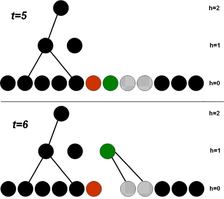
Figure 1: Two consecutive steps of dynamics at the initial stage ($t=5$ and $6$). One agent $n=1$ is promoted (green), and gains $\mu=2$ new followers (dashed nodes), and one agent is degraded to $h=0$ (red). In the given example the algorithm selected for degradation an agent from the bottom level.

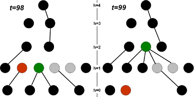
Figure 2: Two consecutive steps of dynamics at the stationary state ($t=98$ and $99$). One agent $n=1$ is promoted (green), and gains $\mu=2$ new followers (dashed nodes), one agent is degraded to $h=0$ (red).

As it was mentioned earlier, the proposed model is a network with a constant number of nodes. Albeit, the number of edges and hierarchy levels can change in time. Level $h=0$ is referred to as the ground level. Model dynamics is based on two processes: agents promotions (agents jump to a higher level) and their degradations (agents drop to the ground level). In every time step $n$ nodes are promoted and $d$ degraded. In both cases individual agents are chosen randomly from the set of nodes. When agent $i$ at level $h_{i}$ is promoted then $\mu$ new followers from the same level connect to it. Simultaneously, the promoted agent $i$ and its new followers lose connections with their current leaders. All of the followers of agent $i$, and the followers of its followers etc. increase their hierarchy levels by $1$. If at level $h_{i}$ there are less than $\mu+1$ nodes then another node (from different level) is chosen for promotion, until this condition is fulfilled. Degradation of agent $j$ means that it looses all its connections and is transferred to the lowest level $h=0$. In our model the connections between the nodes represent interactions which lead to the avalanches of promotions. Even if an agent is not directly promoted it can still increase its relevance resulting from the promotion of its leader (or leader’s leader etc.).

Initially, all agents are located at the ground level $h=0$. In the course of system evolution they change their placements and as a consequence the changes in occupation of hierarchy levels and in the overall structure of connections can be observed. Since edges can be added, rewired, and lost the created network is not fully connected. In further description we focus on statistical features of hierarchies in our system and a detailed analysis of topology will be neglected.

III Analytical and numerical results for balanced growth, $d=n$

III.1 Topology evolution

Emergence of new hierarchy levels is a consequence of two dynamical processes: nodes? promotions and degradations. Herein, we do not consider external forces. The interactions between agents are represented with links. In the course of time randomly chosen nodes change their hierarchy levels but size of the network is constant throughout. As was mentioned before in the initial time step $t=0$ all of the agents occupy level $h=0$ (ground state): $N_{0}(0)=N$. In every time step $t>0$ promotions and degradations are considered and number of nodes at levels $N_{h}(t)$ is changing. Also, the number of levels is subject to change.

Figure 3: Initial stage of the system evolution for $n=1$, $\mu=2$, $d=1$ and $N=1000$. A) Average hierarchy level $\left<h\right>(t)$. Line presents equation $nt/N$. B) Maximal hierarchy level $h_{max}(t)$. C) Total number of edges $E_{tot}(t)$. Line presents equation $n\mu t$. D) Number of nodes at the ground level $N_{0}(t)$. Line presents equation $N-nt$. Results of computer simulations are averaged over $Q=100$ realizations.

Figure 4: System evolution for $n=1$, $\mu=2$, $d=1$ and $N=1000$. A) Average hierarchy level $\left<h\right>(t)$. B) Maximal hierarchy level $h_{max}(t)$. C) Total number of edges $E_{tot}(t)$. D) Number of nodes at the ground level $N_{0}(t)$. Results of computer simulations are averaged over $Q=100$ realizations.

We are interested in eliciting qualitative and quantitative changes in hierarchical features of the system, i.e. average hierarchy level $\left<h\right>(t)$ and maximal level $h_{max}(t)$ (the height of the hierarchy). Additionally, to better understand the evolution process we examine changes of the total number of links $E_{tot}(t)$ and the number of agents at the ground state $N_{0}(t)$.

In the initial stage of evolution the system dynamics can be approximated as a process of $n$ promotions from the ground level to $h=1$. Degradations do not affect the system and are practically negligible (individuals chosen for degradations are located at $h=0$, see schematic picture in Fig. 1). It follows that the average hierarchy level equals $nt/N$ (see Fig. 3 A) ). A promoted agent gains $\mu$ followers and the number of links increase by $n\mu$ per step (see Fig. 3 C) ). Occupation of the lowest level decreases by $n$ of promoted nodes in every time step (see Fig. 3 D) ). This kind of behaviour is observed until $t<\frac{N}{n\left(\mu+1\right)}$ (Figs. 3 and 4). Thereafter, the network structure becomes increasingly complex making analytical description less trivial. Degradations influence system behaviour and promotions tend to be more collective, i.e. promotion of a node causes an ”avalanche” of promotions of its followers. The number of followers changes in time by taking new followers and switching leaders. After a longer period of time $t\gg N$ the system arrives at the stationary state, i.e. that network structure (averaged over a large number of realizations) is independent from time. Promotions and degradations balance themselves and there are no visible changes in network characteristics. The number of links, the number of nodes at the ground state, the average hierarchy level and the maximal hierarchy level are all constant. It is worth noticing that qualitatively the course of evolution is of universal character (it does not depend on system size $N$ if large enough number of nodes is fed into the system). The abovementioned quantities for different system sizes in the stationary state are presented in Fig. 5. Only maximal level $h_{max}$ grows logarithmically with $N$ (detailed discussion of this problem is presented in Section III.3). Our assumption that the existence of hierarchy level $h$ is equal to the observation of this level at least once effects that for a larger number of nodes there are bigger chances to observe higher levels. The occupation of these levels is minute and does not influence the value of the average hierarchy level.

Based on system behaviour in time, especially on the fact that for fixed values of parameters $n$, $\mu$, $d$ there are limited values of quantities describing the system, in the following part of the paper we focus on their analytical description.

Figure 5: System characteristics in the stationary state as a function of its size for $n=1$, $\mu=2$, $d=1$. A) Average hierarchy level $\left<h\right>(N)$. B) Maximal hierarchy level $h_{max}(N)$. Line presents Eq. (16). C) Total number of edges per node $E_{tot}/N(N)$. D) Fraction of nodes at the ground level $N_{0}/N(N)$. Results of computer simulations are averaged over $Q=500$ realizations and for every network for $N$ last steps of dynamics in the stationary state. Time of one realization is $T=10\cdot N$.

III.2 System in the stationary state

In this Section we focus on finding distribution of nodes at hierarchy levels $P_{h}$ in the stationary state. Since the number of links in the system and the number of nodes at the ground state are independent from time we can find the average number of followers per node in the whole system as

$$\kappa=\frac{E_{tot}}{N-N_{0}}.$$ (1)

When this quantity is observed locally then it equals $0$ for nodes at $h=0$ (these nodes cannot have followers), and we will assume that for higher levels ($h>0$) it does not depend on $h$. Numerical simulations show that this assumption is fulfilled for majority of levels. The number of followers is strictly related to the size of promotion avalanche $K$, i.e. the total number of indirectly promoted agents (except the chosen nodes). Value $K$ corresponds to the size of avalanche bak or mean local reaching centrality mones . The distribution of promotion avalanches $\Phi(K)$ is presented at Fig. 6. As one can observe, the probability decreases approximately exponentially with size of avalanche $K$. For higher $\mu$ we have observed a faster decrease. Since in the numerical data $\Phi(0)+\Phi(1)+\Phi(2)>0.9$, in our analytical treatment we neglected the interactions between hierarchy levels that are not in the nearest neighbourhood ($\neq h\pm 1$). The above approximation makes us possible to express changes of a number of nodes $N_{0}(t)$ at level $h=0$ by the following processes. During a single promotion event the occupation $N_{0}(t)$ increases by $1$ as a consequence of agent’s promotion from this level with probability $\frac{N_{0}(t)}{N}$ or by $\kappa$ due to promotion of agent from level $h=1$ with probability $\frac{N_{1}(t)}{N}$. On the other hand degradation of one agent from any level $h>0$ increases $N_{0}$ by $1$ with probability $\frac{N-N_{0}(t)}{N}$. The dynamics can be described by a simple rate equation

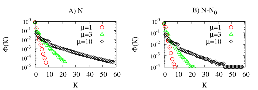
Figure 6: Promotions avalanche distributions $\Phi(K)$ for A) all nodes in the network and B) nodes at levels $h>0$. Computer simulations are performed for: $n=1$, $\mu=2$, $d=1$, $N=1000$ and are averaged over $Q=500$ realizations and for every network realization for $N$ of last steps of dynamics in the stationary state. Time of one realization is $T=10^{4}$.

$$N_{0}(t+1)=N_{0}(t)-n\frac{N_{0}(t)}{N}+d\frac{N-N_{0}(t)}{N}-n\kappa(t)\frac{N_{1}(t)}{N},$$ (2)

Similarly to the case where $h=0$ we can write rate equation for every $h>0$ taking into account promotions from levels $h-1$, $h$, $h+1$ and degradations from any $h$ as

$$N_{h}(t+1)=N_{h}(t)-d\frac{N_{h}(t)}{N}+n\frac{N_{h-1}(t)}{N}+$$ (3)

$$-n\frac{N_{h}(t)}{N}+n\kappa(t)\frac{N_{h}(t)}{N}-n\kappa(t)\frac{N_{h+1}(t)}{N}.$$

Let us define $\gamma=\frac{d}{n}$ as degradation ratio. Then Eqs. (2) and (III.2) in a stationary state can be written as follows

$$\gamma N-(\gamma+1)N_{0}-\kappa N_{1}=0,$$ (4)

$$\left(\gamma+1-\kappa\right)N_{h}-N_{h-1}+\kappa N_{h+1}=0.$$ (5)

Let us notice that Eq. (5) is a recurrence equation with expected solution

$$N_{h}=N_{0}\lambda^{h},$$ (6)

where $\lambda=\frac{N_{h+1}}{N_{h}}$ is a ratio of neighbouring levels occupancy and is independent from $h$ (similarly to quantity $\kappa$ this assumption is true for the majority of levels). The number of nodes in the system is constant and can be written as a sum

$$N=\sum_{h=0}^{h_{max}}N_{h}=N_{0}\sum_{h=0}^{h_{max}}\lambda^{h},$$ (7)

where $h_{max}$ is maximal hierarchy in the system. Assuming $h_{max}\gg 1$ we find

$$\frac{N_{0}}{N}\approx 1-\lambda$$ (8)

In the stationary state the number of lost and added links is equal, thus $E_{tot}=const$ (see Fig. 4). If we consider promotion of $n$ nodes and degradation of $d$ nodes at a time step we can write change of total number of links in the system as

$$\Delta E_{tot}=-n\kappa\lambda+n\mu\left(1-\kappa\lambda\right)-d\kappa\lambda-d\kappa\lambda=0.$$ (9)

Consecutive elements of the above equation correspond to the following processes:

$(i)$

$-n\kappa\lambda$ $\rightarrow$ promoted nodes lose connections with current leaders,

$(ii)$

$+n{\mu}\left(1-\kappa\lambda\right)$ $\rightarrow$ every promoted agent gains ${\mu}$ new followers, which lose links with their current leaders,

$(iii)$

$-d\kappa\lambda$ $\rightarrow$ degraded agents lose connection to their leaders,

$(iv)$

$-d\kappa\lambda$ $\rightarrow$ degraded agents from level $h>0$ (probability that agent is not at level $h=0$ is $\frac{N-N_{0}}{N}=\lambda$) lose links with their followers.

Taking into account Eqs. (4) -(8) after some algebra one can find analytical forms of characteristic system quantities $\kappa$, $\lambda$, $N_{0}/N$, $E_{tot}/N$.

$$\kappa({\mu},\gamma)=\mu\frac{2\mu+\gamma\mu+2\gamma^{2}+3\gamma+1}{\left(2\mu+1+2\gamma\right)\left(\mu+1+2\gamma\right)}$$ (10)

$$\lambda(\mu,\gamma)=\frac{2\mu+1+2\gamma}{2\mu+\gamma\mu+2\gamma^{2}+3\gamma+1}$$ (11)

$$\frac{N_{0}}{N}\left(\mu,\gamma\right)=\gamma\frac{\mu+1+2\gamma}{2\mu+\gamma\mu+2\gamma^{2}+3\gamma+1}$$ (12)

$$\frac{E_{tot}}{N}\left(\mu,\gamma\right)=\frac{\mu}{\mu+1+2\gamma}$$ (13)

Next, we put Eqs. (12) and (11) into Eq. (6) and define the probability of finding a node at level $h$ as $P_{h}=\frac{N_{h}}{N}$. Finally we arrive at

$$P_{h}=\frac{\gamma\left(\mu+1+2\gamma\right)}{2\mu+\gamma\mu+2\gamma^{2}+3\gamma+1}\left(\frac{2\mu+1+2\gamma}{2\mu+\gamma\mu+2\gamma^{2}+3\gamma+1}\right)^{h}.$$ (14)

The average hierarchy level can be approximated by the simple sum

$$\left<h\right>=\sum_{h=0}^{\infty}\left(h\cdot P_{h}\right)=\frac{2\mu+2\gamma+1}{\gamma\left(\mu+2\gamma+1\right)}.$$ (15)

Figure 7: System characteristics in the stationary state as a function of number of new followers $\mu$, for $n=1$, $d=1$ and $N=1000$. A) Average number of node followers $\kappa(\mu)$. Results of computer simulations put into Eq. (1) are presented with symbols; line presents Eq. (10). B) Ratio of the number of nodes at two neighbouring levels $\lambda(\mu)$. Line presents Eq. (11). Results of computer simulations are averaged over $Q=500$ realizations and for every network for last $N$ steps of dynamics in a stationary state. Time of one realizations is $T=10^{4}$.

Figure 8: Average number of node followers as a function of degradation ratio $\kappa(\gamma)$ for $\mu=2$ and $N=1000$. Results of computer simulations put into Eq. (1) are presented with symbols, line presents Eq. (10). Points corresponding to $\gamma>1$ are obtained for $n=1$ and $d>1$, $\gamma<1$ corresponds to $d=1$ and $n>1$. Results of computer simulations are averaged over $Q=500$ realizations and for every network for last $N$ steps of dynamics in stationary state. Time of one realizations is $T=10^{4}$.

Figure 9: System characteristics in the stationary state as a function of the number of new followers $\mu$, for $n=1$, $d=1$ and $N=1000$. Results of computer simulations are presented with symbols. A) Average hierarchy level $\left<h\right>$. Line presents Eq. (15). B) Maximal hierarchy level $h_{max}$. Line presents Eq. (16). C) Total number of edges per node $E_{tot}/N$. Line presents Eq. (13). D) Fraction of nodes at the ground level $N_{0}/N$. Line presents Eq. (12). Results of computer simulations are averaged over $Q=500$ realizations and for every network for last $N$ steps of dynamics in stationary state. Time of one realizations is $T=10^{4}$.

Figure 10: System characteristics in the stationary state as a function of degradation ratio $\gamma$ for $\mu=2$, $N=1000$. Results of computer simulations are presented with symbols. Points corresponding to $\gamma>1$ are obtained for $n=1$ and $d>1$, $\gamma<1$ corresponds to $d=1$ and $n>1$. A) Average hierarchy level $\left<h\right>$. Line presents Eq. (15). B) Maximal hierarchy level $h_{max}$. Line presents Eq. (16). C) Total number of edges per node $E_{tot}/N$. Line presents Eq. (13). D) Fraction of nodes at the ground level $N_{0}/N$. Line presents Eq. (12). Results of computer simulations are averaged over $Q=500$ realizations and for every network for last $N$ steps of dynamics in stationary state. Time of one realizations is $T=10^{4}$.

Figure 11: Distributions of nodes at hierarchy levels $P_{h}$ for different number of new followers $\mu$: A)$\mu=1$, B)$\mu=2$, C)$\mu=5$, D)$\mu=10$. Results of computer simulations for $n=1$, $d=1$ and $N=1000$ are presented by symbols, lines present Eq. (14). Results of computer simulations are averaged over $Q=500$ realizations and for every network for last $N$ steps of dynamics in stationary state. Time of one realizations is $T=10^{4}$.

Comparison of computer simulations and analytical expressions is presented at Figs 7 - 11.

One interesting observation is that the average number of followers $\kappa$ is very low even for large numbers of new followers $\mu$ (see Fig. 7 A) ), $\kappa<1$ for $\mu<5$. This effect is caused by the possibility of changing agent?s speaker in the course of promotion process. The quantity $\kappa$ is almost monotonically increasing with parameter $\gamma$ (Fig. 8). The ratio of a number of nodes at neighbouring levels increases with the number of new followers $\mu$ (with fixed $\gamma$, see Fig. 7 B) ). When the number of degradations is much smaller than the number of promotions, i.e. $\gamma\rightarrow 0$ the number of nodes at all levels is almost the same, i.e. $\lambda\rightarrow 1$. Larger number of promotions in comparison with degradations make system more heterogeneous. The fraction of nodes at the ground level $N_{0}/N$ decreases with $\mu$ (see Fig. 9 D) ) and increases with $\gamma$ (see Fig. 10 D) ). Contrary behaviour is observed with regard to the number of edges per node (see Figs 9 C) and 10 C) ). Large number of degradation results with a smaller number of links which leads to higher occupation at the ground level. Average hierarchy level increases with $\mu$ (see Fig. 9 A) ) and decreases with $\gamma$ (see Fig. 10 A) ). Distributions $P_{h}$ (Fig. 11) show faster decrease for higher $\mu$ we have observed faster decrease, wherein the differences between levels? occupations are bigger.

III.3 Maximal hierarchy level

During the computer simulations maximal hierarchy was defined as highest $h$ observed at least once during all steps and all realizations of the dynamics. What it means is that the said quantity can be regarded as a kind of fluctuation and its size tends to grow along $N$. In the stationary state we do not observe emergence of new levels. In accordance with dynamic rules we assume that a new level cannot emerge provided the occupation of existing maximal level is no greater than $\mu$ nodes. To find analytical form of $h_{max}$ we assumed that the average number of nodes at highest level should equal $\frac{\mu+1}{2}$. It corresponds to a situation when at maximal level there can be $N_{h_{max}}=1,2,\ldots,\mu$ agents and all these cases are possible with equal probability. Putting $P_{h_{max}}=\frac{\mu+1}{2N}$ into Eq. (6) one gets

$$h_{max}=\frac{\ln{\frac{\mu+1}{2N}}-\ln\left(1-\lambda\right)}{\ln\left(\lambda\right)}.$$ (16)

Results of the above equation and the results of computer simulations are shown at Figs 5 B), 9 B) and 10 B). Eq. 16 confirms logarithmic growth of $h_{max}$ with the system size $N$ (Fig. 5 B) ).

III.4 Critical degradation ratio

Thus far we have shown that for fixed system parameters ($\gamma=d/n$, $N$ and $\mu$) the system reaches a stationary state and a limited value of $h_{max}$. Naturally, one question to address is whether there is a critical value of degradation ratio $\gamma^{*}$, for which the growth of hierarchies will not be observed, i.e. $h_{max}=1$. This condition is equal to a situation when on average one agent can be found at levels $h>0$ ($N-1$ agents occupy the ground level, $h=0$)

$$N_{0}=N-1.$$ (17)

Taking into account the above conditions and Eqs. 11, 12, 14 we get

$$\gamma^{*}(\mu,N)=\frac{\sqrt{\mu^{2}-10\mu+12\mu N+\left(2N-1\right)^{2}}}{4}+$$ (18)

$$+\frac{2N-\mu-3}{4}\xrightarrow{\mu\ll N,N\rightarrow\infty}N.$$

Critical degradation ratio value is close to the number of nodes in the system, which means that even for high number of degradations (in comparison to the number of promotions) hierarchical structures will be created. Quantity $\gamma^{*}$ also increases with the number of new followers $\mu$.

IV Leaders without followers - individual promotions

So far, only collective promotions have been described, i.e. every promoted agent brought about promotion of its followers and the consecutive followers. How strongly this affects system behaviour is a question to be addressed below. To answer it we have performed numerical simulations and found analytical solution for a scenario when promoted agents do not have any followers, i.e. individual promotions are considered and $\mu=0$ thus $\kappa=0$ and $E_{tot}=0$. Then rate equations (2) and (III.2) loose elements with $\kappa$ and we can find analytical solution for $N_{0}(t)$

$$\frac{N_{0}(t)}{N}=\frac{1}{n+d}\exp(-\frac{n+d}{N}t)+\frac{d}{n+d}$$ (19)

Figure 12: Fraction of nodes at the ground level in time $N_{0}(t)/N$. Results of computer simulations for $n=1$, $\mu=0$, $d=1$ and $N=1000$ are presented with symbols, line presents Eq. (19). Results of computer simulations are averaged over $Q=500$ realizations.

When $t\rightarrow\infty$ the first term in Eq. 19 goes to zero and the stationary solution is only provided by the second element. It means that for individual promotions the occupation of levels is independent from the number of new followers. Similarly it is possible to get the formula for every next $N_{h}(t)$. The number of nodes at the ground level is higher in case of single promotions than it is for collective promotions (see Figs 4 D) and 12). This effect confirms that collective promotions produce steeper hierarchical systems.

Similarly to the case $\mu>0$ we can write stationary form of rate equations describing $N_{0}$ and $N_{h}$ and find the ratio between the number of nodes at neighbouring levels as

$$\lambda=\left(\gamma+1\right)^{-1}.$$ (20)

Now using Eq. (20) we can find the number of nodes at level $h$ as

$$\frac{N_{h}}{N}=\frac{\gamma}{\gamma+1}\left(\gamma+1\right)^{-h}.$$ (21)

Average hierarchy level for $\mu=0$ (using eqs (15) and (21)) is

$$\left<h\right>\left(\gamma\right)=\frac{1}{\gamma},$$ (22)

which is simply the ratio between the number of promoted nodes and the number of degraded ones.

One can see from (21) that for $\gamma\gg 1$ (the number of degradations is much higher than the number of promotions) occupation of level $h=0$ tends to $N$. In the opposite case, when $\gamma\ll 1$ (the number of degradations is negligible in comparison with the number of promotions) $N_{0}\rightarrow 0$. These results are in agreement with intuition. In close similarity to the previous Section we can find critical degradation ratio $\gamma^{*}$ above which hierarchies do not emerge

$$\gamma^{*}=N-1.$$ (23)

Figure 13: System characteristics in the stationary state as a function of degradation ratio $\gamma$ for $\mu=0$, $N=1000$. Results of computer simulations are presented with symbols. Points corresponding to $\gamma>1$ are obtained for $n=1$ and $d>1$, $\gamma<1$ correspond to $d=1$ and $n>1$. A) Average hierarchy level $\left<h\right>(\gamma)$. Line presents Eq. (22). B) Maximal hierarchy level $h_{max}(\gamma)$. Line presents Eq. (16). C) Fraction of nodes at the ground state $N_{0}/N$. Line presents Eq. (21). D) Ratio of number of nodes at two neighbouring levels $\lambda=\frac{N_{h+1}}{N_{h}}$. Line presents Eq. (20). Results of computer simulations are averaged over $Q=500$ realizations and for every network for last $N$ steps of dynamics in stationary state. Time of one realizations is $T=10^{4}$.

Results of performed computer simulations and theoretical treatment are shown at Fig.13. Qualitative behaviour of our system for $\mu=0$ is similar to previous results for the case $\mu>0$ (see Fig. 10). One can observe quantitative differences for both scenarios. When $\gamma=0.05$, the average hierarchy level $\left<h(\mu=0,\gamma=0.05)\right>\approx 20$, while $\left<h(\mu=2,\gamma=0.05)\right>\approx 37$. As it can be seen, there is almost double decline of the average hierarchy level when we consider the absence of followers in the system. Similar differences can be observed for the fraction of nodes at the ground level. In the case of $\mu=0$ and $\gamma=0.05$ at level $h=0$ there are $N_{0}\approx 0.05N$ agents, while for $\mu=2$ there are almost twice less ($\approx 0.028$). It shows that the process of hierarchy growth is more distinct when we consider interactions between individuals (links between nodes).

V Discussion and Conclusions

We have shown that the process of hierarchy growth in a simple bottom-up approach tends to a stationary state that is described by agents distribution decaying exponentially with the hierarchy level $h$ as $N_{h}\sim\lambda^{h}$ (where the scaling ratio $\lambda<1$). This ”equilibrium” takes place irrespective of consecutive ”perturbations” of the system through collective promotions and individual degradations. The finding is well documented by extensive numerical simulations that have been confirmed by analytical results based on the rate equation method. The picture reminds Boltzmann distribution of occupation of energy levels in one-dimensional quantum harmonic oscillator where the hierarchy level $h$ corresponds to the oscillator energy and $-\log(\lambda)$ corresponds to the inverse of system temperature.

The above mentioned stationary state occurs when the age of the system is much larger than the system size $t\gg N$. Then the average hierarchy level $\left<h\right>$, the number of links per agent $E_{tot}/N$, the fraction of nodes at the ground state $N_{0}/N$ are independent from the system size (provided it is large enough). The above observables rely on parameters tied up with system dynamics, i.e. the number of new followers $\mu$ and the effective degradation ratio defined as a ratio of number $d$ of degradations and number $n$ of promotions per time unit $\gamma=\frac{d}{n}$. The system size $N$ does influence however the maximal hierarchy level $h_{max}$ that increases logarithmically with $N$ although the occupation of $h_{max}$ is small and does not affect the value of $\left<h\right>$.

Stationary values of $\left<h\right>$, $h_{max}$ and $E_{tot}/N$, increase with $\mu$ and decrease with $\gamma$. Opposite behaviour is observed for $N_{0}/N$ while the average number of agent followers i.e. the system branching factor $\kappa$ is increasing with $\mu$ and is a non monotonous function of $\gamma$. It is intriguing that for $\gamma=1$ we need a big number of initial followers $\mu>5$ to have the final branching ratio $\kappa>1$. The scaling ratio $\lambda$ of agent distribution $N_{h}$ increases with the parameter $\mu$, i.e. a higher system temperature corresponds to a larger number of new followers of every promoted agent.

The hierarchy exists also when promoted agents do not gain followers and there are no links in the system ($\mu=0$). Then the scaling ratio of agent distribution is $\lambda=\left(1+\gamma\right)^{-1}$ and the average hierarchy level is $\left<h\right>=1/\gamma$. Since the last value is lower than for the case $\mu>0$ thus interactions between individuals represented by links and leading to collective promotions amplify the hierarchy growth.

In our previous work pre we considered models of growing hierarchical networks from the top to the bottom, where newcomers tried to situate themselves as close as possible to the highest level according to limited knowledge about current network structure. We showed that the availability of the information can limit the hierarchy growth. The considered here emergence scenario from the bottom to the top seems to be more robust, i.e. new levels do not appear in the system only if the ratio between the number of degradations $d$ and the number of promotions $n$ is close to the system size $N$.

- (1) D. Pumain, Hierarchy in Natural and Social Sciences (Springer, 2006).
- (2) H. Jeong, B. Tombor, R. Albert, Z. Oltvai, A.-L. Barabási, The large-scale organization of metabolic networks, Nature (London) 407, 651 (2000).
- (3) A. Wagner, D.A. Fell, The small world inside large metabolic networks, Proc. R. Soc. London Ser. B 268, 1803 (2001).
- (4) H. Jeong, S. Mason, A.-L. Barabási, Z.N. Oltvai, Lethality and centrality in protein networks, Nature (London) 411, 41 (2001).
- (5) A. Wagner, The Yeast Protein Interaction Network Evolves Rapidly and Contains Few Redundant Duplicate Genes, Mol. Biol. Evol. 18, 1283-1292 (2001).
- (6) D. van Dijk, G. Ertaylan, C.A.B. Boucher, P.M.A. Sloot, Identifying potential survival strategies of HIV-1 through virus-host protein interaction networks, BMC Systems Biology 4, 1 (2010).
- (7) M. Faloutsos, P. Faloutsos, C Faloutsos, On power-law relationships of the Internet topology, Comput. Commun. Rev. 29, 251 (1999).
- (8) R. Albert, H. Jeong, A.-L. Barabási, Diameter of the World-Wide Web Nature (London) 401, 130 (1999).
- (9) M.E.J. Newman, The structure of scientific collaboration networks Proc. Natl. Acad. Sci. U.S.A. 98, 404 (2001).
- (10) M.E.J. Newman, Scientific collaboration networks. I. Network construction and fundamental results, Phys. Rev. E 64, 016131 (2001).
- (11) A.-L. Barabási, H. Jeong, Z. Neda, E. Ravasz, A. Schubert, T. Vicsek, Evolution of the social network of scientific collaborations, Physica A 311, 590 (2002).
- (12) S. Mei, R. Quax, D.A.M.C. van de Vijver, Y. Zhu, P.M.A. Sloot, Increasing risk behaviour can outweigh the benefits of antiretroviral drug treatment on the HIV incidence among men-having-sex-with-men in Amsterdam, BMC Infectious Diseases 11, 118 (2011).
- (13) D. Lane, in Hierarchy in Natural and Social Sciences, edited by D. Pumain (Springer, 2006), Chap. 4.
- (14) M. Batty, in Hierarchy in Natural and Social Sciences, edited by D. Pumain (Springer, 2006), Chap. 6.
- (15) H. Simon, Proc. Am. Philosophical Society 106, 467-482 (1962).
- (16) H. Simon, in Hierarchy Theory: The Challenge of Complex Systems, edited by H. Pattee (George Braziller, New York, 1973).
- (17) P.W. Anderson, Science 177, 393-396 (1972).
- (18) J. Holland, Emergence: From Chaos to Order (Addison-Wesley, Redwood City, CA, 1998).
- (19) Nepusz T, Vicsek T, Hierarchical Self-Organization of Non-Cooperating Individuals. PLoS ONE 8(12) (2013).
- (20) E. Bonabeau, G. Theraulaz, J.-L. Deneubourg, Phase diagram of a model of self-organizing hierarchies, Physica A 217, 373-392 (1995).
- (21) K. Kacperski and J.A. Hołyst, Phase transitions and hysteresis in a cellular automata-based model of opinion formation, J. Stat. Phys. 84, 169-189 (1996).
- (22) K. Kacperski and J.A. Hołyst, Opinion formation model with strong leader and external impact: a mean field approach, Physica A 269, 511-526 (1999).
- (23) J.A. Hołyst, K. Kacperski and F. Schweitzer, Phase transitions in social impact models of opinion formation, Physica A, 285, 199-210 (2000).
- (24) A. Czaplicka, K. Suchecki, B. Miñano, M. Trias, J.A. Hołyst, Information slows down hierarchy emergence Phys. Rev. E. 89, 062810 (2014).
- (25) D. Stauffer, Phase transition in hierarchy model of Bonabeau, Int. J. Mod. Phys. C 14, 237 (2003).
- (26) K. Malarz, D. Stauffer, K. Kułakowski, Bonabeau model on fully connected graph, Eur. Phys. J. B 50, 195-198 (2006).
- (27) P. Bak, How nature works: the science of self organize criticality., Copernicus, New York (1996).
- (28) E. Mones, L. Vicsek, T. Vicsek, Hierarchy Measure for Complex Networks, PLoS ONE 7(3) (2012).