Network analysis of the COSMOS galaxy field

Abstract

The galaxy data provided by COSMOS survey for $1{{}^{\circ}}\times 1{{}^{\circ}}$ field of sky are analysed by methods of complex networks. Three galaxy samples (slices) with redshifts ranging within intervals 0.88$\div$0.91, 0.91$\div$0.94 and 0.94$\div$0.97 are studied as two-dimensional projections for the spatial distributions of galaxies. We construct networks and calculate network measures for each sample, in order to analyse the network similarity of different samples, distinguish various topological environments, and find associations between galaxy properties (colour index and stellar mass) and their topological environments.

Results indicate a high level of similarity between geometry and topology for different galaxy samples and no clear evidence of evolutionary trends in network measures. The distribution of local clustering coefficient $C$ manifests three modes which allow for discrimination between stand-alone singlets and dumbbells ($0\leq C\leq 0.1$), intermediately packed ($0.1<C<0.9$) and clique ($0.9\leq C\leq 1$) like galaxies.

Analysing astrophysical properties of galaxies (colour index and stellar masses), we show that distributions are similar in all slices, however weak evolutionary trends can also be seen across redshift slices. To specify different topological environments we have extracted selections of galaxies from each sample according to different modes of $C$ distribution. We have found statistically significant associations between evolutionary parameters of galaxies and selections of $C$: the distribution of stellar mass for galaxies with interim $C$ differ from the corresponding distributions for stand-alone and clique galaxies, and this difference holds for all redshift slices. The colour index realises somewhat different behaviour.

1 Introduction

The observable large-scale structure of the Universe appears to be rich in a variety of shapes and topological features, we can identify clusters, super clusters, voids, walls and filaments in it. Altogether they comprise the Cosmic Web, the term coined in Bond et al. (1996). Numerous approaches have been devised in an attempt to properly describe and analyse the geometry and topology of the Cosmic Web, see for example the recent studies (Cautun et al., 2014; Chen et al., 2015, 2016; Hahn, 2014; Leclercq et al., 2016; Lee & Yepes, 2016; Pace et al., 2015; Pranav et al., 2016; Ramachandra & Shandarin, 2016; Zhao et al., 2015; Libeskind et al., 2017).
Methods and approaches of network science, see (Albert & Barabási, 2002; Dorogovtsev & Mendes, 2003; Barrat et al., 2008; Newman, 2010; and references therein, ), have recently proliferated into various disciplines including cosmology, (Hong & Dey, 2015; Hong et al., 2016; Coutinho et al., 2016). Complex networks are believed to assist in solving various open problems of cosmology, e.g. clarify the impact of environment on galaxy evolution (Brouwer et al., 2016; Kuutma, Tamm & Tempel, 2017); quantify the geometry and topology of large scale structures; understand the formation of phase-space distribution of dark and luminous matter and thus reveal the nature and properties of dark matter and dark energy.
The aim of the present paper is to study of the observable Cosmic Web with the aid of complex networks, develop and validate a universal approach for extracting topological environments from the observational data, in order to investigate the relation between properties of a galaxy and its place in large-scale structures, such as clusters, voids, walls etc.

We follow the pioneering paper by Hong & Dey (2015) where three network measures of topological importance (degree centrality, closeness centrality and betweenness centrality) have been derived for one galaxy sample from the COSMOS catalogue Ilbert et al. (2013), different topological environments in the Cosmic Web have been selected and their relationship to evolutionary parameters has been estimated. This paper Hong & Dey (2015) in turn follows Scoville et al. (2013), where the same problem was addressed using “traditional” methods and the same data source.

In comparison with already existing methods developed for Cosmic Web analysis, network analysis has a number of potential benefits: (a) it is not built on some ad-hoc assumptions on the nature of the data, e.g. existence of a continuous density field; (b) it’s computationally effective in treating discrete data, as no density estimator or Hessian is computed; (c) it is capable of describing and quantifying the content of data at an adjustable level of detail and complexity, properly encoding information; (d) it’s equally applicable to results of simulations and real observational data, thus allowing for direct comparison between them; (e) it can go beyond the classification of environments as clusters or filaments, by providing a more holistic view on the topology of the multi-scale phenomenon of the Cosmic Web. Thus, network analysis can complement other methods and effectively integrate them into a framework capable of investigating the complexity of large-scale structures of the Universe.

Here, we extend network analysis to include several galaxy samples and compare constructed networks by introducing other network metrics of interest like: number of edges, mean node degree, size of the giant connected component, average path length and diameter, assortativity. Also, we advocate the usage of clustering coefficient as a measure of short-range order which provides a robust technique that can be applied to generate networks for real observational data and simulation outputs. Moreover, we assess the applicability, restrictions and accuracy of such a technique.

The paper is organised as follows. In Section 2 we describe the observational data, the methodology of network construction and analysis is summarised in Section 3. Section 4 is devoted to results and discussion. The conclusions to be found in Section 5.

2 COSMOS samples of galaxies

The COSMOS Collaboration is a grand astronomical endeavour which seeks to integrate data produced by a variety of space and ground-based telescopes. The survey is aimed at analysing galaxy evolution and designed to collect essentially all possible objects in the field of view, i.e. to be as deep as possible, meanwhile covering an area of celestial sphere large enough to mitigate for the influence of cosmic variance.

The datasets for exploration are driven from the catalogue built by Ilbert et al. (2013) on the base of UltraVISTA ultra-deep near-infrared survey, data release DR1 McCracken et al (2012). It includes directly observable quantities, such as celestial coordinates for galaxies and photometric magnitudes for a number of broad bands, as well as colour corrected for dust extinction, $M_{NUV}-M_{R}$. Moreover, the dataset includes indirect estimations obtained by fitting models to photometric data Ilbert et al. (2013): most important is $z$, the redshifts for galaxies; basic galaxy classification according to colour – quiescent or star-forming; and other physical parameters of galaxies, e.g. stellar mass.

This catalogue was built for studying the mass assembly of galaxies Ilbert et al. (2013), used for exploring the evolution of galaxies and their environments in Scoville et al. (2013), as well as for constructing complex networks Hong & Dey (2015). Thus, this data set could be considered as a standard for benchmarking different kinds of large-scale structure analyses.

To achieve the goals of this study, we require independent samples of galaxies, meaning each sample should contain a unique set of galaxies. The samples should also approximately represent the same statistical population, to ensure comparisons statistically viable. As the survey covers quite a modest area of celestial sphere, the optimal region to be chosen lies in the centre of surveyed area where the right ascension (R.A.) spans the range $149\overset{{}^{\circ}}{.}\!4\div 159\overset{{}^{\circ}}{.}\!4$ and declination (Decl.) is in the range $1\overset{{}^{\circ}}{.}\!7\div 2\overset{{}^{\circ}}{.}\!7$.

The samples of galaxies are derived from the data set considering neighbouring ranges of redshift: $0.88\leq z<0.91$, $0.91\leq z\leq 0.94$ and $0.94<z\leq 0.97$, to be referred hereafter as $z_{1}$, $z_{2}$ and $z_{3}$ respectively. By this choice we extend the data analysed by Hong & Dey (2015) for redshift $z_{2}$ to include neighbouring redshift slices $z_{1}$ and $z_{3}$. Such an extension should minimise the influence of selection effects meanwhile providing large enough populations of different types of galaxies, including a high proportion of early-type (red) galaxies. Also, the central slice reproduces the one used in Scoville et al. (2013), where it was shown that when $z>1$ the relation of galaxy properties within a local environment abruptly diminishes.

The elaborated analysis of multi-band photometry data estimates the redshifts of galaxies to a high degree of accuracy (at 1% level). The thickness of slicing (redshift intervals $\Delta z$) is chosen to be comparable to the errors in $z$ and to ensure a large enough sample of galaxies to make statistical methods meaningful.

For the standard $\Lambda$CDM cosmology with $H_{0}$=70 km/s/Mpc and $\Omega_{\Lambda}=0.7$, a one degree distance on celestial sphere at $z=0.91$ corresponds to a distance of $\approx 54$ Mpc. Whilst the redshift interval $\Delta z=0.03$ corresponds to a spatial thickness of $\approx 76$ Mpc in comoving spatial coordinates. Despite the progress made in redshift determination, its accuracy is still insufficient to allow for three-dimensional spatial analysis. Thus, we analyse the each redshift as a two-dimensional projection of celestial sphere. This projection brings about some additional systematic bias and noise distorting the cosmic network. A more detailed discussion of such effects for density estimations can be found in Scoville et al. (2013).

Given the above mentioned restrictions of the data set, we still believe the data is good enough for answering the major questions at hand and validating the approach. The forthcoming releases of COSMOS and other extragalactic surveys can potentially mitigate or even remove such restrictions.

3 Methods of network analysis

3.1 Network construction

Contrary to the data coming from computer science, industrial databases and social networks, the data in cosmology are inherently non-networked and contains a substantial amount of noise. Hence, a graph (network) must be constructed from the data set (catalogue) using appropriate criteria and methodology, and preferably without losing relevant information. Such a procedure is equivalent to the transformation of data from an unstructured representation to a structured network representation (nodes and edges).
Thus, the task is to encode as much information of interest as possible, in this case the existence of structure over a random distribution of galaxies
There is no universal technique to construct a network for this kind of data, however the major steps to consider are the following: (i) Capture similarity between data points; (ii) Adopt some rules based on a similarity function for establishing the links between data points; (iii) Implement some criteria to judge whether the network is properly built, analogous to a “goodness-of-fit” procedure for approximation.

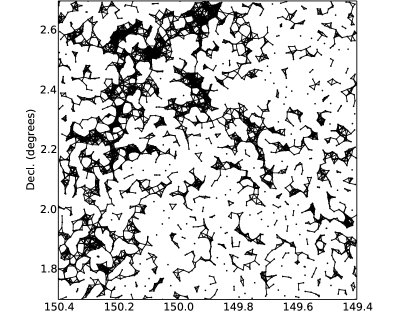
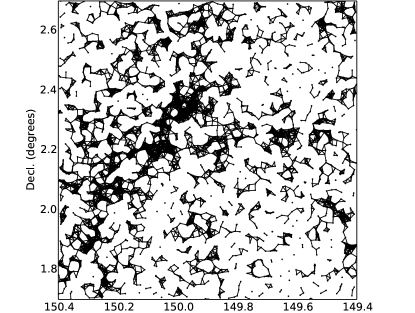
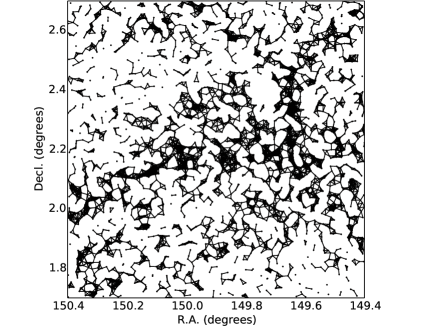
Figure 1: Complex networks constructed on the base of the redshift slices $0.88\leq z_{1}<0.91$, $0.91\leq z_{2}\leq 0.94$, and $0.94<z_{3}\leq 0.97$ (from top to bottom) from the COSMOS field using linking length of $0\overset{{}^{\circ}}{.}0216$. The middle figure recovers network that formerly obtained in Hong & Dey (2015).

Different techniques for constructing complex networks from a galaxy survey are discussed in Coutinho et al. (2016) on the basis of Illustris cosmological simulation, and it was shown that proximity is the most relevant similarity criterion for galaxy property studies. So, in this paper we apply a similarity parameter of proximity, called “linking-length”.
Here, an undirected network is constructed by generating edges between nodes, if and only if, the Euclidean distance between two nodes is less or equal to the prescribed linking-length, which is fixed. This simple recipe for analysing clustering was used for decades as “top-hat filtering” (Bardeen et al., 1986) and is closely related to the “friend-of-friend” algorithm (Press & Davis, 1982), used for the study of large-scale structures. In the context of unsupervised machine learning, the same approach is applied in density-based data clustering algorithms, like DBSCAN or OPTICS (Ester et al., 1997; Ankerst et al., 1999) as an $\varepsilon$-radius method.
So, hereafter a fixed linking length is predefined to be equal to $0\overset{{}^{\circ}}{.}0216$, this corresponds to a linear scale of 1.2 Mpc in the standard $\Lambda$CDM cosmology. This value was derived in Hong & Dey (2015) from particular Poissonian distribution of node degree, the closest to the observed one in the dataset.
Such a method is proven to be robust to noise, albeit it is claimed in Hong & Dey (2015) to not be universal, i.e. different samples would require different linking length. Here, we implement a goodness-of-fit measure based on the detection of a large connected cluster, or “giant component”, which is an indication of structure in the network. Also, the network should not be over-connected, or in other words it should be as sparse as possible in order to accurately reflect the relations between the nodes, and moreover be robust to noise.
Here, we investigate three cosmic networks constructed for the different redshift slices using the same linking length calculated for central slice (see also section 4.4). This allows to have consistency between samples and enables comparison and tracking differences across samples. As the outcome does not depend critically on precise value of linking length and redshift slices are adjacent such simplification does not introduce bias. In Fig.1 we show the cosmic networks generated using this prescribed linking length $l$ for each redshift slice. In the remainder of this section we will introduce the main metrics used in network science to quantify different features.

3.2 Network Metrics

One of the remarkable features of most complex networks is their heterogeneity. It leads to many unusual properties within networks. Below, we will introduce some characteristics that will be used to quantify network properties.

3.2.1 Size

The network is globally described by the numbers of nodes and edges, $n$ and $m$ respectively. For the connected part of a network, there is always a path between any pair of nodes $i$ and $j$. The shortest path length $\ell_{ij}$ between two nodes $i$ and $j$ can then be described as the shortest route in terms of number of steps to go from $i$ to $j$. The average path length $\langle\ell\rangle$ is then the average number of steps along the shortest path for all possible pairs of nodes belonging to the connected part of the network. It gives a measure of how closely related nodes are to each other. Below, we will calculate path lengths along the largest connected cluster of the network (Giant Connected Component, GCC).

The equation used to compute this quantity is:

$$\langle\ell\rangle=\frac{2}{g(g-1)}\sum_{i\neq j\epsilon GCC}\ell_{ij},$$ (1)

where $g$ is the total number of nodes in GCC, $\ell_{ij}$ is the shortest path between nodes $i$ and $j$, and the summation is performed over all nodes belonging to the GCC.

This can then be compared with the average path length for a classical Erdös-Rényi random network $\langle\ell_{r}\rangle$ (Erdos & Rényi, 1960) of the same size, where links are randomly assigned between nodes. Fronczak et al. (2004) have found it to be:

$$\langle\ell_{r}\rangle=\frac{\ln(g)-\alpha}{\ln(\langle k\rangle)+0.5},$$ (2)

where $\alpha\approx 0.5772$ is the Euler-Mascherroni constant (Weisstein, 2002) and $\langle k\rangle$ is the mean node degree defined in 3.2.2.

Another quantity that can be used to characterise the extent of a network is the longest shortest path between any two nodes, sometimes called the diameter of network, $D$. This path may provide an elegant description of the “back-bone” of the largest cluster in the cosmic network. In Table 1 we list the quantities $n$, $m$, $\langle\ell\rangle$, $\langle\ell_{r}\rangle$, $D$ and $g$ determined for all redshift slices. Percentages in brackets next to values of $D$ and $g$ indicate the portion of nodes belonging to the GCC.

3.2.2 Centralities

The importance of different nodes in a network can be determined by their centralities. For one of the COSMOS galaxy samples, $z_{2}$, the centralities of nodes have already been considered by Hong & Dey (2015). Here, besides calculating centralities for two more neighbouring redshift slices we evaluate not only their point estimates but also assess their distributions. In turn, this will allow us to compare galaxy samples in order to investigate how these metrics differ in other redshift slices. The centralities we consider are Degree, Betweenness and Closeness, see Brandes (2001) and definitions below.

The degree centrality provides information on the connectivity of a network within a localised area:

$$C_{d}(j)=\frac{k_{j}}{n-1},$$ (3)

where $n$ is the number of nodes in the network and $k_{j}$ is the degree (number of links adjacent) of node $j$, determined in terms of an adjacency matrix $\hat{A}$ as follows:

$$k_{j}=\sum_{i}A_{ij}\,,$$ (4)

here and below, when not explicitly specified, the summations indices span the entire network. For a network of $n$ nodes, $\hat{A}$ is an $n\times n$ matrix with elements $A_{ij}=1$ if there is a link between nodes $i$ and $j$ and $A_{ij}=0$ otherwise. Table 1 gives the mean values $\langle k\rangle$, $C_{d}$ and their standard deviations and standard errors (in brackets) for each network.

The betweenness centrality defines how important a node is in terms of connecting other nodes via shortest path lengths:

$$C_{b}(j)=\sum_{s,t(s\neq t\neq j)}\frac{\sigma_{st}(j)}{\sigma_{st}},$$ (5)

where $\sigma_{st}$ is the number of shortest paths between nodes $s$ and $t$ and $\sigma_{st}(j)$ is the number of shortest paths between nodes $s$ and $t$ that go through $j$.

The closeness centrality reveals how central a node is in the network. Within any sub-connected component $\mathcal{F}$ of $f$ nodes it is defined as:

$$C_{c}(j)=\frac{f-1}{n-1}\frac{f-1}{\sum_{t\epsilon\mathcal{F}}\ell_{jt}},$$ (6)

If the network is disconnected, as is the case for our networks, the first term will act to normalise the centralities for each fully connected subcomponent.

3.2.3 Correlations

Correlations within networks can be investigated using different techniques, implying both global and local characteristics. The Clustering coefficient of a network, in comparison with it random counterpart, can aid in quantifying the existence of structure within the local vicinity of a given galaxy and thus estimate its topological environment.

Local correlation is estimated by determining the clustering coefficient of an individual node:

$$C(j)=\frac{2y_{j}}{k_{j}(k_{j}-1)},$$ (7)

where $k_{j}\geq 2$ is degree of node $j$ and $y_{j}$ is the number of links between neighbouring nodes of node $j$. When $k_{j}<2$, then $C_{j}=0$ by definition. Averaging over all nodes in the network yields a mean clustering coefficient for the whole network, $C=\frac{1}{n}\sum_{i=1}^{n}C(i)$, the global characteristic of the network.

Table 1: Network metrics for three galaxy samples at different redshift, $z_{1}$, $z_{2}$, and $z_{3}$, along with mean values for colour index and stellar masses. Here, $n$ is number of nodes, $m$ is number of edges; $\langle\ell\rangle$, $\langle\ell_{r}\rangle$ are mean shortest path of GCC for real and random networks accordingly; $g$ is number of nodes and $D$ is diameter (maximal shortest path length) in the GCC; $k$ is node degree; $C_{d}$, $C_{b}$ are the degree and betweenness centralities; $C_{c1}$, $C_{c2}$ are closeness centralities for the distribution of fragmented clusters and GCC; $C$, $C_{r}$ are the mean clustering coefficients for real and random networks accordingly; $r$ is assortativity. The $Colour_{1}$ and $Colour_{2}$ are mean colour indexes for both modes of bimodal distribution, as shown in Fig. 7; $\log\,M_{stellar}$ is the logarithm of mean stellar mass (in units of solar one). Where it is applicable, in brackets the standard deviation ($\sigma$) and standard error (SE), or percentages to indicate the portion of nodes involved in particular component are given.

	0.88$\leq z<$0.91	0.91$\leq z\leq$0.94	0.94$<z\leq$0.97
	Mean  [$1\sigma$, SE]	Mean  [$1\sigma$, SE]	Mean  [$1\sigma$, SE]
$n$	3318	3678	3606
$m$	11747	14317	12206
$\langle\ell\rangle$	37.53	33.6	39.87
$\langle\ell_{r}\rangle$	3.06	3.00	3.12
$g$	2079  [63%]	2369  [64%]	2828  [78%]
$D$	116  [3.5%]	113  [3.1%]	117  [3%]
$k$	7.08  [5.02, 0.087]	7.79  [5.68, 0.093]	6.77  [4.36, 0.071]
$C_{d}$	0.0021  [0.0015, 0.00003]	0.0021  [0.0015, 0.00003]	0.0019  [0.0012, 0.00002]
$C_{b}$	0.0045  [0.014, 0.00023]	0.0037  [0.0097, 0.00016]	0.0066  [0.016, 0.00026]
$C_{c1}$	0.0019  [0.00012, 0.000033]	0.0028  [0.0018, 0.000029]	0.0018  [0.0013, 0.000047]
$C_{c2}$	0.018  [0.0041, 0.000090]	0.021  [0.0052, 0.000086]	0.021  [0.0052, 0.000097]
$C$	0.604  [0.263, 0.0048]	0.612  [0.261, 0.0043]	0.603  [0.264, 0.0044]
$C_{r}$	0.0021	0.0021	0.0019
$r$	0.85	0.86	0.80
$Colour_{1}$	0.64  [0.66, 0.012]	0.63  [0.68, 0.012]	0.61  [0.67, 0.012]
$Colour_{2}$	4.02  [0.54, 0.033]	4.20  [0.61, 0.032]	4.13  [0.66, 0.036]
$\log\,M_{stellar}$	9.29  [0.67, 0.012]	9.50  [0.69, 0.011]	9.44  [0.66, 0.011]

To this end, to determine how strongly correlated a particular network is, we can compare the $C$ with $C_{r}$, where $C_{r}$ is clustering coefficient for a Erdös-Rényi random network of the same size. Random networks are characterised by low values of $C_{r}$ and $\langle\ell_{r}\rangle$. So, if $C$ substantially exceeds $C_{r}$ this indicates that the network is highly correlated meaning that links in this network tend to be highly clustered together. The value of $C_{r}$ is calculated by simply considering $C_{r}=\langle k\rangle/n$.

Another useful estimator for node correlations is assortativity, $r$ which is usually used to investigate whether nodes of a similar degree tend to be linked together. This is similar to the Pearson correlation coefficient:

$$r=\sum_{i,j}\frac{A_{ij}(k_{i}-E[k])(k_{j}-E[k])}{E[k^{2}-E[k]^{2}},$$ (8)

where $A_{ij}$ is the adjacency matrix elements and $k_{i}$ and $k_{j}$ are the degrees of node $i$ and $j$ respectively, $E[k]$ is the mean node degree, $\langle k\rangle$, and $E[k^{2}]-E[k]^{2}$ is the mean variance of the node degree.

Thus, with complex networks we can analyse the structure in a galaxy sample as a whole and in more detail. In particular, extend analysis beyond the local density and quantify short-range anisotropy of the distribution by clustering coefficient. Furthermore, we can compare different samples, retrieving important information which could not previously be revealed via existing methods. In the following section we apply network metrics to classify topological environments. Moreover, the application of complex networks to the Cosmic Web analysis places the research into a more general context of complex systems thus creating opportunities to search for analogies between different phenomena that occur in systems of interacting agents of various nature.

4 Results and Discussion

Our results for different network metrics are listed in Table. 1, the columns represent three networks visualised in Fig. 1. As it was already discussed at the end of Section 3.1, we use the same linking length for all redshift slices to enable a comparative analysis and reduce undue bias.

In Table. 1 we can see that unique, yet similar samples of galaxies, produce networks with resembling characteristics. This serves as confirmation that we have a robust network generation method which generates a network with sufficient structure and relevant information. Meanwhile, such comparisons also point to the unbiasedness of the network generation method that exhibits sufficient sensitivity in detecting structure within galaxy distributions.

By comparing the average clustering coefficients $C$ and average path lengths $\langle\ell\rangle$ with their random counterparts $C_{r}$ and $\langle\ell_{r}\rangle$, we can see that generated networks are similarly, highly correlated networks, with evident regular structures within their GCCs. The GCC is analogous to the super cluster in a network and the diameter $D$ is analogous to the spine of the largest cluster. From Table 1 we see that all networks have slightly different GCCs with similar spines. This would indicate a variance in largest cluster size between networks with $z_{3}$ having the largest cluster and $z_{1}$ the smallest. Present analysis does not exclude the possibility that all three GCCs found for slices $z_{1}$, $z_{2}$ and $z_{3}$ belong to a single extended structure.

Figure 2: The statistical distributions (histograms with density plots) of degree centrality $C_{d}$ and clustering coefficient for three ranges of $z$ from left to right: $0.88\leq z_{1}<0.91$, $0.91\leq z_{2}\leq 0.94$, and $0.94<z_{3}\leq 0.97$.

We have computed the centrality measures for betweenness, closeness and degree, which Hong & Dey (2015) consider in their paper, and estimated their standard errors for three galaxy samples $z_{1}$, $z_{2}$ and $z_{3}$. The distributions for centralities are summarised in Table 1 and the distributions for degree centrality is shown in Fig.2.

4.1 Degree centrality

The degree centrality $C_{d}$ characterises the distribution of node degree in a network, so the mean of such a distribution directly relates to average degree $\langle k\rangle$. From Table 1 we can see that they are fairly similar with values of $7.08$, $7.79$ and $6.77$ for increasing values of redshift. On inspection of Fig. 2 (top row), the distributions on node centrality seem Poissonian in nature for all redshift slices, with $z_{1}$ and $z_{2}$ slices having more extended tails in comparison with $z_{3}$. This indicates that $z_{1}$ and $z_{2}$ have some really tightly packed galaxies within clusters whereas in $z_{3}$ the distances between galaxies are more evenly distributed within the clusters.

4.2 Betweenness centrality

The betweenness centrality $C_{b}$ measures the importance of a node in terms of maintaining connections between other nodes. In other words, a node that is involved in a larger number of shortest paths will be more important with respect to betweenness. Nodes which join two large components/clusters together will also have a high betweenness centrality. This is because many nodes exist in either of the two large clusters and hence many paths will have to traverse through these joining nodes. This would not be the case if one of the clusters was small and the other large. By this definition galaxies linking two larger clusters will display high betweenness centrality.
As it turns out from the analysis, the distribution of the betweeness centrality is negatively skewed indicating a fewer number of high betweenness nodes. The galaxies with high betweeness might be classified in astrophysical terms as filaments which join larger clusters together. Fig. 3 depicts how galaxies with betweenness centrality greater then $0.002$ (shown by red squares) represent only a small portion of the galaxies and how they all tend to be galaxies that form paths between larger clusters.

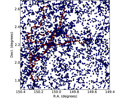
Figure 3: Galaxies in $z_{2}$-slice with betweenness centrality greater than $0.02$ are red squares and galaxies with lower value are denoted by blue circles.

4.3 Closeness centrality

We find that the distribution of closeness centrality $C_{c}$ is apparently bimodal with two peaks centered about the values $C_{c1}\approx 0.002$ and $C_{c2}\approx 0.02$. They are characterised by different widths, leading in turn to different variance of the distributions (see Table 1).

As it follows from a thorough analysis of the data, the population of galaxies that belong to the second peak corresponds to the largest connected component of the network (GCC). In turn, the nodes in the centre of the GCC are characterised by shorter distances to the rest of the nodes, leading by Eq. ($4$) to larger values of $C_{c}$. The periphery nodes are characterised by larger distances to the rest of the nodes, therefore they have smaller values of $C_{c}$.

In a similar way, one can identify the population of galaxies that give rise to the first peak in the $C_{c}$ distribution. These are the galaxies that belong to the smaller clusters, that are not attached to the GCC. Here, the central nodes of the clusters correspond to the right wing of the first peak and the periphery nodes are those contributing to the left wing. The possibility to find two distinct populations in the distribution is caused by the difference in sizes of the GCC and that of the rest of the network. The larger the difference, the more distinct the peaks. Indeed, as one can see from Table 1, the largest size of GCC ($78\%$) is find for the redshift interval $z_{3}$. This which corresponds to the case where the gap between the two peaks is most pronounced.

4.4 Clustering coefficient

As it follows from Eq. (7), the clustering coefficient $C(j)$ counts the ratio of triangles of connected nodes to all possible triples in a given cluster. In this way, the clustering coefficient is a useful measure for the correlation on a local level or short-range correlation. It provides information on elementary substructures (patterns) that appear in the network. In Table 1 observing clustering coefficient, one can see the presence of pervasive pattern-groups of tightly connected galaxies on different sites (see also Fig. 1) since the high values of average clustering coefficient are obtained for all redshifts slices.

Before continuing the discussion about the actual properties of $C$ for the networks under consideration, let us return back to the origins of network construction. As it was mentioned in Section 3.1, the choice of linking length $l$ is crucial in defining the network topology, and it appears to be particularly important with respect to correlation. Indeed, for a small $l$ the network is just a set of disconnected nodes and therefore $C=0$, while as it follows from Eq. (7) for large $l$ one arrives at the complete graph where $C=1$. In Fig. 4 we illustrate this by plotting $C$ as a function of $l$ for all redshift slices. One can see that $l=0\overset{{}^{\circ}}{.}0216$ chosen to construct Fig. 1 correspond to $C_{1}=0.604$, $C_{2}=0.612$, $C_{3}=0.603$ at $z_{1}$, $z_{2}$ and $z_{3}$ accordingly. So, this value of $l$ appears to be optimal as shown first in Hong & Dey (2015) and further supported by our analysis.

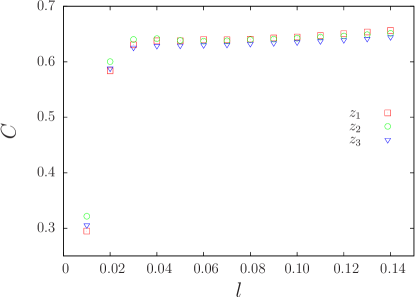
Figure 4: Clustering coefficient $C$ for all three redshift slices as a function of linking length $l$.

The local clustering of each node can also be considered in an effort to help construct robust methods of defining substructures within the cosmic network, or, for making selections to represent certain type of environment. Histograms for clustering coefficient in Fig. 2 depict complex discrete distributions with three main peaks at $0$, $0.66$ and $1$. In most cases galaxies with clustering coefficient $C_{i}<0.1$ have less then two neighbours, so they are located in sparse environments, where mean distance between galaxies is larger than the linking length. This selection can be called “stand-alone” galaxies represented by singlets and dumbbells residing mostly in sparse regions. The nodes with clustering coefficient ranging in $0.1\div 0.9$ indicate galaxies that are intermediately packed next to one another. Galaxies with a clustering coefficient larger than $0.9$ tend to highlight small clusters, or in other words participate in some “cliques”. Thus, we make three selections of galaxies, and analyse them below with regard to galaxy properties.

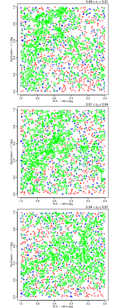
Figure 5: Galaxies from different selections marked according to their clustering coefficient. Red squares denote the “stand-alone” galaxies, green circles denote the galaxies with interim values of clustering coefficient, and small “cliques” are denoted by blue crosses.

In Fig. 5 three selections of galaxies are mapped onto spatial distributions, for each of three redshift slices. It is noticeable, that nodes within denser clusters do not necessarily exhibit higher clustering coefficient than their sparser counterparts. The main reason is the fixed linking length. For example, in these large clusters node $i$ will link to all nodes within prescribed linking length including node $j$ on the edge of linking length. However, as the linking length is smaller than the size of cluster, node $j$ will link to other nodes in this cluster which are unreachable for node $i$ (not all neighbours of $j$ will be linked to node $i$). Thus, counter intuitively, rather smaller clustering coefficients are seen among highly clustered galaxies, and clustering coefficient takes the highest values in smaller clusters at the edges of voids.

4.5 Average path length

The evaluation of average path length makes sense only for the giant connected component, because disconnected nodes will have no paths between them, which mathematically leads to infinite lengths. According to Table 1, $\langle\ell\rangle$ ranges between $33$ and $40$ for different slices, to be compared with the $\langle\ell_{r}\rangle$ of a random network of the same size.

In network theory significant amounts of attention have been paid to the idea of small worldedness (Watts and Strogatz, 1998): a network can be both highly correlated on a local level (i.e. nearest neighbour level) and exhibit relatively small $\langle\ell\rangle$ at the same time. When $C$ of a network exceeds randomly expected, $C\gg C_{r}$ and $\langle\ell\rangle$ is close or smaller than randomly expected, $\langle\ell\rangle\lesssim\langle\ell_{r}\rangle$, then a network is said to be small world in nature.

The cosmic networks do not display small world characteristics. All three networks satisfy the first condition of small worldedness in that they are far more correlated then randomly expected. However, these networks fail on the second condition in that $\langle\ell\rangle$ are all much larger than randomly expected and so can not be considered to be small world in nature. Therefore, the cosmic network is a large world in this context. This could well be a result of the constraint that is imposed by linking length, as this does restrict galaxies outside a certain distance from being linked and could be a contributing factor in why the network is a large world.

4.6 Assortativity

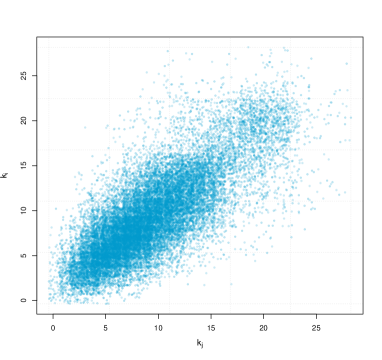
Figure 6: Scatter plot for degrees of connected nodes: $k_{i}$ and $k_{j}$ for the $z_{2}$ redshift slice.

For a disassortative network the value of $r$, Eq. (8), is negative indicating that nodes of low degree tend to associate with nodes of high degree. In turn when this value is positive this indicates an assortative network where nodes of similar degree link with one another. Fig. 6 provides a qualitative perspective where it can be clearly seen that the cosmic network displays positive correlation and this can be further confirmed quantitatively in Table 1 with $r$ for all redshifts being $\geq 0.80$. This indicates that in the cosmic network galaxies with a similar number of links tend to be connected to one another.

4.7 Astrophysical quantities vs topology

Figure 7: The statistical distributions of galaxy parameters: colour index and stellar mass for redshift slice $0.91\leq z_{2}\leq 0.94$.

Another goal of this research is to investigate how galaxy properties (hereafter the stellar mass and colour index) relate to the topological environment of galaxies (hereafter topological refers to selections according to clustering coefficient). The relationship between galaxy properties and network centrality measures have been considered by Hong & Dey (2015) for the $z_{2}$ slice. Here we take a different approach, based on clustering coefficient, and apply it to three samples of galaxies.

Before embarking into the analysis, we need to address a number of the limitations caused by the nature of the data. The exploration of clustering coefficient (bottom panel of Fig. 2) reveals its discrete and highly non-uniform distribution, meanwhile the astrophysical parameters are continuous variables with non-trivial distributions (especially colour index, see Fig. 7). Given that parametrical methods for multivariate analysis e.g. correlation analysis, are definitely inapplicable, and even though the application of non-parametrical methods cannot ensure feasible results we are left these methods to apply.

Of course, we can seek for trends by analysing general differences between distributions in samples, for instance by comparing their means and standard deviations, as in Table 1. However, the statistical significance of such differences is unknown.

The distributions of variables can be compared by means of non-parametric methods based on empirical distribution function (two-sample tests). At some confidence level, null hypothesis significance testings estimate $p$-values to be used for rejecting the null hypothesis, in this case that both selections are sampled from the same population. Note, that such tests result in binary answers (yes/no), seek to reject the null hypothesis, and should be taken with a grain of salt since they assume the univariate nature of variables.

Usually the Kolmogorov-Smirnov test (Kolmogorov, 1933; Smirnov, 1948) is used as a non-parametric test, as in Hong & Dey (2015). Although this test is universal tool, it has a number of limitations, and should be cross-validated by other approaches, like Anderson-Darling (Anderson & Darling, 1954) or Mann-Whitney-Wilcoxon (Mann & Whitney, 1947; Wilcoxon, 1945) tests.

4.7.1 Distributions of galaxy parameters

We first analyse distributions for colour index and stellar mass (Fig 7), the means and standard deviations are included in Table 1. The Hartigans’ dip test (Hartigan & Hartigan, 1985) proves that bimodalities in the colour distributions are statistically significant: the null hypothesis of unimodality is rejected with $p$-value $<2.2\cdot 10^{-16}$. The different heights of the peaks in histogram imply heterogeneity of the data set, which may be drawn from different populations.

With respect to colour index, non-parametric tests consistently indicate the following: the hypothesis of a common distribution is strongly rejected when comparing $z_{1}$ and $z_{3}$ samples, mildly rejected for $z_{1}$ and $z_{2}$ samples, and mildly accepted for $z_{2}$ and $z_{3}$ samples. Therefore, the tests have revealed a weak but still significant evolutionary trend for colour index over redshifts span.

Although the shape of distribution for stellar mass is simpler, two-sample tests for stellar mass detect significant distinctions over redshifts for all pair-wise comparisons except in the case of $z_{2}$ vs $z_{3}$. Note that colour index is derived directly from observed photometric measurements. Meanwhile, the stellar mass of galaxies is computed from the same photometric data using approximations and elaborate modeling of spectral energy distributions (SED).

Table 2: The results of Anderson-Darling tests ($p$-values) for colour and stellar mass distributions for different clustering coefficients selections: I $C=0$; II $0<C<1$; III $C=1$. The critical $p$-value equals 0.05.

	Colour			Stellar Mass
	$z_{1}$	$z_{2}$	$z_{3}$	$z_{1}$	$z_{2}$	$z_{3}$
I vs II	0.062	0.018	0.31	5$\cdot 10^{-6}$	0.0048	0.00023
II vs III	0.29	0.025	0.37	0.0032	0.0018	0.014
I vs III	0.74	0.79	0.49	0.19	0.91	0.18

4.7.2 Selections by clustering coefficient

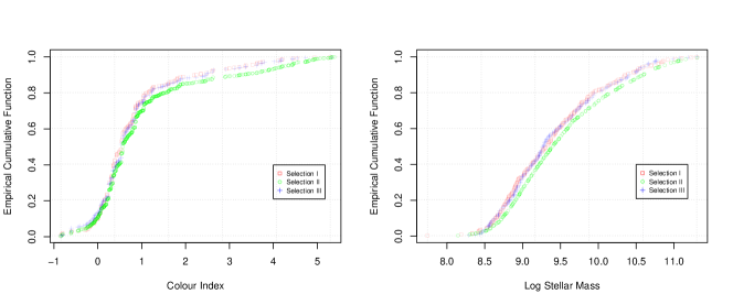
Figure 8: The empirical cumulative distribution functions for colour index (left) and stellar mass (right) for different selections by local clustering coefficient, designated by red squares, green circles and blue crosses for selections I, II and III respectively for the redshift sample $z_{2}$.

Given the different nature of distributions we should follow two-step a procedure in order to find out how colour index and stellar mass of a galaxy are determined by clustering coefficient of the galaxy: split the data set into three subsamples (or selections) according to local clustering coefficient; then compare empirical distribution functions of galaxy properties for different subsamples by two-sample tests. Thus, each redshift slice was split into three subsamples: selection I (stand-alone galaxies) $C=0$; selection II (intermediately packed galaxies) $0<C<1$; selection III (compact cliques of galaxies) $C=1$. Then distributions of different selections are tested for equality in pair-wise manner. Fig. 8 presents the empirical cumulative distribution functions of colour index and stellar mass for selections I (red squares), II (green circles) and III (blue crosses) for redshift sample $z_{2}$.
In Table 2 we present the results of the non-parametric Anderson-Darling tests. Again, here the null hypothesis states that subsamples are drawn from the same population, the alternative hypothesis states the populations are different. The $p$-value indicates the statistical significance of test, if it is less than $0.05$ the null hypothesis can be rejected with high degree of confidence. Note that the magnitude of $p$-values do not reflect the strength of the effect.
We can deduce the following conclusions from Table 2: i) the samples of selections I and III (stand-alone and densely packed in small groups of galaxies) are non-distinguishable, for all $z$-slices, with respect to both colour and stellar mass; ii) the distribution of stellar mass for selection II differs from selection I and III across all $z$-slices; iii) the distribution for colour index for selection II does not differ from selections I and III, expect when considering the $z_{2}$-slice.
The weakness of the evolutionary effects is understandable since the age differences of the nearest and farthest sample of galaxies do not exceed 400 million years. We have however to bear in mind the caution expressed already at the beginning of the paper: the database used here does not allow one to use coordinates of galaxies in 3D space with high enough precision. Indeed, the 2D slices of the real-world pictures (see Fig. 1) result from the projection of their 3D counterparts. According to Scoville et al. (2013), the binning matched to accuracy of the redshifts, thus providing optimal signal-to-noise ratio. For the density estimation the 2D projections are linearly related to a 3D volume whereas for the topological environment that might not be the case. Despite of this obvious limitation one can still retrieve information on the correlations we are interested in.

The research presented above allows one to approach probably the most important problem in cosmology, the mapping of the observable distribution of luminous matter to the underlying dark matter distribution, sometimes called the problem of biasing. The results here are derived from real-world observational data, so they are not just a description of the spatial structure, they encode information of extremely complex processes of star formation, gas and radiation transfer in different environments. So, our findings on the common behaviour in the evolution of stand-alone galaxies and cliques bring important confirmation for the Cosmic Web Detachment model (Argon-Calvo et al., 2016), identifying the events of detachment in real observations.

5 Conclusions

Here we have analysed some observed part of the Cosmic Web (COSMOS catalogue of galaxies (Ilbert et al., 2013)) by means of complex network analysis. A major distinction of our study is that we analysed galaxy samples in the same region $1^{\circ}\times 1^{\circ}$ of the celestial sphere as the previous study of Hong & Dey (2015), but for three neighbouring redshift intervals $0.88\leq z<0.91$, $0.91\leq z\leq 0.94$ and $0.94<z\leq 0.97$, marked by $z_{1}$, $z_{2}$ and $z_{3}$ accordingly.
We have developed and validated the robustness of our technique for constructing complex networks from galaxy samples using a fixed linking length method ($l=0\overset{{}^{\circ}}{.}0216$). For each redshift slice we have calculated the local complex network measures, namely degree, closeness and betweenness centralities, clustering coefficient $C(j)$ as well as the global measures, e.g. average path length $\langle\ell\rangle$, diameter $D$, average clustering coefficient $C$, number of nodes $g$ and diameter $D$ of the giant connected component GCC, mean node degree $k$, assortativity $r$.
We have not found firm evidence of evolutionary changes across complex networks, either by comparing the distributions of the local network measures or analysing global network measures. The main reason maybe due to the insufficient differences in the cosmological ages of galaxy samples.
The comparison of the computed measures of our networks with corresponding measures of random ones give us some global characteristics of the Cosmic Web in the context of complex network theory. Together these properties imply that constructed cosmic networks are not small worlds in terms of network science but rather “large worlds”.
The size of Giant Connected Component (GCC) informs about the largest cluster in a network, here it contains 63%, 64% and 78% of galaxies in $z_{1}$, $z_{2}$ and $z_{3}$ samples accordingly. The high value of assortativity coefficient $r\sim 0.80\div 0.86$ means that in the cosmic network galaxies with a similar number of links tend to be connected to one another.
Most of the local network measures have non-Gaussian distributions, often bi- or multi-modal ones (Fig. 2). The local clustering of each node $C(j)$ in the cosmic network shows a three mode distribution which allows for the discrimination between singlets and dumbbells of galaxies ($C=0$) on the one hand and cliques of galaxies ($C=1$) on the other. So, the network metrics analysed here allow for discrimination between topologically different structures.
Another goal of our study was to analyse the impact of surroundings on the astrophysical properties of galaxies, in particular colour indices and stellar masses. Doing so, besides studying the obvious impact of the immediate neighbourhood of a galaxy (which can be and is done by means of other methods too) we presented here an elaborated method to study the subtle topological features of galaxy distribution beyond its local density, as short-range clustering.
The general analysis of trends in means and standard deviations of colour indices and stellar masses across redshift slices $z_{1}$, $z_{2}$ and $z_{3}$ has not revealed substantial differences, see Table 1. Meanwhile, the comparison of distributions via non-parametric tests detects a weak evolutionary trend over the redshift span 0.88$\div$0.97 for the colour index of galaxies.
Comparison (with Anderson-Darling test) of the empirical distribution functions for astrophysical characteristics by different selections defined by the modes of clustering coefficient yields evidence of consistent and statistically significant associations between astrophysical quantities and topological selections, see Fig. 8 and Table 2.
In particular, it was shown that stand-alone galaxies with $C(j)=0$ (selection I) and galaxies densely packed in small cliques with $C(j)=1$ (selection III) are not distinguishable by colour index and stellar mass distributions.
Stellar mass distributions for galaxies with interim clustering coefficient (selection II) differ from the corresponding distributions in selections I and III. This difference holds for all redshift slices. The analogous difference in colour index distributions holds however only in the $z_{2}$ redshift slice. The latter $z_{2}$-sample has been intensively studied by other methods in the papers Scoville et al. (2013) and Hong & Dey (2015).
The presented results demonstrate the promising use of complex network theory in the study of the Cosmic Web. With the improving accuracy of redshift values for galaxies, we hope that in future, this will allow the cosmic network to be studied in 3D which will in turn provide more accurate results.

References

- Albert & Barabási (2002) Albert R., Barabási A. L., 2002, Rev. Mod. Phys., 74, 47
- Anderson & Darling (1954) Anderson T. W., Darling D. A., 1954, J. Amer. Stist. Assoc., 29, 765.
- Ankerst et al. (1999) Ankerst M., Breunig M., Kriegel H.-P., Sander J., 1999, Proc. ACM SIGMOD‘99 Int. Conf. on Management of Data, Philadelphia PA, 49.
- Argon-Calvo et al. (2016) Aragon-Calvo M. A., Neyrinck M. C., Silk J., 2016, arXiv:1607.07881
- Bardeen et al. (1986) Bardeen J. M., Bond J. R., Kaiser N., Szalay A. S., 1986, Astrophys. J., 304, 15.
- Barrat et al. (2008) Barrat A., Barthelemy M., Vespignani A., 2008, Cambridge: Cambridge University Press
- Bond et al. (1996) Bond J. R., Kofman L., Pogosyan D., 1996, Nature, 380, 603.
- Brandes (2001) Brandes U.A., 2011,Journal of mathematical sociology, 25(2), 163-77
- Brouwer et al. (2016) Brouwer M.M., Cacciato M., Dvornik A. et al., 2016, MNRAS, 462, 4451
- Cautun et al. (2014) Cautun M., van de Weygaert R., Jones B. J. T., Frenk C. S., 2014, MNRAS, 441, 2923.
- Chen et al. (2015) Chen Y.-C., Ho S., Freeman P. E., Genovese C. R., Wasserman L., 2015, MNRAS, 454, 1140.
- Chen et al. (2016) Chen Y.-C., Ho S., Brinkmann J., Freeman P. E., Genovese C. R., Schneider D. P., Wasserman L., 2016, MNRAS, 461, 3896.
- Coutinho et al. (2016) Coutinho B., Hong S., Albrecht K., Dey A., Baraba’si A.-L., Torrey P., Vogelsberger M., Hernquist L., 2016, arXiv:1604.03236.
- Dorogovtsev & Mendes (2003) Dorogovtsev S. N., Mendes J. F. F., 2003, Oxford: Oxford University Press
- Ester et al. (1997) Ester M., Kriegel H.-P., Sander J., and Xu X., 1996, Proceedings of the Second International Conference on Knowledge Discovery and Data Mining (KDD-96). AAAI Press. pp. 226-231.
- Erdos & Rényi (1960) Erdös P., & Rényi A., 1960, Pub. Math. Inst. Hung. Acad. Sci., 5, 17.
- Fronczak et al. (2004) Fronczak, A. Fronczak, P. Holyst, J. Phys. Rev., E 70, 2004.
- Hahn (2014) Hahn O., 2014, arXiv:1412.5197
- Hartigan & Hartigan (1985) Hartigan J.A., Hartigan P.M., 1985, Ann. Statist., 13, 70.
- Hong et al. (2016) Hong S., Coutinho B., Dey A., Barabasi A.-L., Vogelsberger M., Hernquist L., Gebhardt K., 2016, arXiv:1603.02285.
- Hong & Dey (2015) Hong S. & Dey A. 2015, MNRAS, 450, 1999.
- Ilbert et al. (2013) Ilbert O., McCracken H. J., Le Févre O., Capak P., Dunlop J. et al., 2013, Astron. & Astrophys., 556, 55.
- Kolmogorov (1933) Kolmogorov A., 1933, G. Ist. Ital. Attuari., 4, 83.
- Kuutma, Tamm & Tempel (2017) Kuutma T., Tamm A., Tempel E., 2017, Astron. & Astrophys., 600, L6
- Leclercq et al. (2016) Leclercq F., Lavaux G., Jasche J., Wandelt B., 2016, JCAP, 8, 027.
- Lee & Yepes (2016) Lee J. & Yepes G., 2016, arXiv:1608.01422
- Libeskind et al. (2017) Libeskind N.I., van de Weygaert R., Cautun M. et al., 2017, arXiv:1705.03021
- Mann & Whitney (1947) Mann H.B., Whitney D. R., 1947, Annals of Mathematical Statistics, 18, 50.
- McCracken et al (2012) McCracken H. J., Milvang-Jensen B., Dunlop J., Franx M. et al., 2012, Astron. & Astrophys., Volume 544, id.A156, 11 pp.
- Newman (2010) Newman M., 2010, Oxford: Oxford University Press
- Pace et al. (2015) Pace F., Manera M., Bacon D. J., Crittenden R., Percival W. J., 2015, MNRAS, 454, 708.
- Pranav et al. (2016) Pranav P., Edelsbrunner H., van de Weygaert R., Vegter G., Kerber M., Jones B. J. T., Wintraecken M., 2016, arXiv:1608.04519.
- Press & Davis (1982) Press W.H., Davis M., 1982, Astrophys. J., 259, 249.
- Ramachandra & Shandarin (2016) Ramachandra N. S. & Shandarin, S. F., 2016, arXiv:1608.05469.
- Scoville et al. (2013) Scoville N., et al., 2013, ApJS, 206, 3.
- Smirnov (1948) Smirnov N., 1948, Ann. Math. Statist., 19, 279.
- Watts and Strogatz (1998) Watts D.J., Strogatz S.H., 1998, nature, 393(6684), 440-2.
- Weisstein (2002) Weisstein E., 2002, Wolfram Research, Inc.
- Wilcoxon (1945) Wilcoxon F., 1945, Biometrics Bulletin, 1, 80.
- Zhao et al. (2015) Zhao C., Kitaura F.-S., Chuang C.-H., Prada F., Yepes G., Tao C., 2015, MNRAS, 451, 4266.
- (41)