Empirical optimal transport on countable metric spaces: Distributional limits and statistical applications

Abstract

We derive distributional limits for empirical transport distances between probability measures supported on countable sets. Our approach is based on sensitivity analysis of optimal values of infinite dimensional mathematical programs and a delta method for non-linear derivatives. A careful calibration of the norm on the space of probability measures is needed in order to combine differentiability and weak convergence of the underlying empirical process. Based on this we provide a sufficient and necessary condition for the underlying distribution on the countable metric space for such a distributional limit to hold. We give an explicit form of the limiting distribution for ultra-metric spaces.
Finally, we apply our findings to optimal transport based inference in large scale problems. An application to nanoscale microscopy is given.

MSC subject classification Primary 60F05, 60B12, 62E20; Secondary 90C08, 90C31, 62G10

Keywords optimal transport, Wasserstein distance, empirical process, limit law, statistical testing

1 Introduction

Optimal transport based distances between probability measures (see e.g., Rachev and Rüschendorf, (1998) or Villani, (2008) for a comprehensive treatment), e.g., the Wasserstein distance (Vasershtein,, 1969), which is also known as Earth Movers distance (Rubner et al.,, 2000), Kantorovich-Rubinstein distance (Kantorovich and Rubinstein,, 1958) or Mallows distance (Mallows,, 1972), are of fundamental interest in probability and statistics, with respect to both theory and practice. The $p$-th Wasserstein distance (WD) between two probability measures $\mu$ and $\nu$ on a Polish metric space $(\mathcal{X},d)$ is given by

$$W_{p}(\mu,\nu)=\left(\inf_{\pi}\int_{\mathcal{X}\times\mathcal{X}}d(x,y)^{p}d\pi(x,y)\right)^{1/p}$$ (1)

for $p\in[1,\infty)$, the infimum is taken over all probability measures $\pi$ on the product space $\mathcal{X}\times\mathcal{X}$ with marginals $\mu$ and $\nu$.
The WD metrizes weak convergence of a sequence of probability measures on $(\mathcal{X},d)$ together with convergence of its first $p$ moments and has become a standard tool in probability, e.g., to study limit laws (e.g., Johnson and Samworth, (2005); Rachev and Rüschendorf, (1994); Shorack and Wellner, (1986)), to derive bounds for Monte Carlo computation schemes such as MCMC (e.g., Eberle, (2014); Rudolf and Schweizer, (2015)), for point process approximations (Barbour and Brown,, 1992; Schuhmacher,, 2009), bootstrap convergence (Bickel and Freedman,, 1981) or to quantify measures of risk (Rachev et al.,, 2011). Besides of its theoretical importance, the WD is used in many applications as an empirical measure to compare complex objects, e.g., in image retrieval (Rubner et al.,, 2000), deformation analysis (Panaretos and Zemel,, 2016), meta genomics (Evans and Matsen,, 2012), computer vision (Ni et al.,, 2009), goodness-of-fit testing (Munk and Czado,, 1998; del Barrio et al.,, 2000) and machine learning (Rolet et al.,, 2016).

In such applications the WD has to be estimated from a finite sample of the underlying measures. This raises the question how fast the empirical Wasserstein distance (EWD), i.e., when either $\mu$ or $\nu$ (or both) are estimated by the empirical measures $\boldmath{\hat{\mu}_{n}}=\frac{1}{n}\sum_{i=1}^{n}\delta_{X_{i}}$ (and $\boldmath{\hat{\nu}_{m}}=\frac{1}{m}\sum_{i=1}^{m}\delta_{Y_{i}}$) approaches WD. Ajtai et al., (1984) investigated the rate of convergence of EWD for the uniform measure on the unit square, Talagrand, (1992) and Talagrand, (1994) extended this to higher dimensions. Horowitz and Karandikar, (1994) then provided non-asymptotic bounds for the average speed of convergence for the empirical 2-Wasserstein distance. There are several refinements of these results, e.g., Boissard and Gouic, (2014), Fournier and Guillin, (2014) and Weed and Bach, (2017).

As a natural extension of such results, there is a long standing interest in distributional limits for EWD, in particular motivated from statistical applications. Most of this work is restricted to the univariate case $\mathcal{X}\subset\mathbb{R}$. Munk and Czado, (1998) derived central limit theorems for a trimmed WD on the real line when $\mu\neq\nu$ whereas del Barrio et al., 1999a ; del Barrio et al., 1999b consider the empirical Wasserstein distance when $\mu$ belongs to a parametric family of distributions for the assessment of goodness of fit, e.g., for a Gaussian location scale family. In a similar spirit del Barrio et al., (2005) provided asymptotics for a weighted version of the empirical 2-Wasserstein distance in one dimension and Freitag and Munk, (2005) derive limit laws for semiparametric models, still restricted to the univariate case. There are also several results for dependent data in one dimension, e.g., Dede, (2009), Dedecker and Merlevede, (2015). For a recent survey we refer to Bobkov and Ledoux, (2014) and Mason, (2016) and references therein. A major reason of the limitation to dimension $D=1$ is that only for $\mathcal{X}\subset\mathbb{R}$ (or more generally a totally ordered space) the coupling which solves (1) is known explicitly and can be expressed in terms of the quantile functions $F^{-1}$ and $G^{-1}$ of $\mu$ and $\nu$, respectively, as $\pi=(F^{-1}\times G^{-1})\#\mathcal{L}$, where $\mathcal{L}$ is the Lebesgue measure on $[0,1]$ (see Mallows, (1972)). All the above mentioned work relies essentially on this fact. For higher dimensions only in specific settings such a coupling can be computed explicitly and then can be used to derive limit laws (Rippl et al.,, 2016). Already for $D=2$ Ajtai et al., (1984) indicate that the scaling rate for the limiting distribution of $W_{1}(\hat{\mu}_{n},\mu)$ when $\mu$ is the uniform measure on $\mathcal{X}=[0,1]^{2}$ (if it exists) must be of complicated nature as it is bounded from above and below by a rate of order $\sqrt{n\log(n)}$.

Recently, del Barrio and Loubes, (2017) gave distributional limits for the quadratic EWD in general dimension with a scaling rate $\sqrt{n}$. This yields a (non-degenerate) normal limit in the case $\mu\neq\nu$, i.e., when the data generating measure is different from the measure to be compared with (extending Munk and Czado, (1998) to $D>1$). Their result centers the EWD with an expected EWD (whose value is typically unknown) instead of the true WD and requires $\mu$ and $\nu$ to have a positive Lebesgue density on the interior of their convex support. Their proof uses the uniqueness and stability of the optimal transportation potential (i.e., the minimizer of the dual transportation problem, see Villani, (2003) for a definition and further results) and the Efron-Stein variance inequality. However, in the case $\mu=\nu$, their distributional limit degenerates to a point mass at $0$, underlining the fundamental difficulty of this problem again.

An alternative approach has been advocated recently in Sommerfeld and Munk, (2018) who restrict to finite spaces $\mathcal{X}=\left\{x_{1},\ldots,x_{N}\right\}$. They derive limit laws for the EWD for $\mu=\nu$ (and $\mu\neq\nu$), which requires a different scaling rate. In this paper we extend their work to measures $\bm{r}=(r_{x})_{x\in\mathcal{X}}$ that are supported on countable metric spaces $(\mathcal{X},d)$. Our approach links the asymptotic distribution of the EWD on the one hand to the issue of weak convergence of the underlying multinomial process associated with $\hat{\mu}_{n}$ with respect to a weighted $\ell^{1}$-norm (for fixed, but arbitrary $x_{0}\in\mathcal{X}$)

$$\|\bm{r}\|_{\ell^{1}(d^{p})}=\sum_{x\in\mathcal{X}}d^{p}(x,x_{0})\left|r_{x}\right|+\left|r_{x_{0}}\right|,$$ (2)

and on the other hand to infinite dimensional sensitivity analysis of the underlying linear program. Notably, we obtain a necessary and sufficient condition for such a limit law, which sheds some light on the limitation to approximate the WD between continuous measures for $D\geq 2$ by discrete random variables.

The outline of this paper is a follows. In Section 2 we give distributional limits for the EWD of measures that are supported on a countable metric space. In short, this limit can be characterized as the optimal value of an infinite dimensional linear program applied to a Gaussian process over the set of dual solutions. The main ingredients of the proof are the directional Hadamard differentiability of the Wasserstein distance on countable metric spaces and the delta method for non-linear derivatives. We want to emphasize that the delta method for non-linear derivatives is not a standard tool (see Shapiro, (1991); Römisch, (2004)). Moreover, for the delta method to work here weak convergence in the weighted $\ell^{1}$-norm (2) of the underlying empirical process $\sqrt{n}(\hat{\mathbf{r}}_{n}-\bm{r})$ is required as the directional Hadamard differentiability is proven w.r.t. this norm. We cannot prove the directional Hadamard differentiability with our methods w.r.t. the $\ell^{1}$-norm as the space of probability measures with finite $p$-th moment is not complete with respect to the $\ell^{1}$-norm, see Section 2.5 for more details. We find that

$$\sum_{x\in\mathcal{X}}d^{p}(x,x_{0})\sqrt{r_{x}}<\infty$$ (3)

is necessary and sufficient for weak convergence. This condition arises from Jain’s CLT (Jain,, 1977). Furthermore, we examine (3) in a more detailed way in Section 2.3. We give examples and counterexamples for (3) and discuss whether the condition holds in case of an approximation of continuous measures. Further, we examine under which assumptions it follows that (3) holds for all $p^{\prime}\leq p$ if it is fulfilled for $p$, and put it in relation to its one-dimensional counterpart, see del Barrio et al., 1999b . We close this section by discussing simplifications for ground spaces $\mathcal{X}$ with bounded diameter.
In Section 3 we specify the case where the metric structure on the ground space is given by a rooted tree with weighted edges. In this case we can provide a simplified limiting distribution and use its explicit formula to derive a distributional upper bound for general metric spaces.
In Section 4 we combine this with a well known lower bound (Pele and Werman,, 2009) to derive a computationally efficient strategy to test for the equality of two measures $\bm{r}$ and $\bm{s}$ on a countable metric space. Furthermore, we derive an explicit formula of the upper bound from Section 3 in the case of the support of $\bm{r}$ being a regular grid.
An application of our results to data from single marker switching microscopy imaging is given in Section 5. As the number of pixels typically is of magnitude $10^{5}$ - $10^{6}$ this challenges the assumptions of a finite space underlying the limit law in Sommerfeld and Munk, (2018) and our work provides the theoretical justification to perform EWD based inference in such a case. Finally, we stress that our results can be extended to many other situations, e.g., the comparison of $k$ samples and when the underlying data are dependent, as soon as a weak limit of the underlying empirical process w.r.t. the weighted $\ell^{1}$-norm (2) can be shown.

2 Distributional Limits

2.1 Wasserstein distance on countable metric spaces

Let throughout the following $\mathcal{X}=\left\{x_{1},x_{2},\ldots\right\}$ be a countable metric space equipped with a metric $d\colon\mathcal{X}\times\mathcal{X}\to\mathbb{R}_{+}$. The probability measures on $\mathcal{X}$ are infinite dimensional vectors $\bm{r}$ in

$$\mathcal{P}(\mathcal{X})=\left\{\bm{r}=(r_{x})_{x\in\mathcal{X}}:r_{x}\geq 0\quad\forall x\in\mathcal{X}\text{ and }\sum_{x\in\mathcal{X}}r_{x}=1\right\}.$$

We want to emphasize that we consider the discrete topology on $\mathcal{X}$ and do not embed $\mathcal{X}$ for example in $\mathbb{R}^{d}$. This implies that the support of any probability measure $\bm{r}\in\mathcal{P}(\mathcal{X})$ is the union of points $x\in\mathcal{X}$ such that $r_{x}>0$. The $p$-th Wasserstein distance ($p\geq 1$) then becomes

$$W_{p}(\bm{r},\bm{s})=\left\{\min_{\bm{w}\in\Pi(\bm{r},\bm{s})}\sum_{x,x^{\prime}\in\mathcal{X}}d^{p}(x,x^{\prime})w_{x,x^{\prime}}\right\}^{1/p},$$ (4)

where

$$\Pi(\bm{r},\bm{s})=\Big{\{}\bm{w}\in\mathcal{P}(\mathcal{X}\times\mathcal{X}):\sum_{x^{\prime}\in\mathcal{X}}w_{x,x^{\prime}}=r_{x}\\ \text{ and }\sum_{x\in\mathcal{X}}w_{x,x^{\prime}}=s_{x^{\prime}}\quad\forall x,x^{\prime}\in\mathcal{X}\Big{\}}$$

is the set of all couplings between $\bm{r}$ and $\bm{s}$. Furthermore, let

$$\mathcal{P}_{p}(\mathcal{X})=\left\{\bm{r}\in\mathcal{P}(\mathcal{X}):\sum_{x\in\mathcal{X}}d^{p}(x,x_{0})r_{x}<\infty\right\}$$

be the set of probability measures on the countable metric space $\mathcal{X}$ with finite $p$-th moment w.r.t. $d$. Here, $x_{0}\in\mathcal{X}$ is arbitrary and we want to mention that the space is independent of the choice of $x_{0}$. We need to introduce the weighted $\ell^{1}$-space $\ell^{1}_{d^{p}}(\mathcal{X})$ which is defined via the weighted $\ell^{1}$-norm (2) as in this case the set of probability measures with finite $p$-th moment is a closed subset and hence complete itself. This will play a crucial role in the proof of the directional Hadamard differentiability (see Appendix A.1). The weighted $\ell^{1}$-norm (2) can be extended in the following way to sequences on $\mathcal{X}\times\mathcal{X}$ and hence to $\mathcal{P}_{p}(\mathcal{X}\times\mathcal{X})$

$$\|\bm{w}\|_{\ell^{1}(d^{p})}=\sum_{x,x^{\prime}\in\mathcal{X}}d^{p}(x_{0},x)\left|w_{x,x^{\prime}}\right|+\left|w_{x_{0},x^{\prime}}\right|\\ +\sum_{x,x^{\prime}\in\mathcal{X}}d^{p}(x_{0},x^{\prime})\left|w_{x,x^{\prime}}\right|+\left|w_{x,x_{0}}\right|.$$

2.2 Main Results

Before we can state the main results we need a few definitions.
Define the empirical measure generated by i.i.d. random variables $X_{1},\ldots,X_{n}$ from the measure $\bm{r}$ as

$$\hat{\mathbf{r}}_{n}=(\hat{r}_{n,x})_{x\in\mathcal{X}},\text{ where }\hat{r}_{n,x}=\frac{1}{n}\sum_{k=1}^{n}\mathds{1}_{\left\{X_{k}=x\right\}},$$ (5)

and $\hat{\mathbf{s}}_{m}$ is defined in the same way by $Y_{1},\ldots,Y_{m}\overset{i.i.d.}{\sim}\bm{s}$. In the following we will denote weak convergence by $\xrightarrow{\mathscr{D}}$ and furthermore, let

$$\ell^{\infty}(\mathcal{X})=\left\{(a_{x})_{x\in\mathcal{X}}\in\mathbb{R}^{\mathcal{X}}:\sup_{x\in\mathcal{X}}\left|a_{x}\right|<\infty\right\}$$

and

$$\ell^{1}(\mathcal{X})=\left\{(a_{x})_{x\in\mathcal{X}}\in\mathbb{R}^{\mathcal{X}}:\sum_{x\in\mathcal{X}}\left|a_{x}\right|<\infty\right\}.$$

Finally, we also require a weighted version of the $\ell^{\infty}$-norm to characterize the set of dual solutions:

$$\|a\|_{\ell^{\infty}(1/d^{p})}=\max\left(\left|a_{x_{0}}\right|,\sup_{x\neq x_{0}\in\mathcal{X}}\left|d^{-p}(x,x_{0})a_{x}\right|\right),$$

for $p\geq 1$. The space $\ell^{\infty}_{d^{-p}}(\mathcal{X})$ contains all elements which have a finite $\|\cdot\|_{\ell^{\infty}(1/d^{p})}$-norm.
For $\bm{r},\bm{s}\in\mathcal{P}_{p}(\mathcal{X})$ we define the following convex sets

$$\mathcal{S}^{*}(\bm{r},\bm{s})=\Big{\{}(\bm{\lambda},\bm{\mu})\in\ell^{\infty}_{d^{-p}}(\mathcal{X})\times\ell^{\infty}_{d^{-p}}(\mathcal{X}):\left\langle\bm{r},\bm{\lambda}\right\rangle+\left\langle\bm{s},\bm{\mu}\right\rangle=W_{p}^{p}(\bm{r},\bm{s})$$ (6)

$$\lambda_{x}+\mu_{x^{\prime}}\leq d^{p}(x,x^{\prime})\quad\forall x,x^{\prime}\in\mathcal{X}\Big{\}}$$

and

$$\mathcal{S}^{*}(\bm{r})=\Big{\{}\bm{\lambda}\in\ell^{\infty}_{d^{-p}}(\mathcal{X}):\lambda_{x}-\lambda_{x^{\prime}} \leq d^{p}(x,x^{\prime})\quad\forall x,x^{\prime}\in\mathrm{supp}(\bm{r})\Big{\}},$$ (7)

with $\mathrm{supp}(\bm{r})=\left\{x\in\mathcal{X}\colon r_{x}>0\right\}$. For our limiting distributions we define the following (multinomial) covariance structure

$$\Sigma(\bm{r})=\begin{cases}r_{x}(1-r_{x})&\text{ if }x=x^{\prime},\\ -r_{x}r_{x^{\prime}}&\text{ if }x\neq x^{\prime}.\end{cases}$$ (8)

Theorem 2.1.

Let $(\mathcal{X},d)$ be a countable metric space and $\bm{r},\bm{s}\in\mathcal{P}_{p}(\mathcal{X})$, $p\geq 1$, and $\hat{\mathbf{r}}_{n}$ be generated by i.i.d. samples $X_{1},...,X_{n}\sim\bm{r}$. Furthermore, let $\mathbf{G}\sim\mathcal{N}(0,\Sigma(\bm{r}))$ be a Gaussian process with $\Sigma$ as defined in (8). Assume (3) for some $x_{0}\in\mathcal{X}$. Then

1. $$n^{\frac{1}{2p}}W_{p}(\hat{\mathbf{r}}_{n},\bm{r})\xrightarrow{\mathscr{D}}\left\{\max_{\bm{\lambda}\in\mathcal{S}^{*}(\bm{r})}\langle\mathbf{G},\bm{\lambda}\rangle\right\}^{\tfrac{1}{p}},\text{ as }n\to\infty.$$ (9)

2. In the case where $\bm{r}\neq\bm{s}$ it holds for $n\to\infty$

   $$n^{\frac{1}{2}}(W_{p}(\hat{\mathbf{r}}_{n},\bm{s})-W_{p}(\bm{r},\bm{s}))\xrightarrow{\mathscr{D}}\\ \frac{1}{p}W_{p}^{1-p}(\bm{r},\bm{s})\left\{\max_{(\bm{\lambda},\bm{\mu})\in\mathcal{S}^{*}(\bm{r},\bm{s})}\langle\mathbf{G},\bm{\lambda}\rangle\right\}.$$ (10)

Note, that we obtain different scaling rates under equality of measures $\bm{r}=\bm{s}$ (null-hypothesis) and the case $\bm{r}\neq\bm{s}$ (alternative), which has important statistical consequences. For $\bm{r}\neq\bm{s}$ we are in the regime of the standard C.L.T. rate $\sqrt{n}$, but for $\bm{r}=\bm{s}$ we get the rate $n^{\frac{1}{2p}}$, which is strictly slower for $p>1$.

Remark 2.2 (Degeneracy of limit law).

We would like to discuss in which settings the limit distribution in (9) is degenerate.
In the case that $\bm{r}$ has full support the limit degenerates to a point mass at $0$ if $\mathcal{S}^{*}(\bm{r})$ contains only constant elements, i.e., for a $c\in\mathbb{R}$ $\lambda_{x}=c$ for all $x\in\mathcal{X}$. Then, the right hand side in (9) becomes zero. $\mathcal{S}^{*}(\bm{r})$ contains only constant elements if and only if the space $\mathcal{X}$ has no isolated point.
Specifying $\mathcal{X}$ to be a subset of the real line $\mathbb{R}$ that has no isolated point it follows from Theorem 7.11. in Bobkov and Ledoux, (2014) that scaling with $\sqrt{n}$ provides then a non-degenerate limit law. On the other hand, as soon as $\mathcal{X}\subset\mathbb{R}$ contains an isolated point our rate coincides with the rate given in Bobkov and Ledoux, (2014).

Remark 2.3.

1. Note, that in Theorem b) b) where the measures are not the same the objective function in (10) is independent of the second component $\bm{\mu}$ of the feasible set $\mathcal{S}^{*}(\bm{r},\bm{s})$. This is due to the fact that in $W_{p}(\hat{\mathbf{r}}_{n},\bm{s})$ the second component is not random.

2. Observe, that the limit in (10) is normally distributed if the set $\mathcal{S}^{*}(\bm{r},\bm{s})$ is a singleton up to a constant shift. In the case of finite $\mathcal{X}$ conditions for $\mathcal{S}^{*}(\bm{r},\bm{s})$ to be a singleton up to a constant shift are known (Hung et al.,, 1986; Klee and Witzgall,, 1968).

3. Parallel to our work del Barrio and Loubes, (2017) showed asymptotic normality of the quadratic EWD in general dimensions for the case $\bm{r}\neq\bm{s}$. Their results require the measures to have moments of order $4+\delta$ for some $\delta>0$ and positive density on their convex support. Their proof relies on a Stein-identity. In the case $\bm{r}=\bm{s}$ the limiting distribution is degenerated, in contrast to Thm. 2.1 a).

4. The limiting distribution in the case $\bm{r}=\bm{s}$ can also be written as

   $$\left\{\max_{\bm{\lambda}\in\mathcal{S}^{*}(\bm{r})}\langle\mathbf{G},\bm{\lambda}\rangle\right\}^{\tfrac{1}{p}}=\left\{\inf_{\bm{z}(\bm{r})\in\ell^{\infty}_{d^{-p}}(\mathcal{X})}W_{p}(\mathbf{G}^{+}+\bm{z}(\bm{r}),\mathbf{G}^{-}+\bm{z}(\bm{z}))\right\}^{1/p},$$

   where $\mathbf{G}^{+}$ and $\mathbf{G}^{-}$ denotes the (pathwise) decomposition of the Gaussian process $\mathbf{G}$, such that $\mathbf{G}=\mathbf{G}^{+}-\mathbf{G}^{-}$ and $\bm{z}(\bm{r})$ is related to $\bm{r}$ in the sense that $z_{x}=0$ for that $x\in\mathcal{X}$ such that $r_{x}=0$. Further, we would like to emphasize that the set of dual solutions $\mathcal{S}^{*}(\bm{r})$ is independent of $\bm{r}$, if the support of $\bm{r}$ is full, i.e.,

   $$\mathcal{S}^{*}=\Big{\{}\bm{\lambda}\in\ell^{\infty}_{d^{-p}}(\mathcal{X}):\lambda_{x}-\lambda_{x^{\prime}}\leq d^{p}(x,x^{\prime})\quad\forall x,x^{\prime}\in\mathcal{X}\Big{\}}.$$ (11)

   This offers a universal strategy to simulate the limiting distribution on trees independent of $\bm{r}$. For more details see Appendix A.2.

For statistical applications it is also interesting to consider the two sample case, extensions to $k$-samples, $k\geq 2$ being obvious then.

Theorem 2.4.

Under the same assumptions as in Thm. 2.1 and with $\hat{\mathbf{s}}_{m}$ generated by $Y_{1},\ldots,Y_{m}\overset{iid}{\sim}\bm{s}$, independently of $X_{1},\ldots,X_{n}$ and $\mathbf{H}\sim\mathcal{N}(0,\Sigma(\bm{s}))$, which is independent of $\mathbf{G}$, and the extra assumption that $\bm{s}$ also fulfills (3) the following holds.

1. Let $\rho_{n,m}=(nm/(n+m))^{1/2}$. If $\bm{r}=\bm{s}$ and $\min(n,m)\to\infty$ such that $m/(n+m)\to\alpha\in[0,1]$ we have

   $$\rho^{1/p}_{n,m}W_{p}(\hat{\mathbf{r}}_{n},\hat{\mathbf{s}}_{m})\xrightarrow{\mathscr{D}}\left\{\max_{\bm{\lambda}\in\mathcal{S}^{*}(\bm{r})}\langle\mathbf{G},\bm{\lambda}\rangle\right\}^{\tfrac{1}{p}}.$$ (12)

2. For $\bm{r}\neq\bm{s}$ and $n,m\to\infty$ such that $\min(n,m)\to\infty$ and $m/(n+m)\to\alpha\in[0,1]$ we have

   $$\rho_{n,m} (W_{p}(\hat{\mathbf{r}}_{n},\hat{\mathbf{s}}_{m})-W_{p}(\bm{r},\bm{s}))\xrightarrow{\mathscr{D}}$$ (13)

   $$\frac{1}{p}W_{p}^{1-p}(\bm{r},\bm{s})\left\{\max_{(\bm{\lambda},\bm{\mu})\in\mathcal{S}^{*}(\bm{r},\bm{s})}\sqrt{\alpha}\langle\mathbf{G},\bm{\lambda}\rangle+\sqrt{1-\alpha}\left\langle\mathbf{H},\bm{\mu}\right\rangle\right\}.$$

Remark 2.5.

In the case of dependent data analogous results to Thm. 2.1 and 2.4 will hold, as soon as the weak convergence of the empirical process w.r.t. the $\|\cdot\|_{\ell^{1}(d^{p})}$-norm is valid. All other steps of the proof remain unchanged.

The rest of this subsection is devoted to the proofs of Theorem 2.1 and Theorem 2.4.

Proof of Thm. 2.1 and Thm. 2.4.

To prove these two theorems we use the delta method A.2. Therefore, we need to verify (1.) directional Hadamard differentiability of $W_{p}(\cdot,\cdot)$ and (2.) weak convergence of $\sqrt{n}(\hat{\mathbf{r}}_{n}-\bm{r})$. We mention that the delta method required here is not standard as the directional Hadamard derivative is not linear (see Römisch, (2004), Shapiro, (1991) or Dümbgen, (1993)).

1. In Appendix A.1, Theorem A.3 directional Hadamard differentiability of $W_{p}$ is shown with respect to the $\|\cdot\|_{\ell^{1}(d^{p})}$-norm (2).
   

2. The weak convergence of the empirical process w.r.t. the $\|\cdot\|_{\ell^{1}(d^{p})}$-norm is addressed in the following lemma.

   Lemma 2.6.

   Let $X_{1},\ldots,X_{n}\sim\bm{r}$ be i.i.d. taking values in a countable metric space $(\mathcal{X},d)$ and let $\hat{\mathbf{r}}_{n}$ be the empirical measure as defined in (5). Then

   $$\sqrt{n}(\hat{\mathbf{r}}_{n}-\bm{r})\xrightarrow{\mathscr{D}}\mathbf{G}$$

   with respect to the $\|\cdot\|_{\ell^{1}(d^{p})}$-norm, where $\mathbf{G}$ is a Gaussian process with mean 0 and covariance structure

   $$\Sigma(\bm{r})=\begin{cases}r_{x}(1-r_{x})&\text{ if }x=x^{\prime},\\ -r_{x}r_{x^{\prime}}&\text{ if }x\neq x^{\prime},\end{cases}$$

   as given in (8) if and only if condition (3) is fulfilled.

   Proof of Lemma.

   The weighted $\ell^{1}$-space $\ell^{1}_{d^{p}}$ is according to Prop. 3, Maurey, (1973) of cotype 2, hence $\sqrt{n}(\hat{\mathbf{r}}_{n}-\bm{r})$ converges weakly w.r.t. the $\ell^{1}(d^{p})$-norm by Corollary 1 in Jain, (1977) if and only if the summability condition (3) is fulfilled. ∎

Theorem a) a) is now a straight forward application of the delta method A.2 and the continuous mapping theorem for $f(x)=x^{1/p}$.

For Theorem b) b) we use again the delta method, but this time in combination with the chain rule for directional Hadamard differentiability (Prop. 3.6 (i), Shapiro, (1990)).

The proof of Theorem 2.4 works analogously. Note, that under the assumptions of the theorem it holds $(\bm{r}=\bm{s})$

$$\rho_{n,m}((\hat{\mathbf{r}}_{n},\hat{\mathbf{s}}_{m})-(\bm{r},\bm{s}))\\ =\left(\sqrt{\frac{m}{n+m}}\sqrt{n}(\hat{\mathbf{r}}_{n}-\bm{r}),\sqrt{\frac{n}{n+m}}\sqrt{m}(\hat{\mathbf{s}}_{m}-\bm{s})\right)\\ \xrightarrow{\mathscr{D}}(\sqrt{\alpha}\mathbf{G},\sqrt{1-\alpha}\mathbf{G}^{\prime})$$ (14)

with $\mathbf{G}^{\prime}\overset{\mathcal{D}}{=}\mathbf{G}$. For further explanations see Appendix A.2. ∎

2.3 Examination of the summability condition (3)

According to Lemma 2.6 condition (3) is necessary and sufficient for the weak convergence with respect to the $\|\cdot\|_{\ell^{1}(d^{p})}$-norm defined in (2). As this condition is crucial for our main theorem and we are not aware of a comprehensive discussion, we will provide such in this section.

The following question arises. ”If the condition holds for $p$ does it then also hold for all $p^{\prime}\leq p$?” This is not true in general, but it is true if $\mathcal{X}$ has no accumulation point (i.e., is discrete in the topological sense).

Lemma 2.7.

Let $\mathcal{X}$ be a space without any accumulation point with respect to the metric $d$. If condition (3) holds for $p$, then it also holds for all $1\leq p^{\prime}\leq p$.

Proof.

Let $\mathcal{X}$ be a space without an accumulation point, i.e., there exists $\epsilon>0$ such that $d(x,x^{\prime})>\epsilon$ for all $x\neq x^{\prime}\in\mathcal{X}$. Then,

$$\sum_{x\in\mathcal{X}}d^{p}(x_{0},x)\sqrt{r_{x}} =\epsilon^{p}\sum_{x\in\mathcal{X}}\left(\frac{d(x_{0},x)}{\epsilon}\right)^{p}\sqrt{r_{x}}$$

$$\geq\epsilon^{p}\sum_{x\in\mathcal{X}}\left(\frac{d(x_{0},x)}{\epsilon}\right)^{p^{\prime}}\sqrt{r_{x}}$$

$$=\epsilon^{p/{p^{\prime}}}\sum_{x\in\mathcal{X}}d^{p^{\prime}}(x_{0},x)\sqrt{r_{x}}.$$

∎

Exponential families

As we will see, condition (3) is fulfilled for many well known distributions including the Poisson distribution, geometric distribution or negative binomial distribution with the euclidean distance as the ground measure $d$ on $\mathcal{X}=\mathbb{N}$.

Theorem 2.8.

Let $(\mathcal{P}_{\bm{\eta}})_{\bm{\eta}}$ be an s-dimensional standard exponential family (SEF) (see Lehmann and Casella, (1998), Sec. 1.5) of the form

$$r_{x}^{\bm{\eta}}=h_{x}\exp\left(\sum_{i=1}^{s}\eta_{i}T_{x}^{i}-A(\bm{\eta})\right).$$ (15)

The summability condition (3) is fulfilled if $(\mathcal{P}_{\bm{\eta}})_{\bm{\eta}}$ satisfies

• $h_{x}\geq 1$ for all $x\in\mathcal{X}$,

• the natural parameter space $\mathcal{N}$ is closed with respect to multiplication with $\frac{1}{2}$, i.e., $\sum_{x\in\mathcal{X}}r^{\bm{\eta}}_{x}<\infty\Rightarrow\sum_{x\in\mathcal{X}}r^{\bm{\eta}/2}_{x}<\infty$,

• the $p$-th moment w.r.t. the metric $d$ on $\mathcal{X}$ exists, i.e., $\sum_{x\in\mathcal{X}}d^{p}(x,x_{0})r^{\bm{\eta}}_{x}<\infty$ for some arbitrary, but fixed $x_{0}\in\mathcal{X}$.

Proof.

For the SEF in (15) condition (3) reads

$$\sum_{x\in\mathcal{X}}d^{p}(x_{0},x) \sqrt{\exp\left(\sum_{i=1}^{s}\eta_{i}T^{i}_{x}-A(\bm{\eta})\right)h_{x}}$$

$$=\frac{1}{\sqrt{\lambda(\bm{\eta})}}\sum_{x\in\mathcal{X}}d^{p}(x_{0},x)\exp\left(\tfrac{1}{2}\sum_{i=1}^{s}\eta_{i}T_{x}^{i}\right)\sqrt{h_{x}}$$ (16)

$$\leq\frac{\lambda(\tfrac{1}{2}\bm{\eta})}{\sqrt{\lambda(\bm{\eta})}}\sum_{x\in\mathcal{X}}d^{p}(x_{0},x)\exp\left(\tfrac{1}{2}\sum_{i=1}^{s}\eta_{i}T_{x}^{i}\right)h_{x}<\infty,$$

where $\lambda(\bm{\eta})$ denotes the Laplace transform. The first inequality is due to the fact that $h_{x}\geq 1$ for all $x\in\mathcal{X}$ and the second is a result of the facts that the natural parameter space is closed with respect to multiplication with $\tfrac{1}{2}$ and that the $p$-th moment w.r.t. $d$ exist. ∎

The following examples show, that all three conditions in Theorem 2.8 are necessary.

Example 2.9.

Let $\mathcal{X}$ be the countable metric space $\mathcal{X}=\left\{\frac{1}{k}\right\}_{k\in\mathbb{N}}$ and let $\bm{r}$ be the measure with probability mass function

$$r_{1/k}=\frac{1}{\zeta(\eta)}\frac{1}{k^{\eta}}$$

with respect to the counting measure. Here, $\zeta(\eta)$ denotes the Riemann zeta function. This is an SEF with natural parameter $\eta$, natural statistic $-\log(k)$ and natural parameter space $\mathcal{N}=(1,\infty).$ We choose the euclidean distance as the distance $d$ on our space $\mathcal{X}$ and set $x_{0}=1$. It holds

$$\sum_{k=1}^{\infty}\left|1-\frac{1}{k}\right|^{p}\frac{1}{\zeta(\eta)}\frac{1}{k^{\eta}}\leq\sum_{k=1}^{\infty}\frac{1}{\zeta(\eta)}\frac{1}{k^{\eta}}=1<\infty\quad\forall\eta\in\mathcal{N}$$

and hence all moments exist for all $\eta$ in the natural parameter space. Furthermore, $h_{1/k}\equiv 1$. However, the natural parameter space is not closed with respect to multiplication with $\frac{1}{2}$ and therefore,

$$\sum_{k=1}^{\infty}\left|1-\tfrac{1}{k}\right|^{p}\frac{1}{\zeta(\eta)}\frac{1}{k^{\eta/2}}\geq\frac{1}{2^{p}}\sum_{k=2}^{\infty}\frac{1}{\sqrt{\zeta(\eta)}}\frac{1}{k^{\eta/2}}=\infty\quad\forall\eta\in(1,2],$$

i.e., condition (3) is not fulfilled.

The next example shows, that we cannot omit condition 1.) in Thm. 2.8.

Example 2.10.

Consider $\mathcal{X}=\mathbb{N}$ with the metric $d(k,l)=\sqrt{\left|k!-l!\right|}$. The family of Poisson distributions constitute an SEF with natural parameter space $\mathcal{N}=(-\infty,\infty)$ which satisfies condition 2.) in Thm. 2.8, i.e., closed with respect to multiplication with $\tfrac{1}{2}$. The first moment with respect to this metric exists and $h_{k}<1$ for all $k\geq 2$. Condition (3) for $p=1$ with $x_{0}=0$ reads

$$\sum_{k=1}^{\infty}\sqrt{k!}\sqrt{\frac{\eta^{k}}{k!}\exp(-\eta)}=\sum_{k=1}^{\infty}\eta^{k/2}\exp(-\eta/2)=\infty$$

for all $\eta>1$, i.e., the summability condition (3) is not fulfilled.

If the $p$-th moment does not exist, it is clear that condition (3) cannot be fulfilled as $\sqrt{x}\geq x$ for $x\in[0,1]$.

2.4 Approximation of continuous distributions

In this section we investigate to what extent we can approximate continuous measures by its discretization such that condition (3) remains valid. Let $\mathcal{X}=\left(\frac{k}{M}\right)_{k\in\mathbb{Z}}$ with $M\in\mathbb{N}$ be a discretization of $\mathbb{R}$ and $X$ a real-valued random variable with c.d.f. $F$ which is continuous and has a Lebesgue density $f$. We take $d$ to be the euclidean distance and $x_{0}=0$. For $k\in\mathbb{Z}$ we define

$$r_{k}:=F\left(\frac{k+1}{M}\right)-F\left(\frac{k}{M}\right).$$ (17)

Now, (3) can be estimated as follows.

$$\sum_{k=-\infty}^{\infty}\left|\frac{k}{M}\right|^{p}\sqrt{F\left(\frac{k+1}{M}\right)-F\left(\frac{k}{M}\right)}$$

$$=\sum_{k=-\infty}^{\infty}\left|\frac{k}{M}\right|^{p}\frac{1}{\sqrt{M}}\sqrt{M\int_{k/M}^{(k+1)/M}f(x)dx}$$

$$\geq\sum_{k=-\infty}^{\infty}\left|\frac{k}{M}\right|^{p}\sqrt{M}\int_{k/M}^{(k+1)/M}\sqrt{f(x)}dx$$

$$\geq\sqrt{M}\sum_{k=-\infty}^{\infty}\frac{1}{2^{p}}\int_{k/M}^{(k+1)/M}\left|x\right|^{p}\sqrt{f(x)}dx$$

$$=\sqrt{M}\frac{1}{2^{p}}\int_{\mathbb{R}}\left|x\right|^{p}\sqrt{f(x)}dx,$$

where the first inequality is due to Jensen’s inequality. As the r.h.s. tends to infinity with rate $\sqrt{M}$ as $M\to\infty$, condition (3) does not hold in the limit. Hence, in general our method of proof cannot be extended in an obvious way to continuous measures.

The one-dimensional case $D=1$

For the rest of this Section we consider $\mathcal{X}=\mathbb{R}$ and want to put condition (3) in relation to the condition (del Barrio et al., 1999b, )

$$\int_{-\infty}^{\infty}\sqrt{F(t)(1-F(t))}dt<\infty,$$ (18)

where $F(t)$ denotes the cumulative distribution function, which is sufficient and necessary for the empirical 1-Wasserstein distance on $\mathbb{R}$ to satisfy a limit law (see also Corollary 1 in Jain, (1977) in a more general context).
Condition (3) is stronger than (18) as the following shows. Let $\mathcal{X}$ be a countable subset of $\mathbb{R}$ and index the elements $x_{i}$ for $i\in\mathbb{Z}$ such that they are ordered. Furthermore, let $d(x,y)=\left|x-y\right|$ be the euclidean distance on $\mathcal{X}$. For any measure $\bm{r}$ with cumulative distribution function $F$ on $\mathcal{X}$ it holds

$$\int_{-\infty}^{\infty}\sqrt{F(t)(1-F(t))}dt$$

$$=\sum_{k\in\mathbb{Z}}d(x_{k},x_{k+1})\sqrt{\sum_{j\leq k}r_{j}}\sqrt{\sum_{j>k}r_{j}}$$

$$\leq\sum_{k=0}^{\infty}d(x_{k},x_{k+1})\sqrt{\sum_{j>k}r_{j}}+\sum_{k=-\infty}^{-1}d(x_{k},x_{k+1})\sqrt{\sum_{j\leq k}r_{j}}$$

$$\leq\sum_{k=0}^{\infty}d(x_{k},x_{k+1})\sum_{j>k}\sqrt{r_{j}}+\sum_{k=-\infty}^{-1}d(x_{k},x_{k+1})\sum_{j\leq k}\sqrt{r_{j}}$$

$$=\sum_{k=0}^{\infty}d(x_{0},x_{k})\sqrt{r_{k}}+\sum_{k=-\infty}^{-1}d(x_{0},x_{k})\sqrt{r_{k}}.$$

Hence, if condition (3) holds, (18) is also fulfilled. However, the conditions are not equivalent as the following example shows.

Example 2.11.

Let $\mathcal{X}=\mathbb{N}$ and $d(x,y)=\left|x-y\right|$ the euclidean distance and $\bm{r}$ a power-law, i.e., $r_{n}=\frac{1}{\zeta(s)}\frac{1}{n^{s}}$, where $\zeta(s)$ is the Riemann zeta function. In this case (18) reads

$$\int_{-\infty}^{\infty}\sqrt{F(t)(1-F(t))}dt=\frac{1}{\zeta(s)}\sum_{k=1}^{\infty}\sqrt{\sum_{j=1}^{k}\frac{1}{j^{s}}\sum_{j=k+1}^{\infty}\frac{1}{j^{s}}}$$

$$\leq\frac{1}{\zeta(s)}\sum_{k=1}^{\infty}\sqrt{\sum_{j=k}^{\infty}\frac{1}{j^{s}}}\lesssim\frac{1}{\zeta(s)}\sum_{k=1}^{\infty}\sqrt{\frac{s}{k^{s-1}}}$$

and this is finite if and only if $s>3$. On the other hand, condition (3) reads as

$$\sum_{k=1}^{\infty}(k-1)\sqrt{\frac{1}{\zeta(s)}\frac{1}{k^{s}}}\leq\frac{1}{\sqrt{\zeta(s)}}\sum_{k=1}^{\infty}\frac{1}{k^{s/2-1}}.$$

This is finite if and only if $s>4$. Hence, condition (18) is fulfilled for $s\in(3,4]$, but not (3).

For $p=2$ in dimension $D=1$ there is no such easy condition anymore in the case of continuous measures, see del Barrio et al., (2005). Already for the normal distribution one needs to subtract a term that tends sufficiently fast to infinity to get a distributional limit (which was originally proven by de Wet and Venter, (1972)). Nevertheless, for a fixed discretization of the normal distribution via binning as in (17) condition (3) is fulfilled and Theorems 2.1 and 2.4 are valid.

2.5 Bounded diameter of $\mathcal{X}$

For $\mathcal{X}$ with bounded diameter further simplifications can be obtained.
First and most important, we do not need to introduce the spaces $\ell^{1}_{d^{p}}(\mathcal{X})$ and its dual $\ell^{\infty}_{d^{-p}}(\mathcal{X})$ in this case. This is due to the fact, that as the diameter of the space with respect to the metric $d$ is bounded all moments of probability measures on this space exist. Hence, we do not need to restrict to probability measures that have finite $p$-th moment to guarantee that the linear program (30) defining the Wasserstein distance has a finite value. Thus, we can operator on $\mathcal{P}(\mathcal{X})$ which is a subset of $\ell^{1}(\mathcal{X})$. This simplifies the summability condition (3) to

$$\sum_{x\in\mathcal{X}}\sqrt{r_{x}}<\infty$$

as we get directional Hadamard differentiability with respect to the $\|\cdot\|_{1}$-norm.

3 Limiting Distribution for Tree Metrics

3.1 Explicit limits

In this subsection we give an explicit expression for the limiting distribution in (9) and (12) in the case $\bm{r}=\bm{s}$ with full support (otherwise see Rem. 1) when the metric is generated by a weighted tree. This extends Thm. 5 in Sommerfeld and Munk, (2018) for finite spaces to countable spaces $\mathcal{X}$. In the following we recall their notation.

Assume that the metric structure on the countable space $\mathcal{X}$ is given by a weighted tree, that is, an undirected connected graph $\mathcal{T}=(\mathcal{X},E)$ with vertices $\mathcal{X}$ and edges $E\subset\mathcal{X}\times\mathcal{X}$ that contains no cycles. We assume the edges to be weighted by a function

$$w:E\rightarrow\mathbb{R}_{+}.$$

Without imposing any further restriction on $\mathcal{T}$, we assume it to be rooted at ${\mathrm{root}}(\mathcal{T})\in\mathcal{X}$, say. Then, for $x\in\mathcal{X}$ and $x\neq{\mathrm{root}}(\mathcal{T})$ we may define ${\mathrm{parent}}(x)\in\mathcal{X}$ as the immediate neighbor of $x$ in the unique path connecting $x$ and ${\mathrm{root}}(\mathcal{T})$. We set ${\mathrm{parent}}({\mathrm{root}}(\mathcal{T}))={\mathrm{root}}(\mathcal{T})$. We also define ${\mathrm{children}}(x)$ as the set of vertices $x^{\prime}\in\mathcal{X}$ such that there exists a sequence $x^{\prime}=x_{1},\dots,x_{n}=x\in\mathcal{X}$ with ${\mathrm{parent}}(x_{j})=x_{j+1}$ for $j=1,\dots,n-1$. Note that with this definition $x\in{\mathrm{children}}(x)$. Furthermore, observe that ${\mathrm{children}}(x)$ can consist of countably many elements, but the path joining $x$ and $x^{\prime}\in{\mathrm{children}}(x)$ is still finite as explained below.

For $x,x^{\prime}\in\mathcal{X}$ let $e_{1},\dots,e_{n}\in E$ be the unique path in $\mathcal{T}$ joining $x$ and $x^{\prime}$, then the length of this path,

$$d_{\mathcal{T}}(x,x^{\prime})=\sum_{j=1}^{n}w(e_{j}),$$

defines a metric $d_{\mathcal{T}}$ on $\mathcal{X}$. This metric is well defined, since the unique path joining $x$ and $x^{\prime}$ is finite as we show in the following. Let $A_{0}=\left\{x\in\mathcal{X}:x={\mathrm{root}}(\mathcal{T})\right\}$ and $A_{k}=\left\{x\in\mathcal{X}:{\mathrm{parent}}(x)\in A_{k-1}\right\}$ for $k\in\mathbb{N}$. By the definition of the $A_{k}$, these sets are disjoint and it follows $\bigcup_{k=0}^{\infty}A_{k}=\mathcal{X}$. Now let $x,x^{\prime}\in\mathcal{X}$, then there exist $k_{1}$ and $k_{2}$ such that $x\in A_{k_{1}}$ and $x^{\prime}\in A_{k_{2}}$. Then, there is a sequence of $k_{1}+k_{2}+1$ vertices connecting $x$ and $x^{\prime}$. Hence, the unique path joining $x$ and $x^{\prime}$ has at most $k_{1}+k_{2}$ edges.

Additionally, define

$$(S_{\mathcal{T}}\bm{u})_{x}=\sum_{x^{\prime}\in{\mathrm{children}}(x)}u_{x^{\prime}}$$

and

$$Z_{\mathcal{T},p}(\bm{u})=\left\{\sum_{x\in\mathcal{X}}|(S_{\mathcal{T}}\bm{u})_{x}|d_{\mathcal{T}}(x,{\mathrm{parent}}(x))^{p}\right\}^{\frac{1}{p}}$$ (19)

for $\bm{u}\in\mathbb{R}^{\mathcal{X}}$ and we set w.l.o.g. $x_{0}={\mathrm{root}}(\mathcal{T})$.

The main result of this section is the following.

Theorem 3.1.

Let $\bm{r}\in\mathcal{P}_{p}(\mathcal{X})$, defining a probability distribution on $\mathcal{X}$ that fulfils condition (3) and let the empirical measures $\hat{\mathbf{r}}_{n}$ and $\hat{\mathbf{s}}_{m}$ be generated by independent random variables $X_{1},\dots,X_{n}$ and $Y_{1},\dots Y_{m}$, respectively, all drawn from $\bm{r}=\bm{s}$.

Then, with a Gaussian vector $\bm{G}\sim\mathcal{N}(0,\Sigma(\bm{r}))$ with $\Sigma(\bm{r})$ as defined in (8) we have the following.

1. (One sample) As $n\rightarrow\infty$,

   $$n^{\frac{1}{2p}}W_{p}(\hat{\mathbf{r}}_{n},\bm{r})\xrightarrow{\mathscr{D}}Z_{\mathcal{T},p}(\mathbf{G})$$ (20)

2. (Two sample) If $n\wedge m\rightarrow\infty$ and $n/(n+m)\rightarrow\alpha\in[0,1]$ we have

   $$\left(\frac{nm}{n+m}\right)^{\frac{1}{2p}}W_{p}(\hat{\mathbf{r}}_{n},\hat{\mathbf{s}}_{m})\xrightarrow{\mathscr{D}}Z_{\mathcal{T},p}(\mathbf{G}).$$ (21)

A rigorous proof of Thm. 3.1 is given in Appendix A.3.

The same result was derived in Sommerfeld and Munk, (2018) for finite spaces. For $\mathcal{X}$ countable we require a different technique of proof. Simplifying the set of dual solutions in the same way, the second step of rewriting the target function with a summation and difference operator does not work in the case of measures with countable support, since the inner product of the operators applied to the parameters is no longer well defined. For this setting we need to introduce a new basis in $\ell^{1}_{d^{p}}(\mathcal{X})$ and for each element $\bm{\mu}\in\ell^{1}_{d^{p}}(\mathcal{X})$ a sequence which has only finitely many non-zeros that converges to $\bm{\mu}$ in order to obtain an upper bound on the optimal value. Then, we define a feasible solution for which this upper bound is attained.

Remark 3.2.

In case that the support is not full we can generate a weighted tree for the support points in the following way. If $x$ is not in the support of $\bm{r}$ we delete $x$ and connect ${\mathrm{parent}}(x)$ to all nodes in the set $A_{+1}(x)=\left\{x^{\prime}\in\mathcal{X}\colon{\mathrm{parent}}(x^{\prime})=x\right\}$ with edges that have the length of the sum of the edge joining $x$ and ${\mathrm{parent}}(x)$ and the edge joining $x^{\prime}\in A_{+1}$ and $x$. Then, we can use the same arguments as in the case of full support to derive the explicit limit on the restricted tree. This is an upper bound of the limiting distribution on the full tree with non full support. See Figure 1(b) for an illustration.

(a) full tree

(b) tree reduced to support

Figure 1: Schematic for the reduction of $\mathcal{X}$ to the support of $\bm{r}$. Solid circles indicate support points, hollow circles elements which are not in the support.

3.2 Distributional Bound for the Limiting Distribution

In this section we use the explicit formula on the r.h.s. of (20) for the case of tree metrics to stochastically bound the limiting distribution on a general space $\mathcal{X}$ which is not a tree.

This is based on the following simple observation: Let $\mathcal{T}$ be a spanning tree of $\mathcal{X}$ and $d_{\mathcal{T}}$ the tree metric generated by $\mathcal{T}$ and the weights $(x,x^{\prime})\mapsto d(x,x^{\prime})$ as described in Section 3.1. Then for any $x,x^{\prime}\in\mathcal{X}$ we have $d(x,x^{\prime})\leq d_{\mathcal{T}}(x,x^{\prime})$. Let $\mathcal{S}_{\mathcal{T}}^{*}$ denote the set defined in $\eqref{eq:dual_set}$ with the metric $d_{\mathcal{T}}$ instead of $d$. Then $\mathcal{S}^{*}\subset\mathcal{S}_{\mathcal{T}}^{*}$ and hence

$$\max_{\bm{\lambda}\in\mathcal{S}^{*}}\langle\bm{v},\bm{\lambda}\rangle\leq\max_{\bm{\lambda}\in\mathcal{S}_{\mathcal{T}}^{*}}\langle\bm{v},\bm{\lambda}\rangle$$

for all $\bm{v}\in\ell^{1}_{d^{p}}(\mathcal{X})$. It follows that

$$\max_{\bm{\lambda}\in\mathcal{S}^{*}}\langle\bm{v},\bm{\lambda}\rangle\leq Z_{\mathcal{T},p}(\bm{v})$$ (22)

for all $\bm{v}\in\ell^{1}_{d^{p}}(\mathcal{X})$ and this proves the following main result of this subsection, which is stated for the case, when $\bm{r}$ and $\bm{s}$ are both estimated from data. The one-sample case is analogous.

Theorem 3.3.

Let $\bm{r},\bm{s}\in\mathcal{P}_{p}(\mathcal{X})$, assume that $\bm{r},\bm{s}$ fulfill condition (3) and let $\hat{\mathbf{r}}_{n}$, $\hat{\mathbf{s}}_{m}$ be generated by i.i.d. $X_{1},\dots,X_{n}\sim\bm{r}$ and $Y_{1},\dots,Y_{m}\sim\bm{s}$, respectively. Let further $\mathcal{T}$ be a spanning tree of $\mathcal{X}$. Then, if $\bm{r}=\bm{s}$ we have, as $n$ and $m$ approach infinity such that $n\wedge m\rightarrow\infty$ and $n/(n+m)\rightarrow\alpha$, that

$$\begin{split}\limsup_{n,m\rightarrow\infty}P&\left[\left(\frac{nm}{n+m}\right)^{1/2p}W_{p}(\hat{\mathbf{r}}_{n},\hat{\mathbf{s}}_{m})\geq z\right]\leq P\left[Z_{\mathcal{T},p}(\mathbf{G})\geq z\right],\end{split}$$ (23)

where $\mathbf{G}\sim\mathcal{N}(0,\Sigma(\bm{r}))$ with $\Sigma(\bm{r})$ as defined in (8).

Remark 3.4.

While the stochastic bound of the limiting distribution $Z_{\mathcal{T},p}$ is very fast to compute as it is explicitly given, the Wasserstein distance $W_{p}(\hat{\mathbf{r}}_{n},\hat{\mathbf{s}}_{m})$ in (23) is a computational bottleneck. Classical general-purpose approaches, e.g., the simplex algorithm (Luenberger and Ye,, 2008) for general linear programs or the auction algorithm for network flow problems (Bertsekas,, 1992, 2009) were found to scale rather poorly to very large problems such as image retrieval (Rubner et al.,, 2000).

Attempts to solve this problem include specialized algorithms (Gottschlich and Schuhmacher,, 2014) and approaches leveraging additional geometric structure of the data (Ling and Okada,, 2007; Schmitzer,, 2016). However, many practical problems still fall outside the scope of these methods (Schrieber et al.,, 2017), prompting the development of numerous surrogate quantities which mimic properties of optimal transport distances and are amenable to efficient computation. Examples include Pele and Werman, (2009); Shirdhonkar and Jacobs, (2008); Bonneel et al., (2015) and the particularly successful entropically regularized transport distances (Cuturi,, 2013; Solomon et al.,, 2015).

In the next section we will discuss how to approximate the countable space $\mathcal{X}$ by a finite collection of points. Note, that the distributional bound in Thm. 3.3 also holds on any finite collection of points. For a simulation study regarding this upper bound see Tameling and Munk, (2018).

4 Computational strategies for simulating the limit laws

If we want to simulate the limiting distributions in Thm. 2.1 and 2.4 we need to restrict to a finite number $N$ of points, i.e., we choose a subset $I$ of $\mathcal{X}$ such that $\#I=N$. Let $\bm{r}\in\mathcal{P}_{p}(\mathcal{X})$ with full support (see Remark 4.1 for the general case), satisfying (3). For $\mathbf{G}\sim\mathcal{N}(0,\Sigma(\bm{r}))$, we define $\mathbf{G}^{I}=(G^{I})_{x}=G_{x}\mathds{1}_{\left\{x\in I\right\}}$. Then, an upper bound for the difference between the exact limiting distribution and the limiting distribution on the finite set $I$ in the one sample case for $\bm{r}=\bm{s}$ is given as (see (22))

$$\left|\max_{\bm{\lambda}\in\mathcal{S}^{*}}\langle\mathbf{G}^{I},\bm{\lambda}\rangle-\max_{\bm{\lambda}\in\mathcal{S}^{*}}\langle\mathbf{G},\bm{\lambda}\rangle\right| \leq\max_{\bm{\lambda}\in\mathcal{S}^{*}}\left|\langle\mathbf{G}^{I},\bm{\lambda}\rangle-\langle\mathbf{G},\bm{\lambda}\rangle\right|$$ (24)

$$\leq\max_{\bm{\lambda}\in\mathcal{S}_{\mathcal{T}}^{*}}\left|\langle\mathbf{G}^{I}-\mathbf{G},\bm{\lambda}\rangle\right|$$

$$=\max\Big{\{}\max_{\bm{\lambda}\in\mathcal{S}_{\mathcal{T}}^{*}}\langle\mathbf{G}^{I}-\mathbf{G},\bm{\lambda}\rangle,$$

$$\hskip 43.05542pt\max_{\bm{\lambda}\in\mathcal{S}_{\mathcal{T}}^{*}}\langle\mathbf{G}-\mathbf{G}^{I},\bm{\lambda}\rangle\Big{\}}$$

$$=\sum_{x\in\mathcal{X}}|(S_{\mathcal{T}}(\mathbf{G}^{I}-\mathbf{G}))_{x}|d_{\mathcal{T}}(x,{\mathrm{parent}}(x))^{p}$$

$$=\sum_{x\notin I}\left|G_{x}\right|d_{\mathcal{T}}(x,{\mathrm{root}}(\mathcal{T}))^{p}.$$

For the last equality one needs to construct the tree as follows: Choose $I$ such that $x_{0}$ from condition (3) is an element of $I$ and choose $x_{0}$ to be the root of the tree and let all other elements of $\mathcal{X}$ be direct children of the root, i.e., ${\mathrm{children}}(x)=x$ for all $x\neq{\mathrm{root}}(\mathcal{T})\in\mathcal{X}$. The upper bound can be made stochastically arbitrarily small as

$$\mathds{E}\left[\sum_{x\notin I}\left|G_{x}\right|d_{\mathcal{T}}(x,{\mathrm{root}}(\mathcal{T}))^{p}\right]\leq\sum_{x\notin I}d_{\mathcal{T}}(x,{\mathrm{root}}(\mathcal{T}))^{p}\sqrt{r_{x}(1-r_{x})},$$ (25)

where we used Hölder’s inequality and the definition of $\Sigma(\bm{r})$. As the root was chosen to be $x_{0}$, the sum above is finite as $\bm{r}$ fulfills condition (3) and becomes arbitrarily small for $I$ large enough. Hence, (25) details that the speed of approximation by $\mathbf{G}^{I}$ depends on the decay of $\bm{r}$ and suggests to choose $I$ such that most of the mass of $\bm{r}$ is concentrated on it.

Remark 4.1.

In case that the support of $\bm{r}$ is not full, we have to optimize over the set $\mathcal{S}^{*}(\bm{r})$ given in (7). In this case we can derive the same upper bound as in (24) with the only change that we sum over all $x\in\mathrm{supp}(\bm{r})$ in the second last line of (24) and that our set $I$ has to be a subset of the support of $\bm{r}$.

The computation of $\max_{\bm{\lambda}\in\mathcal{S}^{*}}\langle\mathbf{G}^{I},\bm{\lambda}\rangle$ is a linear program with $N^{2}$ constraints and $N$ variables. General purpose network flow algorithms such as the auction algorithm, Orlin’s algorithm or general purpose LP solvers are required for the computation of this linear problem. These algorithms have at least cubic worst case complexity (Bertsekas,, 1981; Orlin,, 1993) and quadratic memory requirement and its average runtime is much worse than $\mathcal{O}(N^{2})$ empirically (Gottschlich and Schuhmacher,, 2014). This renders a naive Monte-Carlo approach to obtain quantiles computational infeasible for large $N$. In the following subsections we therefore discuss possibilities to make the computation of the limit more accessible.

4.1 Thresholded Wasserstein distance

Following Pele and Werman, (2009) we define for a thresholding parameter $t\geq 0$ the thresholded metric

$$d_{t}(x,x^{\prime})=\min\left\{d(x,x^{\prime}),t\right\}.$$ (26)

Then, $d_{t}$ is again a metric. Let $W^{t}_{p}(\bm{r},\bm{s})$ be the Wasserstein distance with respect to $d_{t}$. Since $d_{t}(x,x^{\prime})\leq d(x,x^{\prime})$ for all $x,x^{\prime}\in\mathcal{X}$ we have that $W^{t}_{p}(\bm{r},\bm{s})\leq W_{p}(\bm{r},\bm{s})$ for all $\bm{r},\bm{s}\in\mathcal{P}(\mathcal{X})$ and all $t\geq 0$.

Theorem 4.2.

The limiting distribution from Thm. a) with the thresholded ground distance $d_{t}$ instead of $d$ can be computed in $\mathcal{O}(N^{2}\log N)$ time with $\mathcal{O}(N)$ memory requirement, if each point in $\mathcal{X}$ has $\mathcal{O}(1)$ neighbors with distance smaller or equal to $t$. The limiting distribution can be calculated as the optimal value of the following network flow problem:

$$\min_{\bm{w}\in\mathbb{R}^{\mathcal{X}\times\mathcal{X}}_{+}}-\sum_{x,x^{\prime}\in\mathcal{X}}d_{t}^{p}(x,x^{\prime})w_{x,x^{\prime}}$$ (27)

$$\text{subject to }\sum_{\tilde{x}\in\mathcal{X},\tilde{x}\neq x}w_{\tilde{x},x}-\sum_{x^{\prime}\in\mathcal{X},x^{\prime}\neq x}w_{x,x^{\prime}}=G_{x},$$

where $\mathbf{G}=(G_{x})_{x\in\mathcal{X}}$ is a Gaussian process with mean zero and covariance structure as defined in (8).

Proof.

We take a finite approximation $\bm{r}_{N}$ of $\bm{r}$ and reduce our space $\mathcal{X}$ to the support of $\bm{r}_{N}$ which should be exactly $N$ points. If we take the thresholded distance as the ground distance similar as in Theorem 2.1 we obtain the limiting distribution as

$$\left\{\max_{\bm{\lambda}\in\mathcal{S}_{t}^{*}}\langle\mathbf{G},\bm{\lambda}\rangle\right\}^{1/p},$$

where now $\mathcal{S}_{t}^{*}=\left\{\bm{\lambda}\in\mathbb{R}^{N}:\lambda_{x}-\lambda_{x^{\prime}}\leq d_{t}^{p}(x,x^{\prime})\right\}$. The $p$-th power of the limiting distribution is again a finite dimensional linear program and since there is strong duality in this case, it is equivalent to solve (27). As the linear program (27) is a network flow problem, we can redirect all edges with length $t$ through a virtual node without changing the optimal value. From the assumption that each point has $\mathcal{O}(1)$ neighbors with distance not equal to $t$, we can deduce that the number of edges ($N^{2}$ in the original problem) is reduced to $\mathcal{O}(N)$. According to Pele and Werman, (2009) the new linear program with the virtual node can be solved in $\mathcal{O}(N^{2}\log N)$ time with $\mathcal{O}(N)$ memory requirement. ∎

Remark 4.3.

• The resulting network-flow problem can be tackled with existing efficient solvers (Bertsekas,, 1992) or commercial solvers like $CPLEX$ (https://www.ibm.com/jm-en/marketplace/ibm-ilog-cplex) which exploit the network structure.

• For the distributional bound (23) one can also use the thresholded Wasserstein distance $W^{t}_{p}$ instead of $W_{p}$ to be computational more efficient. A large threshold $t$ will result in a better approximation of the true Wasserstein distance, but will also require more computation time.

4.2 Regular Grids

In this section we are going to derive an explicit formula for the distributional bound from Section 3.2, when the support of $\bm{r}$ is a regular grid of $L^{D}$ points in the unite hypercube $[0,1]^{D}$. Here, $D$ is a positive integer and $L$ a power of two. In this case a spanning tree can be constructed from a dyadic partition. The general case is analogous, but more cumbersome. For $0\leq l\leq l_{\max}$ with

$$l_{\max}=\log_{2}L$$

let $P_{l}$ be the natural partition of $\mathrm{supp}(\bm{r})$ into $2^{Dl}$ squares of each $L^{D}/2^{Dl}$ points.

Theorem 4.4.

Under the assumptions described above, (23) reads

$$Z_{\mathcal{T},p}(\bm{u})=\left\{\sum_{l=0}^{l_{\max}}D^{p/2}2^{-p(l+1)}\sum_{F\in P_{l}}|S_{F}\bm{u}|\right\}^{1/p}.$$ (28)

This expression can be evaluated efficiently (in $L^{D}\log_{2}L$ operations) and used with Theorem 3.3 to obtain a stochastic bound of the limiting distribution on regular grids.

Proof.

Define $\mathrm{supp}(\bm{r})^{\prime}$ by adding to $\mathrm{supp}(\bm{r})$ all center-points of sets in $P_{l}$ for $0\leq l<l_{\max}$. We identify center points of $P_{l_{\max}}$ with the points in $\mathrm{supp}(\bm{r})$. A tree with vertices $\mathrm{supp}(\bm{r})^{\prime}$ can now be build using the inclusion relation of the sets $\left\{P_{l}\right\}_{0\leq l\leq l_{\max}}$ as ancestry relation. More precisely, the leaves of the tree are the points of $\mathrm{supp}(\bm{r})$ and the parent of the center point of $F\in P_{l}$ is the center point of the unique set in $P_{l-1}$ that contains $F$.

If we use the Euclidean metric to define the distance between neighboring vertices we get

$$d_{\mathcal{T}}(x,{\mathrm{parent}}(x))=\frac{\sqrt{D}2^{-l}}{2},$$

if $x\in P_{l}$.

A measure $\bm{r}$ naturally extends to a measure on $\mathrm{supp}(\bm{r})^{\prime}$ if we give zero mass to all inner vertices. We also denote this measure by $\bm{r}$. Then, if $x\in\mathrm{supp}(\bm{r})^{\prime}$ is the center point of the set $F\in P_{l}$ for some $0\leq l\leq l_{\max}$, we have that $(S_{\mathcal{T}}\bm{r})_{x}=S_{F}\bm{r}$ where $S_{F}\bm{r}=\sum_{x\in F}r_{x}$. Inserting this two formulas into (23) yields (28). ∎

5 Application: Single-Marker Switching Microscopy

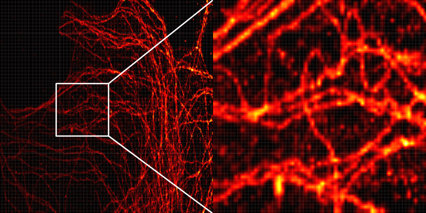
Single Marker Switching (SMS) Microscopy (Betzig et al.,, 2006; Rust et al.,, 2006; Egner et al.,, 2007; Heilemann et al.,, 2008; Fölling et al.,, 2008) is a living cell fluorescence microscopy technique in which fluorescent markers which are tagged to a protein structure in the probe are stochastically switched from a no-signal giving (off) state into a signal-giving (on) state. A marker in the on state emits a bunch of photons some of which are detected on a detector before it is either switched off or bleached. From the photons registered on the detector, the position of the marker (and hence of the protein) can be determined. The final image is assembled from all observed individual positions recorded in a sequence of time intervals (frames) in a position histogram, typically a pixel grid.

SMS microscopy is based on the principle that at any given time only a very small number of markers are in the on state. As the probability of switching from the off to the on state is small for each individual marker and they remain in the on state only for a very short time (1-100ms). This allows SMS microscopy to resolve features below the diffraction barrier that limits conventional far-field microscopy (see Hell, (2007) for a survey) because with overwhelming probability at most one marker within a diffraction limited spot is in the on state (Aspelmeier et al.,, 2015). At the same time this requires quite long acquisition times (1min-1h) to guarantee sufficient sampling of the probe. As a consequence, if the probe moves during the acquisition, the final image will be blurred.

Correcting for this drift and thus improving image quality is an area of active research (Geisler et al.,, 2012; Deschout et al.,, 2014; Hartmann et al.,, 2016). In order to investigate the validity of such a drift correction method we introduce a test of the Wasserstein distance between the image obtained from the first half of the recording time and the second half. This test is based on the distributional upper bound of the limiting distribution which was developed in Section 3.2 in combination with a lower bound of the Wasserstein distance (Pele and Werman,, 2009). In fact, there is no standard method for problems of this kind and we argue that the (thresholded) Wasserstein distance is particular useful in such a situation as the specimen moves between the frames without loss of mass, hence the drift induces a transport structure between successive frames. In the following we compare the distribution from the first half of frames with the distribution from the second half scaled with the sample sizes (as in (21)). We reject the hypothesis that the distributions from the first and the second half are the same, if our test statistic is larger than the $1-\alpha$ quantile of the distributional bound of the limiting distribution in (23). If we have statistical evidence that the thresholded Wasserstein distance is not zero, we can also conclude that there is a significant difference in the Wasserstein distance itself.

Statistical Model

It is common to assume the bursts of photons registered on the detector as independent realizations of a random variable with a density that is proportional to the density of markers in the probe (Aspelmeier et al.,, 2015). As it is expected that the probe drifts during the acquisition this density will vary over time. In particular, the positions registered at the beginning of the observation will follow a different distribution than those observed at the end.

Data and Results

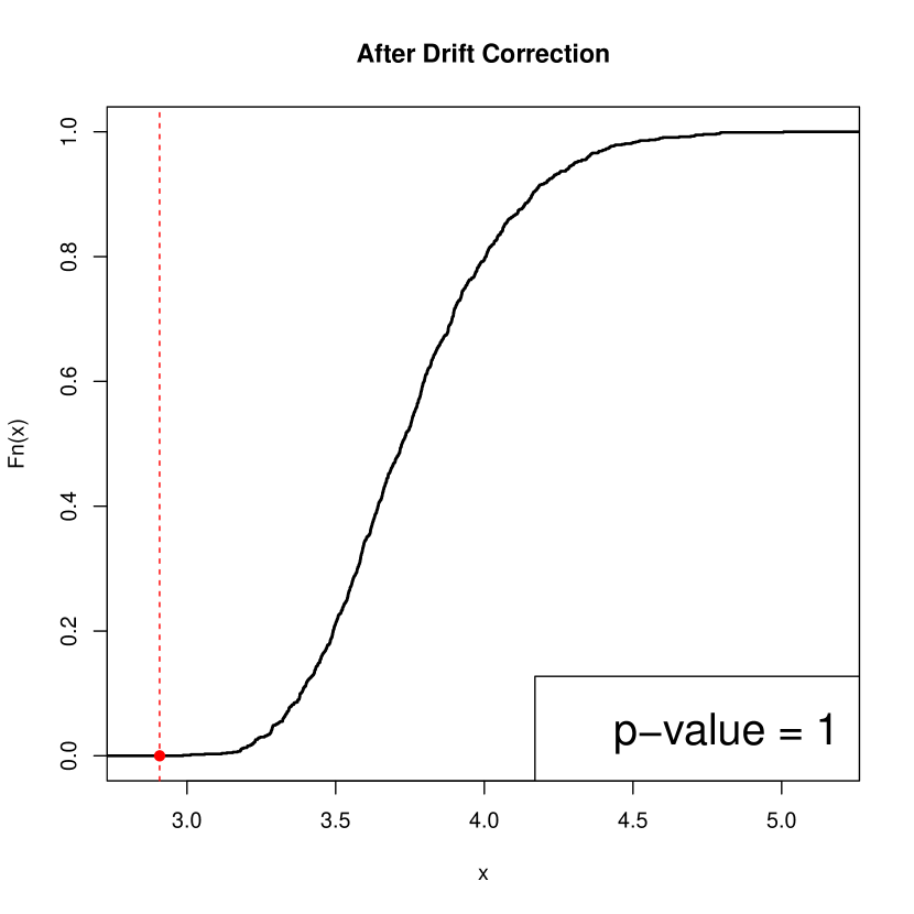
We consider an SMS image of a tubulin structure presented in Hartmann et al., (2016) to assess their drift correction method. This image is recorded in 40.000 single frames over a total recording time of 10 minutes (i.e., 15 ms per frame). We compare the aggregated sample collected during the first $50\%$ ($\hat{=}$ 20.000 frames) of the total observation time with the aggregated sample obtained in the last $50\%$ on a $256\times 256$ grid for both the original uncorrected values and for the values where the drift correction of Hartmann et al., (2016) was applied. Heat maps of these four samples are shown in the left hand side of Figure 2 (no correction) and Figure 3 (corrected), respectively.

   

Figure 2: Left: Aggregated samples of the first (first row) and the last (second row) $50\%$ of the observation time as heat maps of relative frequency without correction for the drift of the probe. Magnifications of a small area are shown to highlight the blurring of the picture. Right: Empirical distribution function of a sample from the upper bound (tree approximation) of the limiting distribution. The red dot (line) indicates the scaled thresholded Wasserstein distance for $t=6/256$.

   

Figure 3: Left: Aggregated samples of the first (first row) and the last (second row) $50\%$ of the observation time as heat maps of relative frequency with correction for the drift of the probe. Magnifications of a small area are shown to highlight the drift correction of the picture. Right: Empirical distribution function of a sample from the upper bound (tree approximation) of the limiting distribution. The red dot (line) indicates the scaled thresholded Wasserstein distance after drift correction for $t=6/256$. The difference between the fist and the second $50\%$ is no longer significant.

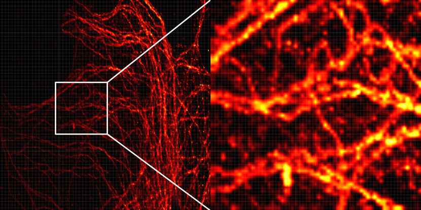
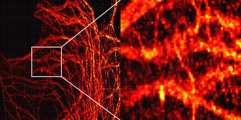
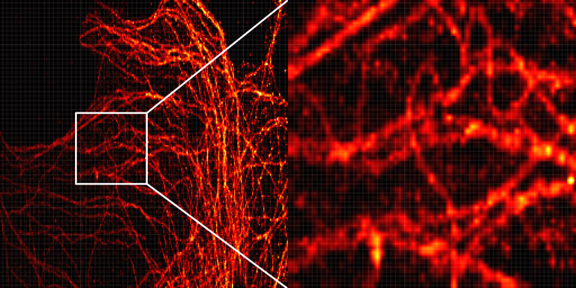
The question we will address is: ”To what extend has the drift been properly removed by the drift correction?” In addition, from the application of the thresholded Wasserstein distance for different thresholds we expect to obtain detailed understanding for which scales the drift has been removed. As Hartmann et al., (2016) have corrected with a global drift function one might expect that on small spatial scales not all effects have been removed.

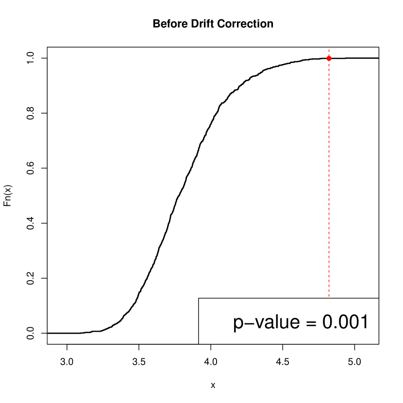
We compute the thresholded Wasserstein distance $W^{t}_{1}$ between the two pairs of samples as described in Section 4.1 with different thresholds $t\in\{2,3,\ldots,14\}/256$. We compare these values with a sample from the stochastic upper bound for the limiting distribution on regular grids obtained as described in Section 4.2. This allows us to obtain a test for the null hypothesis ’no difference’ based on Theorem 3.3. To visualize the outcomes of theses tests for different thresholds $t$ we have plotted the corresponding p-values in Figure 4. The red line indicates the magnitude of the drift over the total recording time. As the magnitude is approximately $6/256$, we plot in the right hand side of Figure 2 and Figure 3 the empirical distribution functions of the upper bound (23) and indicate the value of the test-statistic for $t=6/256$ with a red dot without the drift correction and with the correction, respectively.

Figure 4: P-values for the null hypothesis ’no difference’ for different thresholds $t$ before and after the drift correction. The red line indicates the magnitude of the total drift.

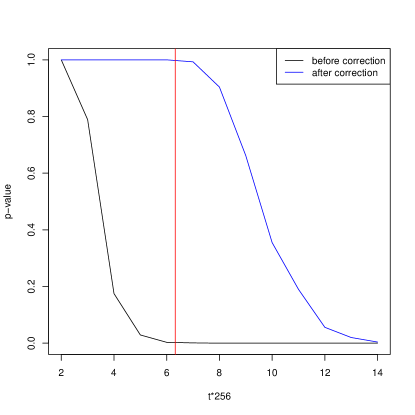
As shown in Figure 4 the differences caused by the drift of the probe are recognized as highly statistically significant ($p\leq 0.05$) for thresholds larger than $t=4/256$. After the drift correction method is applied, the difference is no longer significant for thresholds smaller than $t=14/256$. The estimated shift during the first and the second 50% of the observations is three pixels in x-direction and one pixel in y-direction. That shows that the significant difference that is detected when comparing the images without drift correction for $t\in\{5,6,7,8,9,10\}/256$ is caused in fact by the drift. The fact that there is still a significant difference for large thresholds ($t\geq 14$) in the corrected pictures suggests further intrinsic and local inhomogeneous motion of the specimen or non-polynomial drift that is not captured by the drift model used in Hartmann et al., (2016) and bleaching effects of fluorescent markers.

In summary, this example demonstrates that our strategy of combining a lower bound for the Wasserstein distance with a stochastic bound of the limiting distribution is capable of detecting subtle differences in a large $N$ setting.

Appendix A Proofs

A.1 Hadamard directional differentiability

In this section we follow mainly Shapiro, (1991) and Römisch, (2004). Let $\mathcal{U}$ and $\mathcal{Y}$ be normed spaces.

Definition A.1 (cf. Shapiro, (1991), Römisch, (2004)).

• Hadamard directional differentiability
  A mapping $f\colon D_{f}\subset\mathcal{U}\to\mathcal{Y}$ is said to be Hadamard directionally differentiable at $u\in\mathcal{U}$ if for any sequence $h_{n}$ that converges to $h$ and any sequence $t_{n}\searrow 0$ such that $u+t_{n}h_{n}\in D_{f}$ for all $n$ the limit

  $$f_{u}^{\prime}(h)=\lim_{n\to\infty}\frac{f(u+t_{n}h_{n})-f(u)}{t_{n}}$$ (29)

  exist.

• Hadamard directional differentiability tangentially to a set Let $K$ be a subset of $\mathcal{U}$, $f$ is directionally differentiable tangentially to $K$ in the sense of Hadamard at $u$ if the limit (29) exists for all sequences $h_{n}$ that converge to $h$ of the form $h_{n}=t_{n}^{-1}(k_{n}-u)$ where $k_{n}\in K$ and $t_{n}\searrow 0$. This derivative is defined on the contingent (Bouligand) cone to $K$ at $u$

  $$T_{K}(u)=\left\{h\in\mathcal{U}:h=\lim_{n\to\infty}t_{n}^{-1}(k_{n}-u),k_{n}\in K,t_{n}\searrow 0\right\}.$$

Note that this derivative is not required to be linear in $h$, but it is still positively homogeneous. Moreover, the directional Hadamard derivative $f_{u}^{\prime}(\cdot)$ is continuous if $u$ is an interior point of $D_{f}$ (Römisch,, 2004).

The delta method for mappings that are directionally Hadamard differentiable tangentially to a set reads as follows:

Theorem A.2 (Römisch, (2004), Theorem 1).

Let $K$ be a subset of $\mathcal{U}$, $f\colon K\to\mathcal{Y}$ a mapping and assume that the following two conditions are satisfied:

1. The mapping $f$ is Hadamard directionally differentiable at $u\in K$ tangentially to $K$ with derivative $f_{u}^{\prime}(\cdot)\colon T_{K}(u)\to\mathcal{Y}$.

2. For each $n$, $X_{n}\colon\Omega_{n}\to K$ are maps such that $a_{n}(X_{n}-u)\xrightarrow{\mathscr{D}}X$ for some sequence $a_{n}\to+\infty$ and some random element $X$ that takes values in $T_{K}(u)$.

Then we have $a_{n}(f(X_{n})-f(u))\xrightarrow{\mathscr{D}}f_{u}^{\prime}(X).$

Hadamard directional differentiability of the Wasserstein distance on countable metric spaces

For $\bm{r},\bm{s}\in\mathcal{P}_{p}(\mathcal{X})$ the $p$-th power of the $p$-th Wasserstein distance is the optimal value of an infinite dimensional linear program. We use this fact to verify that the $p$-th power of the Wasserstein distance (4) on the countable metric spaces $\mathcal{X}$ is directionally Hadamard differentiable with methods of sensitivity analysis of optimal values.

The $p$-th power of the Wasserstein distance on countable metric spaces is the optimal value of the following infinite dimensional linear program

$$\min_{\bm{w}\in\ell^{1}_{d^{p}}(\mathcal{X}\times\mathcal{X})} \sum_{x,x^{\prime}\in\mathcal{X}}d^{p}(x,x^{\prime})w_{x,x^{\prime}}$$ (30)

subject to $$\sum_{x^{\prime}\in\mathcal{X}}w_{x,x^{\prime}}=r_{x}\quad\forall x\in\mathcal{X},$$

$$\sum_{x\in\mathcal{X}}w_{x,x^{\prime}}=s_{x^{\prime}},\quad\forall x^{\prime}\in\mathcal{X},$$

$$w_{x,x^{\prime}}\geq 0,\quad\forall x,x^{\prime}\in\mathcal{X}.$$

Theorem A.3.

$W_{p}^{p}$ as a map from $(\mathcal{P}_{p}(\mathcal{X})\times\mathcal{P}_{p}(\mathcal{X}),\|\cdot\|_{\ell^{1}(d^{p})})$ to $\mathbb{R}$, $(\bm{r},\bm{s})\mapsto W_{p}^{p}(\bm{r},\bm{s})$ is Hadamard directionally differentiable tangentially to $\mathcal{P}_{p}(\mathcal{X})\times\mathcal{P}_{p}(\mathcal{X})$. The contingent cone on which the derivative is defined is given by

$$\mathcal{D}(\bm{r},\bm{s})=\mathcal{D}(\bm{r})\times\mathcal{D}(\bm{s})$$

with

$$\mathcal{D}(\bm{r})\mathrel{\mathop{:}}=\left\{\bm{d}\in\ell^{1}_{d^{p}}(\mathcal{X})\backslash\{0\}\colon\sum_{x\in\mathcal{X}}{d}_{x}=0,~{}d_{x}\in[-r_{x},1-r_{x}]\right\}$$

and the directional derivative is as follows

$$(\bm{d}_{1},\bm{d}_{2})\mapsto\sup_{(\bm{\lambda},\bm{\mu})\in\mathcal{S}^{*}(\bm{r},\bm{s})}-(\langle\bm{\lambda},\bm{d}_{1}\rangle+\langle\bm{\mu},\bm{d}_{2}\rangle),$$ (31)

where $\mathcal{S}^{*}(\bm{r},\bm{s})$ is set of optimal solutions of the dual problem which is defined in (6).

Proof.

We start the proof with stating the considered functions and the spaces on which they are defined. The objective function of the linear program that determines the $p$-th power of the $p$-th Wasserstein distance is given as $f\colon\ell^{1}_{d^{p}}(\mathcal{X}\times\mathcal{X})\to\mathbb{R},\bm{w}\mapsto\sum_{x,x^{\prime}\in\mathcal{X}}d^{p}(x,x^{\prime})w_{x,x^{\prime}}$. The constraints are encoded by the constraint function $C\colon\ell^{1}_{d^{p}}(\mathcal{X}\times\mathcal{X})\times\ell^{1}_{d^{p}}(\mathcal{X})\times\ell^{1}_{d^{p}}(\mathcal{X})\to\ell^{1}_{d^{p}}(\mathcal{X}\times\mathcal{X})\times\ell^{1}_{d^{p}}(\mathcal{X})\times\ell^{1}_{d^{p}}(\mathcal{X})$ with

$$C(\bm{w},(\bm{r},\bm{s}))=\begin{pmatrix}\bm{w}\\ \Sigma_{1}\bm{w}-\bm{r}\\ \Sigma_{2}\bm{w}-\bm{s}\\ \end{pmatrix},$$ (32)

here $\Sigma_{1},\Sigma_{2}\colon\ell^{1}_{d^{p}}(\mathcal{X}\times\mathcal{X})\to\ell^{1}_{d^{p}}(\mathcal{X})$ are the summation operators over the first and the second component, i.e., $\Sigma_{1}\bm{w}=\sum_{x^{\prime}\in\mathcal{X}}w_{x,x^{\prime}}$ and $\Sigma_{2}\bm{w}=\sum_{x\in\mathcal{X}}w_{x,x^{\prime}}$. Furthermore, we need the closed convex set $K=\ell^{1}_{d^{p}}(\mathcal{X}\times\mathcal{X})_{+}\times\left\{\bm{0}\right\}\times\left\{\bm{0}\right\}$ were $\ell^{1}_{d^{p}}(\mathcal{X}\times\mathcal{X})_{+}$ are the elements in $\ell^{1}_{d^{p}}(\mathcal{X}\times\mathcal{X})$ that have only non-negative entries. With these definitions the $p$-th power of the $p$-th Wasserstein distance is the optimal value of the following abstract parametrized optimization problem:

$$\min_{\bm{w}\in\ell^{1}_{d^{p}}(\mathcal{X}\times\mathcal{X})}f(\bm{w})\text{ s.t. }C(\bm{w},(\bm{r},\bm{s}))\in K$$ (33)

We will use Theorem 4.24 from Bonnans and Shapiro, (2000). To this end, we need to check the following three conditions.

• Convexity and existence of optimal solution
  Problem (30) is obviously convex as it is a linear program with linear constraints. Note that the definition of a convex problem (Def. 2.163) in Bonnans and Shapiro, (2000) is slightly different from the usual definition of a convex program as they require convexity of the constraint function (32) with respect to $-K$. This condition can be shown by easy calculations for our problem.
  The set of primal optimal solutions, $\mathcal{S}(\bm{r},\bm{s})$, is according to Thm. 4.1 in Villani, (2008) non empty.

• Directional regularity
  Set for some direction $(\bm{d}_{1},\bm{d}_{2})\in\mathcal{D}(\bm{r},\bm{s})\subset\ell^{1}_{d^{p}}(\mathcal{X})\times\ell^{1}_{d^{p}}(\mathcal{X})$

  $$\bar{C}(\bm{w},t)=(\bm{w},\bm{w}^{T}\mathds{1}-\bm{r}-t\bm{d}_{1},\bm{w}\mathds{1}-\bm{s}-t\bm{d}_{2},t).$$

  The directional regularity condition is fulfilled at $\bm{w}_{0}$ in a direction $(\bm{d}_{1},\bm{d}_{2})$ if Robinson’s constraint qualification is satisfied at the point $(\bm{w}_{0},0)$ for the mapping $\bar{C}(\bm{w},t)$ with respect to the set $K\times\mathbb{R}_{+}$ (Bonnans and Shapiro,, 2000, Def. 4.8). According to Thm. 4.9 in Bonnans and Shapiro, (2000) the following condition is necessary and sufficient for the directional regularity constraint to hold:

  $$\bm{0}\in int\left\{C(\bm{w}_{0},(\bm{r},\bm{s}))+DC(\bm{w},(\bm{r},\bm{s}))(\ell^{1}_{d^{p}}(\mathcal{X}\times\mathcal{X}),\mathbb{R}_{+}(\bm{d}_{1},\bm{d}_{2}))-K\right\},$$

  where $\mathbb{R}_{+}(\bm{d}_{1},\bm{d}_{2})=\left\{t(\bm{d}_{1},\bm{d}_{2}),t\geq 0\right\}$. We are going to show that the directional regularity condition in a direction $(\bm{d}_{1},\bm{d}_{2})\in\mathcal{D}(\bm{r},\bm{s})$ holds for all primal optimal solutions $\bm{w}_{0}\in\mathcal{S}(\bm{r},\bm{s})$.
  For a primal optimal solution $\bm{w}_{0}$ it is

  $$C(\bm{w}_{0},(\bm{r},\bm{s}))=(\bm{w}_{0},\bm{0},\bm{0}).$$

  Since $C(\bm{w},(\bm{r},\bm{s}))$ is linear in $(\bm{w},(\bm{r},\bm{s}))$ and bounded with respect to the product norm on the space $\ell^{1}_{d^{p}}(\mathcal{X}\times\mathcal{X})\times\ell^{1}_{d^{p}}(\mathcal{X})\times\ell^{1}_{d^{p}}(\mathcal{X})$ it holds that
  $DC(\bm{w}_{0},(\bm{r},\bm{s}))(\ell^{1}_{d^{p}}(\mathcal{X}\times\mathcal{X}),\mathbb{R}_{+}(\bm{d}_{1},\bm{d}_{2}))=(\bm{w},\Sigma_{1}\bm{w}-t\bm{d}_{1},\Sigma_{2}\bm{w}-t\bm{d}_{2})$ for $t\geq 0$ and the directional regularity condition reads

  $$\bm{0}\in int\left\{(\bm{w}_{0},\bm{0},\bm{0})+(\bm{w},\Sigma_{1}\bm{w}-t\bm{d}_{1},\Sigma_{2}\bm{w}-t\bm{d}_{2})-K\right\}.$$

  This set is just $\ell^{1}_{d^{p}}(\mathcal{X}\times\mathcal{X})\times\ell^{1}_{d^{p}}(\mathcal{X})\times\ell^{1}_{d^{p}}(\mathcal{X})$ as $\bm{w}\in\ell^{1}_{d^{p}}(\mathcal{X}\times\mathcal{X})$ and hence the directional regularity constraint is fulfilled.
  

• Stability of primal optimal solution
  We aim to verify that for perturbed measures of the form $\bm{r}_{n}=\bm{r}+t_{n}\bm{d}_{1}+o(t_{n})$ and $\bm{s}_{n}=\bm{s}+t_{n}\bm{d}_{2}+o(t_{n})$ with $t_{n}\searrow 0$, $\bm{r},\bm{s}\in\mathcal{P}_{p}(\mathcal{X})$, $\bm{d}_{1}\in\mathcal{D}(\bm{r})$ and $\bm{d}_{2}\in\mathcal{D}(s)$ there exist a sequence of primal optimal solutions $\bm{w}_{n}$ that converges to the primal optimal solution $\bm{w}_{0}$ of the unperturbed problem. For $n$ large enough $t_{n}\leq 1$, hence we can assume without loss of generality that $t_{n}\leq 1$ for all n. In this case $\bm{r}_{n}$ and $\bm{s}_{n}$ are probability measure with existing $p$-th moment, i.e. elements of $\mathcal{P}_{p}(\mathcal{X})$. This yields that Theorem 5.20 in Villani, (2008) is applicable. This theorem gives us the stability of the optimal solution as $\mathcal{P}_{p}(\mathcal{X})$ is a closed subset of $\ell^{1}_{d^{p}}(\mathcal{X})$.

So far, we checked all the assumptions of Theorem 4.24 in Bonnans and Shapiro, (2000). The rest of this section is devoted to the derivation of formula (31) from the result of that theorem.
The Lagrangian $L$ of a parametrized optimization problem

$$\min_{w}f(w,u)\text{ s.t. }C(w,u)\in K$$

is given by

$$L(w,\lambda,u)=f(w,u)+\langle\lambda,C(w,u)\rangle,$$

where $f$ is the objective function, $u$ the parameter and $C$ the constraint function and $\langle\cdot,\cdot\rangle$ the dual pairing (see for example Section 2.5.2 in Bonnans and Shapiro, (2000)). We refer to $\lambda$ as Lagrange multiplier. For the transport problem this yields with $(\bm{r},\bm{s})$ being the parameter and the definition of the constraint function in (32)

$$L(\bm{w},(\bm{\nu},\bm{\lambda},\bm{\mu}),(\bm{r},\bm{s}))\\ =\sum_{x,x^{\prime}\in\mathcal{X}}d^{p}(x,x^{\prime})w_{x,x^{\prime}}+\langle\bm{\nu},\bm{w}\rangle+\langle\bm{\lambda},\bm{w}^{T}\mathds{1}-\bm{r}\rangle+\langle\bm{\mu},\bm{w}\mathds{1}-\bm{s}\rangle.$$

Differentiating this in the Fréchet sense with respect to $(\bm{r},\bm{s})$ and applying $(\bm{d}_{1},\bm{d}_{2})$ to this linear operator results in

$$D_{(r,s)}L(\bm{w},(\bm{\nu},\bm{\lambda},\bm{\mu}),(\bm{r},\bm{s}))(\bm{d}_{1},\bm{d}_{2})=-(\langle\bm{\lambda},\bm{d}_{1}\rangle+\langle\bm{\mu},\bm{d}_{2}\rangle)$$

as the Lagrangian is linear and bounded in $(\bm{r},\bm{s})$. As this derivative is independent of $\bm{w}$ and the set of Lagrange multipliers $\Lambda(\bm{r},\bm{s})$ equals the set of dual solutions $\mathcal{S}^{*}(\bm{r},\bm{s})$ in the case of a convex unperturbed problem (see section above Thm. 4.24 in Bonnans and Shapiro, (2000)) it holds that the directional Hadamard derivative is given by

$$(\bm{d}_{1},\bm{d}_{2})\mapsto\inf_{\bm{w}\in\mathcal{S}(\bm{r},\bm{s})}\sup_{(\bm{\lambda},\bm{\mu})\in\Lambda(\bm{r},\bm{s})}D_{(r,s)}L(\bm{w},(\bm{\nu},\bm{\lambda},\bm{\mu}),(\bm{r},\bm{s}))(\bm{d}_{1},\bm{d}_{2})\\ =\inf_{\bm{w}\in\mathcal{S}(\bm{r},\bm{s})}\sup_{(\bm{\lambda},\bm{\mu})\in\Lambda(\bm{r},\bm{s})}-(\langle\bm{\lambda},\bm{d}_{1}\rangle+\langle\bm{\mu},\bm{d}_{2}\rangle)\\ =\sup_{(\bm{\lambda},\bm{\mu})\in\mathcal{S}^{*}(\bm{r},\bm{s})}-(\langle\bm{\lambda},\bm{d}_{1}\rangle+\langle\bm{\mu},\bm{d}_{2}\rangle).$$

∎

A.2 The limit distribution under equality of measures

First, observe that for the case $\bm{r}=\bm{s}$ the set of dual solutions $\mathcal{S}^{*}(\bm{r},\bm{r})$ in (6) reduces to:

$$\mathcal{S}^{*}(\bm{r},\bm{r}) =\Big{\{}(\bm{\lambda},\bm{\mu})\in\ell^{\infty}_{d^{-p}}(\mathcal{X})\times\ell^{\infty}_{d^{-p}}(\mathcal{X}):\left\langle\bm{r},\bm{\lambda}\right\rangle+\left\langle\bm{r},\bm{\mu}\right\rangle=0,$$

$$\hskip 150.69397pt\lambda_{x}+\mu_{x^{\prime}}\leq d^{p}(x,x^{\prime})\quad\forall x,x^{\prime}\in\mathcal{X}\Big{\}}$$

$$=\Big{\{}(\bm{\lambda},\bm{\mu})\in\ell^{\infty}_{d^{-p}}(\mathcal{X})\times\ell^{\infty}_{d^{-p}}(\mathcal{X}):\lambda_{x}=-\mu_{x}\text{ for }x\in\mathrm{supp}(\bm{r}),$$

$$\hskip 150.69397pt\lambda_{x}+\mu_{x^{\prime}}\leq d^{p}(x,x^{\prime})\quad\forall x,x^{\prime}\in\mathcal{X}\Big{\}}.$$

The equality follows as for $x=x^{\prime}$ the inequality condition gives $\lambda_{x}+\mu_{x}\leq 0$ and all $r_{x}$ in the sum are non-negative. The conjunction of these two conditions yields $\lambda_{x}+\mu_{x}=0$.
This set is a subset of the set given in (7), but changing $\mathcal{S}^{*}(r,r)$ to $\mathcal{S}^{*}(r)$ does not change the optimal value of the linear programs in Theorem 2.1 and 2.4 as the Gaussian process $\mathbf{G}$ is zero at all $x\notin\mathrm{supp}(\bm{r})$.
In the case, that the support of $\bm{r}$, i.e., $\left\{x\in\mathcal{X}\colon r_{x}>0\right\}$, is the whole ground space $\mathcal{X}$, the set $\mathcal{S}^{*}(\bm{r})$ is independent of $\bm{r}$ and it reduces to

$$\mathcal{S}^{*}=\Big{\{}\bm{\lambda}\in\ell^{\infty}_{d^{-p}}(\mathcal{X}):\lambda_{x}-\lambda_{x^{\prime}}\leq d^{p}(x,x^{\prime})\quad\forall x,x^{\prime}\in\mathcal{X}\Big{\}}.$$

Proof of Thm. 2.4 a).

For the two sample case the delta method together with the continuous mapping theorem and equation (14) gives

$$\rho_{n,m}^{1/p}W_{p}(\hat{\mathbf{r}}_{n},\hat{\mathbf{s}}_{m})\xrightarrow{\mathscr{D}}\left\{\max_{(\bm{\lambda},\bm{\mu})\in\mathcal{S}^{*}(\bm{r},\bm{r})}\sqrt{\alpha}\langle\bm{\lambda},\mathbf{G}\rangle+\sqrt{1-\alpha}\langle\bm{\mu},\mathbf{G}^{\prime}\rangle\right\}^{1/p}.$$

Nevertheless, for all $x\in\mathcal{X}$ where $r_{x}>0$ it holds $\lambda_{x}=-\mu_{x}$ and for all $x\in\mathcal{X}$ where $r_{x}=0$ the limit element $G_{x}$ is degenerate. Hence, the limit distribution above is equivalent in distribution to

$$\left\{\max_{\bm{\lambda}\in\mathcal{S}^{*}(\bm{r},\bm{r})}\sqrt{\alpha}\langle\bm{\lambda},\mathbf{G}\rangle-\sqrt{1-\alpha}\langle\bm{\lambda},\mathbf{G}^{\prime}\rangle\right\}^{1/p}.$$

The independence of $\mathbf{G}$ and $\mathbf{G}^{\prime}$ yield that $\sqrt{\alpha}\langle\bm{\lambda},\mathbf{G}\rangle-\sqrt{1-\alpha}\langle\bm{\lambda},\mathbf{G}^{\prime}\rangle$ equals $\sqrt{\alpha+(1-\alpha)}\langle\bm{\lambda},\mathbf{G}\rangle$ in distribution and hence the limit reduces to

$$\left\{\max_{\bm{\lambda}\in\mathcal{S}^{*}(\bm{r})}\langle\bm{\lambda},\mathbf{G}\rangle\right\}^{1/p}.$$

∎

Proof of decomposition in Rem. 2.3 e).

For the alternative representation of the distributional limit we decompose the Gaussian process $\mathbf{G}$ with mean zero and covariance structure as defined in (8) into $\mathbf{G}=\mathbf{G}^{+}-\mathbf{G}^{-}$ with $\mathbf{G}^{+}$, $\mathbf{G}^{-}$ non-negative, then the limiting distribution in (9) can be rewritten as follows:

$$\max_{\bm{\lambda}\in\mathcal{S}^{*}(\bm{r})}\langle\mathbf{G},\bm{\lambda}\rangle =\max_{\bm{\lambda}\in\mathcal{S}^{*}(\bm{r},\bm{r})}\langle\mathbf{G}^{+},\bm{\lambda}\rangle-\langle\mathbf{G}^{-},\bm{\lambda}\rangle$$

$$=\max_{(\bm{\lambda},\bm{\mu})\in\ell^{\infty}_{d^{-p}}(\mathcal{X})\times\ell^{\infty}_{d^{-p}}(\mathcal{X})}\langle\mathbf{G}^{+},\bm{\lambda}\rangle+\langle\mathbf{G}^{-},\bm{\mu}\rangle$$

$$~{}\text{s.t.}\quad\lambda_{x}+\mu_{x}=0\quad\text{for all}\quad x\in\mathrm{supp}(\bm{r})$$

$$\lambda_{x}+\mu_{x^{\prime}}\leq d^{p}(x,x^{\prime})\quad\forall x,x^{\prime}\in\mathcal{X}.$$

The Lagrangian for this problem is given by

$$L(\bm{\lambda},\bm{\mu},\bm{w},\bm{z})=\sum_{x\in\mathcal{X}}{G^{+}_{x}\lambda_{x}}+\sum_{x^{\prime}\in\mathcal{X}}{G^{-}_{x^{\prime}}\mu_{x^{\prime}}}\\ +\sum_{x\in\mathcal{X}}{z_{x}(\lambda_{x}+\mu_{x})\mathds{1}_{\{r_{x}>0\}}}+\sum_{x,x^{\prime}\in\mathcal{X}}{w_{x,x^{\prime}}(\lambda_{x}+\mu_{x^{\prime}}-d^{p}(x,x^{\prime}))}.$$

From this we can derive the dual via

$$\min_{\bm{w}\geq 0\in\ell^{1}_{d^{p}}(\mathcal{X}\times\mathcal{X}),\bm{z}\in\ell^{1}_{d^{p}}(\mathcal{X})}\sup_{\bm{\lambda},\bm{\mu}\in\ell^{\infty}_{d^{-p}}(\mathcal{X})}L(\bm{\lambda},\bm{\mu},\bm{w},\bm{z}),$$

where $\bm{w}\geq 0$ to be understood componentwise. It yields

$$\inf_{\bm{w}\geq 0,\bm{z}} \sum_{x,x^{\prime}\in\mathcal{X}}d^{p}(x,x^{\prime})w_{x,x^{\prime}}$$

s.t. $$\sum_{x^{\prime}\in\mathcal{X}}w_{x,x^{\prime}}=G^{+}_{x}+z_{x}\mathds{1}_{\{r_{x}>0\}}$$

$$\sum_{x\in\mathcal{X}}w_{x,x^{\prime}}=G^{-}_{x^{\prime}}+z_{x^{\prime}}\mathds{1}_{\{r_{x}>0\}},$$

where the minimum over $\bm{w}$ equals the $p$-th power of the $p$-th Wasserstein distance. More precisely the linear program above is equivalent to

$$\inf_{\bm{z}(\bm{r})\in\ell^{1}_{d^{p}}(\mathcal{X})}W_{p}^{p}\left(\mathbf{G}^{+}+\bm{z}(\bm{r}),\mathbf{G}^{-}+\bm{z}(\bm{r})\right),$$

where $\bm{z}(\bm{r})$ depends on $\bm{r}$ through the support of $\bm{r}$ in the following sense: $z_{x}=0$ for $x\in\mathcal{X}$ such that $r_{x}=0$. ∎

A.3 Proof of Theorem 3.1

Simplify the set of dual solutions $\mathcal{S}^{*}$

As a first step, we rewrite the set of dual solutions $\mathcal{S}^{*}$ given in definition (11) in our tree notation as

$$\mathcal{S}^{*}=\left\{\bm{\lambda}\in\ell^{\infty}_{d^{-p}}(\mathcal{X}):\lambda_{x}-\lambda_{x^{\prime}}\leq d_{\mathcal{T}}(x,x^{\prime})^{p},\quad x,x^{\prime}\in\mathcal{X}\right\}.$$ (34)

The key observation is that in the condition $\lambda_{x}-\lambda_{x^{\prime}}\leq d_{\mathcal{T}}(x,x^{\prime})^{p}$ we do not need to consider all pairs of vertices $x,x^{\prime}\in\mathcal{X}$, but only those which are joined by an edge. To see this, assume that only the latter condition holds. Let $x,x^{\prime}\in\mathcal{X}$ arbitrary and $x=x_{1},\dots,x_{n}=x^{\prime}$ the sequence of vertices defining the unique path joining $x$ and $x^{\prime}$, such that $(x_{j},x_{j+1})\in E$ for $j=1,\dots,n-1$. That this path contains only a finite number of edges, was proven in Section 3. Then

$$\lambda_{x}-\lambda_{x^{\prime}}=\sum_{j=1}^{n-1}(\lambda_{x_{j}}-\lambda_{x_{j+1}})\leq\sum_{j=1}^{n-1}d_{\mathcal{T}}(x_{j},x_{j+1})^{p}\leq d_{\mathcal{T}}(x,x^{\prime})^{p},$$

such that (34) is satisfied for all $x,x^{\prime}\in\mathcal{X}$. Noting that if two vertices are joined by an edge then one has to be the parent of the other, we can write the set of dual solutions as

$$\mathcal{S}^{*}=\left\{\bm{\lambda}\in\ell^{\infty}_{d^{-p}}(\mathcal{X}):|\lambda_{x}-\lambda_{{\mathrm{parent}}(x)}|\leq d_{\mathcal{T}}(x,{\mathrm{parent}}(x))^{p},\quad x\in\mathcal{X}\right\}.$$ (35)

Rewrite the target function

To rewrite the target function we need to make several definitions. Let

$$\tilde{e}^{(x)}_{y}=\begin{cases}\frac{1}{d^{p}(x,x_{0})}&\text{ if }y=x,\\ -\frac{1}{d^{p}(x,x_{0})}&\text{ if }y={\mathrm{parent}}(x),\\ 0&\text{ else.}\end{cases}$$

Furthermore, we define for $\bm{\mu}\in\ell^{1}_{d^{p}}(\mathcal{X})$

$$\eta_{x}=\sum_{x^{\prime}\in{\mathrm{children}}(x)}d^{p}(x,x_{0})\mu_{x^{\prime}}$$

and

$$\bm{\mu}_{n} =\sum_{x\in A_{\leq n}\setminus{\mathrm{root}}(\mathcal{T})}\eta_{x}\tilde{\bm{e}}^{(x)}=\bm{\mu}\mathds{1}_{A_{<n}}+\sum_{x\in A_{=n}}\frac{1}{d^{p}(x,x_{0})}\eta_{x}\bm{e}{(x)},$$

here $A_{\leq n}=\left\{x\in\mathcal{X}\colon\text{level of }x\leq n,x\text{ is within the first }n\text{ vertices of its level}\right\}$,
$A_{=n}=\left\{x\in\mathcal{X}\colon\text{level of }x=n,x\text{ is within the first }n\text{ vertices of its level}\right\}$,
$A_{>n}=\left\{x\in\mathcal{X}\colon\text{level of }x>n\text{ or }x\text{ is not within the first }n\text{ vertices of its level}\right\}$ and $\bm{e}{(x)}$ the sequence 1 at $x$ and 0 everywhere else. For this sequence $\bm{\mu}_{n}$ it holds

$$\|\bm{\mu}-\bm{\mu}_{n}\|_{\ell^{1}(d^{p})} =\sum_{x\in X}d^{p}(x,x_{0})\left|\bm{\mu}\mathds{1}_{A_{>n}}-\sum_{\tilde{x}\in A_{=n}}\frac{1}{d^{p}(\tilde{x},x_{0})}\eta_{\tilde{x}}\bm{e}^{(\tilde{x})}\right|_{x}$$

$$\leq\|\bm{\mu}\mathds{1}_{A_{>n}}\|_{\ell^{1}(d^{p})}+\left|\sum_{x\in A_{=n}}\eta_{x}\right|.$$

As $n\to\infty$, the first part tends to zero as $\bm{\mu}\in\ell^{1}_{d^{p}}(\mathcal{X})$, and

$$\left|\sum_{x\in A_{=n}}\eta_{x}\right|\leq\sum_{x\in A_{=n}}\sum_{x^{\prime}\in{\mathrm{children}}(x)}\left|\mu_{x^{\prime}}\right|d^{p}(x^{\prime},x_{0})\leq\sum_{x\in A_{\geq n}}\left|\mu_{x}\right|d^{p}(x,x_{0})\xrightarrow{n\to\infty}0.$$

Hence, our target function for $\bm{\mu}\in\ell^{1}_{d^{p}(\mathcal{X})}$ and $\bm{\lambda}\in\ell^{\infty}_{d^{-p}}(\mathcal{X})$ can be rewritten in the following way

$$\langle\bm{\mu},\bm{\lambda}\rangle =\lim_{n\to\infty}\langle\bm{\mu}_{n},\bm{\lambda}\rangle$$ (36)

$$=\lim_{n\to\infty}\sum_{x\in A_{\leq n}}\eta_{x}\langle\tilde{\bm{e}}^{(x)},\bm{\lambda}\rangle$$

$$=\lim_{n\to\infty}\sum_{x\in A_{\leq n}}\sum_{x^{\prime}\in{\mathrm{children}}(x)}\mu_{x^{\prime}}(\lambda_{x}-\lambda_{{\mathrm{parent}}(x)})$$

$$\leq\lim_{n\to\infty}\sum_{x\in A_{\leq n}}\left|\sum_{x^{\prime}\in{\mathrm{children}}(x)}\mu_{x^{\prime}}\right|\left|\lambda_{x}-\lambda_{{\mathrm{parent}}(x)}\right|$$

$$=\lim_{n\to\infty}\sum_{x\in A_{\leq n}}\left|(S_{\mathcal{T}}\bm{\mu})_{x}\right|\left|\lambda_{x}-\lambda_{{\mathrm{parent}}(x)}\right|$$

Observe that for $\bm{\lambda}\in\mathcal{S}^{*}$ it holds

$$\left|\lambda_{x}-\lambda_{{\mathrm{parent}}(x)}\right|\leq d^{P}(x,{\mathrm{parent}}(x)).$$ (37)

By condition (3) $\bm{G}\sim\mathcal{N}(0,\Sigma(\bm{r}))$ is an element of $\ell^{1}_{d^{p}}(\mathcal{X})$. For $\bm{\lambda}\in\mathcal{S}^{*}$ we get with (36) and (37) that

$$\langle\bm{G},\bm{\lambda}\rangle\leq\lim_{n\to\infty}\sum_{x\in A_{\leq n}}\left|(S_{\mathcal{T}}\mathbf{G})_{x}\right|d_{\mathcal{T}}(x,{\mathrm{parent}}(x))^{p}.$$ (38)

Therefore, $\max_{\bm{\lambda}\in\mathcal{S}^{*}}\langle\bm{G},\bm{\lambda}\rangle$ is bounded by $\lim_{n\to\infty}\sum_{x\in A_{\leq n}}|(S_{\mathcal{T}}\bm{G})_{x}|d_{\mathcal{T}}(x,{\mathrm{parent}}(x))^{p}$. We can define the sequence $\bm{\nu}\in\ell^{\infty}_{d^{-p}}(\mathcal{X})$ by

$$\nu_{{\mathrm{root}}} =0$$ (39)

$$\nu_{x}-\nu_{{\mathrm{parent}}(x)} =\mathrm{sign}((S_{\mathcal{T}}\mathbf{G})_{x})d_{\mathcal{T}}(x,{\mathrm{parent}}(x))^{p}$$

From (35) and the fact that $d^{p}(x,{\mathrm{parent}}(x))\leq d^{p}(x,{\mathrm{root}}(\mathcal{T}))$ we see that $\bm{\nu}\in\mathcal{S}^{*}$ and by plugging $\bm{\nu}$ into equation (38) we can conclude that $\langle\bm{G},\bm{\nu}\rangle$ attains the upper bound in (38).
As the last step of our proof, we verify that the limit in (38) exists. Therefore, we rewrite condition (3) in terms of the edges and recall that $x_{0}={\mathrm{root}}(\mathcal{T})$.

$$\sum_{x\in\mathcal{X}}d_{\mathcal{T}}(x,x_{0})^{p}\sqrt{r_{x}}\geq\sum_{x\in\mathcal{X}}\sum_{x^{\prime}\in{\mathrm{children}}(x)}d_{\mathcal{T}}(x,{\mathrm{parent}}(x))^{p}\sqrt{r_{x^{\prime}}}.$$ (40)

The first moment of the limiting distribution can be bounded in the following way:

$$\mathds{E}\left[\sum_{x\in\mathcal{X}\setminus\{{\mathrm{root}}(\mathcal{T})\}}|(S_{\mathcal{T}}\bm{G})_{x}|d_{\mathcal{T}}(x,{\mathrm{parent}}(x))^{p}\right]$$

$$\qquad\leq\sum_{x\in\mathcal{X}}d_{\mathcal{T}}(x,{\mathrm{parent}}(x))^{p}\sqrt{(S_{\mathcal{T}}r)_{x}(1-(S_{\mathcal{T}}r)_{x})}$$

$$\qquad\leq\sum_{x\in\mathcal{X}}\sum_{x^{\prime}\in{\mathrm{children}}(x)}d_{\mathcal{T}}(x,{\mathrm{parent}}(x))^{p}\sqrt{r_{x^{\prime}}}$$

$$\qquad<\infty$$

due to Hölder’s inequality and (40). This bound shows that the limit in (38) is almost surely finite and hence, concludes the proof.

References

- Ajtai et al., (1984) Ajtai, M., Komlós, J., and Tusnády, G. (1984). On optimal matchings. Combinatorica, 4(4):259–264.
- Aspelmeier et al., (2015) Aspelmeier, T., Egner, A., and Munk, A. (2015). Modern statistical challenges in high-resolution fluorescence microscopy. Annu. Rev. Stat. Its Appl., 2(1):163–202.
- Barbour and Brown, (1992) Barbour, A. D. and Brown, T. C. (1992). Stein’s method and point process approximation. Stochastic Process. Appl., 43(1):9–31.
- Bertsekas, (1981) Bertsekas, D. P. (1981). A new algorithm for the assignment problem. Mathematical Programming, 21(1):152–171.
- Bertsekas, (1992) Bertsekas, D. P. (1992). Auction algorithms for network flow problems: A tutorial introduction. Comput. Optim. Appl., 1(1):7–66.
- Bertsekas, (2009) Bertsekas, D. P. (2009). Auction algorithms. In Encyclopedia of Optimization, pages 128–132. Springer.
- Betzig et al., (2006) Betzig, E., Patterson, G. H., Sougrat, R., Lindwasser, O. W., Olenych, S., Bonifacino, J. S., Davidson, M. W., Lippincott-Schwartz, J., and Hess, H. F. (2006). Imaging intracellular fluorescent proteins at nanometer resolution. Science, 313(5793):1642–1645.
- Bickel and Freedman, (1981) Bickel, P. J. and Freedman, D. A. (1981). Some asymptotic theory for the bootstrap. Ann. Statist., 9(6):1196–1217.
- Bobkov and Ledoux, (2014) Bobkov, S. and Ledoux, M. (2014). One-dimensional empirical measures, order statistics and Kantorovich transport distances. Preprint.
- Boissard and Gouic, (2014) Boissard, E. and Gouic, T. L. (2014). On the mean speed of convergence of empirical and occupation measures in Wasserstein distance. Ann. Inst. H. Poincaré Probab. Statist., 50(2):539–563.
- Bonnans and Shapiro, (2000) Bonnans, J. F. and Shapiro, A. (2000). Perturbation Analysis of Optimization Problems. Springer, New York, NY.
- Bonneel et al., (2015) Bonneel, N., Rabin, J., Peyré, G., and Pfister, H. (2015). Sliced and Radon Wasserstein barycenters of measures. J. Math. Imaging Vis., 51(1):22–45.
- Cuturi, (2013) Cuturi, M. (2013). Sinkhorn distances: Lightspeed computation of optimal transport. In Advances in Neural Information Processing Systems, pages 2292–2300.
- de Wet and Venter, (1972) de Wet, T. and Venter, J. H. (1972). Asymptotic distributions of certain test criteria of normality. South African Statist. J., 6(2):135–149.
- Dede, (2009) Dede, S. (2009). An empirical central limit theorem in for stationary sequences. Preprint. https://arxiv.org/abs/0812.2839.
- Dedecker and Merlevede, (2015) Dedecker, J. and Merlevede, F. (2015). Behavior of the Wasserstein distance between the empirical and the marginal distributions of stationary -dependent sequences. Preprint. https://arxiv.org/abs/1503.00113.
- (17) del Barrio, E., Cuesta-Albertos, J. A., Matrán, C., and Rodríguez-Rodríguez, J. M. (1999a). Tests of goodness of fit based on the L2-Wasserstein distance. Ann. Statist., 27(4):1230–1239.
- del Barrio et al., (2000) del Barrio, E., Cuesta-Albertos, J. A., and Matrán, C. (2000). Contributions of empirical and quantile processes to the asymptotic theory of goodness-of-fit tests. Test, 9(1):1–96.
- del Barrio et al., (2005) del Barrio, E., Giné, E., and Utzet, F. (2005). Asymptotics for functionals of the empirical quantile process, with applications to tests of fit based on weighted Wasserstein distances. Bernoulli, 11(1):131–189.
- (20) del Barrio, E., Giné, E., and Matrán, C. (1999b). Central limit theorems for the Wasserstein distance between the empirical and the true mesaure. Ann. Probab., 27(2):1009–1071.
- del Barrio and Loubes, (2017) del Barrio, E. and Loubes, J.-M. (2017). Central Limit Theorems for empirical transportation cost in general dimension. Preprint. https://arxiv.org/abs/1705.01299v1.
- Deschout et al., (2014) Deschout, H., Zanacchi, F. C., Mlodzianoski, M., Diaspro, A., Bewersdorf, J., Hess, S. T., and Braeckmans, K. (2014). Precisely and accurately localizing single emitters in fluorescence microscopy. Nat. Methods, 11(3):253–266.
- Dümbgen, (1993) Dümbgen, L. (1993). On nondifferentiable functions and the bootstrap. Probab. Theory Relat. Fields, 95(1):125–140.
- Eberle, (2014) Eberle, A. (2014). Error bounds for Metropolis–Hastings algorithms applied to perturbations of Gaussian measures in high dimensions. The Annals of Applied Probability, 24(1):337–377.
- Egner et al., (2007) Egner, A., Geisler, C., von Middendorff, C., Bock, H., Wenzel, D., Medda, R., Andresen, M., Stiel, A. C., Jakobs, S., Eggeling, C., Schönle, A., and Hell, S. W. (2007). Fluorescence nanoscopy in whole cells by asynchronous localization of photoswitching emitters. Biophysical Journal, 93(9):3285–3290.
- Evans and Matsen, (2012) Evans, S. N. and Matsen, F. A. (2012). The phylogenetic Kantorovich–Rubinstein metric for environmental sequence samples. J. R. Stat. Soc. Ser. B Stat. Methodol., 74(3):569–592.
- Fölling et al., (2008) Fölling, J., Bossi, M., Bock, H., Medda, R., Wurm, C. A., Hein, B., Jakobs, S., Eggeling, C., and Hell, S. W. (2008). Fluorescence nanoscopy by ground-state depletion and single-molecule return. Nat. Meth., 5(11):943–945.
- Fournier and Guillin, (2014) Fournier, N. and Guillin, A. (2014). On the rate of convergence in Wasserstein distance of the empirical measure. Probab. Theory Relat. Fields, pages 1–32.
- Freitag and Munk, (2005) Freitag, G. and Munk, A. (2005). On Hadamard differentiability in k-sample semiparametric models—with applications to the assessment of structural relationships. J. Multivariate Anal., 94(1):123–158.
- Geisler et al., (2012) Geisler, C., Hotz, T., Schönle, A., Hell, S. W., Munk, A., and Egner, A. (2012). Drift estimation for single marker switching based imaging schemes. Opt. Express, 20(7):7274–7289.
- Gottschlich and Schuhmacher, (2014) Gottschlich, C. and Schuhmacher, D. (2014). The Shortlist method for fast computation of the earth mover’s distance and finding optimal solutions to transportation problems. PLoS ONE, 9(10):e110214.
- Hartmann et al., (2016) Hartmann, A., Huckemann, S., Dannemann, J., Laitenberger, O., Geisler, C., Egner, A., and Munk, A. (2016). Drift estimation in sparse sequential dynamic imaging: with application to nanoscale fluorescence microscopy. J. R. Stat. Soc. Ser. B Stat. Methodol., 78(3):563–587.
- Heilemann et al., (2008) Heilemann, M., van de Linde, S., Schüttpelz, M., Kasper, R., Seefeldt, B., Mukherjee, A., Tinnefeld, P., and Sauer, M. (2008). Subdiffraction-resolution fluorescence imaging with conventional fluorescent probes. Angew. Chem. Int. Ed. Engl., 47(33):6172–6176.
- Hell, (2007) Hell, S. W. (2007). Far-field optical nanoscopy. Science, 316(5828):1153–1158.
- Horowitz and Karandikar, (1994) Horowitz, J. and Karandikar, R. L. (1994). Mean rates of convergence of empirical measures in the Wasserstein metric. J. Comput. Appl. Math., 55(3):261–273.
- Hung et al., (1986) Hung, M. S., Rom, W. O., and Waren, A. D. (1986). Degeneracy in transportation problems. Discrete Appl. Math., 13(2-3):223–237.
- Jain, (1977) Jain, N. C. (1977). Central limit theorem and related questions in Banach space. In Probability (Proc. Sympos. Pure Math., Vol. XXXI, Univ. Illinois, Urbana, Ill., 1976), volume 31, pages 55–65. Amer. Math. Soc., Providence, R.I.
- Johnson and Samworth, (2005) Johnson, O. and Samworth, R. (2005). Central limit theorem and convergence to stable laws in Mallows distance. Bernoulli, 11(5):829–845.
- Kantorovich and Rubinstein, (1958) Kantorovich, L. V. and Rubinstein, G. S. (1958). On a space of completely additive functions. Vestn. Leningr. Univ, 13(7):52–59.
- Klee and Witzgall, (1968) Klee, V. and Witzgall, C. (1968). Facets and vertices of transportation polytopes. In Mathematics of the Decision Sciences, Part I (Seminar, Stanford, Calif., 1967), pages 257–282. Amer. Math. Soc., Providence, R.I.
- Lehmann and Casella, (1998) Lehmann, E. and Casella, G. (1998). Theory of Point Estimation. Springer.
- Ling and Okada, (2007) Ling, H. and Okada, K. (2007). An efficient earth mover’s distance algorithm for robust histogram comparison. IEEE Trans. Pattern Anal. Mach. Intell., 29(5):840–853.
- Luenberger and Ye, (2008) Luenberger, D. G. and Ye, Y. (2008). Linear and Nonlinear Programming. Springer.
- Mallows, (1972) Mallows, C. L. (1972). A note on asymptotic joint normality. Ann. Math. Statist., 43(2):508–515.
- Mason, (2016) Mason, D. M. (2016). A weighted approximation approach to the study of the empirical wasserstein distance. In High Dimensional Probability VII, pages 137–154. Birkhäuser, Cham.
- Maurey, (1973) Maurey, B. (1972–1973). Espaces de cotype , . In Séminaire Maurey-Schwartz (année 1972–1973), Espaces et applications radonifiantes, Exp. No. 7, pages 1–11. Centre de Math., École Polytech., Paris.
- Munk and Czado, (1998) Munk, A. and Czado, C. (1998). Nonparametric validation of similar distributions and assessment of goodness of fit. J. R. Stat. Soc. Ser. B Stat. Methodol., 60(1):223–241.
- Ni et al., (2009) Ni, K., Bresson, X., Chan, T., and Esedoglu, S. (2009). Local histogram based segmentation using the Wasserstein distance. Int. J. Comput. Vis., 84(1):97–111.
- Orlin, (1993) Orlin, J. B. (1993). A faster strongly polynomial minimum cost flow algorithm. Oper. Res., 41(2):338–350.
- Panaretos and Zemel, (2016) Panaretos, V. M. and Zemel, Y. (2016). Amplitude and phase variation of point processes. Ann. Statist., 44(2):771–812.
- Pele and Werman, (2009) Pele, O. and Werman, M. (2009). Fast and robust earth mover’s distances. In IEEE 12th International Conference on Computer Vision, pages 460–467.
- Rachev and Rüschendorf, (1994) Rachev, S. T. and Rüschendorf, L. (1994). On the rate of convergence in the CLT with respect to the Kantorovich metric. In Probability in Banach spaces, 9 (Sandjberg, 1993), volume 35 of Progr. Probab., pages 193–207. Birkhäuser Boston, Boston, MA.
- Rachev and Rüschendorf, (1998) Rachev, S. T. and Rüschendorf, L. (1998). Mass Transportation Problems: Volume I: Theory. Springer.
- Rachev et al., (2011) Rachev, S. T., Stoyanov, S. V., and Fabozzi, F. J. (2011). A Probability Metrics Approach to Financial Risk Measures. John Wiley & Sons.
- Rippl et al., (2016) Rippl, T., Munk, A., and Sturm, A. (2016). Limit laws of the empirical Wasserstein distance: Gaussian distributions. J. Multivariate Anal., 151:90–109.
- Rolet et al., (2016) Rolet, A., Cuturi, M., and Peyré, G. (2016). Fast dictionary learning with a smoothed Wasserstein loss. In Gretton, A. and Robert, C. C., editors, Proceedings of the 19th International Conference on Artificial Intelligence and Statistics, volume 51 of Proceedings of Machine Learning Research, pages 630–638, Cadiz, Spain. PMLR.
- Römisch, (2004) Römisch, W. (2004). Delta method, infinite dimensional. In Encyclopedia of Statistical Sciences. John Wiley & Sons, Inc.
- Rubner et al., (2000) Rubner, Y., Tomasi, C., and Guibas, L. J. (2000). The earth mover’s distance as a metric for image retrieval. Int. J. Comput. Vis., 40(2):99–121.
- Rudolf and Schweizer, (2015) Rudolf, D. and Schweizer, N. (2015). Perturbation theory for Markov chains via Wasserstein distance. Bernoulli. accepted.
- Rust et al., (2006) Rust, M. J., Bates, M., and Zhuang, X. (2006). Sub-diffraction-limit imaging by stochastic optical reconstruction microscopy (STORM). Nat. Meth., 3(10):793–796.
- Schmitzer, (2016) Schmitzer, B. (2016). A sparse multiscale algorithm for dense optimal transport. J. Math. Imaging Vision, 56(2):238–259.
- Schrieber et al., (2017) Schrieber, J., Schuhmacher, D., and Gottschlich, C. (2017). DOTmark – a benchmark for discrete optimal transport. IEEE Access, 5:271–282.
- Schuhmacher, (2009) Schuhmacher, D. (2009). Stein’s method and Poisson process approximation for a class of Wasserstein metrics. Bernoulli, 15(2):550–568.
- Shapiro, (1990) Shapiro, A. (1990). On concepts of directional differentiability. J. Optim. Theory Appl., 66(3):477–487.
- Shapiro, (1991) Shapiro, A. (1991). Asymptotic analysis of stochastic programs. Ann. Oper. Res., 30(1):169–186.
- Shirdhonkar and Jacobs, (2008) Shirdhonkar, S. and Jacobs, D. W. (2008). Approximate earth mover’s distance in linear time. In IEEE Conference on Computer Vision and Pattern Recognition, pages 1–8.
- Shorack and Wellner, (1986) Shorack, G. R. and Wellner, J. A. (1986). Empirical processes with applications to statistics. Wiley series in probability and mathematical statistics. Wiley, New York.
- Solomon et al., (2015) Solomon, J., De Goes, F., Peyré, G., Cuturi, M., Butscher, A., Nguyen, A., Du, T., and Guibas, L. (2015). Convolutional Wasserstein distances: Efficient optimal transportation on geometric domains. ACM Transactions on Graphics (TOG), 34(4):66.
- Sommerfeld and Munk, (2018) Sommerfeld, M. and Munk, A. (2018). Inference for empirical Wasserstein distances on finite spaces. J. R. Stat. Soc. B, 80(1):219–238.
- Talagrand, (1992) Talagrand, M. (1992). Matching random samples in many dimensions. Ann. Appl. Probab., pages 846–856.
- Talagrand, (1994) Talagrand, M. (1994). The transportation cost from the uniform measure to the empirical measure in dimension 3. Ann. Probab., pages 919–959.
- Tameling and Munk, (2018) Tameling, C. and Munk, A. (2018). Computational Strategies for Inference Based on Empirical Optimal Transport.
- Vasershtein, (1969) Vasershtein, L. N. (1969). Markov processes over denumerable products of spaces describing large system of automata. Problemy Peredači Informacii, 5(3):64–72.
- Villani, (2003) Villani, C. (2003). Topics in optimal transportation. Number 58. American Mathematical Soc.
- Villani, (2008) Villani, C. (2008). Optimal transport: old and new. Springer.
- Weed and Bach, (2017) Weed, J. and Bach, F. (2017). Sharp asymptotic and finite-sample rates of convergence of empirical measures in Wasserstein distance. ArXiv170700087 Math Stat.