Qubit entanglement across Epsilon near Zero Media

Abstract

Currently epsilon near zero materials (ENZ) have become important for controlling the propagation of light and enhancing by several orders of magnitude the Kerr and other nonlinearities. Given this advance it is important to examine the quantum electrodynamic processes and information tasks near ENZ materials. We study the entanglement between two two-level systems near ENZ materials and compare our results with the case where the ENZ material is replaced by a metal. It is shown that with ENZ materials substantial entanglement can be achieved over larger distances than for metal films. We show that this entanglement over large distances is due to the fact that one can not only have large emission rates but also large energy transmission rates at the epsilon-near-zero wavelength. This establishes superiority of ENZ materials for studying processes specifically important for quantum information tasks.

I Introduction

A large number of problems in physics and chemistry require very significant dipole-dipole interaction which includes fundamental interactions such as van der Waals forces and vacuum friction MilonniBook ; Volokitin2007 , Förster (radiative) energy transfer (FRET) Forster ; DungEtAl2002 , radiative heat transfer Volokitin2007 ; BiehsAgarwal2013b , quantum information protocols like the realization of CNOT gates Nielsen ; Bouchoule2002 ; Isenhower2010 , pairwise excitation of atoms VaradaGSA1992 ; HaakhCano2015 ; HettichEtAl2002 , and Rydberg blockade SaffmanEtAl ; GilletEtAl . In the last decades numerous plasmonic and metamaterial platforms have been developed to enhance the dipole-dipole interaction significantly. For example for FRET it could be shown theoretically and experimentally that when two atoms placed in the vicinity of 2D or 2D-like plasmonic structures as graphene sheets Velizhanin2012 ; AgarwalBiehs2013 ; KaranikolasEtAl2016 and metal films BiehsAgarwal2013 ; Poudel2015 ; LiEtAl2015 ; CanoEtAl2010 ; BouchetEtAl2016 can persist over long distances due to the plasmon assisted energy transfer. More astonishingly is that one can even find a significant energy transfer across metal films AndrewBarnes2004 due to the interaction with the coupled surface plasmons which can be highly improved by replacing the metal film by a hyperbolic meta-material BiehsEtAl2016 . This effect of a long-range energy transfer across a hyperbolic meta-material can be regarded as one form of the so-called super-Coulombic atom-atom interaction CortesJacob2017 .

Currently epsilon near zero materials (ENZ) have become important for controlling the propagation of light Engheta2016 and enhancing by several orders of magnitude the Kerr and other nonlinearities Boyd2016 . Given this advance it is important to examine the quantum electrodynamic processes and information tasks near ENZ materials. The ENZ media can also be used to increase tunneling electromagnetic energy through subwavelength channels Silverinha2006 , to allow for phase-pattern tailoring Alu2007 . Further application for control of the emission of quantum emitters in open ENZ cavities has been discussed Engheta2016 . In this work we will show that with multilayer hyperbolic meta-materials substantial entanglement in the visible regime can be produced over larger distances than with metallic films. Especially, at the ENZ wavelength one can have large emission rates, energy transfer rates and entanglement when using hyperbolic metamaterials, which have already been shown to be very advantageous for energy transfer and heat transfer LangEtAl2014 ; LiuEtAl2015 ; BiehsEtAlPRL2015 ; BiehsEtAl2016 ; MessinaEtAl2016 . In contrast, for metals we find that using the ENZ wavelength is not advantageous for long distance entanglement, so that the anisotropic character of hyperbolic materials is the driving factor for the observed effect.

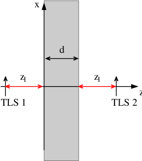
Figure 1: Sketch of the considered configuration.

The paper is organized as follows: In Sec. II we introduce the model and the general expressions needed to determine the concurrence function of two coupled TLS in the presence of a plasmonic environment which is described by the Green’s function given in Sec. III. In Sec. IV we compare the degree of entanglement between the TLS separated which can be achieved with a thin silver film with that of mulilayer hyperbolic meta-material. The conclusions of our study are given in Sec. V.

II Calculation of entanglement measure

The quantum entanglement arises from the radiative coupling between the two dipoles. Initially the atom A is excited and the atom B is in ground state. Thus to start with there is no entanglement between A and B atoms. When the atom A emits photon then this photon can be absorbed by the atom B leading to its excitation. This process can go on. Thus the quantum entanglement is produced by the dynamical evolution of the system of atoms. The dynamical evolution is most conveniently described in the master equation framework. The master equation is obtained by eliminating the radiative degrees of freedom and depends on the plasmonic or hyperbolic environment in which the atoms are located Agarwal1975 ; AgarwalBook . The density matrix of the two atoms is given by the environment dependent master equation ($i,j=1,2$)

$$\begin{split}\frac{\partial\rho}{\partial t}&=-{\rm i}\omega_{0}\sum_{j}[S_{j}^{z},\rho]-{\rm i}\sum_{i,j}\Omega_{ij}[S_{i}^{+}S_{j}^{-},\rho]\\ &\quad-\sum_{i,j}\gamma_{ij}[S_{i}^{+}S_{j}^{-}\rho-2S_{j}^{-}\rho S_{i}^{+}+\rho S_{i}^{+}S_{j}^{-}]\end{split}$$ (1)

where $\omega_{0}$ is the transition frequency of the two TLS, $S^{+}_{j}=|e_{j}\rangle\langle g_{j}|$ and $S^{-}_{j}=|g_{j}\rangle\langle e_{j}|$ are the atomic ladder operators and $S_{j}^{z}=\frac{1}{2}(|e_{j}\rangle\langle e_{j}|-|g_{j}\rangle\langle g_{j}|)$. The coupling of the two TLS via its environment which functions as a reservoir is described by

$$\gamma_{ij} :=\frac{1}{\epsilon_{0}}{\rm Im}\biggl{(}\frac{\omega_{0}^{2}}{c^{2}}\frac{1}{\hbar}\mathbf{p}_{i}\cdot\mathds{G}(\mathbf{r}_{i},\mathbf{r}_{j},\omega_{0})\cdot\mathbf{p}_{j}^{*}\biggr{)},$$ (2)

$$\Omega_{ij} :=-\frac{1}{\epsilon_{0}}{\rm Re}\biggl{(}\frac{\omega_{0}^{2}}{c^{2}}\frac{1}{\hbar}\mathbf{p}_{i}\cdot\mathds{G}(\mathbf{r}_{i},\mathbf{r}_{j},\omega_{0})\cdot\mathbf{p}_{j}^{*}\biggr{)}$$ (3)

introducing the dyadic Green’s function $\mathds{G}$ which determines the entire dynamics of our system. Typically, it can be written as a sum $\mathds{G}=\mathds{G}^{(0)}+\mathds{G}^{(s)}$ of the vacuum and a scattering part which takes the presence of the plasmonic or hyperbolic environment into account. Here, $\gamma_{11}$, $\gamma_{22}$ and $\Omega_{11}$, $\Omega_{22}$ are the single atom emission rates and level shifts of TLS 1 and 2 in the presence of the plasmonic environment, whereas $\gamma_{12},\gamma_{21},\Omega_{21}$ and $\Omega_{12}$ are the corresponding collective damping rates and level shifts. By writing the dipole moment of the two TLS as

$$\mathbf{p}_{i}:=p\mathbf{e}_{i},$$ (4)

where $\mathbf{e}_{i}$ is the general complex valued unit vector pointing in the direction of the dipole moment of TLS $i$, and introducing the free space emission rate of a single TLS AgarwalBook

$$\gamma_{0}:=\frac{2|p|^{2}\omega_{0}^{3}}{3c^{3}\hbar}\frac{1}{4\pi\epsilon_{0}}$$ (5)

we can express $\gamma_{ij}$ and $\Omega_{ij}$ as

$$\gamma_{ij} :=6\pi\gamma_{0}\frac{c}{\omega_{0}}{\rm Im}\biggl{(}\mathbf{e}_{i}\cdot\mathds{G}(\mathbf{r}_{i},\mathbf{r}_{j},\omega_{0})\cdot\mathbf{e}_{j}^{*}\biggr{)},$$ (6)

$$\Omega_{ij} :=-6\pi\gamma_{0}\frac{c}{\omega_{0}}{\rm Re}\biggl{(}\mathbf{e}_{i}\cdot\mathds{G}(\mathbf{r}_{i},\mathbf{r}_{j},\omega_{0})\cdot\mathbf{e}_{j}^{*}\biggr{)}.$$ (7)

If we consider a symmetric configuration as for example depicted in Fig. 1, we further have

$$\gamma_{12}=\gamma_{21}=:\gamma_{\rm c},$$ (8)

$$\gamma_{11}=\gamma_{22}=:\gamma_{\rm s},$$ (9)

$$\Omega_{12}=\Omega_{21}=:\Omega_{\rm c},$$ (10)

$$\Omega_{11}=\Omega_{22}=:\Omega_{\rm s}$$ (11)

where the indices stand for ’single’ and ’collective’. In this case we find the dynamical equations

$$\dot{\rho}_{ee} =-4\gamma_{\rm s}\rho_{ee},$$ (12)

$$\dot{\rho}_{eg} =-2\rho_{eg}[\gamma_{\rm s}+{\rm i}(\omega_{0}+\Omega_{\rm s})],$$ (13)

$$\dot{\rho}_{ss} =-2(\rho_{ss}-\rho_{ee})(\gamma_{\rm s}+\gamma_{\rm c}),$$ (14)

$$\dot{\rho}_{aa} =-2(\rho_{aa}-\rho_{ee})(\gamma_{\rm s}-\gamma_{\rm c}),$$ (15)

$$\dot{\rho}_{as} =-2\rho_{as}(\gamma_{\rm s}-{\rm i}\Omega_{\rm c})$$ (16)

for the states $|e\rangle=|e_{1}e_{2}\rangle$, $|g\rangle=|g_{1}g_{2}\rangle$, $|s\rangle=(|e_{1}g_{2}\rangle+|g_{1}e_{2}\rangle)/\sqrt{2}$ and $|a\rangle=(|e_{1}g_{2}\rangle-|g_{1}e_{2}\rangle)/\sqrt{2}$. These equations correspond to Eqs. (15.27) in Ref. AgarwalBook . Accordingly, the solutions of the dynamical equations are

$$\rho_{ee}(t) =\rho_{ee}(0){\rm e}^{-4\gamma_{\rm s}t},$$ (17)

$$\rho_{eg}(t) =\rho_{eg}(0){\rm e}^{-2[\gamma_{\rm s}+{\rm i}(\omega_{0}-\Omega_{\rm s})]t},$$ (18)

$$\rho_{as}(t) =\rho_{as}(0){\rm e}^{-2(\gamma_{\rm s}-{\rm i}\Omega_{\rm c})t},$$ (19)

$$\rho_{aa}(t) =\rho_{aa}(0){\rm e}^{-2(\gamma_{\rm s}-\gamma_{\rm c})t}$$

$$\quad-\frac{\gamma_{\rm s}-\gamma_{\rm c}}{\gamma_{\rm s}+\gamma_{\rm c}}\rho_{ee}(0)\biggl{(}{\rm e}^{-4\gamma_{\rm s}t}-{\rm e}^{-2(\gamma_{\rm s}-\gamma_{\rm c})t}\biggr{)},$$ (20)

$$\rho_{ss}(t) =\rho_{ss}(0){\rm e}^{-2(\gamma_{\rm s}+\gamma_{\rm c})t}$$

$$\quad-\frac{\gamma_{\rm s}+\gamma_{\rm c}}{\gamma_{\rm s}-\gamma_{\rm c}}\rho_{ee}(0)\biggl{(}{\rm e}^{-4\gamma_{\rm s}t}-{\rm e}^{-2(\gamma_{\rm s}+\gamma_{\rm c})t}\biggr{)}.$$ (21)

From these equations the dynamics of the system of TLS coupled by an arbitrary environment can be studied. Here we are interested in the entanglement which is measured by the concurrence function $C(t)$ introduced by Wootters Wootters1998 . This function is defined by $C=\max(0,\sqrt{\lambda_{1}}-\sqrt{\lambda_{2}}-\sqrt{\lambda_{3}}-\sqrt{\lambda_{4}})$ where the $\lambda_{i}$ ($i=1,\ldots,4$) are the eigenvalues of the matrix $\rho\tilde{\rho}$; $\tilde{\rho}$ can be defined by means of the Pauli matrix $\sigma_{y}$ by $\tilde{\rho}=\sigma_{y}\otimes\sigma_{y}\rho^{*}\sigma_{y}\otimes\sigma_{y}$. The concurrence functions has values between $[0,1]$ giving $0$ for unentangled states and $1$ for maximally entangled states. When starting at $t=0$ with the initially unentangled state $|e_{1},g_{2}\rangle$ then the concurrence function $C(t)$ is given by TanasFicek2004 ; AgarwalBook

$$C(t)={\rm e}^{-2\gamma_{\rm s}t}\sqrt{\sinh^{2}(2\gamma_{\rm c}t)+\sin^{2}(2\Omega_{\rm c}t)}.$$ (22)

It can be seen that $C(t=0)=0$ as expected, but for times $t>0$ it can have values larger than zero which means that due to the coupling of the two TLS via the environment an entanglement of the states of the two TLS is produced.

III Dyadic Green’s function

The goal is now to study the entanglement measured by the concurrence function for the two TLS when they are coupled by a thin film as depicted in Fig. 1. To this end, it is necessary to determine $\gamma_{\rm c}$, $\gamma_{\rm s}$ and $\Omega_{\rm c}$ which means that we have to determine the corresponding Green’s function for that configuration. For an initially excited TLS at $\mathbf{r}_{1}=(0,0,z_{1})^{t}$ with $z_{1}<0$ and a second TLS which is initially in the ground state at $\mathbf{r}_{2}=(0,0,z_{2}=d+|z_{1}|)^{t}$ the Green’s function in Weyl’s representation is given by

$$\mathds{G}(\mathbf{r_{1},r_{2}})=\int\!\!\frac{{\rm d}^{2}\kappa}{(2\pi)^{2}}\,\mathds{G}(\boldsymbol{\kappa},z)$$ (23)

where $\boldsymbol{\kappa}=(k_{x},k_{y})^{t}$ and

$$\mathds{G}(\boldsymbol{\kappa},z)=\frac{{\rm i}{\rm e}^{{\rm i}k_{z,{\rm vac}}(d+2|z_{1}|)}}{2k_{z,{\rm vac}}}\sum_{i={\rm s},{\rm p}}t_{i}\mathbf{a}_{i}^{+}(k_{0})\otimes\mathbf{a}_{i}^{+}(k_{0})$$ (24)

introducing the vacuum wavevector in z-direction $k_{z,{\rm vac}}=\sqrt{k_{0}^{2}-\kappa^{2}}$ and $k_{0}=\omega_{0}/c$. Here $t_{\rm s}$ and $t_{\rm p}$ are the amplitude transmission coefficients and $\mathbf{a}_{{\rm s},{\rm p}}^{+}$ are the polarization vectors defined by

$$\mathbf{a}_{\rm s}^{+}(k_{0}) =\frac{1}{\kappa}\begin{pmatrix}k_{y}\\ -k_{x}\\ 0\end{pmatrix},$$ (25)

$$\mathbf{a}_{\rm p}^{+}(k_{0}) =\frac{1}{\kappa k_{0}}\begin{pmatrix}-k_{x}k_{z,{\rm vac}}\\ -k_{y}k_{z,{\rm vac}}\\ \kappa^{2}\end{pmatrix}.$$ (26)

From this expression we can determine $\gamma_{\rm c}$ and $\Omega_{\rm c}$. On the other hand, if we want to determine $\gamma_{\rm s}$ we have to determine the the Green’s function $\mathds{G}(\mathbf{r_{1},r_{1}})$ evaluated solely at the position of the TLS which is initially in the excited state. In this case, we have

$$\mathds{G}(\mathbf{r}_{1},\mathbf{r}_{1})=\int\!\!\frac{{\rm d}^{2}\kappa}{(2\pi)^{2}}\,\mathds{G}^{\rm single}(\boldsymbol{\kappa},z)$$ (27)

with

$$\begin{split}\mathds{G}^{\rm single}(\boldsymbol{\kappa},z_{1})&=\frac{{\rm i}}{2k_{z,{\rm vac}}}\sum_{i={\rm s},{\rm p}}\biggl{[}\mathbf{a}_{i}^{+}(k_{0})\otimes\mathbf{a}_{i}^{+}(k_{0})\\ &\quad+{\rm e}^{2{\rm i}k_{z,{\rm vac}}|z_{1}|}r_{i}\mathbf{a}_{i}^{+}(k_{0})\otimes\mathbf{a}_{i}^{-}(k_{0})\biggr{]},\end{split}$$ (28)

where $r_{\rm s}$ and $r_{\rm p}$ are the amplitude reflection coefficients.

In order to see how the entanglement is affected by a plasmonic structure like a simple metal film or a hyperbolic meta-material we only need the appropriate expressions for the transmission and reflection coefficients. These are well known and for a in general uni-axial material with the optical axis oriented along the surface normal the transmission and reflection coefficients are given by

$$t_{\rm s} =\frac{4k_{z,{\rm o}}k_{z,{\rm vac}}{\rm e}^{{\rm i}(k_{z,{\rm o}}-k_{z,{\rm vac}})d}}{(k_{z,{\rm o}}+k_{z,{\rm vac}})^{2}-(k_{z,{\rm o}}-k_{z,{\rm vac}})^{2}{\rm e}^{2{\rm i}k_{z,{\rm o}}d}}$$ (29)

$$t_{\rm p} =\frac{4\epsilon_{\parallel}k_{z,{\rm e}}k_{z,{\rm vac}}{\rm e}^{{\rm i}(k_{z,{\rm e}}-k_{z,{\rm vac}})d}}{(k_{z,{\rm e}}+\epsilon_{\parallel}k_{z,{\rm vac}})^{2}-(k_{z,{\rm e}}-\epsilon_{\parallel}k_{z,{\rm vac}})^{2}{\rm e}^{2{\rm i}k_{z,{\rm e}}d}},$$ (30)

and

$$r_{\rm s} =R_{\rm s}\frac{1-{\rm e}^{2{\rm i}k_{z,{\rm o}}d}}{1-R_{\rm s}^{2}{\rm e}^{2{\rm i}k_{z,{\rm o}}d}},$$ (31)

$$r_{\rm p} =R_{\rm p}\frac{1-{\rm e}^{2{\rm i}k_{z,{\rm e}}d}}{1-R_{\rm p}^{2}{\rm e}^{2{\rm i}k_{z,{\rm e}}d}},$$ (32)

where we have introduced the reflection coefficients of a single interface

$$R_{\rm s} =\frac{k_{z,{\rm vac}}-k_{z,{\rm o}}}{k_{z,{\rm vac}}+k_{z,{\rm o}}},$$ (33)

$$R_{\rm p} =\frac{k_{z,{\rm vac}}\epsilon_{\perp}-k_{z,{\rm e}}}{k_{z,{\rm vac}}\epsilon_{\perp}+k_{z,{\rm e}}}$$ (34)

and the z components of the wavevector for the ordinary and extraordinary modes

$$k_{z,{\rm o}} =\sqrt{k_{0}^{2}\epsilon_{\perp}-\kappa^{2}},$$ (35)

$$k_{z,{\rm e}} =\sqrt{k_{0}^{2}\epsilon_{\perp}-\kappa^{2}\frac{\epsilon_{\perp}}{\epsilon_{\parallel}}}.$$ (36)

The permittivities $\epsilon_{\perp}$ and $\epsilon_{\parallel}$ are the permittivities perpendicular and parallel to the optical axis which is here the z axis, i.e. the optical axis is along the surface normal.

IV Metal vs HMM films

In the following we will consider a single silver film described by the Drude model

$$\epsilon_{\rm Ag}=\epsilon_{\parallel}=\epsilon_{\perp}=\epsilon_{\infty}-\frac{\omega_{\rm p}^{2}}{\omega(\omega+{\rm i}\tau^{-1})}.$$ (37)

The parameters from ChristyJohnson ; Soennichsen are $\epsilon_{\infty}=3.7$, $\omega_{\rm p}=1.4\cdot 10^{16}\,{\rm rad}/{\rm s}$,$\tau=4\cdot 10^{-14}\,{\rm s}$. As in Ref. BiehsEtAl2016 we use a much smaller relaxation time of $\tau=0.45\cdot 10^{-14}\,{\rm s}$ which accounts for the increased collission frequency found in thin metal films LangEtAl2013 . The surface plasmon resonance wavelength is in this case given by $\lambda_{\rm SP}=291\,{\rm nm}$ and the ENZ wavelength is $\lambda_{\rm ENZ}=259\,{\rm nm}$.

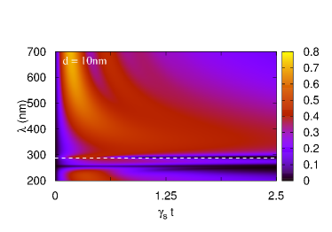
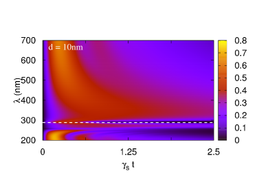
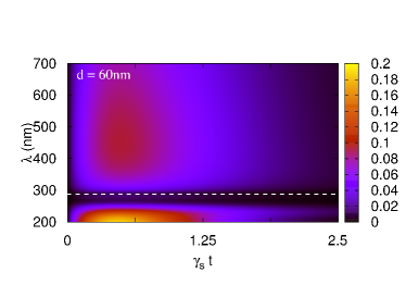
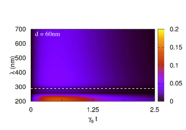
Figure 2: Concurrence function $C(t)$ for two TLS separated by a silver film of thicknesses $d=10\,{\rm nm}$ and $60\,{\rm nm}$. Left column is for x-orientation of the dipole moments and right column for the z-orientation. The dashed horizontal line marks the surface plasmon wavelength $\lambda_{\rm SP}=291\,{\rm nm}$.

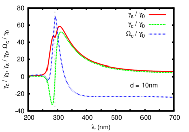
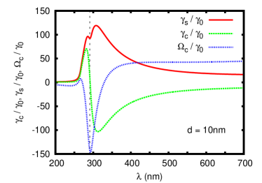
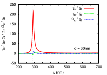
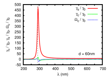
Figure 3: $\gamma_{\rm c}$, $\gamma_{\rm s}$ and $\Omega_{\rm c}$ for two TLS separated by a silver film of thicknesses $d=10\,{\rm nm}$ and $60\,{\rm nm}$ normalized to the free space emission rate $\gamma_{0}$. Left column is for x-orientation of the dipole moments and right column for the z-orientation. The dashed vertical line marks the surface plasmon wavelength $\lambda_{\rm SP}=291\,{\rm nm}$.

In Fig. 2 we show some examples for the concurrence function $C(t)$ for silver films of different thickness. Throughout the paper we choose $z_{1}=10\,{\rm nm}$. It can be seen that for very thin films with thickness $d=10\,{\rm nm}$ one can find a relatively large entanglement for $\lambda>\lambda_{\rm SP}$ of the two TLS due to the coupling via the coupled surface plasmons inside the metal film. On the other hand for thicker films with $d=60\,{\rm nm}$ the entanglement for $\lambda>\lambda_{\rm SP}$ becomes already very small and for $d=120\,{\rm nm}$ it is practically not existing. To get more inside why this happens we have plotted $\gamma_{\rm c}$, $\gamma_{\rm s}$ and $\Omega_{\rm c}$ in Fig. 3. As is clear from the expression for the concurrence function in Eq. (22) for $|\gamma_{\rm c}|t\gg 1$ or $\Omega_{\rm c}t\ll 1$ we have

$$C(t)\approx\frac{1}{2}{\rm e}^{2(|\gamma_{\rm c}|-\gamma_{\rm s})t}.$$ (38)

Obviously, in this limit the concurrence can only have a maximum value of 0.5 and there can only be a noticable entanglement if the collective damping rate $|\gamma_{\rm c}|$ is on the same order as the single-atom emission rate $\gamma_{\rm s}$. Since the energy transmission rate is proportional to $|\mathds{G}_{xx/zz}(\mathbf{r_{1},r_{2}})|^{2}=\gamma_{\rm c}^{2}+\Omega_{\rm c}^{2}$ this means that we can find a noticable entanglement if loosely speaking the ’energy transmission rate’ $|\gamma_{\rm c}|$ is on the same order of magnitude as the single-atom spontaneous emission rate $\gamma_{\rm s}$ of the initially excited TLS.

From Fig. 3 it becomes apparent that the spontaneous emimssion rate $\gamma_{\rm s}$ is very large around $\lambda_{\rm SP}$ as expected. Recently such changes in the spontaneous emission have also been studied for three-level systems on meta-surfaces and hyperbolic materials JhaEtAl2015 ; SunJiang2016 . In particular, the effect of the coupling of the surface plasmons in the thin silver film $d=10\,{\rm nm}$ can be nicely seen. The energy transmission rate is also very large for wavelengths around $\lambda_{\rm SP}$ as expected, but it drops rapidely when the film thickness is increased. This is so because the coupling between the surface plasmons on both interfaces becomes very small when $d$ is increased due to the evanescent nature of the surface plasmon polariton modes. This leads to a less efficient coupling of both TLS and therefore to very small entanglement for thicker metal films. Note, that at the ENZ wavelength of 259nm there is no significant effect of increased entanglement. The relatively large entanglement which can be seen in Fig. 2 for thick films is in the transparency region of the silver film for $\lambda<259\,{\rm nm}$.

In order to contrast the results obtained for metal films, we consider as a second structure a multilayer hyperbolic meta-material of alternating Ag and TiO₂ layers. The effective permittivities are for this structure given by

$$\epsilon_{\perp} =f\epsilon_{\rm Ag}+(1-f)\epsilon_{{\rm TiO}_{2}},$$ (39)

$$\epsilon_{\parallel} =\frac{\epsilon_{\rm Ag}\epsilon_{{\rm TiO}_{2}}}{f\epsilon_{{\rm TiO}_{2}}+(1-f)\epsilon_{\rm Ag}},$$ (40)

where $f$ is the filling fraction of silver and $\epsilon_{\rm Ag}$/$\epsilon_{{\rm TiO}_{2}}$ are the permittivites of the both constitutents of the multilayer structure. For silver we use the Drude model in Eq. (37). TiO₂ is transparent in the visible regime. It’s permittivity $\epsilon_{{\rm TiO}_{2}}$ is nearly constant in that regime and can be well described by the formula Devore1951

$$\epsilon_{{\rm TiO}_{2}}=5.913+\frac{0.2441}{\lambda^{2}-0.0803}.$$ (41)

As shown in Ref. BiehsEtAl2016 when choosing $f=0.35$ this multilayer structure has a type I hyperbolic band [${\rm Re}(\epsilon_{\parallel})<0$ and ${\rm Re}(\epsilon_{\perp})>0$] at wavelengths below the epsilon-near-pole wavelength $\lambda_{\rm ENP}=395\,{\rm nm}$ and a type II hyperbolic band [${\rm Re}(\epsilon_{\parallel})>0$ and ${\rm Re}(\epsilon_{\perp})<0$] above the epsilon-near-zero wavelength $\lambda_{\rm ENZ}=551\,{\rm nm}$. For $\lambda_{\rm ENP}<\lambda<\lambda_{\rm ENZ}$ the multilayer structure behaves like a normal uni-axial dielectric [${\rm Re}(\epsilon_{\parallel})>0$ and ${\rm Re}(\epsilon_{\perp})>0$].

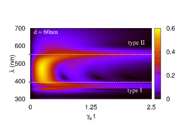
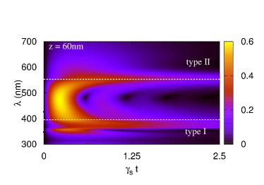
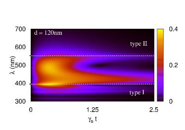
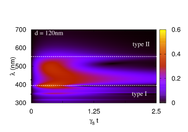
Figure 4: Concurrence function $C(t)$ for two TLS separated by a HMM film of thicknesses $d=60\,{\rm nm}$ and $120\,{\rm nm}$. Left column is for x-orientation of the dipole moments and right column for the z-orientation. The horizontal dashed lines mark the ENP and ENZ wavelengths $\lambda_{\rm ENP}=395\,{\rm nm}$ and $\lambda_{\rm ENZ}=551\,{\rm nm}$.

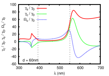
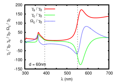
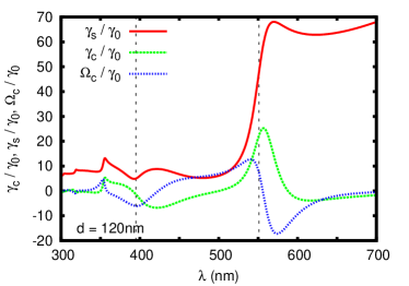
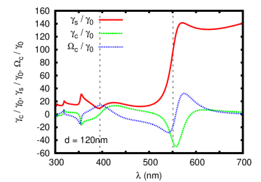
Figure 5: $\gamma_{\rm c}$, $\gamma_{\rm s}$ and $\Omega_{\rm c}$ for two TLS separated by a HMM film of thicknesses $d=60\,{\rm nm}$ and $120\,{\rm nm}$ normalized to the free space emission rate $\gamma_{0}$. Left column is for x-orientation of the dipole moments and right column for the z-orientation. The vertical dashed lines mark the ENP and ENZ wavelengths $\lambda_{\rm ENP}=395\,{\rm nm}$ and $\lambda_{\rm ENZ}=551\,{\rm nm}$.

In Fig. 4 we show the concurrence function for the HMM as a function of time and wavelength for $d=60\,{\rm nm}$ and $120\,{\rm nm}$. It can be seen that for $d=60\,{\rm nm}$ the entanglement is especially large at the ENZ and ENP wavelength. For $d=120\,{\rm}$ we have still a relatively large entanglement especially close to the ENZ wavelength and in the normal dielectric region with $\lambda_{\rm ENP}<\lambda<\lambda_{\rm ENZ}$. As can be seen in Fig. 5 this is in agreement with the large transmission at the ENZ wavelength which has been studied in very much detail in Ref. BiehsEtAl2016 . The difference to the silver film is that here we have propagating modes inside the hyperbolic material with large wavevectors allowing a strong coupling between the two TLS even for relatively thick films. The main limiting factor for this strong coupling is the damping of these propagating modes inside the hyperbolic materials. Apart from the fact that we can have large entanglement for relatively thick films hyperbolic materials have the advantage that the position of the ENP and ENZ wavelength can be engineered by the combination of different materials and by changing the filling fraction of the metal part of the structure so that the wavelength for which a strong coupling is needed can be adapted at will.

V Conclusion

To summarize, we have studied the entanglement of two TLS separated by a thin film using the master-equation approach and the concurrence function as entanglement measure. We have compared the entanglement as function of the film thickness of the intermediate layer for a silver film and a multilayer Ag/TiO₂ hyperbolic meta-material. Our main finding is summarized in Fig. 6 where the concurrence function is plotted for the silver film and the hyperbolic material close to the ENZ wavelength at 550nm for different film thicknesses. At this wavelength the single-atom emission rates and the energy transmission rates for the TLS in presence of the hyperbolic material are very large compared to the vacuum value. By changing the filling fraction of the silver layers in the Ag/TiO₂ hyperbolic meta-material one can shift this important frequency. It can be seen in Fig. 6 that for the hyperbolic material one can find the same entanglement as for the metallic film but for twice as thick layers. At the ENZ wavelength of the metallic film we find in most cases a relatively small entanglement as is shown in Fig. 6 so that for operation at the ENZ wavelengths hyperbolic metamaterial are much more advantageous than metal films. We believe that by optimizing the vertical and horizontal positions of the TLS and by optimizing the multilayer layout one can achieve substantial entanglement even for thicker films.

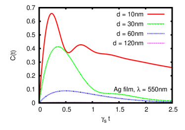
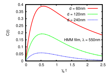
Figure 6: Concurrence function for two TLS separated by an Ag and a HMM film with x-oriented dipole moments for different thicknesses evaluated at the ENZ wavelength $\lambda=550\,{\rm nm}$ of the HMM.

Appendix

Appendix A Derivation of $\mathds{G}_{xx}$ and $\mathds{G}_{zz}$

If the dipole moments of the TLS are oriented both in $z$ or $x$ directions. In this case the above expressions can be further simplified.

A.1 Dipoles in z-direction

If the dipole moments are oriented in z-direction we find

$$[\mathbf{a}_{\rm s}^{\pm}(k_{0})\otimes\mathbf{a}_{\rm s}^{\pm}(k_{0})]_{zz} =0,$$ (42)

$$[\mathbf{a}_{\rm p}^{\pm}(k_{0})\otimes\mathbf{a}_{\rm p}^{\pm}(k_{0})]_{zz} =\frac{\kappa^{2}}{k_{0}^{2}}$$ (43)

and therefore

$$\mathds{G}_{zz}(\mathbf{r}_{1},\mathbf{r}_{2})=\int\frac{{\rm d}\kappa}{2\pi}\,\kappa\frac{{\rm i}{\rm e}^{{\rm i}k_{z,{\rm vac}}(d+2|z_{1}|)}}{2k_{z,{\rm vac}}}t_{\rm p}\frac{\kappa^{2}}{k_{0}^{2}}$$ (44)

and

$$\mathds{G}_{zz}^{\rm single}(\mathbf{r}_{1},\mathbf{r}_{1})=\int\frac{{\rm d}\kappa}{2\pi}\,\kappa\frac{{\rm i}}{2k_{z,{\rm vac}}}\frac{\kappa^{2}}{k_{0}^{2}}\biggl{(}1+r_{\rm p}{\rm e}^{2{\rm i}k_{z,{\rm vac}}|z_{1}|}\biggr{)}.$$ (45)

From this expression we can retrieve the results for the case where the TLS are only coupled by vacuum by setting $t_{\rm p}=1$ and $r_{\rm p}=0$ so that

$$\mathds{G}_{zz}^{\rm vac}(\mathbf{r}_{1},\mathbf{r}_{2})=\int\frac{{\rm d}\kappa}{2\pi}\,\kappa\frac{{\rm i}{\rm e}^{{\rm i}k_{z,{\rm vac}}(d+2|z_{1}|)}}{2k_{z,{\rm vac}}}\frac{\kappa^{2}}{k_{0}^{2}}$$ (46)

and

$$\mathds{G}_{zz}^{\rm single,vac}(\mathbf{r}_{1},\mathbf{r}_{1})=\int\frac{{\rm d}\kappa}{2\pi}\,\kappa\frac{{\rm i}}{2k_{z,{\rm vac}}}\frac{\kappa^{2}}{k_{0}^{2}}.$$ (47)

The emission rate for the single atom in vacuum is in this case

$$\gamma_{\rm s}^{\rm vac}=\frac{6\pi\gamma_{0}}{k_{0}}{\rm Im}(\mathds{G}_{zz})=\frac{6\pi\gamma_{0}}{k_{0}}\frac{1}{4\pi}k_{0}\frac{2}{3}=\gamma_{0}.$$ (48)

A.2 Dipoles in x-direction

If the dipole moments of the TLS are oriented in x-direction we find

$$[\mathbf{a}_{\rm s}^{\pm}(k_{0})\otimes\mathbf{a}_{\rm s}^{\pm}(k_{0})]_{xx} =\frac{k_{y}^{2}}{\kappa^{2}},$$ (49)

$$[\mathbf{a}_{\rm p}^{\pm}(k_{0})\otimes\mathbf{a}_{\rm p}^{\pm}(k_{0})]_{xx} =\frac{k_{x}^{2}k_{z,{\rm vac}}^{2}}{\kappa^{2}k_{0}^{2}}.$$ (50)

Introducing polar coordinates for $\boldsymbol{\kappa}=\kappa(\cos\theta,\sin\theta)^{t}$ we find therefore

$$\mathds{G}_{xx}(\mathbf{r}_{1},\mathbf{r}_{2})=\int\frac{{\rm d}\kappa}{2\pi}\,\kappa\frac{{\rm i}{\rm e}^{{\rm i}k_{z,{\rm vac}}(d+2|z_{1}|)}}{2k_{z,{\rm vac}}}\frac{1}{2}\biggl{(}t_{\rm s}+t_{\rm p}\frac{k_{z,{\rm vac}}^{2}}{k_{0}^{2}}\biggr{)}$$ (51)

and

$$\begin{split}\mathds{G}_{xx}^{\rm single}(\mathbf{r}_{1},\mathbf{r}_{1})&=\int\frac{{\rm d}\kappa}{2\pi}\,\kappa\frac{{\rm i}}{2k_{z,{\rm vac}}}\biggl{[}\frac{k_{0}^{2}+k_{z,{\rm vac}}^{2}}{2k_{0}^{2}}\\ &\qquad+{\rm e}^{2{\rm i}k_{z,{\rm vac}}|z_{1}|}\frac{1}{2}\biggl{(}r_{\rm s}-r_{\rm p}\frac{k_{z,{\rm vac}}^{2}}{k_{0}^{2}}\biggr{)}\biggr{]}.\end{split}$$ (52)

Again we can retrieve the relations for the case where both TLS are coupled by vacuum by setting $t_{\rm p}=1$ and $r_{\rm p}=0$ so that

$$\mathds{G}_{xx}^{\rm vac}(\mathbf{r}_{1},\mathbf{r}_{2})=\int\frac{{\rm d}\kappa}{2\pi}\,\kappa\frac{{\rm i}{\rm e}^{{\rm i}k_{z,{\rm vac}}(d+2|z_{1}|)}}{2k_{z,{\rm vac}}}\frac{1}{2}\biggl{(}1+\frac{k_{z,{\rm vac}}^{2}}{k_{0}^{2}}\biggr{)}$$ (53)

and

$$\mathds{G}_{xx}^{\rm single,vac}(\mathbf{r}_{1},\mathbf{r}_{1})=\int\frac{{\rm d}\kappa}{2\pi}\,\kappa\frac{{\rm i}}{2k_{z,{\rm vac}}}\frac{k_{0}^{2}+k_{z,{\rm vac}}^{2}}{2k_{0}^{2}}$$ (54)

The emission rate for the single atom in vacuum is in this case again

$$\gamma_{\rm s}^{\rm vac}=\frac{6\pi\gamma_{0}}{k_{0}}{\rm Im}(\mathds{G}_{xx})=\frac{6\pi\gamma_{0}}{k_{0}}\frac{1}{4\pi}k_{0}\frac{2}{3}=\gamma_{0}.$$ (55)

References

• (1) P. W. Milonni, The Quantum Vacuum, (Academic Press, 1994).
• (2) A. I. Volokitin and B. N. J. Persson, “Near-field radiative heat transfer and noncontact friction,” Rev. Mod. Phys. 79, 1291–1329 (2007).
• (3) T. Förster,“Zwischenmolekulare Energiewanderung und Fluoreszenz,” Ann. Phys. 437, 55–75 (1948).
• (4) H. T. Dung, L. Knöll, and D.-G. Welsch, “Intermolecular energy transfer in the presence of dispersing and absorbing media,” Phys. Rev. A 65, 043813 (2002).
• (5) S.-A. Biehs and G. S. Agarwal, “Dynamical quantum theory of heat transfer between plasmonic nanosystems,” J. Opt. Soc. Am. B 30, 700 (2013).
• (6) M. A. Nielsen and I. L. Chuang, Quantum Computation and Quantum Information, (Cambridge University Press, Cambridge,2000).
• (7) I. Bouchoule and K. Molmer, “Spin squeezing of atoms by the dipole interaction in virtually excited Rydberg states,” Phys. Rev. A 65, 041803 (2002).
• (8) L. Isenhower, E. Urban, X. L. Zhang, A. T. Gill, T. Henage, T. A. Johnson, T. G. Walker, and M. Saffman, “Demonstration of a Neutral Atom Controlled-NOT Quantum Gate,” Phys. Rev. Lett. 104, 010503 (2010).
• (9) G. V. Varada and G. S. Agarwal, “Two-photon resonance induced by the dipole-dipole interaction,” Phys. Rev. A 45, 6721 (1992).
• (10) H. R. Haakh and D. Martín-Cano, “Squeezed light from entangled nonidentical emitters via nanophotonic environments,” ACS Photonics 2, 1686–1691 (2015).
• (11) C. Hettich, C. Schmitt, J. Zitzmann, S. Kühn, I. Gerhardt and V. Sandoghdar, “Nanometer Resolution and Coherent Optical Dipole Coupling of Two Individual Molecules,” Science 298, 385 (2002).
• (12) M. Saffman, T. G. Walker, T. G. and K. Molmer, “Quantum information with Rydberg atoms,” Rev. Mod. Phys. 82, 2313 (2010).
• (13) J. Gillet, G. S. Agarwal and T. Bastin, “Tunable entanglement, antibunching, and saturation effects in dipole blockade,” Phys. Rev. A 81, 013837 (2010).
• (14) K. A. Velizhanin and T. V. Shahbazayan, “Long-range plasmon-assisted energy transfer over doped graphene,” Phys. Rev. B 86, 245432 (2012).
• (15) G. S. Agarwal and S.-A. Biehs, “Highly nonparaxial spin Hall effect and its enhancement by plasmonic structures,” Opt. Lett. 38, 4421 (2013).
• (16) V. D. Karanikolas, C. A. Marocico, and A. L. Bradley, “Tunable and long-range energy transfer efficiency through a graphene nanodisk,” Phys. Rev. B 93, 035426 (2016).
• (17) S.-A. Biehs and G. S. Agarwal, “Large enhancement of Förster resonance energy transfer on graphene platforms,” Appl. Phys. Lett. 103, 243112 (2013).
• (18) A. Poudel, X. Chen, and M. A. Ratner, “Enhancement of Resonant Energy Transfer Due to an Evanescent Wave from the Metal,” J. Phys. Chem. Lett. 7, 955–960 (2016).
• (19) J. Li, S. K. Cushing, F. Meng, T. R. Senty, A. D. Bristow, and N. Wu, “Plasmon-induced resonance energy transfer for solar energy conversion,” Nat. Phot. 9, 601–607 (2015).
• (20) D. Martin-Cano, L. Martín-Moreno, F.J. García-Vidal, and E. Moreno, “Resonance Energy Transfer and Superradiance Mediated by Plasmonic Nanowaveguides,” Nano Lett. 10, 3129(2010).
• (21) D. Bouchet, D. Cao, R. Carminati, Y. De Wilde, and V. Krachmalnicoff, “Long-Range Plasmon-Assisted Energy Transfer between Fluorescent Emitters,” Phys. Rev. Lett. 116, 037401 (2016).
• (22) P. Andrew and W. L. Barnes, “Energy Transfer Across a Metal Film Mediated by Surface Plasmon Polaritons,” Science 306, 1002–1005 (2004).
• (23) S.-A. Biehs, V. M. Menon, and G. S. Agarwal, “Long-range dipole-dipole interaction and anomalous Förster energy transfer across a hyperbolic metamaterial,” Phys. Rev. B 93, 245439 (2016).
• (24) C. L. Cortes and Z. Jacob, “Super-Coulombic atom-atom interactions in hyperbolic media,” Nat. Comm. 8, 14144 (2017).
• (25) I. Liberal and N. Engheta, “Nonradiating and radiating modes excited by quantum emitters in open epsilon-near-zero cavities”, Science Advances 2, e1600987 (2016).
• (26) M. Z. Alam, I. De Leon, R. W. Boyd, “Large optical nonlinearity of indium tin oxide in its epsilon-near-zero region”. Science 352, 795 (2016).
• (27) M. Silverinha and N. Engheta, “Tunneling of Electromagnetic Energy through Subwavelength Channels and Bends using $\epsilon$-Near-Zero Materials”, Phys. Rev. Lett. 97, 157403 (2006).
• (28) A. Alu, M. Silverinha, A. Salandrino, and N. Engheta, “Epsilon-near-zero metamaterials and electromagnetic sources: Tailoring the radiation phase pattern”, Phys. Rev. B 75, 155410 (2007).
• (29) S. Lang, M. Tschikin, S.-A. Biehs, A. Yu. Petrov, and M. Eich, “Large penetration depth of near-field heat flux in hyperbolic media,” Appl. Phys. Lett. 104, 121903 (2014).
• (30) J. Liu and E. E. Narimanov, “Thermal hyperconductivity: Radiative energy transport in hyperbolic media” Phys. Rev. B 91, 041403(R) (2015).
• (31) S.-A. Biehs, S. Lang, A. Yu. Petrov, M. Eich, and P. Ben-Abdallah, “Black-body theory for hyperbolic materials,” Phys. Rev. Lett. 115, 174301 (2015).
• (32) R. Messina, P. Ben-Abdallah, B. Guizal, M. Antezza, S.-A. Biehs, “Hyperbolic waveguide for long-distance transport of near-field heat flux,” Phys. Rev. B 94, 104301 (2016).
• (33) G. S. Agarwal, “Quantum electrodynamics in the presence of dielectrics and conductors. IV. General theory for spontaneous emission in finite geometries,”, Phys. Rev. A 12, 1475 (1975).
• (34) G. S. Agarwal, Quantum Optics, (Cambridge University Press, Cambridge, 2012).
• (35) W. K. Wootters, “Entanglement of Formation of an Arbitrary State of Two Qubits,” Phys. Rev. Lett. 80, 2245 (1998).
• (36) R. Tanaś and Z. Ficek, “Entangling two atoms via spontaneous emission,” J. Opt. B: Quantum Semiclass. Opt. 6, S90 (2004).
• (37) C. Sönnichsen, Plasmons in metal nanostructures, PhD thesis (2001).
• (38) P. B. Johnson and R. W. Christy, “Optical Constants of the Noble Metals,” Phys. Rev. B 6, 4370 (1972).
• (39) S. Lang, H. S. Lee, A. Yu. Petrov, M. Störmer, M. Ritter, and M. Eich, “Gold-silicon metamaterial with hyperbolic transition in near infrared,” Appl. Phys. Lett. 103, 021905 (2013).
• (40) P. K. Jha, X. Ni, C. Wu, Y. Wang, and X. Zhang, “Metasurface-Enabled Remote Quantum Interference, ” Phys. Rev. Lett. 115, 025501 (2015).
• (41) L. Sun and C. Jiang, “Quantum interference in a single anisotropic quantum dot near hyperbolic metamaterials”, Opt. Expr. 24, 258788 (2016).
• (42) J. R. Devore, “Refractive Indices of Rutile and Sphalerite,” J. Opt. Soc. Am. 41, 416–419 (1951).