Position determination and strong field parallax effects for photon emitters in the Schwarzschild spacetime

Abstract

Position determination of photon emitters and associated strong field parallax effects are investigated using relativistic optics when the photon orbits are confined to the equatorial plane of the Schwarzschild spacetime. We assume the emitter is at a fixed space position and the receiver moves along a circular geodesic orbit. This study requires solving the inverse problem of determining the (spatial) intersection point of two null geodesic initial data problems, serving as a simplified model for applications in relativistic astrometry as well as in radar and satellite communications.

1 Introduction

The optics of photon motion in the Schwarzschild spacetime is well known and standardized in many textbooks in terms of an analytic representation using elliptic functions (see e.g., Refs. Darwin:1959 ; Misner:1974qy ; Luminet:1979 ; Chandrasekhar:1985kt and the more recent reviews Cadez:2005 ; Munoz:2014 ), but its application to parallax effects and stellar position determination has not received much attention. The present article aims to accomplish this goal in a fully relativistic strong field context, while simultaneously showing how these calculations approach the more familiar ones of nearly flat spacetime in the weak field regime Arifov:1969 ; Semerak:2014kra . Of course the approximation methods of space astrometry are sufficient to consider parallax effects of stars seen from Earth or from space using the Gaia satellite project gaia or future satellite measurements like LISA LISA . However, it is interesting in principle to investigate how one can handle them in strong gravitational fields with nontrivial curved spacetime optics.

To avoid excessive complication we consider here the special case of photons emitted from a point in the same plane as an observer moving in a stable circular orbit around a black hole or other compact object described by the Schwarzschild spacetime beyond some minimal radius. Then relatively simple but curved 2-dimensional spatial geometry can be used to model both the emitter, the receiver and photon orbits between them, a scenario which in turn can also be easily compared to the corresponding flat spacetime case.

We consider a stable timelike circular geodesic orbit $r=r_{0}\geq 6M$ in the equatorial plane $\theta=\pi/2$ of the Schwarzschild spacetime of mass $M$ receiving photons emitted from a point $P_{*}$ fixed in the spatial grid of the usual Boyer-Lindquist coordinates $(t,r,\theta,\phi)$ in that plane and study how to recover the emitter point coordinates $(r_{*},\phi_{*})$ from the angle of reception $\beta_{0}$ with respect to the azimuthal coordinate direction and the location $\phi_{0}$ on the receiving circle for two incoming such photons. The null geodesics in the Schwarzschild equatorial plane can be expressed giving the polar angle as a function of the radial coordinate using elliptic functions and parametrized by the conserved angular momentum along each photon trajectory. The latter in turn can be expressed in terms of the arrival angle $\beta_{0}$. One then has to (numerically) solve a pair of elliptic function relationships for the desired coordinates $(r_{*},\phi_{*})$ given two sets of values for $(\phi_{0},\beta_{0})$.

By using the orthonormal frame obtained by normalizing the coordinate frame vectors, corresponding to measurements by the static observers whose world lines are the time coordinate lines, stellar aberration effects due to the relative motion of the circularly orbiting observer are avoided, but can be calculated afterwards, see Appendix A. We start by setting up the geometry in the corresponding flat Minkowski spacetime using the same coordinate grid and will use this comparison later to consider the linearized corrections to the exact curved photon motion compared to the flat case.

2 The flat spacetime scenario

Let $(t,x,y,z)$ be inertial coordinates on flat Minkowski spacetime (signature $-+++$) with corresponding spherical spatial coordinates $(t,r,\theta,\phi)$, so that the line element reads $ds^{2}=-dt^{2}+dr^{2}+r^{2}(d\theta^{2}+\sin^{2}\theta\,d\phi^{2})$ and let ${n}=\partial_{t}$ be the 4-velocity of the corresponding inertial observers. The spatial spherical orthonormal frame is given by

$$e_{\hat{r}}=\partial_{r}\,,\quad e_{\hat{\theta}}=\frac{1}{r}\,\partial_{\theta}\,,\quad e_{\hat{\phi}}=\frac{1}{r}\,\partial_{\phi}\,.$$ (1)

Consider an accelerated (timelike) circular orbit in the equatorial plane $\theta=\pi/2$ of flat Minkowski spacetime in spherical coordinates $(t,r,\theta,\phi)$

$$t=t\,,\ r=r_{0}\,,\ \theta=\pi/2\,,\ \phi=\Omega\,t\,,\$$ (2)

with $\Omega>0$. An observer moving along this circular orbit has 4-velocity

$$U=\gamma(U,n)({n}+\nu(U,{n}))\,,\quad\nu(U,{n})=\nu(U,{n})^{\hat{\phi}}e_{\hat{\phi}}\,,\quad\nu(U,{n})^{\hat{\phi}}=\Omega\,r_{0}\,.$$ (3)

We will later choose $\Omega$ to be the coordinate frequency for the corresponding circular geodesic orbit in the Schwarzschild spacetime at this radius (given a fixed mass $M$).

Equatorial plane null geodesics representing photons emitted from a point $P_{*}$, chosen here to lie on the positive $x$ axis only for convenience in our diagrams, arrive at each point of the circular orbit via a straight line trajectory, shown in Fig. 1. The geodesic equations describing these orbits parametrized by an affine parameter $\lambda$ (so that $P^{\alpha}=dx^{\alpha}/d\lambda$), are given by

$$\frac{dt}{d\lambda} = E\,,$$

$$\frac{dr}{d\lambda} = \pm E\sqrt{1-\frac{\ell^{2}}{r^{2}}}\,,$$

$$\frac{d\phi}{d\lambda} = \frac{E\,\ell}{r^{2}}\,,$$ (4)

where the $\pm$ sign distinguishes the radially outgoing and ingoing directions. $E=E(P,n)$ is the conserved energy and $L_{z}\equiv E\ell$ is the conserved angular momentum allowing their 4-momentum to be expressed in the form

$$P = E({n}+\hat{\nu}(P,{n}))=E\left(\partial_{t}\pm\sqrt{1-\frac{\ell^{2}}{r^{2}}}\partial_{r}+\frac{\ell}{r^{2}}\partial_{\phi}\right)\,,$$ (5)

with unit spatial velocity

$$\hat{\nu}(P,{n})=\pm\sqrt{1-\frac{\ell^{2}}{r^{2}}}\,e_{\hat{r}}+\frac{\ell}{r}\,e_{\hat{\phi}}\equiv\sin\beta\,e_{\hat{r}}+\cos\beta\,e_{\hat{\phi}}\,,$$ (6)

defining the angle $\beta$ it makes with the azimuthal direction $e_{\hat{\phi}}$ in the clockwise direction as shown in Fig. 1, so that $\beta<0$ as $r$ decreases.

The 4-momentum $P$ of Eq. (5) referred to the rotating observer on the circular orbit (instead of the inertial observers of the coordinate grid) can be expressed as

$$P = E(P,U)(U+\hat{\nu}(P,U))\,,$$ (7)

with unit spatial velocity $\hat{\nu}(P,U)$ with respect to $U$. The two energies are related by

$$E(P,U) = \gamma(U,n)E(P,n)\left(1-\nu(U,{n})\cdot\hat{\nu}(P,{n})\right)$$ (8)

$$= \gamma(U,n)E(1-\Omega\,r_{0}\cos\beta)\,,$$

which describes the Doppler effect on the photon frequency if we set $E=\hbar\omega$, $E(P,U)=\hbar\omega(P,U)$. Eqs. (5), (7) may also be used to evaluate the angle $\beta_{U}$ of the incoming photon seen by the rotating observer due to aberration, a completely special relativistic effect discussed in detail in Appendix A.

Using the coordinate time $t=E\lambda$ as a new parameter along the photon orbits, the geodesic equations reduce to

$$\frac{dr}{dt} = \pm\sqrt{1-\frac{\ell^{2}}{r^{2}}}\,,\qquad\qquad\frac{d\phi}{dt}=\frac{\ell}{r^{2}}\,,$$ (9)

or introducing the reciprocal radius $u=1/r$ to compare with the Schwarzschild case below

$$\frac{dt}{du}=\mp\frac{1}{u^{2}\sqrt{1-\ell^{2}u^{2}}}\,,\quad\frac{d\phi}{du}=\mp\frac{\ell}{\sqrt{1-\ell^{2}u^{2}}}=\mp\frac{{\rm sgn}(\ell)}{\sqrt{\ell^{-2}-u^{2}}}\,.$$ (10)

The turning point $Q$ for the radial motion where this vanishes occurs at $r=|\ell|$, $\phi=\phi^{(0)}$, giving $|\ell|$ the interpretation as the impact parameter for this orbit (minimal radius), and requiring $r\geq|\ell|$. The time parameter measures the proper arclength along the photon trajectories, for which it is natural to choose the initial conditions at $t=t_{0}$ at the minimal radius $r|_{t=t_{0}}=|\ell|,\phi|_{t=t_{0}}=\phi^{(0)}$, splitting the solutions into two segments, along which the radius is either monotonically increasing or decreasing with time, and is an even function of the difference $t-t_{0}$ or $\phi-\phi^{(0)}$. The sign of $\ell$ introduces another sign factor into the rate of change of radius with respect to angle in Eq. (10). Let $\phi^{(1)}$ denote the angle where the photon orbit first intersects the circular orbit (at $P_{1}$) and $\phi^{(2)}$ the second such intersection point ($P_{2}$), symmetrically located with respect to $Q$ and related by $\phi^{(0)}=(\phi^{(1)}+\phi^{(2)})/2$. Note that $\phi^{(0)}$, $\phi^{(1)}$, $\phi^{(2)}$ all depend on $\ell$, even if not explicitly shown in the notation. Figs. 1,2 illustrate this situation.

Figure 1: The photon orbit in the $(r,\phi)$ plane from the point $P_{*}$ (chosen to have $\phi_{*}=0$) intersecting a circular orbit of radius $r_{0}$, shown for the case $\ell>0$ ($\ell<0$) above (below) the horizontal axis. The point $Q$ of closest approach to the origin has polar coordinates $(\ell,\phi^{(0)})$. For the part of the orbit from $P_{*}$ to $Q$, $r$ decreases to $\ell$ after which it increases. The counterclockwise angle $\beta$ of the incoming photon velocity with respect to the forward azimuthal direction is a negative acute angle decreasing to 0 when the photon orbit reaches $Q$ and then turns positive. The case $\ell<0$ corresponds to reflecting this diagram across the horizontal axis, so that the relative azimuthal direction is the supplement of the corresponding previous case, and $\beta$ is a negative obtuse angle decreasing to $-\pi$ at $Q$ and then taking values less than $-\pi$. One also sees that the difference angle $\chi=\phi-\phi^{(0)}=\beta<0$ for $\ell>0$ and $\chi=\pi+\beta>0$ for $\ell<0$.

Figure 2: The straight line photon orbit in the $(r,\phi)$ plane as in Fig. 1 connecting the point $P_{*}$ to $P_{1}$ and then $P_{2}$, shown with the angle of reception $\beta$ at $P_{1}$ on the circular orbit for $\ell>0$, and its complement for $\ell<0$. The radial motion negative sign is appropriate for the segment $P_{\ast}Q$ and the plus sign for $QP_{2}$.

From the geometry of Fig. 1, one can write down an arclength parametrized straight line solution to the photon orbit equations in the polar coordinates. If the photon orbit arrives at point $Q$ at $t=t_{0}$, since increments of $t$ measure arclength along the orbit, it is clear that the hypotenuse of the right triangle has length $|t-t_{0}|$, so

$$r(t)=\sqrt{\ell^{2}+(t-t_{0})^{2}}\,,\quad\tan(\phi-\phi^{(0)})=\frac{t-t_{0}}{\ell}\,.$$ (11)

Similarly, referring to the same Fig. 1, one can introduce a new angle $\chi=\phi-\phi^{(0)}$ along the photon orbit for which $\cos\chi=|\ell|/r=|\ell|u$ and so

$$r(\phi)=\frac{|\ell|}{\cos\chi}=\frac{|\ell|}{\cos(\phi-\phi^{(0)})}\,,$$ (12)

or equivalently

$$|\phi-\phi^{(0)}|=\arccos(|\ell|u)\,.$$ (13)

As follows from the geometry of Figs. 1 and 2, for $\ell>0$, $\chi<0$ increases along the photon orbit from $\chi_{*}=\phi_{*}-\phi^{(0)}<0$ to 0 at $\phi=\phi^{(0)}$ (decreasing $r$) and then goes positive (increasing $r$). For $\ell<0$, $\chi$ decreases from $\chi_{*}>0$ to 0 at $\phi=\phi^{(0)}$ (decreasing $r$) and then goes negative (increasing $r$). In both cases $|\chi_{*}|<\pi/2$.

On the other hand the orbital equations (10) directly suggest the change of variable $\cos\chi=|\ell|u$, so that $-\sin\chi\,d\chi=|\ell|du$, and then along the photon orbit the angular equation for $\ell>0$ reduces to ${d\phi}/{d\chi}=1$ as it should, while the time equation integrates to

$$t=t_{0}+\ell\tan\chi\,,$$ (14)

and hence

$$t=t_{0}\pm\frac{1}{u}\sqrt{1-\ell^{2}u^{2}}\,,$$ (15)

reproducing the radial solution (11).

To compare the present simple, flat spacetime discussion with the more complicated change of variable needed for the Schwarzschild case, we consider the roots $u_{1}=-{1}/{|\ell|}<0$ and $u_{2}={1}/{|\ell|}$ of the key quadratic expression appearing in the orbital equations

$$1-u^{2}\ell^{2}=-\ell^{2}(u-u_{1})(u-u_{2})\,,$$ (16)

which leads to the following change of variable using the new angle $\bar{\chi}$ supplementary to $\chi$, namely $\cos(\pi-\bar{\chi})=-\cos\bar{\chi}=|\ell|/r=|\ell|u=\cos\chi$ which is equivalent to

$$\sin\left(\frac{\bar{\chi}}{2}\right)=\sqrt{\frac{\bar{u}-\bar{u}_{1}}{\bar{u}_{2}-\bar{u}_{1}}}\,,$$ (17)

or

$$u = u_{1}+(u_{2}-u_{1})\sin^{2}\frac{\bar{\chi}}{2}=-\frac{1}{|\ell|}+\frac{2}{|\ell|}\sin^{2}\frac{\bar{\chi}}{2}=-\frac{\cos\bar{\chi}}{|\ell|}\,,$$

$$du = \frac{\sin\bar{\chi}}{|\ell|}d\bar{\chi}\,.$$ (18)

This is the key to integrating the corresponding Schwarzschild equation.

For $\ell>0$, the geodesic formula can be rewritten in terms of the data of reception at the point $P_{1}$ where $\phi^{(0)}=\phi^{(1)}+\beta^{(1)}$ and $\ell=r_{0}\cos\beta^{(1)}$, namely

$$r(\phi)=\frac{r_{0}\cos\beta^{(1)}}{\cos(\beta^{(1)}+\phi^{(1)}-\phi)}\,.$$ (19)

In order to compare the situation with multiple light ray signals received along the circular orbit, we can evaluate this at the point $P_{*}(r_{*},\phi_{*})$ for two distinct photon trajectories, one has

$$r_{*}=\frac{r_{0}\cos\beta^{(1)}_{1}}{\cos(\beta^{(1)}_{1}+\phi^{(1)}_{1}-\phi_{*})}=\frac{r_{0}\cos\beta^{(1)}_{2}}{\cos(\beta^{(1)}_{2}+\phi^{(1)}_{2}-\phi_{*})}\,,$$ (20)

where for convenience we had set $\phi_{*}=0$ before reaching this point. For $\ell>0$, one must replace $\beta^{(1)}$ by $\pi-\beta^{(1)}$ and take the absolute value in the numerator. These two equations can be used to first isolate $\phi_{*}$ and then back substitute into either one to get $r_{*}$. One finds

$$\tan\phi_{*}=-\frac{\cos\beta_{1}\cos(\beta_{2}+\phi^{(1)}_{2})-\cos\beta_{2}\cos(\beta_{1}+\phi^{(1)}_{1})}{\cos\beta_{1}\sin(\beta_{2}+\phi^{(1)}_{2})-\cos\beta_{2}\sin(\beta_{1}+\phi^{(1)}_{1})}\,.$$ (21)

Figure 3: The two photon orbits intersecting the circular orbit at the points $Q$ with maximum impact parameter $r_{0}=|\ell|$ and $\phi^{(0)}=\pm\phi_{0}$ correspond to $\chi=\phi^{(0)}-\phi^{(1)}=0$ and $\beta=0$ ($\ell>0$) and $\beta=-\pi$ ($\ell<0$) at the circular orbit, while zero impact parameter $\ell=0$ corresponds to $\phi^{(0)}=0$. Note that $r_{*}=r_{0}/\cos\phi_{0}$. The parallax angle $\pi/2-\phi_{0}$ of the maximum impact parameter photons about the horizontal direction corresponding to photons arriving horizontally from infinite distance is shown, together with two intermediate $\ell>0$ photon orbits up to their point of closest approach to the origin.

Alternatively this equality can be written

$$r_{*}=\frac{\ell_{1}}{\cos(\phi^{(0)}(\ell_{1})-\phi_{*})}=\frac{\ell_{2}}{\cos(\phi^{(0)}(\ell_{2})-\phi_{*})}\,.$$ (22)

By 1) isolating $\phi^{(0)}(\ell_{1})-\phi_{*},\phi^{(0)}(\ell_{2})-\phi_{*}$, 2) taking the cosine of their difference and expanding, 3) eliminating the square roots by appropriately squaring, and 4) square rooting, one finds

$$r_{*}=\frac{\sqrt{\ell_{1}^{2}+\ell_{2}^{2}-2\ell_{1}\ell_{2}\cos\delta_{12}}}{|\sin\delta_{12}|}\,,$$ (23)

where

$$\delta_{12}=\phi^{(0)}(\ell_{2})-\phi^{(0)}(\ell_{1})\,.$$ (24)

Recalling that $\ell_{1}=r_{0}\cos\beta_{1}$, $\ell_{1}=r_{0}\cos\beta_{2}$, one obtains

$$r_{*}=\frac{\sqrt{\cos^{2}\beta_{1}+\cos^{2}\beta_{2}-2\cos\beta_{1}\cos\beta_{2}\cos\delta_{12}}}{|\sin\delta_{12}|}\,.$$ (25)

This final result enables one to find the distance in terms of the measured azimuthal angles and photon arrival angles at two points of the orbit where those photons (both with $\ell>0$ for simplicity) first encounter the observer circular orbit. One can easily extend this to the case with any value of $\ell$.

3 The Schwarzschild case

Now consider a timelike circular geodesic orbit in the equatorial plane $\theta=\pi/2$ of a Schwarzschild spacetime of mass $M$ in Boyer-Lindquist coordinates $(t,r,\theta,\phi)$ with metric

$$ds^{2}=-(1-2M/r)\,dt^{2}+(1-2M/r)^{-1}dr^{2}+r^{2}(d\theta^{2}+\sin^{2}\theta\,d\phi^{2})\,,$$ (26)

namely

$$t=t\,,\ r=r_{0}\,,\ \theta=\pi/2\,,\ \phi=\Omega\,t\,,\$$ (27)

with $\Omega=\sqrt{M/r_{0}^{3}}$ and introduce the family of static observers along this orbit with the corresponding orthonormal frame defined everywhere by

$${n}=\frac{1}{\sqrt{1-2M/r}}\,\partial_{t}\,,\quad e_{\hat{r}}={\sqrt{1-2M/r}}\,\partial_{r}\,,\quad e_{\hat{\theta}}=\frac{1}{r}\,\partial_{\theta}\,,\quad e_{\hat{\phi}}=\frac{1}{r}\,\partial_{\phi}\,.$$ (28)

An observer along the circular orbit has 4-velocity

$$U=\gamma({n}+\nu(U,{n}))\,,\quad\nu(U,{n})=\nu(U,{n})^{\hat{\phi}}e_{\hat{\phi}}\,,\quad\nu(U,{n})^{\hat{\phi}}=\Omega\,r_{0}\,.$$ (29)

Let $(x,y,z)$ be the natural Cartesian coordinates defined in terms of the spherical coordinates in flat spacetime. Replacing $M$ by $\epsilon M$ with $\epsilon=1$ in all quantities derived from the metric allows one to the make a series expansion in $\epsilon$ about 0 to see corrections to flat spacetime optics at $\epsilon=0$ in the weak field limit $M/r\ll 1$.

Equatorial plane null geodesics representing photons emitted from a point $P_{*}$ on the positive $x$ axis, chosen again for the convenience of our diagrams, arrive at each point of the circular orbit. Their orbits have conserved energy $E$ and angular momentum $L_{z}\equiv E\ell$, leading to the geodesic equations parametrized by an affine parameter $\lambda$

$$\frac{dt}{d\lambda} = \frac{E}{1-{2M}/{r}}\,,$$

$$\frac{dr}{d\lambda} = \pm E\sqrt{1-\frac{\ell^{2}}{r^{2}}\left(1-\frac{2M}{r}\right)}\,,$$

$$\frac{d\phi}{d\lambda} = \frac{E\ell}{r^{2}}\,.$$ (30)

Their 4-momentum can then be expressed with respect to ${n}$ in the form

$$P = E(P,{n})({n}+\hat{\nu}(P,{n}))\,,\quad E(P,{n})=\frac{E}{\sqrt{1-2M/r}}\,,$$ (31)

with unit spatial velocity

$$\hat{\nu}(P,{n})=\pm\sqrt{1-\frac{\ell^{2}}{r^{2}}\left(1-\frac{2M}{r}\right)}\,e_{\hat{r}}+\frac{\ell}{r}\sqrt{1-\frac{2M}{r}}\,e_{\hat{\phi}}\equiv\sin\beta\,e_{\hat{r}}+\cos\beta\,e_{\hat{\phi}}\,,$$ (32)

defining the angle $\beta$ it makes with the azimuthal direction $e_{\hat{\phi}}$ in the counterclockwise direction as shown in Fig. 1 for the corresponding flat spacetime case. When $\cos\beta=1$, then $r$ equals the impact parameter radius $R$ related to $\ell$ by

$$\ell=\frac{R}{\sqrt{1-2M/R}}\quad\hbox{or}\quad\bar{\ell}=\frac{\bar{R}}{\sqrt{1-2/\bar{R}}}\,,$$ (33)

where $\bar{\ell}=\ell/M$ and $\bar{R}=R/M$ are dimensionless parameters, with inverse

$${\bar{R}}={\sqrt{1+\bar{\ell}^{2}}+1}\,.$$ (34)

At the point of reception on the circular orbit at $r=r_{0}$, this instead allows us to find the angular momentum of the photon which arrives at a given angle $\beta_{0}$

$$\cos\beta_{0}=\frac{\ell}{r_{0}}\sqrt{1-\frac{2M}{r_{0}}}\,.$$ (35)

Note that the intrinsic curvature of this circular orbit in the curved Schwarzschild spacetime can be described in terms of the associated Lie relative curvature and radius of curvature defined in idcf1 ; idcf2

$$k_{\rm(lie)}=-\frac{1}{r}\sqrt{1-\frac{2M}{r}}\,,\quad R_{\rm(lie)}=\frac{1}{|k_{\rm(lie)}|}\,,$$ (36)

where $R_{\rm(lie)}$ represents an “effective” curvature radius of the orbit. This restores the form of the flat spacetime formulas

$$\hat{\nu}(P,{n})=\pm\sqrt{1-\frac{\ell^{2}}{R_{\rm(lie)}^{2}}}\,e_{\hat{r}}+\frac{\ell}{R_{\rm(lie)}}\,e_{\hat{\phi}}\,.$$ (37)

The reparametrization $\lambda\to E\lambda$ is equivalent to setting $E=1$, leading to

$$\frac{dt}{d\lambda} = \frac{1}{1-{2M}/{r}}\,,$$

$$\frac{dr}{d\lambda} = \pm\sqrt{1-\frac{\ell^{2}}{r^{2}}\left(1-\frac{2M}{r}\right)}\,,$$

$$\frac{d\phi}{d\lambda} = \frac{\ell}{r^{2}}\,.$$ (38)

These imply the orbit equation

$$\frac{dr}{d\phi}=\pm\frac{r^{2}}{\ell}\sqrt{1-\frac{\ell^{2}}{r^{2}}\left(1-\frac{2M}{r}\right)}\,.$$ (39)

Introducing $u=1/r$ as in flat spacetime and the corresponding dimensionless variable $\bar{u}=M/r=1/\bar{r}$, then $u\ell=\bar{u}\bar{\ell}$ and

$$\frac{d\phi}{d\bar{u}}=\mp\frac{\bar{\ell}}{\sqrt{1-\bar{\ell}^{2}\bar{u}^{2}\left(1-2\epsilon\bar{u}\right)}}=\mp\frac{{\rm sgn}\,(\bar{\ell})}{\sqrt{{\mathcal{V}}_{(\bar{\ell},\epsilon)}(\bar{u})}}\,,$$ (40)

where

$${\mathcal{V}}_{(\bar{\ell},\epsilon)}(\bar{u})={1}/{\bar{\ell}^{2}}-\bar{u}^{2}+2\epsilon\bar{u}^{3}\,.$$ (41)

Inserting the factor $\epsilon=1$ for this Schwarzschild case allows us to consider the weak field limit $\bar{u}=M/r\ll 1$, letting $\epsilon\to 0$ to compare with the corresponding flat spacetime result. The geodesic equation for the time variable can be similarly written as

$$\frac{1}{M}\frac{dt}{d\bar{u}}=\mp\frac{1}{\bar{u}^{2}(1-2\bar{u})\ell}\frac{{\rm sgn}\,(\bar{\ell})}{\sqrt{{\mathcal{V}}_{(\bar{\ell},\epsilon)}(\bar{u})}}\,.$$ (42)

Both equations (40) and (42) can be integrated exactly in terms of elliptic functions as shown below.

3.1 Noncapture case

For simplicity in what follows, we consider the case $|\bar{\ell}|>3\sqrt{3}$ of photons which arrive at the circular orbit with $|\phi|<\pi/2$ corresponding to the point $P_{1}$ of Figs. 1 and 2, but which are not captured by the black hole, and thus continue out to spatial infinity through points $Q$ and $P_{2}$ in a symmetrical way. This introduces a significant change in the flat space picture in comparison, requiring the consideration of values $|\phi_{0}|$ above some minimal value where capture first occurs as one decreases the angular momentum. A separate analysis of the geodesic formulas is required for the capture case.

The cubic polynomial in the denominator ${\mathcal{V}}_{(\bar{\ell},\epsilon)}(\bar{u})$ of Eq. (40)

$${\mathcal{V}}_{(\bar{\ell},\epsilon)}(\bar{u})=\frac{1}{\bar{\ell}^{2}}-\bar{u}^{2}+2\epsilon\bar{u}^{3}=2\epsilon(\bar{u}-\bar{u}_{1})(\bar{u}-\bar{u}_{2})(\bar{u}-\bar{u}_{3})$$ (43)

admits three real roots, namely

$$\epsilon\bar{u}_{1} = \frac{1}{6}\left(1-e^{-i\pi/3}X-e^{i\pi/3}\frac{1}{X}\right)\,,$$

$$\epsilon\bar{u}_{2} = \frac{1}{6}\left(1-e^{i\pi/3}X-e^{-i\pi/3}\frac{1}{X}\right)\,,$$

$$\epsilon\bar{u}_{3} = \frac{1}{6}\left(1+X+\frac{1}{X}\right)\,,$$ (44)

where

$$X=\frac{1}{(\bar{\ell}/\epsilon)^{2/3}}\left[(\bar{\ell}/\epsilon)^{2}-54+6i\sqrt{3}\sqrt{(\bar{\ell}/\epsilon)^{2}-27}\right]^{1/3}$$ (45)

and these are ordered by $\bar{u}_{1}\leq\bar{u}_{2}\leq\bar{u}_{3}$, which fixes the value of the complex cube root here. Introducing the notation

$$\bar{\ell}/\epsilon=3\sqrt{3}\cosh\sigma\geq 3\sqrt{3}$$ (46)

we find

$$X = e^{i\pi/3}e^{2i\theta_{X}/3}\,,$$ (47)

namely

$$\theta_{X}=-\arctan(\sinh\sigma)=-\arctan\left(\sqrt{\left(\frac{\bar{\ell}/\epsilon}{3\sqrt{3}}\right)^{2}-1}\right)\,,$$ (48)

which fixes the multivaluedness of the cube root in $X$. Note that when $\bar{\ell}=3\sqrt{3}$, corresponding to the circular null geodesic orbit, this leads to $\theta_{X}=0$ and hence $X=e^{i\pi/3}$. In the general case we have then

$$\epsilon\bar{u}_{1} = \frac{1}{6}-\frac{1}{3}\cos\left(\frac{2\theta_{X}-\pi}{3}\right)\,,$$

$$\epsilon\bar{u}_{2} = \frac{1}{6}-\frac{1}{3}\cos\left(\frac{2\theta_{X}+2\pi}{3}\right)\,,$$

$$\epsilon\bar{u}_{3} = \frac{1}{6}+\frac{1}{3}\cos\left(\frac{2\theta_{X}+\pi}{3}\right)\,,$$ (49)

with

$$\bar{u}_{1}+\bar{u}_{2}+\bar{u}_{3}=\frac{1}{2\epsilon}\,,\qquad\bar{u}_{1}\bar{u}_{2}\bar{u}_{3}=-\frac{1}{2\epsilon\bar{\ell}^{2}}\,,\qquad\bar{u}_{1}\bar{u}_{3}+\bar{u}_{1}\bar{u}_{2}+\bar{u}_{2}\bar{u}_{3}=0\,.$$ (50)

In the limit of large $\bar{\ell}$ (or small $\epsilon$) we find

$$\epsilon\bar{u}_{1} = -\frac{\epsilon}{\bar{\ell}}+\frac{\epsilon^{2}}{\bar{\ell}^{2}}-\frac{5\epsilon^{3}}{2\bar{\ell}^{3}}+O\left(\frac{\epsilon^{4}}{\bar{\ell}^{4}}\right)\,,$$

$$\epsilon\bar{u}_{2} = \frac{\epsilon}{\bar{\ell}}+\frac{\epsilon^{2}}{\bar{\ell}^{2}}+\frac{5\epsilon^{3}}{2\bar{\ell}^{3}}+O\left(\frac{\epsilon^{4}}{\bar{\ell}^{4}}\right)\,,$$

$$\epsilon\bar{u}_{3} = \frac{1}{2}-\frac{2\epsilon^{2}}{\bar{\ell}^{2}}+O\left(\frac{\epsilon^{4}}{\bar{\ell}^{4}}\right)\,.$$ (51)

As $\epsilon\to 0$, $\bar{u}_{3}\to\infty$ leaving only two finite roots for which $\bar{u}_{1}+\bar{u}_{2}\to 0$. Note that for geodesics satisfying $\bar{\ell}\geq 3\sqrt{3}$, $\bar{u}$ is confined to the interval $0<\bar{u}\leq\bar{u}_{2}$, with $\bar{u}=\bar{u}_{2}$ corresponding to the point of closest approach to the black hole.

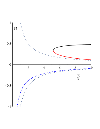
Figure 4: The solutions of the cubic equation (43) for $\bar{u}$ are plotted as functions of $|\bar{\ell}|$ in the case $\epsilon=1$. For $|\bar{\ell}|>3\sqrt{3}\approx 5.196$ the (positive) solutions are always two (solid curves) and they coalesce (to $u=1/3$, corresponding to the circular photon orbit at $r=3M$) when $\bar{\ell}=3\sqrt{3}$, but $\bar{u}$ is confined to the interval $(0,\bar{u}_{2}]$ along the trajectories, with the maximal value occurring at $\bar{u}=\bar{u}_{2}$ corresponding to the minimal value of the radius. The dotted curves correspond to the flat spacetime roots $\bar{u}=\pm{1}/{|\bar{\ell}|}$ which are approached in the limit $\epsilon\to 0$.

Integrating Eq. (40) for the case $\bar{\ell}>0$ to avoid sign complications leads to

$$\phi(\bar{u})=\mp\sqrt{\frac{2}{\bar{u}_{3}-\bar{u}_{1}}}{\rm EllipticF}\left(\sin\left(\frac{\chi}{2}\right),k\right)+{\rm const.}$$ (52)

with

$$\sin\left(\frac{\chi}{2}\right)=\sqrt{\frac{\bar{u}-\bar{u}_{1}}{\bar{u}_{2}-\bar{u}_{1}}}\,,\qquad k=\sqrt{\frac{\bar{u}_{2}-\bar{u}_{1}}{\bar{u}_{3}-\bar{u}_{1}}}\,,$$ (53)

where EllipticF is the incomplete elliptic integral of the first kind defined explicitly in Appendix B.

To fix the additive constant in Eq. (52), consider the limit $\bar{u}\to\bar{u}_{2}$ where $\chi\to\pi$ and hence

$$\phi(\bar{u}_{2})=\mp\sqrt{\frac{2}{\bar{u}_{3}-\bar{u}_{1}}}{\rm EllipticK}(k)+{\rm const.}$$ (54)

so that

$$\phi(\bar{u})-\phi(\bar{u}_{2})=\mp\sqrt{\frac{2}{\bar{u}_{3}-\bar{u}_{1}}}\left[{\rm EllipticF}\left(\sin\left(\frac{\chi}{2}\right),k\right)-{\rm EllipticK}(k)\right]\,,$$ (55)

where the lower positive sign applies to the incoming photon orbit for $\bar{\ell}>0$, and EllipticK is the complete elliptic integral of the first kind defined in Appendix B. Hereafter we will only consider the incoming case with the positive sign. This formula is directly analogous to the flat spacetime result (2) but where $\sin\chi/2$ is now related to $\phi$ by the more complicated composition with the elliptic function. In fact the $\epsilon\to 0$ limit of (55) with $k\to 0$ shows how this limit comes about, using the values ${\rm EllipticF}(\sin\chi/2,0)=\chi/2$, ${\rm EllipticK}(0)=\pi/2$. Note that this final result does not depend on our choice $\phi_{*}=0$ made for convenience of illustration, only that the photon orbit it describes has $\ell>0$.

Chandrasekhar Chandrasekhar:1985kt (see pag. 131, Eq. 260) chooses $\phi(\bar{u}_{2})=0$, i.e., sets $\phi=0$ at the “minimal distance.” Here $\phi(\bar{u}_{2})$ corresponds to the flat spacetime impact parameter $\phi^{(0)}(\bar{\ell})$, showing its explicit dependence on $\bar{\ell}$. This elliptic function relationship can be inverted to give $u$ as a function of $\phi$ using the Jacobi elliptic function JacobiSN($x,k$) which inverts EllipticF($x,k$), first giving

$$\sin\frac{\chi}{2}=\sqrt{\frac{\bar{u}-\bar{u}_{1}}{\bar{u}_{2}-\bar{u}_{1}}}={\rm JacobiSN}\left(\alpha(\phi),k\right)\,.$$ (56)

with

$$\alpha(\phi)=\sqrt{\frac{\bar{u}_{3}-\bar{u}_{1}}{2}}\left(\phi-\phi(\bar{u}_{2})\right)+{\rm EllipticK}(k)\,,$$ (57)

and then

$$\bar{u} = \bar{u}_{1}+(\bar{u}_{2}-\bar{u}_{1}){\rm JacobiSN}^{2}\left(\alpha(\phi),k\right)\,.$$ (58)

Note that setting $u=0$ in the right hand side of (55) for $\bar{\ell}>0$ and reversing its sign gives half the increase in $\phi$ over the entire photon orbit, so that by doubling this and subtracting $\pi$ gives the net scattering angle for the orbit. Fig. (5) shows this scattering angle as a function of the minimal distance for $r/M\geq 3$. This approaches infinity as the photon orbits wrap around the circular photon orbit at $r/M=3$.

At the point of reception $(r_{0}=\bar{u}_{0}^{-1},\phi_{0})$ of a photon making an observed angle $\beta_{0}$ with the azimuthal direction, (35) gives the value of $\ell$ for the incoming photon orbit

$$\bar{\ell}=\frac{\cos\beta_{0}}{\bar{u}_{0}\sqrt{1-2\bar{u}_{0}}}\,.$$ (59)

Then evaluating (55) at $\bar{u}=\bar{u}_{0}$, $\phi(\bar{u}_{0})=\phi_{0}$

$$\phi_{0}-\phi(\bar{u}_{2})=\sqrt{\frac{2}{\bar{u}_{3}-\bar{u}_{1}}}\left[{\rm EllipticF}\left(\sin\left(\frac{\chi_{0}}{2}\right),k\right)-{\rm EllipticK}(k)\right]\,,$$ (60)

this determines the value $\phi(\bar{u}_{2})$. Similarly at the point of emission $(\bar{r}_{*}=\bar{u}_{*}^{-1},\phi_{*})$, one has

$$\phi_{*}-\phi(\bar{u}_{2})=\sqrt{\frac{2}{\bar{u}_{3}-\bar{u}_{1}}}\left[{\rm EllipticF}\left(\sin\left(\frac{\chi_{*}}{2}\right),k\right)-{\rm EllipticK}(k)\right]\,.$$ (61)

For instance suppose we know that the point $P_{*}$ has $\phi_{*}=0$. Then Eq. (61) or its inverse Eq. (58) with $\phi_{*}=0$ determines $\bar{u}_{*}$.

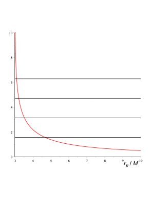
Figure 5: The scattering angle for the photon orbit as a function of the minimal radius $r_{0}$ along the photon orbit. The horizontal lines mark off multiples of $\pi/2$. For $\bar{r}_{0}=4.65$ this angle equals $\pi/2$ corresponding to a 90 degree change in direction, while at smaller radii where it exceeds $\pi$ the photon makes at least one loop around the black hole horizon.

Suppose for the sake of an explicit example, we fix a relativistic Schwarzschild timelike circular geodesic orbit at $r_{0}=8M$ ($\bar{u}_{0}=1/8$) in the corresponding flat spacetime with initially $r_{*{\rm(flat)}}=20M$ and pick the corresponding value $\phi_{0}=\phi^{(0)}=\arccos(2/5)\approx 66.4^{\circ}$, $\ell_{0{\rm(flat)}}=r_{0}$ (so that $\bar{\ell}_{0{\rm(flat)}}\bar{u}_{0}=1$) to be the last point $P_{1}=Q$ on the side of the orbit facing the emitter for $\phi>0$ (shown in Fig. 3 for the flat case) which receives the incoming photon with angle $\beta_{0}=0$, such that $1=\cos\beta_{0}=\ell_{0{\rm(flat)}}/r_{0}$ (and $\beta_{0*{\rm(flat)}}=-\phi_{0}$).

Next from $1=\cos\beta_{0}=\bar{\ell}_{0}\bar{u}_{0}\sqrt{1-2\bar{u}_{0}}$ calculate the corresponding Schwarzschild value $\bar{\ell}_{0}=16/\sqrt{3}\approx 9.24$ for that same incoming angle of $\beta_{0}=0$ for the curved orbit through this point $P_{1}$. Then using the null geodesic orbit equation (61) with $\phi(\bar{u}_{2})=\phi_{0}$ and $\phi_{*}=\phi(u_{*})=0$, calculate $r_{*}/M\approx 13.46=1/u_{*}$. $\phi_{*}=0$ corresponds to an incoming (captured) photon with $\ell=0$ (frontal zero aberration point in the orbit). Now one has the emitter point and the maximum negative acute angle $\beta_{0*}\approx-50.7^{\circ}$ for which photons will reach the circular orbit. Next calculate the minimum negative angle $\beta_{*\rm(cap)}\approx-69.1^{\circ}$ at which the photon is captured from $\cos\beta_{*\rm(cap)}=3\sqrt{3}\bar{u}_{*}\sqrt{1-2\bar{u}_{*}}$.

Pick an intermediate value $\beta_{*\rm(cap)}<\beta_{1*}<\beta_{0*}$ for a new photon orbit emitted from the point $P_{*}$, say $\beta_{1*}=-65^{\circ}$ with angular momentum $\bar{\ell}_{1}\approx 6.16$ determined by $\cos\beta_{1*}=\bar{\ell}_{1}\bar{u}_{*}\sqrt{1-2\bar{u}_{*}}$. Calculate the new angle $\phi_{1}\approx 17.1^{\circ}$ of reception and the corresponding incoming angle $-\pi/2<\beta_{1}\approx-55.8^{\circ}$.

Finally, to consider the time evolution of a given photon trajectory in spacetime, one has the explicit solution of Eq. (42) with the initial condition $t(\bar{u}_{*})=0$

$$t(\bar{u})=H(\bar{u})-H(\bar{u}_{*})\,,$$ (62)

where

$$H(\bar{u}) = -\frac{\bar{\ell}}{\bar{u}}\sqrt{\mathcal{V}_{(\bar{\ell},\epsilon)}(\bar{u})}$$ (63)

$$+C_{1}{\rm EllipticPi}\left(\sin\frac{\chi}{2},1-\frac{\bar{u}_{2}}{\bar{u}_{1}},k\right)$$

$$+C_{2}{\rm EllipticPi}\left(\sin\frac{\chi}{2},\frac{2(\bar{u}_{1}-\bar{u}_{2})}{2\bar{u}_{1}-1},k\right)$$

$$+C_{3}{\rm EllipticE}\left(\sin\frac{\chi}{2},k\right)+C_{4}{\rm EllipticF}\left(\sin\frac{\chi}{2},k\right)\,,$$

with

$$C_{1} = -\frac{4}{\sqrt{2}\bar{\ell}\bar{u}_{1}\sqrt{\bar{u}_{3}-\bar{u}_{1}}}\,,\quad C_{2}=\frac{4\sqrt{2}}{\bar{\ell}(2\bar{u}_{1}-1)\sqrt{\bar{u}_{3}-\bar{u}_{1}}}\,,$$

$$C_{3} = \sqrt{2}\bar{\ell}(\bar{u}_{3}-\bar{u}_{1})\,,\quad C_{4}=\frac{1}{\sqrt{2}\bar{\ell}}\frac{1}{\bar{u}_{1}\bar{u}_{2}\sqrt{\bar{u}_{3}-\bar{u}_{1}}}\,,$$ (64)

recalling the definitions (53) introduced above.

Imagining the curved orbit figure corresponding to the flat spacetime case illustrated Fig. 3, the horizontal direction depicted on the circular orbit at the maximal impact parameter cases still corresponds to photons arriving from spatial infinity. Compared to the celestial circle of the distant stars in the equatorial plane, the apparent direction of the point $P_{*}$ varies from $\beta=0$ at the lower point $Q$ in Fig. 3 to $\beta=\pi$ at the upper point $Q$ as one moves along the circular orbit.

The parallax angle of $P_{*}$ is equal to the angle made by the incoming photon with the horizontal direction $\phi=0$ which corresponds to $\beta=\pi/2-\phi_{0}$ at the lower point $Q$ for $\ell<0$ and $\beta=\pi/2+\phi_{0}$ at the upper point $Q$ for $\ell>0$. However, nonrelativistic discussions define the parallax angle in terms of the photons observed when the point $P_{2}$ of the orbit lies at the extreme antipodal points $\phi=\pm\pi/2$ on the circular orbit relative to the direction $\phi=0$. This requires a piecewise solution of the photon orbit to deal with the sign change after the minimal approach point $Q$ is reached inside the circular orbit. This leads to a more complicated discussion, which would describe the exact parallax for an emitter on the polar axis of the spherical coordinate system orthogonal to the equatorial plane.

3.2 Capture case

Orbits for $|\bar{\ell}|<3\sqrt{3}\approx 5.20$ are captured by the black hole so no minimal radius exists, and one must therefore choose initial conditions differently from the noncapture case in (54). The formulas (3.1) remain valid but the root $u_{1}$ remains real and negative, while the roots $u_{2}$, $u_{3}$ become complex conjugates. In the definition of $X$ in (47) the quantity $\theta_{X}$ vanishes at $|\bar{\ell}|=3\sqrt{3}$ and then becomes purely imaginary. We choose the initial condition $\phi(\bar{u}_{*})=0$ so that

$$\phi(\bar{u})=\sqrt{\frac{2}{\bar{u}_{3}-\bar{u}_{1}}}\left[{\rm EllipticF}\left(\sin\left(\frac{\chi}{2}\right),k\right)-{\rm EllipticF}\left(\sin\left(\frac{\chi_{*}}{2}\right),k\right)\right]\,.$$ (65)

For example, if $\bar{\ell}=5$ one finds $\bar{u}_{1}=-0.172$,$\bar{u}_{2}=0.336+0.0540i=\bar{u}_{3}^{*}$ and $\phi(\bar{u}_{0})\approx 16.3^{\circ}$.

4 The inverse problem

Given $r_{*}$, in order to determine the corresponding value $\phi_{0}=\phi(u_{2})$ for which the point $Q$ is on the circular orbit, one must first determine the value of $\ell>0$ from the condition (59) with $\beta_{0}=0$ and then setting $\phi_{*}=0$ in (61) with this value of $\ell$, one finds the corresponding value of $\phi(u_{2})$. In our above example, this leads to a parallax angle of $23.6^{\circ}$, the complement of the angle $\phi_{0}$ we started with.

Finally consider how to determine the radial position $r_{*}$ from two pairs of incoming data $(\phi,\beta)$ from the same point $P_{*}$, namely $(\phi_{1},\beta_{1})$ and $(\phi_{2},\beta_{2})$ at $r=r_{0}$ which immediately gives us the corresponding values $\bar{\ell}_{1}$ and $\bar{\ell}_{2}$ which determine the roots $\bar{u}_{i}(\bar{\ell})$ describing the incoming photon.

Suppose we represent Eq. (55) by

$$\phi(\bar{u})-\phi(\bar{u}_{2}(\bar{\ell}))=F(\bar{u},\bar{\ell})\,,$$ (66)

where $F(\bar{u},\bar{\ell})$ denotes symbolically the right-hand-side of that equation. Evaluating it first at $\bar{u}=\bar{u}_{0}$ for $\bar{\ell}_{1}$ and $\bar{\ell}_{2}$ we then solve for $\phi(\bar{u}_{2}(\bar{\ell}_{1}))$ and $\phi(\bar{u}_{2}(\bar{\ell}_{2}))$. Then using these known values, we evaluate this equation again at $\bar{u}=\bar{u}_{*}$ for $\phi(\bar{u}_{*})=\phi_{1}$ for $\bar{\ell}_{1}$ and $\phi(\bar{u}_{*})=\phi_{2}$ for $\bar{\ell}_{2}$. These two independent equations for the two unknowns $\bar{u}_{*}$, $\phi_{*}$ can be solved numerically.

We can use the data from our example as a test case to recover the coordinates of $P_{*}$. Starting from $(\phi_{1},\beta_{1})=(66.4^{\circ},0^{\circ})$ and $(\phi_{2},\beta_{2})=(21.6^{\circ},-48.1^{\circ})$ following the above steps, one easily finds indeed $r_{*}=13.4M$ and $\phi_{*}=0.00910^{\circ}$ keeping only 3 significant digits.

5 Targeting problem

Suppose both the emitter and receiver are in circular motion in the same plane. One can study the significantly more complicated problem of aiming an emitted photon in such a way as to hit the receiver. This requires including the time evolution of the photon. As a first step one can track a photon emitted at $t=0$, $\phi_{*}=0$ from the point $P_{*}$ on a circular geodesic orbit at radius $r_{*}=M/u_{*}>r_{0}$ (with angular velocity $\Omega_{\rm(em)}=\sqrt{M/r_{*}^{3}}$) and calculate the angle $\phi_{0}$ it arrives at the receiver at time $t=t_{1}$ in the circular orbit $\phi=\Omega_{\rm(rec)}t$ at radius $r_{0}=M/u_{0}$ (with angular velocity $\Omega_{\rm(rec)}=\sqrt{M/r_{0}^{3}}$).

Let $\phi(u,\ell)$, $t(u,\ell)$ describe the null geodesic from $P_{*}$ such that $\phi(u_{*},\ell)=0$, $t(u_{*},\ell)=0$. The condition that the photon arrive at the same angle and time as the receiver is

$$t_{1}\Omega_{\rm(rec)}=\phi(u_{0},\ell)\,,\quad t_{1}=t(u_{0},\ell)\,.$$ (67)

The ratio of these two relations then leads to

$$u_{0}^{3/2}=M\Omega_{\rm(rec)}=M\frac{\phi(u_{0},\ell)}{t(u_{0},\ell)}\,.$$ (68)

This can then be solved numerically for the value of $\ell$ required to fix the initial photon direction $\beta_{*}=\arccos(\bar{\ell}\bar{u}_{*}\sqrt{1-2\bar{u}_{*}})$.

Provided that the photon orbit can be described by the interval of $\ell>0$ values for a noncapture orbit, we can use the explicit elliptic function formulas derived above to determine the solution for $\ell$. In particular for the above noncapture example with $r_{0}=8M$, $r_{*}\approx 13.46M$ one finds $\bar{\ell}\approx 5.814$, $\beta_{*}\approx 66.5^{\circ}$, determining the photon orbit which arrives at the receiver at $\phi_{0}\approx 19.9^{\circ}$.

6 Concluding remarks

The investigation presented here shows that one can perform the strong field calculations of relativistic optics required to determine positions of photon emitters (like a star or satellite) from observations made by an observer in circular motion around a nonrotating compact object or black hole. Starting from the much simpler situation in flat spacetime optics for comparison, calculations are then performed for the corresponding Schwarzschild spacetime where both emitter and receiver are confined to the same plane. Given two observation points on the observer orbit, one can uniquely determine the location coordinates of an emitter fixed in the static grid of the spacetime. This analysis also shows concretely how one can solve the inverse problem of using photons to target a particular object in relative motion. By expanding exact formulas involving elliptic functions in the mass of the source of the gravitational field, one finds the corrections to the flat spacetime optics necessary to take into account spacetime curvature effects in the weak field case. Generalizations of these calculations to the full 3-dimensional spatial geometry in the Schwarzschild spacetime as well as to the case of a rotating Kerr spacetime will be considered in future work.

Appendix A The aberration map

The (nonlinear) aberration map describes the relationship between the apparent directions of a light ray as seen by two arbitrary observers in relative motion at the same spacetime point. These are purely special relativistic considerations in the tangent space valid both for any spacetime. Consider a photon with 4-momentum $P$ and unit relative velocities $\hat{\nu}(P,u)$ or $\hat{\nu}(P,U)$

$$P=E(P,u)[u+\hat{\nu}(P,u)]=E(P,U)[U+\hat{\nu}(P,U)]$$ (69)

as seen by two different observers with 4-velocities $u$ and

$$U=\gamma(U,u)[u+\nu(U,u)]=\gamma(U,u)[u+||\nu(U,u)||\hat{\nu}(U,u)]\,,$$ (70)

where in the last equation we have introduced the magnitude and the unit spatial direction of the relative velocity $\nu(U,u)=||\nu(U,u)||\hat{\nu}(U,u)$. Moreover, the inverse relations are easily written using the convenient but precise relative observer notation of Ref. Jantzen:1992rg , namely

$$u=\gamma(u,U)[U+\nu(u,U)]\,,$$ (71)

with $\gamma(u,U)=\gamma(U,u)=-U\cdot u$ and

$$-\nu(u,U)=\gamma(U,u)||\nu(U,u)||\,\left[\,||\nu(U,u)||\,u+\hat{\nu}(U,u)\right]\,.$$ (72)

Contracting Eq. (69) by $U$ one easily finds

$$E(P,U)=\gamma(U,u)[1-\nu(U,u)\cdot\hat{\nu}(P,u)]E(P,u)\,,$$ (73)

which can be rewritten in terms of the photon frequencies $\omega(P,u)=E(P,u)/\hbar$ and $\omega(P,U)=E(P,U)/\hbar$ leading to the formula (8) for the relativistic Doppler effect.

Instead projecting Eq. (69) orthogonally to $u$ leads to

$$P(u,U)\hat{\nu}(P,U)=\frac{E(P,u)}{E(P,U)}\hat{\nu}(P,u)-\gamma(U,u)\nu(U,u)\,,$$ (74)

where $P(u,U)=P(u)P(U)$ is the projection map from the local rest space of $U$ into that of $u$, and $P(u)^{\alpha}{}_{\beta}=\delta^{\alpha}{}_{\beta}+u^{\alpha}u_{\beta}$. Expanding the left-hand-side of this equation, namely $P(u,U)\hat{\nu}(P,U)=P(u)\hat{\nu}(P,U)=\hat{\nu}(P,U)+u[u\cdot\hat{\nu}(P,U)]$, and re-expressing the scalar product $u\cdot\hat{\nu}(P,U)$ replacing $\hat{\nu}(P,U)$ by

$$\hat{\nu}(P,U)=\frac{E(P,u)}{E(P,U)}[u+\hat{\nu}(P,u)]-U$$ (75)

implies

$$\hat{\nu}(P,U)-\nu(u,U)=\frac{E(P,u)}{E(P,U)}P(u,U)^{-1}\hat{\nu}(P,u)$$ (76)

or

$$\hat{\nu}(P,u)=\frac{E(P,U)}{E(P,u)}P(u,U)[\hat{\nu}(P,U)-\nu(u,U)]\,,$$ (77)

with its inverse relation obtained by exchanging $U$ and $u$,

$$\hat{\nu}(P,U)=\frac{E(P,u)}{E(P,U)}P(U,u)[\hat{\nu}(P,u)-\nu(U,u)]\,.$$ (78)

More familiar relations (for classical Doppler effect) are obtained decomposing the relative velocity $\hat{\nu}(P,U)$ into parts parallel and perpendicular to the direction $\hat{\nu}(u,U)$ of relative motion

$$\hat{\nu}(P,U)=\hat{\nu}(P,U)^{(\|)}+\hat{\nu}(P,U)^{(\perp)}\,,\,$$ (79)

with $\hat{\nu}(P,U)^{(\|)}=||\hat{\nu}(P,U)^{(\|)}||\hat{\nu}(u,U)$, and similarly

$$\hat{\nu}(P,u)=\hat{\nu}(P,u)^{(\|)}+\hat{\nu}(P,u)^{(\perp)}\,,\,$$ (80)

with $\hat{\nu}(P,u)^{(\|)}=||\hat{\nu}(P,u)^{(\|)}||\hat{\nu}(U,u)$. Re-expressing the relative projection in terms of the boost leads to the formulas

$$\hat{\nu}(P,U)^{(\perp)} = \gamma(U,u)^{-1}[1-\nu(U,u)\cdot\hat{\nu}(P,u)]^{-1}\hat{\nu}(P,u)^{(\perp)}\,,$$

$$\hat{\nu}(P,U)^{(\|)} = [1-\nu(U,u)\cdot\hat{\nu}(P,u)]^{-1}B_{\rm(lrs)}(u,U)[\hat{\nu}(P,u)^{(\|)}-\nu(U,u)]\,,$$ (81)

where we have introduced the boost map $B_{\rm(lrs)}(u,U)$ from the local rest space of $U$ to that of $u$ (see Eq. 4.22 of Ref. Jantzen:1992rg ) defined so that

$$[B_{\rm(lrs)}(u,U)S]^{\alpha}=\left[P(u)-\frac{\gamma(U,u)}{1+\gamma(U,u)}\nu(U,u)\otimes\nu(U,u)\right]{}^{\alpha}{}_{\beta}[P(u,U)S]^{\beta}$$ (82)

for any vector $S$ belonging to the local rest space of $U$.

For the special case

$$\hat{\nu}(P,u)^{(\|)}=0\ ,\qquad||\hat{\nu}(P,u)^{(\perp)}||=1$$ (83)

of a light ray orthogonal to the relative motion as seen by $u$, one has the familiar result

$$\tan\theta_{U}={||\hat{\nu}(P,U)^{(\|)}||\over||\hat{\nu}(P,U)^{(\perp)}||}=\gamma(U,u)||\nu(U,u)||$$ (84)

for the angle away from the perpendicular direction as seen by $U$, using the fact that boosts preserve lengths.

For the present application to the circularly rotating observer $U$ and the static observer $n$, let

$$U=\gamma(U,n)[n+||\nu(U,n)||e_{\hat{\phi}}]\,,\quad E_{\hat{\phi}}=\gamma(U,n)[||\nu(U,n)||n+e_{\hat{\phi}}]\,.$$ (85)

The arriving photon can be viewed by either observer, defining the azimuthal angle of reception by

$$\hat{\nu}(P,U)^{\hat{\phi}}=\hat{\nu}(P,U)\cdot E_{\hat{\phi}}=\cos\beta_{U}\,,\quad\hat{\nu}(P,n)^{\hat{\phi}}=\hat{\nu}(P,n)\cdot e_{\hat{\phi}}=\cos\beta_{n}\,.$$ (86)

From Eq. (75) with $u=n$, contracting both sides with $E_{\hat{\phi}}$, one finds

$$\cos\beta_{U}=\frac{\cos\beta_{n}-||\nu(U,n)||}{1-\cos\beta_{n}||\nu(U,n)||}\,,$$ (87)

where

$$||\nu(U,n)||=\frac{r_{0}\Omega}{\sqrt{1-2M/r_{0}}}\equiv\Omega R_{\rm(lie)}^{0}\,.$$ (88)

This is the aberration map at the reception point whose inverse is needed to transform the observed angle to the static observer value required for the computations.

Appendix B Approximate formulas

Here we summarize the linear expansion in $\epsilon$ of this analysis, noting again that setting $\epsilon=1$ in the resulting expressions is equivalent to the weak field limit $M/r\ll 1$ of the exact expressions. This describes the corrections due to the curvature of spacetime.

We use the following definitions Gradshteyn of the complete and incomplete elliptic integrals of the first kind ${\rm EllipticK}(k)$ and ${\rm EllipticF}(\varphi,k)$ defined respectively by

$${\rm EllipticF}(\varphi,k) = \int_{0}^{\varphi}\frac{dz}{\sqrt{1-k^{2}\sin^{2}z}}\,,\quad{\rm EllipticK}(k)={\rm EllipticF}(\pi/2,k)\,.$$ (89)

The following expansions of elliptic functions and their parameters are useful.

$${\rm EllipticF}\left(x_{0}+\epsilon x_{1},k_{1/2}\epsilon^{1/2}+k_{3/2}\epsilon^{3/2}\right)$$

$$\qquad=\arcsin x_{0}+\frac{\epsilon}{4}\left[k_{1/2}^{2}\arcsin x_{0}+\frac{x_{1}}{\sqrt{1-x_{0}^{2}}}-x_{0}k_{1/2}^{2}\sqrt{1-x_{0}^{2}}\right]+O(\epsilon^{2})\,,$$

$${\rm EllipticK}(k_{1/2}\epsilon^{1/2}+k_{3/2}\epsilon^{3/2})=\frac{\pi}{2}\left(1+\frac{1}{4}k_{1/2}^{2}\epsilon\right)+O(\epsilon^{2})\,.$$ (90)

From the definition (53), it follows from (3.1) that the parameter $k\to 0$ as $\epsilon\to 0$ and $k^{2}=1$ when $\bar{\ell}=3\sqrt{3}\epsilon$ while, for large $\bar{\ell}$

$$k^{2}=\frac{4\epsilon}{\bar{\ell}}-\frac{8\epsilon^{2}}{\bar{\ell}^{2}}+\frac{50\epsilon^{3}}{\bar{\ell}^{3}}+O\left(\frac{\epsilon^{4}}{\bar{\ell}^{4}}\right)\,.$$ (91)

Moreover, approximate expressions for $\sin\chi/2$ and ${\rm EllipticK}(k)$ are the following

$$\sin\frac{\chi}{2}=\sqrt{\frac{\bar{\ell}\bar{u}}{2\epsilon}}\left(1+\frac{1}{2\bar{u}}\frac{\epsilon}{\bar{\ell}}-\frac{1+4\bar{u}+10\bar{u}^{2}}{8\bar{u}^{2}}\frac{\epsilon^{2}}{\bar{\ell}^{2}}+\frac{1+4\bar{u}+10\bar{u}^{2}}{16\bar{u}^{3}}\frac{\epsilon^{3}}{\bar{\ell}^{3}}\right)+O\left(\epsilon^{7/2}\right)\,,$$

$${\rm EllipticK}(k)=\frac{\pi}{2}\left(1+\frac{\epsilon}{\bar{\ell}}+\frac{1}{4}\frac{\epsilon^{2}}{\bar{\ell}^{2}}\right)+O(\epsilon^{3})\,.$$ (92)

Using the approximate formula (B) in Eq. (54) with the plus sign for the incoming photon, we find for $\bar{\ell}>0$

$$\phi(\bar{u})-\phi(\bar{u}_{2})=\left(2\arcsin\left(\sqrt{\frac{1+\bar{u}\bar{\ell}}{2}}\right)-\frac{\epsilon}{\bar{\ell}}\left[\sqrt{1-\bar{u}^{2}\bar{\ell}^{2}}+\frac{1}{\sqrt{1-\bar{u}^{2}\bar{\ell}^{2}}}\right]\right)+O(\epsilon^{2})$$ (93)

or using the identity

$$\arccos x=\pi-2\arcsin\left(\sqrt{\frac{1+x}{2}}\right)\,,$$ (94)

we get

$$\phi(\bar{u})-\phi(\bar{u}_{2})=\Phi_{(\bar{\ell},\epsilon)}(\bar{u})+O(\epsilon^{2})\,,$$ (95)

where

$$\Phi_{(\bar{\ell},\epsilon)}(\bar{u})=\arccos(\bar{u}\bar{\ell})+\frac{\epsilon}{\bar{\ell}}\left(\sqrt{1-\bar{u}^{2}\bar{\ell}^{2}}+\frac{1}{\sqrt{1-\bar{u}^{2}\bar{\ell}^{2}}}\right)\,.$$ (96)

Finally $\ell$ is itself a function of $\epsilon$ when expressed as a function of the minimal orbit radius $R$ using Eq. (33) with $M$ replaced by $\epsilon M$. This further expansion of Eq. (96) leads to

$$\Phi_{(\bar{\ell},\epsilon)}(\bar{u})=\arccos(\bar{u}\bar{R})+\frac{2}{\bar{R}}\frac{1-\frac{\bar{u}\bar{R}}{2}-\frac{\bar{u}^{2}\bar{R}^{2}}{2}}{\sqrt{1-\bar{u}^{2}\bar{R}^{2}}}\epsilon+O(\epsilon^{2})\,,$$ (97)

which coincides with Eq. (2) of Ref. Arifov:1969 .

As in the flat spacetime case, if two photons arrive at a circle of radius $r_{0}=M/\bar{u}_{0}$ at two successive angles $\phi_{1}$ and $\phi_{2}$ with parameters $\bar{\ell}_{1}$ and $\bar{\ell}_{2}$ from the same point of emission $(r_{*},\phi_{*})$, we can calculate the minimal distance angles $\phi^{(0)}(\bar{\ell}_{1})$ and $\phi^{(0)}(\bar{\ell}_{2})$, for example $\phi_{1}-\phi^{(0)}(\bar{\ell}_{1})=\Phi_{(\bar{\ell}_{1},\epsilon)}(\bar{u}_{0})+O(\epsilon^{2})\,,$ and a similar relation for the second photon. Then once we have $\phi_{\bar{\ell}_{1}}$ and $\phi_{\bar{\ell}_{2}}$ known in terms of $(r_{0},\phi_{1},\phi_{2},\bar{\ell}_{1},\bar{\ell}_{2})$, we have

$$\phi_{*}-\phi^{(0)}(\bar{\ell}_{1})=\Phi_{(\bar{\ell}_{1},\epsilon)}(\bar{u}_{*})+O(\epsilon^{2})\,,$$ (98)

$$\phi_{*}-\phi^{(0)}(\bar{\ell}_{2})=\Phi_{(\bar{\ell}_{2},\epsilon)}(\bar{u}_{*})+O(\epsilon^{2})\,.$$ (99)

Subtracting these two relations leads to

$$\delta_{12} = \phi^{(0)}(\bar{\ell}_{2})-\phi^{(0)}(\bar{\ell}_{1})=\Phi_{(\bar{\ell}_{1},\epsilon)}(\bar{u}_{*})-\Phi_{(\bar{\ell}_{2},\epsilon)}(\bar{u}_{*})+O(\epsilon^{2})\,,$$ (100)

which can be solved for $\bar{u}_{*}$, leading to

$$\bar{u}_{*} = \frac{|\sin\delta_{12}|}{\sqrt{\bar{\ell}_{1}^{2}+\bar{\ell}_{2}^{2}-2\bar{\ell}_{1}\bar{\ell}_{2}\cos\delta_{12}}}+\epsilon\frac{2(\bar{\ell}_{1}^{2}+\bar{\ell}_{2}^{2})\cos\delta_{12}-\bar{\ell}_{1}\bar{\ell}_{2}(1+3\cos^{2}\delta_{12})}{\bar{\ell}_{1}\bar{\ell}_{2}(\bar{\ell}_{1}^{2}+\bar{\ell}_{2}^{2}-2\bar{\ell}_{1}\bar{\ell}_{2}\cos\delta_{12})}$$ (101)

$$+O(\epsilon^{2})\,.$$

This result can be substituted in either of the previous two relations to determine $\phi_{*}$. Higher-order approximation formulas can be obtained straightforwardly.

References

(1)
C. Darwin,
“The gravity field of a particle,
Proc. Roy. Soc. A 249, 180 (1959).
(2)
C. W. Misner, K. S. Thorne and J. A. Wheeler,
“Gravitation,”
San Francisco 1973, 1279p
(3)
J.P. Luminet,
“Image of a spherical black hole with thin accretion disk,”
Astron. Astrophys. 75, 228 (1979).
(4)
S. Chandrasekhar,
“The mathematical theory of black holes,”
Oxford, UK: Clarendon(1985), p. 646.
(5)
A. Cadez and U. Kostic,
“Optics in the Schwarzschild Spacetime,”
Phys. Rev. D72, 104024 (2005).
(6)
G. Munoz,
“Orbits of massless particles in the Schwarzschild metric: Exact solutions,”
Am. J. Phys. 82, 564 (2014)
doi: 10.1119/1.4866274
(7)
L.Y. Arifov and R.K. Kadyev,
“The Relativistic Theory of Annual Parallaxes,”
Sov. Astronomy 12, 882 (1969).
(8)
O. Semerák,
“Approximating light rays in the Schwarzschild field,”
Astrophys. J. 800, 77 (2015)
doi:10.1088/0004-637X/800/1/77
[arXiv:1412.5650 [astro-ph.HE]].
(11)
D. Bini, P. Carini and R. T. Jantzen,
“The Intrinsic derivative and centrifugal forces in general relativity. 1. Theoretical foundations,”
Int. J. Mod. Phys. D 6, 1 (1997)
doi:10.1142/S0218271897000029
[gr-qc/0106013].
(12)
D. Bini, P. Carini and R. T. Jantzen,
“The Intrinsic derivative and centrifugal forces in general relativity. 2. Applications to circular orbits in some familiar stationary axisymmetric space-times,”
Int. J. Mod. Phys. D 6, 143 (1997)
doi:10.1142/S021827189700011X
[gr-qc/0106014].
(13)
R. T. Jantzen, P. Carini and D. Bini,
“The Many faces of gravitoelectromagnetism,”
Annals Phys. 215, 1 (1992)
doi:10.1016/0003-4916(92)90297-Y
[gr-qc/0106043].
(14)
I. S. Gradshteyn and I. M. Ryzhik,
“Table of Integrals, Series, and Products,” Ed. by A. Jeffrey
and D. Zwillinger, Academic Press, New York, 6th edition, 2000.