The Einstein dark energy model

Abstract

In 1919 Einstein tried to solve the problem of the structure of matter by assuming that the elementary particles are held together solely by gravitational forces. In addition, Einstein also assumed the presence inside matter of electromagnetic interactions. Einstein showed that the cosmological constant can be interpreted as an integration constant, and that the energy content of the Universe should consist of 25% gravitational energy, and 75% electromagnetic energy. In the present paper we reinterpret Einstein’s elementary particle theory as a vector type dark energy model, by assuming a gravitational action containing a linear combination of the Ricci scalar and the trace of the matter energy-momentum tensor, as well as a massive self-interacting vector type dark energy field, coupled with the matter current. Since in this model the matter energy-momentum tensor is not conserved, we interpret these equations from the point of view of the thermodynamics of open systems as describing matter creation from the gravitational field. In the vacuum case the model admits a de Sitter type solution. The cosmological parameters, including Hubble function, deceleration parameter, matter energy density are obtained as a function of the redshift by using analytical and numerical techniques, and for different values of the model parameters. For all considered cases the Universe experiences an accelerating expansion, ending with a de Sitter type evolution.

I Introduction

After proposing a static model of the Universe, based on the introduction of the cosmological constant in the gravitational field equations Ein1 , Einstein tried to solve the problem of the structure of the elementary particles Ein2 . Adopting the basic assumption that material particles are bound together only by the gravitational force, depending on the metric tensor $g_{\mu\nu}$ and its derivatives, Einstein considered that the mass-energy structure of the elementary particles is described by an energy-momentum tensor of the Maxwell type, $S_{\mu\nu}$, constructed from the electromagnetic fields $F_{\mu\nu}$, which should be proportional with a differential expression of second order formed from the metric tensor coefficients (a linear combination of the Ricci and metric tensors). Hence Einstein proposed as the basic equation describing the properties of elementary particles the equation Ein2

$$R_{\mu\nu}+\bar{\lambda}g_{\mu\nu}R=\kappa^{2}S_{\mu\nu},$$ (1)

where $\bar{\lambda}$ is a constant, and $\kappa^{2}=8\pi G/c^{4}$ is the gravitational coupling constant. Since $S_{\mu}^{\mu}=0$, $\bar{\lambda}$ can be determined by taking the trace of Eq. (1) as $\bar{\lambda}=-1/4$, and thus Einstein’s equation (1) becomes

$$R_{\mu\nu}-\frac{1}{4}g_{\mu\nu}R=\kappa^{2}S_{\mu\nu}.$$ (2)

Moreover, Einstein assumed that the electromagnetic field satisfy Maxwell’s equations. Thus, by taking the covariant derivative of Eq. (2) we obtain

$$\frac{1}{4}\nabla_{\mu}R=-\frac{\kappa^{2}}{c}F_{\mu\nu}j^{\nu},$$ (3)

where $j^{\nu}$ is the electric current. Eq. (3) shows that the Coulomb repulsive forces are held in equilibrium by a gravitational pressure, thus assuring the stability of elementary particles. In the vacuum outside the elementary particle, and in the absence of charges, Eq. (3) gives

$$R=R_{0}=\mathrm{constant}.$$ (4)

At this moment Einstein did proceed to the determination of the matter energy-momentum tensor. He assumed that the gravitational field equations containing the cosmological constant,

$$R_{\mu\nu}-\frac{1}{2}g_{\mu\nu}R+\Lambda g_{\mu\nu}=\kappa^{2}T_{\mu\nu},$$ (5)

also remain valid. For the free space, in the absence of matter, Eq. (5) gives $R=4\Lambda$, and by comparison with Eq. (4), it follows that $\Lambda=R_{0}/4$. This result represents one of the main advantages of this approach, since it shows that the cosmological constant may not be a characteristic of the fundamental law of gravity, but an integration constant. Hence Eq. (5) becomes

$$G_{\mu\nu}+\frac{R_{0}}{4}g_{\mu\nu}=\kappa^{2}T_{\mu\nu},$$ (6)

giving

$$\kappa^{2}T=\left(R_{0}-R\right),$$ (7)

while Eq. (2) can be reformulated as

$$G_{\mu\nu}+\frac{1}{4}Rg_{\mu\nu}=\kappa^{2}S_{\mu\nu}.$$ (8)

Comparison of the above equations shows that

$$T_{\mu\nu}=S_{\mu\nu}+\frac{1}{4\kappa^{2}}\left(R_{0}-R\right)g_{\mu\nu}.$$ (9)

Einstein Ein2 interpreted the tensor $T_{\mu\nu}$ as the energy-momentum tensor of ”matter”. The ”matter” energy density therefore consists of two parts, the first one originating from the electromagnetic field, while the second one describes the gravitational contribution. From Eq. (9) we obtain

$$S_{\mu\nu}=T_{\mu\nu}-\frac{1}{4}Tg_{\mu\nu},$$ (10)

where $T=T_{\mu}^{\mu}$, and hence the field equation (2) can be reformulated as

$$R_{\mu\nu}-\frac{1}{4}g_{\mu\nu}R=\kappa^{2}\left(T_{\mu\nu}-\frac{1}{4}Tg_{\mu\nu}\right).$$ (11)

In the following we will call the field equations (11) the geometry-matter symmetric Einstein equations. For a dust Universe with $T_{0}^{0}=\rho$, where $\rho$ is the matter density, we have $S_{0}^{0}=3\rho/4$, and $S_{i}^{i}=-\rho/4$, $i=1,2,3$, respectively. Hence Einstein’s elementary particle theory made the remarkable prediction that the energy of the Universe is 75% (3/4) electromagnetic, and 25% (1/4) gravitational in its origin.

Einstein’s approach to the structure of the matter, did attract very little attention p1 ; p2 , even that it was sometimes briefly mentioned as a way to solve the cosmological constant problem, by interpreting it as an integration constant Wein . A theory in which the electromagnetic type energy-momentum tensor in Eq. (1) is substituted by the ordinary matter energy-momentum tensor, $S_{\mu\nu}\rightarrow T_{\mu\nu}$, so that

$$R_{\mu\nu}+\bar{\lambda}g_{\mu\nu}R=\kappa^{2}T_{\mu\nu},$$ (12)

was proposed by Rastall Rastall . In this theory the matter energy-momentum tensor is no longer conserved, and $\nabla_{\mu}T_{\nu}^{\mu}=\lambda\nabla_{\nu}R$, $\lambda=\mathrm{constant}$. Hence Rastall’s theory implies matter creation from the gravitational field. Different physical aspects of the Rastall theory, and its astrophysical and cosmological implications have been investigated recently in R1 ; R2 ; R3 ; R3a ; R4 ; R5 ; R6 ; R7 ; R8 ; R9 ; R10 . However, in Ri it was shown that the Rastall theory is just a particular case of the $f(R,T)$ gravity theory frt1 , where $T$ is the trace of the energy-momentum tensor, a modified gravity theory which is essentially based on a non-minimal geometry-matter coupling, which was investigated in frt2 ; frt3 ; frt4 ; frt5 ; frt6 ; frt7 ; frt8 ; frt9 ; frt10 ; frt11 ; frt12 . Several other alternative gravitational theories involving geometry-matter couplings have also been proposed, and extensively investigated in the physical literature, like, for example, the $f\left(R,L_{m}\right)$ modified gravity theory, where $L_{m}$ is the matter Lagrangian frlm1 ; frlm2 ; frlm3 ; frlm4 , the Weyl-Cartan modified gravity theories WCW ; nima , hybrid metric-Palatini $f(R,\tilde{R})$ gravity theory hpm1 ; hpm2 ; hpm3 , where $\tilde{R}$ is the Ricci scalar formed from a connection independent of the metric, the $f(R,T,R_{\mu\nu}T^{\mu\nu})$ gravity theory frtmu1 ; frtmu2 , or the $f(T,\tilde{T})$ gravity theory fttt , in which a coupling between the torsion scalar $\tilde{T}$ and the trace of the matter energy-momentum tensor is introduced. For a review of some modified gravity models and their cosmological implications see rr9 .

The dark energy problem is a fundamental problem in present day theoretical physics. A large number of cosmological studies, which were initiated by the study of the high redshift Type Ia Supernovae 1n ; 2n , have convincingly proven that the cosmological model according to which the Universe should decelerate due to its own gravitational attraction is not realized in nature. Cosmological observations have in fact convincingly shown that sometimes in the past, at a redshift of around $z\approx 0.5$, the Universe did experience a smooth transition to a de Sitter type accelerated expansionary phase 1n ; 2n ; 3n ; 4n . To fully explain these unexpected observational results a deep change in our understanding of the cosmological evolution, and of its theoretical basis, Einstein’s theory of general relativity, is necessary. Hence, in order to explain the present day observations in cosmology, and the mysterious and puzzling large scale behavior of the Universe, many new interesting theoretical ideas and models have been proposed recently, including loop quantum cosmology, bouncing cosmological models, string theoretical approaches, or general scalar-tensor cosmological models with up to second-order derivatives in the field equations rr1 ; rr2 ; rr3 ; rr4 ; rr5 . Presently, from both theoretical and observational points of view, there is an almost general consensus in the scientific community, which we may call generally as the ”standard paradigm of the recent cosmological acceleration” PeRa03 ; Pa03 ; rr6 ; rr7 . According to this new paradigm, all cosmological observations can be easily understood and interpreted theoretically once we assume the existence of a new and major component in the overall content of the Universe, called dark energy rr6 ; rr7 . Hence, once the non-evolving dark energy becomes the dominant component in the Universe, it also begins to control its evolutionary expansionary dynamics, thus determining the smooth transition to the de Sitter type accelerated stage that characterizes the late phases of the evolution of the Universe rr8 . Present day observations have also provided extremely powerful constraints on the important cosmological parameter $w=p/\rho$, where $p$ is the total pressure and $\rho$ is the total density of the Universe, which provides detailed information on the temporal behavior of the equation of state of the cosmological fluid rr8 . The analysis of the observational data on $w$ show that it is lying somewhere in the numerical range $-1\leq w<-1/3$ acc ; acc1 ; acc2 ; acc3 ; acc4 . The type-Ia supernova observations, Cosmic Microwave Background, large-scale structure, Hubble measurements, and baryon acoustic oscillations show that the concordance cosmological constant model, with $w=-1$ is still safely consistent with these observational data at the 68% confidence level acc4 . Recent results, based on full-mission Planck observations of temperature and polarization anisotropies of the Cosmic Microwave Background Radiation indicate, from the Planck temperature and lensing data, that the matter density parameter of the Universe is around $\Omega_{m}\approx 0.31$, giving a dark energy density parameter of the order of $\Omega_{\Lambda}\approx 0.70$ Planck .

There are a huge number of proposals to explain the dark energy (see, for example, the reviews PeRa03 ; Pa03 ; rr6 ; rr7 ). One possibility is that dark energy consists of quintessence, a slowly-varying, spatially inhomogeneous component of the Universe 8 . The idea of quintessence can be implemented theoretically by assuming that it is the energy associated with a scalar field $Q$, having a non-zero self-interaction potential $V(Q)$. When the potential energy density of the scalar field is greater than the kinetic one, the pressure $p=\dot{Q}^{2}/2-V(Q)$ associated to the scalar field $Q$-field is negative, thus leading to the possibility of the existence of an accelerated expansionary phase. Several cosmological models, based on the quintessence idea, have been intensively investigated in the physical literature (for a review see Tsu ).

The possible interaction between the dark energy and the dark matter components of the Universe has been considered within the framework of irreversible thermodynamics of open systems with matter creation/annihilation in H1 . The possibility that the cosmological anisotropy may arise as an effect of the non-comoving dark matter and dark energy has also been investigated H2 .

Dark energy models with nonstandard scalar fields, such as phantom scalar fields and Galileons, which can have bounce solutions and dark energy solutions with $w<-1$ have also been considered as an explanation of the late acceleration of the Universe gal1 ; gal2a ; gal2b ; gal2c ; gal3 ; gal4 ; gal5 . For a review of scalar field theories whose field equations are second order, and with second-derivative Lagrangians see Rub .

Scalar fields $\phi$ that are minimally coupled to gravity with a negative kinetic energy, which are known as “phantom fields”, have been introduced in phan1 . The energy density and pressure of a phantom scalar field are given by $\rho_{\phi}=-\dot{\phi}^{2}/2+V\left(\phi\right)$ and $p_{\phi}=-\dot{\phi}^{2}/2-V\left(\phi\right)$, respectively. The properties of phantom cosmological models have been investigated in phan2a ; phan2b ; phan2c ; phan2d ; phan3 ; phan4 .

An alternative to the scalar field dark energy models is represented by the vector type dark energy models, and their generalizations, in which dark energy is described by a vector field minimally coupled to gravity v1 ; v1a ; v1b ; v1c ; v1d ; v1e ; v1f ; v1g ; v1h ; v1i ; v1j ; v1k ; v1l ; v1m , a vector field non-minimally coupled to gravity v2 ; v2a ; v2b ; v2c ; v2d , or by some extended vector field models v3 ; v4 . The action for the non-minimally massive vector field coupled to gravity is given by v2

$$S=- \int d^{4}x\sqrt{-g}\Bigg{[}\frac{R}{2}+\frac{1}{16\pi}F_{\mu\nu}F^{\mu\nu}-\frac{1}{2}\mu_{\Lambda}^{2}A_{\mu}A^{\mu}$$

$$+\omega A_{\mu}A^{\mu}R+\eta A^{\mu}A^{\nu}R_{\mu\nu}+L_{m}\Bigg{]},$$ (13)

where $A^{\mu}\left(x^{\nu}\right)$, $\mu,\nu=0,1,2,3$ is the four-potential of the dark energy, which is allowed to couple non-minimally to gravity. $\mu_{\Lambda}$ denotes the mass of the massive cosmological vector field, while $\omega$ and $\eta$ are dimensionless coupling parameters. The vector type dark energy field tensor is defined as $F_{\mu\nu}=\nabla_{\mu}A_{\nu}-\nabla_{\nu}A_{\mu}$. So called ”superconducting” dark energy models, combining vector and scalar fields in a gauge invariant way, were considered in S1 ; S2 .

It is the goal of the present paper to reformulate Einstein’s theory of ”elementary particles” as a dark energy model. More specifically, we assume that the vector field $S_{\mu\nu}$ in Einstein’s theory represents a vector type dark energy, and not the standard electromagnetic field. Moreover, the model is extended from the description of the matter particles to the entire Universe. In order to obtain the field equation of the model, we adopt a Lagrangian that is reminiscent of the $f(R,T)$ theory of gravity frt1 , and contains a linear combination of the Ricci scalar and of the trace of the energy-momentum tensor. Moreover, we assume that the self-interacting dark energy tensor field $C_{\mu\nu}$ can be defined in terms of the dark energy massive vector potential $\Lambda_{\mu}$. A coupling between the matter current and the dark energy vector potential is also assumed.

The Einstein dark energy model field equations have the interesting property that the matter energy-momentum tensor is not conserved. We investigate and discuss this property from the perspective of the thermodynamics of open systems, in which the particle number is not conserved. Therefore the Einstein dark energy model may describe particle creation at a fundamental level. The particle creation rates, the creation pressure, as well as the entropy and temperature evolutions of the newly created particles are explicitly obtained with the use of a covariant formalism.

In order to investigate the cosmological evolution of the Universe we adopt a specific form of the dark energy vector potential. The cosmological equations, representing generalizations of the standard Friedmann equations, are formulated in a dimensionless form, and the redshift $z$ is adopted as the independent variable. For the vacuum case we show that the model admits a de Sitter type solution. We consider in detail two cosmological models, the conservative model, in which we impose the conservation of the matter energy-momentum tensor, and the general case, in which no specific assumptions on the physics of the system are made. In both cases we consider in detail the redshift evolution of the basic cosmological parameters (Hubble function, scale factor, deceleration parameter, matter energy density, and vector field potential, respectively), by using both analytical and numerical techniques. In both models the Universe enters in an accelerating phase, with the deceleration parameter taking negative values, at $z\approx 0.5$. Depending on the numerical values of the model parameters we can obtain a large range for the present day (negative) deceleration parameter.

The present paper is organized as follows. The variational principle of the Einstein dark energy model is introduced in Section II, and the corresponding field equations are derived. The thermodynamic interpretation of the dark energy model in the framework of the irreversible thermodynamics of open systems is discussed in Section III. The cosmological evolution equations of the Einstein dark energy model are written down in Section IV, and their dimensionless form is also obtained. The existence of the de Sitter solution is also proven. The general evolution of the Universe for a specific choice of the dark energy vector potential is investigated in Section V for both the conservative and nonconservative cases, by using analytical and numerical techniques. It is shown that in the presence of a self-interacting potential of the dark energy field the Universe ends in a de Sitter phase in both conservative and non-conservative cases. Finally, we discuss and conclude our results in Section VI.

II The Einstein dark energy model

In the present Section we present the basic gravitational field equations for the Einstein dark energy model, and derive some of its basic theoretical consequences.

II.1 The gravitational field equations

We assume that the Universe is filled with a cosmological vector field, which is described by a four-potential $\Lambda_{\mu}\left(x^{\nu}\right)$, $\mu,\nu=0,1,2,3$. From the dark energy vector potential, in analogy with electrodynamics, we define the dark energy field tensor

$$C_{\mu\nu}=\nabla_{\mu}\Lambda_{\nu}-\nabla_{\nu}\Lambda_{\mu}.$$ (14)

The dark energy field tensor identically satisfies the Maxwell type equations

$$\nabla_{\lambda}C_{\mu\nu}+\nabla_{\mu}C_{\nu\lambda}+\nabla_{\nu}C_{\lambda\mu}=0.$$ (15)

Furthermore, we assume that the dark energy field tensor $\Lambda_{\mu}$ is coupled to the ordinary matter current $j^{\mu}=\rho u^{\mu}$, where $\rho$ is the matter energy-density, and $u^{\mu}$ is the four-velocity of the cosmological flow, satisfying the normalization condition $u_{\mu}u^{\mu}=-1$.

We define the energy-momentum tensor $T_{\mu\nu}$ of the matter as

$$T_{\mu\nu}=-\frac{2}{\sqrt{-g}}\frac{\partial\left(\sqrt{-g}\mathcal{L}_{m}\right)}{\partial g^{\mu\nu}},$$ (16)

where $\mathcal{L}_{m}$ is the Lagrangian of the total (ordinary baryonic plus dark) matter. For ordinary matter, characterized, from a thermodynamic point of view, by its energy density $\rho$ and thermodynamic pressure $p$ only, the energy momentum tensor is given by

$$T_{\mu\nu}=\left(\rho+p\right)u_{\mu}u_{\nu}+pg_{\mu\nu}.$$ (17)

In the following by $T$ we denote the trace of the matter energy-momentum tensor.

Then the Einstein dark energy model can be derived from the following action

$$\tilde{S} =\int\sqrt{-g}d^{4}x\Bigg{[}\left(1-\beta_{1}\right)\frac{R}{2\kappa^{2}}+\frac{\beta_{2}}{2}T-\frac{1}{4}C_{\mu\nu}C^{\mu\nu}$$

$$-\frac{m^{2}}{2}\Lambda_{\mu}\Lambda^{\mu}-V\left(\Lambda^{2}\right)-\frac{\alpha}{2}j^{\mu}\Lambda_{\mu}+\mathcal{L}_{m}\Bigg{]},$$ (18)

where $\beta_{1}$, $\beta_{2}$, $m$ and $\alpha$ are constants.

The energy-momentum tensor $S_{\mu\nu}$ of the dark energy field, is constructed, by analogy with classical electrodynamics, as LaLi

$$S_{\mu\nu}=C_{\mu\alpha}C_{\nu}^{~{}\alpha}-\frac{1}{4}g_{\mu\nu}C_{\alpha\beta}C^{\alpha\beta},$$ (19)

with the property $S_{\mu}^{\mu}=0$.

By varying the gravitational action with respect to the metric tensor $g^{\mu\nu}$ it follows that the cosmological evolution of the Universe in the presence of a vector type dark energy is described by the generalized Einstein gravitational field equations,

$$\frac{(1-\beta_{1})}{\kappa^{2}}G_{\mu\nu}-S_{\mu\nu}-m^{2}\left(\Lambda_{\mu}\Lambda_{\nu}-\frac{1}{2}\Lambda^{2}g_{\mu\nu}\right)+$$

$$Vg_{\mu\nu}-2V^{\prime}\Lambda_{\mu}\Lambda_{\nu}-\frac{1}{2}\alpha\,p\,\left(u_{\mu}u_{\nu}+g_{\mu\nu}\right)\,u^{\alpha}\Lambda_{\alpha}$$

$$=(1+\beta_{2})T_{\mu\nu}-\beta_{2}\,\left(\mathcal{L}_{m}-\frac{1}{2}T\right)g_{\mu\nu},$$ (20)

where $V^{\prime}=dV/d\Lambda^{2}$. In obtaining the above equation we have used the variation of $T$ and $j^{\alpha}\Lambda_{\alpha}$ as (for the proof of these relations see frtmu1 and v3 , respectively)

$$\delta(\sqrt{-g}T)=-\sqrt{-g}\left[T_{\alpha\beta}+\left(\frac{1}{2}T-\mathcal{L}_{m}\right)g_{\alpha\beta}\right]\delta g^{\alpha\beta},$$ (21)

and

$$\delta( \sqrt{-g}j^{\alpha}\Lambda_{\alpha})$$

$$=\sqrt{-g}\left[j^{\alpha}\delta\Lambda_{\alpha}+\frac{1}{2}p\,\Lambda_{\mu}u^{\mu}\,\left(u_{\alpha}u_{\beta}+g_{\alpha\beta}\right)\delta g^{\alpha\beta}\right],$$ (22)

respectively. By taking the trace of Eq. (II.1) we obtain

$$-\frac{\left(1-\beta_{1}\right)}{\kappa^{2}}R+m^{2}\Lambda^{2}+4V-2V^{\prime}\Lambda^{2}+\frac{3}{2}\alpha pu^{\alpha}\Lambda_{\alpha}$$

$$=\left(3+\beta_{2}\right)T-4\beta_{2}\mathcal{L}_{m}.$$ (23)

Substituting $T$ from the above equation into the field equations (II.1) one obtains

$$R_{\mu\nu}+\,\bar{\lambda}Rg_{\mu\nu}=\chi T_{\mu\nu}+\bar{\kappa}^{2}S_{\mu\nu}$$

$$+\bar{\kappa}^{2}\left\{\left(4\bar{\lambda}+1\right)Vg_{\mu\nu}+\left[2\Lambda_{\mu}\Lambda_{\nu}-\left(1+2\bar{\lambda}\right)\Lambda^{2}g_{\mu\nu}\right]V^{\prime}\right\}$$

$$+\bar{m}^{2}\left(\Lambda_{\mu}\Lambda_{\nu}+\bar{\lambda}\Lambda^{2}g_{\mu\nu}\right)-\bar{\kappa}^{2}\frac{\left(1+2\bar{\lambda}\right)\left(1+4\bar{\lambda}\right)}{2\left(1+3\bar{\lambda}\right)}\mathcal{L}_{m}g_{\mu\nu}$$

$$+\frac{1}{4}\bar{\alpha}\,p\left[2u_{\mu}u_{\nu}-\left(1+6\bar{\lambda}\right)g_{\mu\nu}\right]u^{\alpha}\Lambda_{\alpha},$$ (24)

where we have defined

$$\quad\bar{\lambda}=-\frac{1+2\beta_{2}}{2(1+3\beta_{2})},\quad\chi=(1+\beta_{2})\bar{\kappa}^{2},$$

$$\bar{m}^{2}=m^{2}\bar{\kappa}^{2},\quad\bar{\alpha}=\alpha\bar{\kappa}^{2},\quad\bar{\kappa}^{2}=\frac{\kappa^{2}}{1-\beta_{1}}.$$ (25)

By varying the gravitational action with respect to the vector potential of the dark energy we obtain the equation

$$\bar{\kappa}^{2}\nabla_{\nu}C^{\nu\mu}=\frac{1}{2}\bar{\alpha}\,j^{\mu}+\bar{m}^{2}\Lambda^{\mu}+2\bar{\kappa}^{2}V^{\prime}\Lambda^{\mu}.$$ (26)

For the divergence of the energy-momentum tensor of the dark energy (19), with the use of Eqs. (15) and (26) we immediately obtain,

$$\bar{\kappa}^{2}\nabla^{\mu}S_{\mu\nu}=\frac{1}{2}\bar{\alpha}\,C_{\nu\mu}j^{\mu}+(\bar{m}^{2}+2\bar{\kappa}^{2}V^{\prime})\,\Lambda^{\alpha}C_{\nu\alpha}.$$ (27)

II.2 The energy and momentum conservation equations

By taking the covariant divergence of Eq. (II.1), with the use of Eq. (27), we obtain for the divergence of the matter energy-momentum tensor the equation

$$\chi \nabla^{\mu}T_{\mu\nu}=\left(\bar{\lambda}+\frac{1}{2}\right)\nabla_{\nu}R-\bar{\kappa}^{2}\frac{\left(1+2\bar{\lambda}\right)\left(1+4\bar{\lambda}\right)}{2(1+3\bar{\lambda})}\nabla_{\nu}\rho$$

$$-\left(\bar{\lambda}+\frac{1}{2}\right)\left(\bar{m}^{2}-2\bar{\kappa}^{2}\big{(}\Lambda^{2}V^{\prime\prime}-V^{\prime}\big{)}\right)\nabla_{\nu}\Lambda^{2}-\frac{1}{2}\bar{\alpha}C_{\nu\alpha}j^{\alpha}$$

$$-\frac{1}{2}\bar{\alpha}\Lambda_{\nu}\nabla_{\mu}j^{\mu}-\frac{1}{2}\bar{\alpha}\,p\,\left(u_{\nu}\nabla_{\mu}u^{\mu}+u_{\mu}\nabla^{\mu}u_{\nu}\right)\,u^{\alpha}\Lambda_{\alpha}$$

$$-\frac{1}{4}\bar{\alpha}\big{[}2u_{\mu}u_{\nu}-\left(1+6\bar{\lambda}\right)g_{\mu\nu}\big{]}\nabla^{\mu}\left(u^{\alpha}\Lambda_{\alpha}p\right).$$ (28)

Let us introduce the projection operator $h_{\lambda}^{\nu}$, defined as

$$h_{\lambda}^{\nu}=\delta_{\lambda}^{\nu}+u_{\lambda}u^{\nu},$$ (29)

which satisfies the condition $u_{\nu}h^{\nu}_{\lambda}=0$. By taking the covariant divergence of the matter energy-momentum tensor, as given by Eq. (17), we obtain first

$$\nabla^{\mu}T_{\mu\nu}= \left(\nabla^{\mu}\rho+\nabla^{\mu}p\right)u_{\mu}u_{\nu}+\left(\rho+p\right)\nabla^{\mu}u_{\mu}u_{\nu}$$

$$+\left(\rho+p\right)u_{\mu}\nabla^{\mu}u_{\nu}+\nabla_{\nu}p.$$ (30)

Now, multiplying equation (II.2) with the four-velocity $u^{\nu}$, by taking into account the mathematical identity $u^{\nu}\nabla^{\mu}u_{\nu}=0$, and using the relation (II.2), we obtain the energy balance equation in the Einstein dark energy model as

$$\left(\frac{2\chi+\bar{\alpha}\,\Theta}{2\bar{\lambda}+1}\right)\bigg{[}\dot{\rho}+3H(\rho+p)\bigg{]}-\bar{\kappa}^{2}\frac{1+4\bar{\lambda}}{1+3\bar{\lambda}}\,\dot{\rho}$$

$$+\frac{3}{2}\bar{\alpha}\,\frac{d}{ds}(p\;\Theta)=-\dot{R}+\left[\bar{m}^{2}-2\bar{\kappa}^{2}(\Lambda^{2}V^{\prime\prime}-V^{\prime})\right]\frac{d}{ds}\Lambda^{2},$$ (31)

where we have denoted $H=(1/3)\nabla^{\mu}u_{\mu}$, $\Theta=u^{\alpha}\Lambda_{\alpha}$, and the dot represents $u^{\mu}\nabla_{\mu}=d/ds$, where $ds$ is the line element corresponding to the metric $g_{\mu\nu}$, $ds^{2}=g_{\mu\nu}dx^{\mu}dx^{\nu}$. By multiplying equation (II.2) with the projection operator $h_{\lambda}^{\nu}$ and using equation (II.2), we obtain

$$u^{\mu}\nabla_{\mu}u^{\lambda}=\frac{d^{2}x^{\lambda}}{ds^{2}}+\Gamma_{\mu\nu}^{\lambda}u^{\mu}u^{\nu}=f^{\lambda},$$ (32)

where $\Gamma_{\mu\nu}^{\lambda}$ are the Christoffel symbols associated to the metric, and the extra force $f^{\lambda}$ is defined as

$$f^{\lambda} =\frac{h^{\nu\lambda}}{2\chi(p+\rho)-\bar{\alpha}p\,\Theta}$$

$$\Bigg{\{}\left(2\bar{\lambda}+1\right)\nabla_{\nu}R-2\chi\nabla_{\nu}p-\bar{\alpha}\,C_{\nu\alpha}j^{\alpha}+3\bar{\alpha}H\Lambda_{\nu}$$

$$-(1+2\bar{\lambda})\left[\bar{m}^{2}-2\bar{\kappa}^{2}\left(\Lambda^{2}V^{\prime\prime}-V^{\prime}\right)\right]\nabla_{\nu}\Lambda^{2}$$

$$-\bar{\kappa}^{2}\frac{\left(1+2\bar{\lambda}\right)\left(1+4\bar{\lambda}\right)}{1+3\bar{\lambda}}\nabla_{\nu}\rho+\frac{\bar{\alpha}}{2}(1+6\bar{\lambda})\nabla_{\nu}\left(p\,\Theta\right)\Bigg{\}}.$$ (33)

Eq. (32) gives the momentum balance equation for a perfect fluid in the Einstein dark energy gravitational model. The motion of massive test particles is non-geodesic, and it takes place in the presence of a force $f^{\lambda}$ generated by the minimal coupling of the Ricci scalar with the trace of the energy-momentum tensor, and of the vector type dark energy.

III Thermodynamic interpretation of the Einstein dark energy model

The Einstein dark energy model has the intriguing property that the energy-momentum tensor of the ordinary baryonic matter is not conserved, $\nabla^{\mu}T_{\mu\nu}\neq 0$. A non-conservative energy-momentum tensor can naturally be interpreted in the framework of the thermodynamics of open systems as describing particle creation processes, as discussed from a theoretical fundamental point of view in Pri0 ; Pri ; Cal ; Lima ; H3 ; H4 . In the present Section we will present the thermodynamic interpretation of the Einstein dark energy model as describing irreversible particle creation in an open thermodynamic system. In the following for the description of the Universe we adopt a homogeneous and isotropic cosmological model, with the background geometry given by the flat Friedmann-Robertson-Walker (FRW) metric,

$$ds^{2}=-dt^{2}+a^{2}(t)\left(dx^{2}+dy^{2}+dz^{2}\right),$$ (34)

where $a(t)$ is the scale factor. We adopt a comoving coordinate system with $u^{\mu}=(1,0,0,0)$. Therefore in the FRW background geometry we have $H=\dot{a}/a$, a relation which defines the Hubble function, and $u^{\mu}\nabla_{\mu}=\dot{}=d/dt$, respectively. Then Eq. (II.2) can be rewritten in the equivalent form given by,

$$\frac{d}{dt}\left(\rho a^{3}\right) +p\frac{d}{dt}a^{3}=-\frac{a^{3}}{\beta}\Bigg{\{}\frac{3}{2}\bar{\alpha}\frac{d}{dt}(p\Theta)+3\bar{\kappa}^{2}\zeta(\rho+p)H$$

$$+\dot{R}-\bigg{[}\bar{m}^{2}-2\bar{\kappa}^{2}\left(\Lambda^{2}V^{\prime\prime}-V^{\prime}\right)\bigg{]}\frac{d}{dt}\Lambda^{2}\Bigg{\}}.$$ (35)

where we have defined

$$\zeta=\frac{1+4\bar{\lambda}}{1+3\bar{\lambda}},\qquad\beta=\frac{2\chi+\bar{\alpha}\Theta}{1+2\bar{\lambda}}-\bar{\kappa}^{2}\zeta.$$ (36)

III.1 The matter creation rate and the creation pressure

We begin our analysis by considering a thermodynamic system containing $N$ particles in a given volume $V=a^{3}$. For such a system the second law of thermodynamics in its full generality can be formulated as Pri

$$\frac{d}{dt}\left(\rho a^{3}\right)+p\frac{d}{dt}a^{3}=\frac{dQ}{dt}+\frac{\mathfrak{h}}{n}\frac{d}{dt}\left(na^{3}\right),$$ (37)

where $dQ$ denotes the amount of heat received by the system during time $dt$, $\mathfrak{h}=\rho+p$ is the enthalpy per unit volume, and $n=N/V$ is the particle number density. Note that Eq. (37) represents the most general possible formulation of the second law of thermodynamics that explicitly takes into account not only the variation of energy, due to the heat transfer processes, but also accounts for the energy variations due to the change in the number of particles, an effect described by the last term $(\mathfrak{h}/n)d\left(na^{3}\right)$.

An important class of thermodynamic transformations, much used in thermodynamics, are the adiabatic transformations, defined by the condition $dQ=0$. In the following we will adopt the adiabaticity condition, that is, we will fully ignore the possible presence of proper heat transfer mechanisms in the cosmological setting. For adiabatic transformations, in an open system the change of the internal energy is only due to the adiabatic variation in the number of particles. From a gravitational and cosmological perspective, we can interpret the change of the particle number as being a result of the energy transfer from the gravitational field to the matter. Hence, the gravitational creation of matter may represent an important and global source of internal energy for the Universe. In the case of adiabatic transformations, Eq. (37) can be reformulated in a covariant form as

$$\dot{\rho}+3H(\rho+p)=\frac{\rho+p}{n}\left(\dot{n}+3Hn\right).$$ (38)

A comparison of Eqs. (II.2) and (38) shows that Eq. (II.2), giving the energy balance equation in the Einstein dark energy model, can be interpreted thermodynamically as describing irreversible matter creation in an homogeneous and isotropic geometry, with the time variation of the particle number given by the equation

$$\dot{n}+3Hn=\Gamma n.$$ (39)

In the above equation we have defined the particle creation rate $\Gamma$ as

$$\Gamma=- \frac{1}{\beta\mathfrak{h}}\Bigg{[}\frac{3}{2}\,\bar{\alpha}\,\frac{d}{dt}(p\Theta)+3\,\bar{\kappa}^{2}\zeta H\mathfrak{h}$$

$$+\dot{R}-\bigg{(}\bar{m}^{2}-2\bar{\kappa}^{2}(\Lambda^{2}V^{\prime\prime}-V^{\prime})\bigg{)}\frac{d}{dt}\Lambda^{2}\Bigg{]}.$$ (40)

Hence the energy conservation equation can be written in the form

$$\dot{\rho}+3H\mathfrak{h}=\mathfrak{h}\Gamma.$$ (41)

In the case of adiabatic transformations, Eq. (37), describing irreversible thermodynamic particle creation in open systems, can be reformulated as an equivalent effective energy conservation equation, having the general form

$$\frac{d}{dt}\left(\rho a^{3}\right)+\left(p+p_{c}\right)\frac{d}{dt}a^{3}=0,$$ (42)

or, equivalently,

$$\dot{\rho}+3\left(\rho+p+p_{c}\right)H=0.$$ (43)

In the effective energy conservation laws we have introduced the new thermodynamic function $p_{c}$, called the creation pressure, and which can be computed from the following definition Pri

$$p_{c} =-\frac{\rho+p}{n}\frac{d\left(na^{3}\right)}{da^{3}}=-\frac{\rho+p}{3nH}\left(\dot{n}+3nH\right)$$ (44)

$$=-\frac{\rho+p}{3}\frac{\Gamma}{H}=-\frac{1}{3}\frac{\mathfrak{h}}{H}\Gamma.$$

Note that the creation pressure is proportional to the particle creation rate $\Gamma$. In the Einstein dark energy model, the creation pressure is determined by the equation

$$p_{c}= \frac{1}{3\beta H}\Bigg{[}\frac{3}{2}\,\bar{\alpha}\,\frac{d}{dt}\left(p\Theta\right)+3\,\bar{\kappa}^{2}\zeta H\mathfrak{h}$$

$$+\dot{R}-\bigg{(}\bar{m}^{2}-2\bar{\kappa}^{2}(\Lambda^{2}V^{\prime\prime}-V^{\prime})\bigg{)}\frac{d}{dt}\Lambda^{2}\Bigg{]}.$$ (45)

III.2 Entropy production and temperature evolution

For an arbitrary physical system, its entropy $S$, whose variation is governed by the second law of thermodynamics, can be usually decomposed into two terms: the first one is the entropy change due to the presence of an entropy flow $d_{e}S$, while the second one corresponds to the entropy $d_{i}S$ created within the system. Hence the variation of the total entropy $S$ of a physical system is given by the fundamental relation Pri0 ; Pri

$$dS=d_{e}S+d_{i}S,$$ (46)

with $d_{i}S$ always satisfying the condition $d_{i}S\geq 0$, as imposed by the second law of thermodynamics. On the other hand the entropy flow as well as the entropy production term can be estimated from the total differential $dS$ of the entropy, which is given by Pri ,

$$\mathcal{T}d\left(sa^{3}\right)=d\left(\rho a^{3}\right)+pda^{3}-\mu d\left(na^{3}\right),$$ (47)

where $\mathcal{T}$ is the temperature of the system, $s=S/a^{3}$ is the entropy per unit volume, and $\mu$ is the chemical potential, defined by the relation

$$\mu n=\mathfrak{h}-\mathcal{T}s.$$ (48)

For adiabatic transformations and for closed systems, the second law of thermodynamics imposes the conditions $dS=0$ and $d_{i}S=0$. However, in the presence of matter creation taking place in open thermodynamic systems, even in the case of adiabatic transformations with no heat exchange there still is a non-zero contribution to the entropy. Note that for homogeneous thermodynamic open systems the condition $d_{e}S=0$ also must hold. On the other hand, for open systems, matter creation gives a significant contribution to the entropy production, with the time variation of the entropy satisfying the relation Pri

$$\mathcal{T}\frac{d_{i}S}{dt} =\mathcal{T}\frac{dS}{dt}=\frac{\mathfrak{h}}{n}\frac{d}{dt}\left(na^{3}\right)-\mu\frac{d}{dt}\left(na^{3}\right)$$

$$=\mathcal{T}\frac{s}{n}\frac{d}{dt}\left(na^{3}\right)\geq 0,$$ (49)

where we have used the relations given by (37) and (47). From Eq. (III.2) we obtain the entropy variation in an open system due to particle production as

$$\frac{dS}{dt}=\frac{S}{n}\left(\dot{n}+3Hn\right)=\Gamma S\geq 0.$$ (50)

With the use of Eq. (39), giving the particle number balance in the Einstein dark energy model, we obtain for the entropy production rate of the Universe, the equation

$$\frac{1}{S}\frac{dS}{dt}= -\frac{1}{\beta\mathfrak{h}}\Bigg{[}\frac{3}{2}\,\bar{\alpha}\,\frac{d}{dt}(p\Theta)+3\,\bar{\kappa}^{2}\zeta H\mathfrak{h}$$

$$+\dot{R}-\bigg{(}\bar{m}^{2}-2\bar{\kappa}^{2}(\Lambda^{2}V^{\prime\prime}-V^{\prime})\bigg{)}\frac{d}{dt}\Lambda^{2}\Bigg{]}.$$ (51)

Another important thermodynamic quantity, the entropy flux vector $S^{\mu}$, is defined according to Cal

$$S^{\mu}=n\sigma u^{\mu},$$ (52)

where $\sigma=S/N$ denotes the entropy per particle, and $u^{\mu}$ is the particle four-velocity. The entropy flux four-vector must satisfy the second law of thermodynamics, which imposes the condition $\nabla_{\mu}S^{\mu}\geq 0$. On the other hand the entropy per particle $\sigma$ must also satisfy the Gibbs equation Cal ,

$$n\mathcal{T}d\sigma=d\rho-\frac{\mathfrak{h}}{n}dn.$$ (53)

The chemical potential $\mu$ can be obtained from Eq. (48) as

$$\mu=\frac{\mathfrak{h}}{n}-\mathcal{T}\sigma.$$ (54)

By using the definition of the chemical potential $\mu$ as given by Eq. (54), we immediately obtain

$$\nabla_{\mu}S^{\mu} =\left(\dot{n}+3nH\right)\sigma+n\dot{\sigma}$$

$$=\frac{1}{\mathcal{T}}\left(\dot{n}+3Hn\right)\left(\frac{\rho+p}{n}-\mu\right)=\frac{\Gamma}{\mathcal{T}}\left(\mathfrak{h}-\mu n\right).$$

In obtaining Eq. (III.2) we have also taken into account the relation

$$n\mathcal{T}\dot{\sigma}=\dot{\rho}-\frac{\rho+p}{n}\dot{n}=0,$$ (56)

which follows immediately from Eqs. (50) and (53). With the use of Eqs. (39) and (III.1) we obtain for the entropy production rate, associated to the particle production processes in the Einstein dark energy model the expression

$$\nabla_{\mu}S^{\mu} =-\frac{1}{\beta\mathcal{T}}\left(1-\frac{\mu n}{\rho+p}\right)\Bigg{[}\frac{3}{2}\,\bar{\alpha}\,\frac{d}{dt}(p\Theta)+3\,\bar{\kappa}^{2}\zeta H\mathfrak{h}$$

$$+\dot{R}-\bigg{(}\bar{m}^{2}-2\bar{\kappa}^{2}(\Lambda^{2}V^{\prime\prime}-V^{\prime})\bigg{)}\frac{d}{dt}\Lambda^{2}\Bigg{]}.$$ (57)

Finally, we consider the general case of a perfect comoving cosmological fluid that can be described by only two essential thermodynamic parameters, namely, the particle number density $n$, and the temperature $\mathcal{T}$. In this case the energy density $\rho$ and the thermodynamic pressure $p$ can be obtained in terms of $n$ and $\mathcal{T}$ with the use of the equilibrium equations of state,

$$\rho=\rho\left(n,\mathcal{T}\right),\qquad p=p\left(n,\mathcal{T}\right).$$ (58)

Hence the energy conservation equation (41) takes the form

$$\left(\frac{\partial\rho}{\partial n}\right)_{\mathcal{T}}\dot{n}+\left(\frac{\partial\rho}{\partial\mathcal{T}}\right)_{n}\dot{\mathcal{T}}+3H\left(\rho+p\right)=\mathfrak{h}\Gamma.$$ (59)

With the use of the general thermodynamic relation wein

$$\left(\frac{\partial\rho}{\partial n}\right)_{\mathcal{T}}=\frac{\rho+p}{n}-\frac{\mathcal{T}}{n}\left(\frac{\partial p}{\partial\mathcal{T}}\right)_{n},$$ (60)

we obtain the temperature evolution of the newly created particles as a function of the particle creation rate and the speed of sound $c_{s}^{2}=(\partial p/\partial\rho)_{n}$ as

$$\frac{\dot{\mathcal{T}}}{\mathcal{T}}=\frac{\dot{n}}{n}\left(\frac{\partial p}{\partial\rho}\right)_{n}=\left(\Gamma-3H\right)c_{s}^{2}.$$ (61)

Hence in the case of the Einstein dark energy model for the temperature variation of the cosmological matter we obtain the relation

$$\frac{\dot{\mathcal{T}}}{\mathcal{T}}=-\frac{c_{s}^{2}}{\beta\mathfrak{h}}\Bigg{\{} \frac{3}{2}\bar{\alpha}\frac{d}{dt}(p\Theta)+3\bar{\kappa}^{2}\zeta H\mathfrak{h}+\dot{R}+3\beta H\mathfrak{h}$$

$$-\bigg{[}\bar{m}^{2}-2\bar{\kappa}^{2}\left(\Lambda^{2}V^{\prime\prime}-V^{\prime}\right)\bigg{]}\frac{d}{dt}\Lambda^{2}\Bigg{\}}.$$ (62)

IV Cosmological dynamics in the Einstein dark energy model

In the present Section we investigate the cosmological implications of the Einstein dark energy model. We assume that the Universe is isotropic and homogeneous, and that its large scale geometry is described by the flat FRW metric (34).

In order to facilitate the comparison with the observational data we also introduce the deceleration parameter $q$, which is an essential indicator of the accelerating/decelerating expansion, and is defined as

$$q=\frac{d}{dt}\frac{1}{H}-1.$$ (63)

Negative values of $q$ correspond to accelerating evolution, whereas positive values indicate deceleration. In order to obtain cosmological results that can be compared easily with the astronomical observations instead of the time variable $t$ we introduce as independent variable the redshift $z$, defined as

$$1+z=\frac{1}{a},$$ (64)

where we have normalized the scale factor so that its present day value is one, $a(0)=1$. Therefore we obtain

$$\frac{d}{dt}=\frac{dz}{dt}\frac{d}{dz}=-(1+z)H(z)\frac{d}{dz}.$$ (65)

As a function of the cosmological redshift the deceleration parameter $q$ can be obtained as

$$q(z)=(1+z)\frac{1}{H(z)}\frac{dH(z)}{dz}-1.$$ (66)

IV.1 Cosmology of the geometry-matter symmetric Einstein model

The geometry-matter symmetric Einstein theory is described by Eqs. (11). For a flat geometry described by the FRW metric (34), we have $R_{0}^{0}=3\left(\dot{H}+H^{2}\right)$, $R_{i}^{i}=\dot{H}+3H^{2}$, $i=1,2,3$, and $R=6\left(\dot{H}+2H^{2}\right)$, respectively. Hence the full set of the cosmological field equations (11) reduces to a single cosmological evolution equation, given by

$$\dot{H}=-\frac{\kappa^{2}}{2}\left(\rho+p\right).$$ (67)

By taking the covariant divergence of Eq. (11) gives

$$\frac{1}{4}\nabla_{\nu}R=\kappa^{2}\left(\nabla_{\mu}T^{\mu}_{\nu}-\frac{1}{4}\nabla_{\nu}T\right).$$ (68)

In the case of the Friedmann-Robertson-Walker metric (34), for a Universe filled with an ideal cosmological fluid we obtain the second cosmological evolution equation of the geometry-matter symmetric theory as

$$\dot{\rho}+3\left(\rho+p\right)H=-\frac{1}{4}\left(\frac{\dot{R}}{\kappa^{2}}+\dot{T}\right),$$ (69)

respectively. With the use of Eq. (67), Eq. (69) can be immediately integrated to give

$$\rho=\frac{3}{\kappa^{2}}H^{2}-\frac{1}{4}\left(\frac{R}{\kappa^{2}}+T\right)+\rho_{0},$$ (70)

where $\rho_{0}$ is an arbitrary integration constant. When $R/\kappa^{2}+T=\mathrm{constant}$, we recover standard general relativity in the presence of an arbitrary integration constant, which can be interpreted as the cosmological constant. The system of Eqs. (67) and (69) has as a unique vacuum solution with $\rho=p=0$ the de Sitter type exponential solution, with $H=H_{0}=\mathrm{constant}$, $a(t)=a_{0}\exp\left(H_{0}t\right)$, and $R=\mathrm{constant}=12H_{0}^{2}$, respectively.

For the case of the power-law expansion of the Universe, with $a=a_{0}\left(t/t_{0}\right)^{\varpi}$, $\varpi=\mathrm{constant}$, we have $H=\varpi/t$. By assuming the equation of state of the form $p=\left(\gamma-1\right)\rho$, with $\rho=\rho_{0}/t^{2}$, $\gamma\in[1,2]$, $\rho_{0}=\mathrm{constant}$, Eq. (67) is identically satisfied for

$$\varpi=\frac{\kappa^{2}\gamma\rho_{0}}{2}.$$ (71)

With the choice $\rho_{0}=4/(3\gamma^{2}\kappa^{2})$, we recover the solutions of the standard general relativity with $a(t)=a_{0}(t/t_{0})^{2/3\gamma}$. However, in the geometry-matter symmetric Einstein cosmological model more general power law solutions are also possible.

Finally, we consider that the scale factor is given by $a(t)=a_{0}\sinh\left(H_{0}t\right)$, where $H_{0}$ is a constant. For the linear barotropic equation of state $p=\left(\gamma-1\right)\rho$, Eq. (67) gives

$$\rho(t)=\frac{2H_{0}^{2}}{\gamma\kappa^{2}}\frac{1}{\sinh^{2}\left(H_{0}t\right)}.$$ (72)

The Ricci scalar of this model is given by $R(t)=6H_{0}^{2}\cosh\left(2H_{0}t\right)\text{csch}^{2}\left(H_{0}t\right)$. The energy density is singular at $t=0$, and in the large time limit it ends in a vacuum state, after a transition to an accelerating, de Sitter type phase.

IV.2 Cosmological evolution equations of the vector Einstein dark energy model

In the following we will investigate the cosmology of the Einstein dark energy model in the presence of a vector field. From the homogeneity and isotropy of the Universe it follows that the dark energy vector field $\Lambda_{\mu}$ can have only a time component, which should be a function of the cosmic time $t$ only, so that

$$\Lambda_{\mu}=\Lambda_{\mu}(t)=\left(-\Lambda_{0}(t),0,0,0\right).$$ (73)

The (00) and (ii) components of the Einstein field equation (II.1) gives the cosmological evolution equations as

$$12\,(1+4\bar{\lambda})H^{2}+12(1+2\bar{\lambda})\dot{H}-3\bar{\alpha}(1+2\bar{\lambda})\Lambda_{0}\,p$$

$$+4\big{[}(1+\bar{\lambda})\bar{m}^{2}+\bar{\kappa}^{2}(1-2\bar{\lambda})V^{\prime}\big{]}\Lambda_{0}^{2}-4\bar{\kappa}^{2}(1+4\bar{\lambda})V$$

$$+2\left[2\chi-\bar{\kappa}^{2}\zeta(1+2\bar{\lambda})\right]\,\rho=0,$$ (74)

$$12\,(1+4\bar{\lambda})H^{2}+4(1+6\bar{\lambda})\dot{H}-\bar{\alpha}(1+6\bar{\lambda})\Lambda_{0}\,p$$

$$+4\big{[}\bar{\lambda}\bar{m}^{2}-\bar{\kappa}^{2}(1+2\bar{\lambda})V^{\prime}\big{]}\Lambda_{0}^{2}-4\bar{\kappa}^{2}(1+4\bar{\lambda})V$$

$$-2\bar{\kappa}^{2}\zeta(1+2\bar{\lambda})\,\rho-4\chi\,p=0,$$ (75)

and the vector field equation of motion (26) will be reduced to

$$\big{(}\bar{m}^{2}+2\bar{\kappa}^{2}V^{\prime}\big{)}\Lambda_{0}=-\frac{1}{2}\bar{\alpha}\,\rho.$$ (76)

The temporal component of the conservation equation (27) reads

$$\left[2\bar{\kappa}^{2}\zeta(1+2\bar{\lambda})-4\chi\right]\dot{\rho}-2\bar{\alpha}\Lambda_{0}\dot{\rho}$$

$$+3\bar{\alpha}(1+2\bar{\lambda})(\dot{p}\Lambda_{0}+p\dot{\Lambda}_{0})-12\chi(\rho+p)H$$

$$-4(1+2\bar{\lambda})\Lambda_{0}\dot{\Lambda}_{0}\big{[}2\bar{\kappa}^{2}V^{\prime\prime}\Lambda_{0}^{2}+\bar{m}^{2}+2\bar{\kappa}^{2}V^{\prime}\big{]}$$

$$-6\bar{\alpha}\Lambda_{0}(\rho-p)H-12(1+2\bar{\lambda})(4H\dot{H}+\ddot{H})=0.$$ (77)

After substituting $V^{\prime}$ from Eq. (76) into Eqs. (IV.2) and (IV.2), respectively, we can solve them algebraically to obtain $H^{2}$ and $\dot{H}$ as

$$H^{2} = \frac{\left[-\bar{\alpha}\left(1+3\bar{\lambda}\right)\Lambda_{0}+\bar{\kappa}^{2}\left(1+2\bar{\lambda}\right)\right]\rho}{6\left(1+3\bar{\lambda}\right)}+$$

$$\frac{\chi\left[\left(1+6\bar{\lambda}\right)\rho+3\left(1+2\bar{\lambda}\right)p\right]}{6\left(1+4\bar{\lambda}\right)}+\frac{2\bar{\kappa}^{2}V-\Lambda_{0}^{2}\bar{m}^{2}}{6},$$

and

$$\dot{H}=-\frac{1}{4}(2\chi-\bar{\alpha}\Lambda_{0})\left(\rho+p\right),$$ (79)

respectively. Eqs. (IV.2) and (79) represents the generalization of the standard Friedmann equations for the Einstein dark energy model. In the standard general relativistic limit with $\beta_{1}=\beta_{2}=\alpha=m=V=0$, and in the absence of the vector field $C^{\mu\nu}$, we have $\bar{\lambda}=-1/2$, and Eqs. (IV.2) and (79) reduce to the general relativistic Friedmann equations $3H^{2}=\rho$, and $\dot{H}=-\left(\kappa^{2}/2\right)\left(\rho+p\right)$, respectively.

IV.3 The de Sitter solution

As a first example of the cosmological evolution in the Einstein dark energy model we consider the case of the vacuum Universe, with $\rho=p=0$. In this case Eq. (76) can be immediately integrated to give for the dark energy self-interaction potential the expression

$$V\left(\Lambda_{0}^{2}\right)=V_{0}+\frac{\bar{m}^{2}}{2\bar{\kappa}^{2}}\Lambda_{0}^{2},$$ (80)

where $V_{0}$ is an arbitrary integration constant. The first term in the above equation is the cosmological constant, while the second term cancels the mass term in the action. Hence, the cosmological evolution of the Universe is independent on the time component $\Lambda_{0}$ of the vector dark energy field.

Moreover, we assume that in this vacuum phase the Hubble function is becoming a constant, so that $H=H_{0}=\mathrm{constant}$. Then the energy conservation Eq. (IV.2) is identically satisfied, while Eqs. (IV.2) and (IV.2) reduce to a single algebraic equation, given by

$$\left(1+4\bar{\lambda}\right)\left(3H_{0}^{2}-\bar{\kappa}^{2}V_{0}\right)=0,$$ (81)

which immediately gives

$$H_{0}=\sqrt{\frac{\bar{\kappa}^{2}V_{0}}{3}}.$$ (82)

Therefore the Einstein dark energy model does admits a de Sitter type vacuum exponentially expanding solution.

IV.4 Dimensionless form of the cosmological evolution equations

In order to simplify the mathematical formalism we introduce a set of dimensionless variables $\left(\tau,h,r,P,v,\lambda_{0},\xi\right)$, defined as

$$\tau=H_{0}t,\quad H=H_{0}h,\quad\rho=\frac{3H_{0}^{2}}{\bar{\kappa}^{2}}r,\quad p=\frac{3H_{0}^{2}}{\bar{\kappa}^{2}}P,$$

$$\qquad V=\frac{H_{0}^{2}}{2\bar{\kappa}^{2}}v,\quad\Lambda_{0}=H_{0}\lambda_{0},\quad\bar{\alpha}=\bar{\kappa}^{2}H_{0}^{-1}\xi,$$ (83)

where $H_{0}$ is the present day value of the Hubble function. Hence the cosmological field equations of the Einstein dark energy model can be formulated in a dimensionless form as

$$h^{2} = \frac{\left[-\xi\left(1+3\bar{\lambda}\right)\lambda_{0}+\left(1+2\bar{\lambda}\right)\right]r}{2\left(1+3\bar{\lambda}\right)}+$$

$$\frac{\left[\left(1+6\bar{\lambda}\right)r+3\left(1+2\bar{\lambda}\right)P\right]}{4\left(1+3\bar{\lambda}\right)}+\frac{v-\lambda_{0}^{2}\bar{m}^{2}}{6},$$

$$\frac{dh}{d\tau}=-\frac{3}{4}\left[\zeta-\xi\lambda_{0}\right]\left(r+P\right),$$ (85)

$$4\bar{\lambda}\zeta\frac{dr}{d\tau}-2\xi\lambda_{0}\frac{dr}{d\tau}+3\xi(1+2\bar{\lambda})\frac{d}{d\tau}\left(P\lambda_{0}\right)$$

$$-6\zeta(r+P)h-\frac{4}{3}(1+2\bar{\lambda})\lambda_{0}\frac{d\lambda_{0}}{d\tau}\big{(}\lambda_{0}^{2}v^{\prime\prime}+v^{\prime}+\bar{m}^{2}\big{)}$$

$$-6\xi\lambda_{0}(r-P)h-4(1+2\bar{\lambda})\left(4h\frac{dh}{d\tau}+\frac{d^{2}h}{d\tau^{2}}\right)=0,$$ (86)

$$\frac{3}{2}\xi r=-\lambda_{0}\left(v^{\prime}+\bar{m}^{2}\right),$$ (87)

and

$$P=P(r),$$ (88)

where we have defined $v^{\prime}=dv/d(\lambda_{\mu}\lambda^{\mu})$ and $v^{\prime\prime}=d^{2}v/d(\lambda_{\mu}\lambda^{\mu})^{2}$. The system of equations (IV.4)-(88) must be integrated with the initial conditions $h\left(\tau_{pres}\right)=1$, $r\left(\tau_{pres}\right)=1$, and $\lambda_{0}\left(\tau_{pres}\right)=\lambda_{0}^{(0)}$, respectively, where $\tau_{pres}$ is the present age of the Universe.

For the sake of comparison we also consider the behavior of the cosmological parameters in the standard $\Lambda$CDM model. By assuming that the Universe is filled with dust matter only, with negligible pressure, the energy conservation equation $\dot{\rho}+3H\rho=0$ gives for the variation of matter density the expression $\rho\sim 1/a^{3}\sim(1+z)^{3}$. The evolution of the Hubble function is given by Planck

$$H=H_{0}\sqrt{\left(\Omega_{DM}+\Omega_{b}\right)a^{-3}+\Omega_{\Lambda}},$$ (89)

where $\Omega_{DM}$, $\Omega_{b}$ and $\Omega_{\Lambda}$ are the density parameters of the cold dark matter, baryonic matter, and dark energy (a cosmological constant), respectively, satisfying the constraint $\Omega_{DM}+\Omega_{b}+\Omega_{\Lambda}=1$. As a function of the redshift the Hubble function can be written in a dimensionless form as

$$h(z)=\sqrt{\left(\Omega_{DM}+\Omega_{b}\right)\left(1+z\right)^{3}+\Omega_{\Lambda}}.$$ (90)

For the redshift dependence of the deceleration parameter we find

$$q(z)=\frac{3(1+z)^{3}\left(\Omega_{DM}+\Omega_{b}\right)}{2\left[\Omega_{\Lambda}+(1+z)^{3}\left(\Omega_{DM}+\Omega_{b}\right)\right]}-1.$$ (91)

In the following for the density parameters we adopt the values $\Omega_{DM}=0.2589$, $\Omega_{b}=0.0486$, and $\Omega_{\Lambda}=0.6911$ Planck , giving for the total matter density parameter the value $\Omega_{m}=\Omega_{DM}+\Omega_{b}$ the value $\Omega_{m}=0.3089$. With the use of these numerical values of the cosmological parameters we obtain the present day value of the deceleration parameter as $q(0)=-0.5381$. On the other hand for the variation of the dimensionless matter density with respect to the redshift we obtain the expression $r(z)=\Omega_{m}(1+z)^{3}=0.3089(1+z)^{3}$.

V General cosmological evolution of the Universe

In the present Section we consider the general cosmological dynamics of the Universe in the Einstein dark energy model. We will investigate two types of model, corresponding to the conservative evolution of the Universe, in which the energy density of the matter satisfies the usual conservation equation, as well as the general case in which the matter energy-momentum tensor is not conserved.

V.1 The cosmological evolution of the conservative Einstein dark energy model

In the following we analyze the case of the conservative Einstein dark energy models. Hence we assume that the total matter energy density in the Universe is conserved, and therefore $\rho$ satisfies the conservation equation

$$\dot{\rho}+3H(\rho+p)=0.$$ (92)

With the use of the condition of the matter conservation, and by substituting $\ddot{H}$ as obtained from Eq. (79), Eq. (IV.2) gives for the time evolution of the time component of the Einstein vector field the equation

$$\frac{d\Lambda_{0}}{dt} =-\frac{3H}{\left(1+2\bar{\lambda}\right)\left(1+3\bar{\lambda}\right)\left(8\bar{\kappa}^{2}\Lambda_{0}^{3}V^{\prime\prime}+\bar{\alpha}\rho\right)}\times$$

$$\Bigg{\{}\left(1+2\bar{\lambda}\right)\rho\Big{[}2\bar{\kappa}^{2}\left(1+4\bar{\lambda}\right)+\left(1+3\bar{\lambda}\right)\bar{\alpha}\Lambda_{0}\Big{]}$$

$$+p\Big{[}2\bar{\kappa}^{2}(1+2\bar{\lambda})(1+4\bar{\lambda})-(3-2\bar{\lambda})(1+3\bar{\lambda})\bar{\alpha}\Lambda_{0}\Big{]}\Bigg{\}}$$

$$+\frac{6\chi\left[H(p+\rho)+\dot{p}\right]}{8\bar{\kappa}^{2}\Lambda_{0}^{3}V^{\prime\prime}+\bar{\alpha}\rho}.$$ (93)

Since the constant $\beta_{1}$ just changes the magnitude of the gravitational coupling constant, which is tightly constrained by experiment, we will take it as zero, $\beta_{1}=0$, so that

$$\bar{\kappa}^{2}=\kappa^{2}.$$ (94)

Then in the dimensionless variables introduced in Eq. (IV.4) the basic equations describing the cosmological evolution of the conservative Einstein dark energy model take the form

$$\frac{dh}{d\tau}=-\frac{3}{4}\left(\zeta-\xi\lambda_{0}\right)\left(r+P\right),$$ (95)

$$\frac{d\lambda_{0}}{d\tau}=\frac{9\zeta\left[h(P+r)+\frac{dP}{d\tau}\right]}{4\lambda_{0}^{3}v^{\prime\prime}+3\xi r}$$

$$-\frac{9h}{4\lambda_{0}^{3}v^{\prime\prime}+3\xi r}\Bigg{(}\Big{[}2\zeta+\xi\lambda_{0}\Big{]}r+\Big{[}2\zeta-\frac{14-11\zeta}{2-\zeta}\xi\lambda_{0}\Big{]}P\Bigg{)},$$ (96)

$$\left(\bar{m}^{2}+v^{\prime}\right)\lambda_{0}=-\frac{3}{2}\xi\,r,$$ (97)

$$\frac{dr}{d\tau}+3h\left(r+P\right)=0.$$ (98)

In the following we will assume that the matter content of the Universe satisfies the linear barotropic equation of state

$$p=\left(\gamma-1\right)\rho,$$ (99)

where $1\leq\gamma\leq 2$ is a constant.

V.1.1 The self-interaction potential of the vector field in the conservative Einstein dark energy model

By differentiating equation (97) and using the conservation equation (98), one can obtain

$$\frac{d\lambda_{0}}{d\tau}=\frac{9\,\xi\,h\,(r+P)}{2(\bar{m}^{2}+v^{\prime}-2\lambda_{0}^{2}v^{\prime\prime})}.$$ (100)

Now, equating equations (V.1) and (100), one can obtain a differential equation for $v(\lambda_{0}^{2})$ as

$$\Bigg{(}\frac{\gamma(3\gamma-2)(\zeta-2)\zeta-\lambda_{0}\big{[}16-14\gamma+(11\gamma-12)\zeta\big{]}\xi}{\lambda_{0}(\zeta-2)\,\xi}$$

$$\qquad+\gamma\Bigg{)}\left(\bar{m}^{2}+v^{\prime}\right)=0,$$ (101)

where we have used equations (97) and (99) to eliminate $P$ and $r$ in favor of $\lambda_{0}$. There are two possibilities for the above equation to be satisfied, corresponding to the vanishing of each parenthesis independently, as well as to their simultaneous cancellation. The second parenthesis gives

$$v=v_{0}+\bar{m}^{2}\lambda_{0}^{2}.$$ (102)

The first term is the cosmological constant, which will produce the accelerating expansion for the universe. The second term will cancel the mass term in the action. Once the condition $\bar{m}^{2}+v^{\prime}=0$ is satisfied, we immediately obtain $r=P=0$, and Eq. (100) gives $\lambda_{0}=\mathrm{constant}$. Then from Eq. (95) have $h=\mathrm{constant}$, and therefore we have reobtained the de Sitter type solution of the Einstein dark energy model. The cancellation of the first parentheses gives for $\lambda_{0}$ the expression

$$\lambda_{0}=\mathrm{constant},$$ (103)

leading again, via Eqs. (100) and (95) to $r=P=0$ and $h=\mathrm{constant}$, respectively.

Therefore, as a conclusion of this analysis we can state that the Einstein dark energy model does not have conservative non-vacuum solutions.

V.2 The non-conservative cosmological evolution in the Einstein dark energy model

Next we consider the evolution of the Universe in the non-conservative version of the Einstein dark energy model. We assume again that the matter content of the Universe satisfies the linear barotropic equation of state (99). The matter energy density is obtained from (87) as

$$r\left(\lambda_{0}\right)=-\frac{2}{3\xi}\lambda_{0}\left(v^{\prime}+\bar{m}^{2}\right),$$ (104)

giving

$$\frac{dr}{d\tau}=-\frac{2}{3\xi}\left(-2\lambda_{0}^{2}v^{\prime\prime}+v^{\prime}+\bar{m}^{2}\right)\frac{d\lambda_{0}}{d\tau}.$$ (105)

With the use of the linear barotropic equation of state Eq. (85) becomes

$$\frac{dh}{d\tau}=\frac{\gamma}{2\xi}\left[\zeta-\xi\lambda_{0}\right]\lambda_{0}\left(v^{\prime}+\bar{m}^{2}\right),$$ (106)

while Eq. (IV.4) takes the form

$$h^{2}=\left[-\frac{1}{2}\xi\lambda_{0}+\zeta-1-\frac{3\gamma}{4}\left(\zeta-2\right)\right]r+\frac{v-\lambda_{0}^{2}\bar{m}^{2}}{6}.$$ (107)

By taking the derivative with respect to $\tau$ of the above equation, and substituting $dr/d\tau$ and $dh/d\tau$ as given by Eqs. (105) and (106), respectively, we obtain the time evolution equation of $\lambda_{0}$ as

$$\frac{d\lambda_{0}}{d\tau}=\frac{-3\gamma\left(\zeta-\xi\lambda_{0}\right)\lambda_{0}\left(v^{\prime}+\bar{m}^{2}\right)h}{2\left[\zeta-\frac{\xi\lambda_{0}}{2}-1-\frac{3\gamma}{4}(\zeta-2)\right]\left(\bar{m}^{2}+v^{\prime}-2\lambda_{0}^{2}v^{\prime\prime}\right)}.$$ (108)

The system of ordinary coupled differential equations (106) and (108) gives the general cosmological evolution of the Universe in the Einstein dark energy model. In order to simplify the field equations we rescale the potential $\lambda_{0}$ by introducing a new variable $\theta$ defined as $\theta=\xi\lambda_{0}$.

In order to close the system of field equations we need to fix the functional form of the self-interaction potential of the vector dark energy field, which we assume to be

$$v\left(\xi^{2}\lambda_{0}^{2}\right)=v_{0}+\nu\left(\xi^{2}\lambda_{0}^{2}\right)^{2},$$ (109)

where $v_{0}\geq 0$ and $\nu\geq 0$ are constants. Then we immediately obtain $v^{\prime}=-2\nu\xi^{2}\left(\xi^{2}\lambda_{0}^{2}\right)$, and $v^{\prime\prime}\left(\lambda_{0}^{2}\right)=2\nu\xi^{4}$, respectively.

Hence Eqs. (106) and (108) can be written as

$$(1+z)h\frac{dh}{dz}=\nu\gamma\theta\left(\zeta-\theta\right)\left(\theta^{2}-\tilde{k}^{2}\right),$$ (110)

and

$$(1+z)\frac{d\theta}{dz}=\frac{3\gamma\theta\left(\zeta-\theta\right)\left(\theta^{2}-\tilde{k}^{2}\right)}{-3\theta^{3}+3\omega\theta^{2}+\tilde{k}^{2}\theta-\omega\tilde{k}^{2}},$$ (111)

where we have denoted

$$\tilde{k}^{2}=\frac{\bar{m}^{2}}{2\nu\xi^{2}},\omega=2\left[\zeta-1-\frac{3\gamma}{4}(\zeta-2)\right].$$ (112)

With this choice of the potential for the matter energy density we find

$$r=\frac{4\nu}{3}\theta\left(\theta^{2}-\tilde{k}^{2}\right).$$ (113)

In the following we assume that the parameter $\zeta$ can take only positive values, so that $\zeta>0$. The solution of the differential equation (111) can be obtained as

$$(1+z)^{3\gamma}=C_{1}\theta^{\frac{\omega}{\zeta}}|\theta-\tilde{k}|^{\frac{\tilde{k}-\omega}{\tilde{k}-\zeta}}|\theta+\tilde{k}|^{\frac{\tilde{k}+\omega}{\tilde{k}+\zeta}}|\theta-\zeta|^{\frac{(\tilde{k}^{2}-3\zeta^{2})(\zeta-\omega)}{\zeta(\tilde{k}^{2}-\zeta^{2})}},$$ (114)

where $C_{1}$ is an arbitrary integration constant that can be obtained by taking $z=0$ and $\theta\left(0\right)=\theta_{0}$, where $\theta_{0}$ is the present day value of $\theta$.

For values of $\theta$ so that $\theta\gg\tilde{k}$ and $\theta\gg\zeta$, we obtain

$$(1+z)^{3\gamma}\approx C_{1}\theta^{3},$$ (115)

and hence we immediately find

$$\theta\approx\theta_{0}(1+z)^{\gamma}.$$ (116)

In this limit the matter energy density can be approximated as

$$r\propto\theta^{3}\propto(1+z)^{3\gamma},$$

an equation similar to the energy density-redshift relation in the standard general relativistic cosmology. On the other hand, in the first order approximation, for the Hubble function, given by

$$h(\theta)=\sqrt{\frac{\nu}{6}}\sqrt{4\theta(\omega-\theta)\left(\theta^{2}-\tilde{k}^{2}\right)+\left(\frac{v_{0}}{\nu}-2\tilde{k}^{2}\theta^{2}+\theta^{4}\right)},$$ (117)

we obtain

$$h(\theta)\approx\sqrt{\frac{v_{0}}{6}}-\omega\nu\tilde{k}^{2}\sqrt{\frac{2}{3v_{0}}}\,\theta+O\left(\theta^{2}\right),$$ (118)

or, in terms of the redshift,

$$h(z)\approx\sqrt{\frac{v_{0}}{6}}-\omega\nu\tilde{k}^{2}\sqrt{\frac{2}{3v_{0}}}\,\theta_{0}(1+z)^{\gamma}.$$ (119)

For the deceleration parameter we obtain

$$q(z)\approx-1-\frac{2\gamma\theta_{0}\tilde{k}^{2}\,\omega\,\nu\,(z+1)^{\gamma}}{v_{0}-2\theta_{0}\tilde{k}^{2}\,\omega\,\nu\,(z+1)^{\gamma}}.$$

Near $z=0$, the deceleration parameter behaves as

$$q(z) \approx-1-\frac{2\gamma\theta_{0}\tilde{k}^{2}\,\omega\,\nu}{v_{0}-2\theta_{0}\tilde{k}^{2}\,\omega\,\nu}$$

$$-\frac{2\gamma^{2}\theta_{0}\tilde{k}^{2}\,\omega\,\nu}{(v_{0}-2\theta_{0}\tilde{k}^{2}\,\omega\,\nu)^{2}}\,z+O\left(z^{2}\right).$$ (120)

At $z=0$ we obtain

$$q(0)\approx-1-\frac{2\gamma\theta_{0}\tilde{k}^{2}\,\omega\,\nu}{v_{0}-2\theta_{0}\tilde{k}^{2}\,\omega\,\nu}$$ (121)

If the parameters of the model are chosen so that the second term in the above equation can be neglected with respect to minus one, the Universe filled with an Einstein type dark energy will reach at the present time a de Sitter type phase.

The variations with respect of the redshift of the Hubble function, of the dark energy vector potential $\theta$, of the matter energy density and of the deceleration parameter of the Universe, obtained by numerically integrating the cosmological evolution equations (110) and (111) for the case of dust, are presented, for different values of the model parameter, in Figs. 1 and 2, respectively.

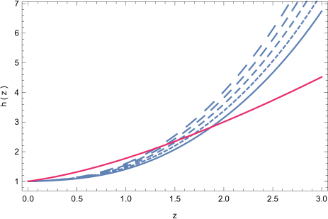
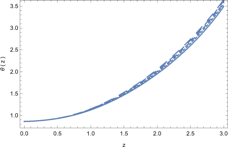
Figure 1: Variation of the dimensionless Hubble function $h$ (left figure) and of the dimensionless vector potential $\theta$ of the dark energy (right figure) as a function of the redshift $z$ in the Einstein dark energy model for $\gamma=1$, $\tilde{k}=0.85$, $\nu=0.50$, and for different values of the parameter $\zeta$: $\zeta=10$ (solid curve), $\zeta=11$ (dotted curve), $\zeta=12$ (short dashed curve), $\zeta=13$ (dashed curve), and $\zeta=14$ (long dashed curve), respectively. The initial conditions used to integrate the field equations (110) and (111) are $h(0)=1$ and $\theta(0)=0.86$. The red curve in the right figure represents the redshift variation of the dimensionless Hubble function in the standard $\Lambda$CDM cosmological model.

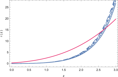
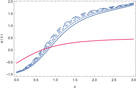
Figure 2: Variation of the dimensionless matter energy density $r$ (left figure) and of the deceleration parameter $q$ of the dark energy (right figure) as a function of the redshift $z$ in the Einstein dark energy model for $\gamma=1$, $\tilde{k}=0.85$, $\nu=0.5$, and for different values of the parameter $\zeta$: $\zeta=10$ (solid curve), $\zeta=11$ (dotted curve), $\zeta=12$ (short dashed curve), $\zeta=13$ (dashed curve), and $\zeta=14$ (long dashed curve), respectively. The initial conditions used to integrate the field equations (110) and (111) are $h(0)=1$ and $\theta(0)=0.86$. The red curves in the figures represent the redshift variation of the dimensionless matter energy density and of the deceleration parameter in the standard $\Lambda$CDM cosmological model.

As one can see from the left panel of Fig. 1, the Hubble function is an increasing function of the redshift (a decreasing function of the cosmological time), indicating an expansionary evolution of the Universe filled with Einstein type dark energy. The evolution of the Hubble function is strongly dependent on the numerical values of the parameter $\zeta$, and small variations of this parameter can induce important modifications in the overall expansion rate of the Universe. In the redshift range $z\in(0,0.2)$ the Hubble function becomes a constant, indicating the presence of a de Sitter type evolution, which is independent on the numerical values of the model parameters. The vector field potential $\theta$, depicted in the right panel of Fig. 1, is also an increasing function of the redshift $z$, indicating a time decreasing evolution of the vector field. The dynamics of $\theta$ is strongly dependent by the considered variations of the model parameters, and this dependence is particularly important at high redshifts. The dimensionless matter energy density, represented in the left panel of Fig. 2, is a monotonically increasing function of the redshift, and its evolution at high redshifts is strongly dependent on the numerical values of the model parameter $\zeta$. But for redshift values in the range $z\in(0,0.2)$, the variation of $r$ is basically independent of the variation of $\zeta$. In this model the energy density of the Universe is generally non-zero at the present time, $r(0)\neq 0$, indicating the possibility of an accelerated evolution in the presence of (very low density) dust matter. The deceleration parameter $q$, plotted in the right panel of Fig. 2, shows a complex behavior. The evolution of the Universe begins at a redshift $z=3$ from a decelerating state, with $q\approx 2$. The numerical values of $q$ decrease in time, and the deceleration parameter reaches its marginally accelerating value $q=0$ at around $z=z_{cr}\approx 0.65-0.80$. For values of $z<z_{cr}$ the Universe enters in an accelerating phase with $q<0$, and reaches a state with $q\approx-1$ at the present time. At high redshifts the evolution of $q$ is dependent on the numerical values of the model parameter $\zeta$. In the redshift range $z\in(0,0.10)$ the evolution of $q$ does not depend essentially on the model parameters. Moreover, the de Sitter type phase, with $q\approx-1$, reached at $z=0$, is an attractor of the gravitational field equations- no matter the initial conditions of the expansion, the Universe always ends in a state with an exponentially increasing scale factor.

It is also interesting to perform a comparison, at a qualitative level, between the evolution of the Einstein dark energy dominated Universe, and the standard $\Lambda$CDM model. The basic difference between the two models is related to the fact that, as one can see from the right panel in Fig. 2, in the Einstein dark energy model at the present time the Universe enters in the exact de Sitter phase, with $q=-1$, while in the $\Lambda$CDM model at the present time $q=-0.53$. This means that in the presence of the Einstein type vector dark energy the Universe accelerates more rapidly, with the de Sitter phase with $q\approx-1$ already reached at $z\approx 0.20$. On the other hand, at least for the considered set of model parameters, the predictions for the numerical values of the deceleration parameter are very different. While the $\Lambda$CDM model gives a value of $q\approx 0.1$ at $z=3$, in the present dark energy model the deceleration parameter has values of the order of $q\approx 2$ at $z=3$. However, this value is strongly dependent on the choice of the model parameters $\nu$, $\tilde{k}$, and $\zeta$, and on the initial value/present day value of the vector field $\theta$. Both models predict the presence of cosmological matter at $z=0$. However, due to the much earlier presence of the de Sitter phase, the matter content of the Universe in the Einstein dark energy model is much more diluted than in the standard $\Lambda$CDM model. The evolution of the Hubble function in the $\Lambda$CDM model is different from its evolution in the Einstein dark energy model at both low and high redshifts. At $z=0$ it is not yet a constant, and at high redshifts it has numerical values around two times smaller as compared to the predictions of the Einstein dark energy model.

VI Discussions and final remarks

In 1919 Einstein proposed an intriguing theory according to which the gravitational interaction plays an essential role at the level of elementary particles. The basic assumption in Einstein’s theory is that material particles are held together by the gravitational force, which such compensates for the presence of the electromagnetic interactions. There are two major results in Einstein’s paper: an explanation of the nature of the cosmological constant, which naturally appears as a ”simple” arbitrary integration constant, and, more intriguingly, that the energy balance of material bodies must consist of 25% gravitational (matter) energy, and 75% of electromagnetic type energy.

We believe that the interest for this model may go beyond its historical importance, the possible explanation of the matter-energy composition of the Universe, and of the possibility of solving (at least partially) the cosmological constant problem. The Einstein model is also very interesting, and important, from a general theoretical point of view, since for the first time it did suggest that matter may play a more important role in the framework of gravitational theories as compared to standard general relativity. In the Einstein geometry-matter symmetric field equations matter appears in a mathematically equivalent form with geometry. Hence in this sense Einstein’s 1919’s theory is a precursor of the present day $f(R,T)$ gravity theories frt1 . On the other hand Einstein’s theory also represents a drastic departure from the standard, and (almost) universally accepted, assumption of the conservation of the matter energy-momentum tensor. Particle creation is also a characteristic feature of quantum field theory in curved space-times bookf , and thus one may interpret non-conservative gravitational models as a first order approximation to quantum gravity phenomenology. The introduction of a coupling between the quantum fields and the curvature of the space-time, as proposed, for example, in Kibble , leads, in the semi-classical approximation, to the non-conservation of the quantum average of the matter energy-momentum tensor operator, so that $\nabla_{\mu}\left<\hat{T}^{\mu\nu}\right>\neq 0$. Thus, theoretical field gravitational models that describe effective particle creation processes can be interpreted as giving a description at an effective semiclassical level of the quantum processes in a gravitational field. Therefore a possible physical explanation of the matter production processes in the Einstein dark energy model may be traced back to the semiclassical approximation of the quantum field theory in a Riemannian curved geometry. On the other hand, if the quantum metric can be decomposed as the sum of the classical and of a fluctuating part, of quantum origin, at the classical level the corresponding Einstein quantum gravitational field equations lead to modified gravity models with a nonminimal coupling between geometry and matter Liu , indicating an irreversible transformation of the quantum energy flow of the gravitational field into a matter fluid. Hence Einstein’s ”theory of elementary particles” may provide some insights into the possibility of the effective description of gravity at quantum level, where the strict distinction between matter and geometry may not exist anymore.

In the present paper we have extended Einstein’s elementary particle model to the scale of the biggest possible particle, the Universe. We have substituted the ”simple” electromagnetic force by a vector type dark energy, and we have generalized the Einstein model by assuming that the vector dark energy is massive, has self-interaction, described by a corresponding potential, and couples with the matter current. Under these assumptions we have formulated the variational principle from which the field equations of the Einstein dark energy model can be obtained. The Einstein field equations from 1919 Ein2 can also be obtained as a limiting case from this variational principle. The initial Einstein theory is non-conservative, and this feature was automatically transferred to its generalization. Non-conservation of matter can be described naturally in the framework of the thermodynamics of open systems as describing matter and entropy creation through the transfer of gravitational energy.

In the present paper we have also investigated in detail the cosmological properties of the Einstein cosmological models. The vector field self-interaction potential was assumed to be of a simple polynomial form, constructed by analogy with the Higgs potential Aad , which plays a fundamental role in theoretical particle physics as describing the generation of mass of the quantum elementary particles.

In the framework of the Einstein dark energy model we have investigated two cosmological evolution scenarios, corresponding to matter conservation, and non-conservation, respectively. In the non-conservative case, in the large time (small redshift) limit, the Universe enters in an accelerating stage, with the exponential de Sitter solution acting as an attractor for these cosmological models. The deceleration parameter reaches the marginal $q=0$ value at a redshift of the order of $z\approx 0.65-0.80$. However, the time evolution of the deceleration parameter strongly depends on the numerical values of the model parameters, describing the mass of the dark energy field, the coupling between dark energy and matter current, and of the functional form of the self-interaction potential $V$. In order to obtain a better understanding on the numerical values of these parameters the fitting of the model with the cosmological observational data should be performed. This in depth comparison of the theoretical predictions with the observational data can give the answer to the question if Einstein did really predict almost 100 years ago the correct ”chemical and energy composition” of the Universe.

Hopefully the Einstein dark energy model introduced in the present paper could give some new insights into the complex problem of the evolutionary dynamics, composition and structure of the Universe, from its birth to the latest stages of evolution.

References

- (1) A. Einstein, Sitzungsberichte der Königlich Preussischen Akademie der Wissenschaften (Berlin), part 1, 142 (1917).
- (2) A. Einstein, Sitzungsberichte der Königlich Preussischen Akademie der Wissenschaften (Berlin), 349 (1919).
- (3) W. Pauli, Theory of Relativity, Pergamon Press, London, New York, Paris, Los Angeles, 1958
- (4) F. Jüttner, Math. Ann. 87, 270 (1922).
- (5) S. Weinberg, Reviews of Modern Physics 61, 1 (1989).
- (6) P. Rastall, Phys. Rev. D 6, 3357 (1972).
- (7) C. E. M. Batista, M. H. Daouda, J. C. Fabris, O. F. Piattella, and D. C. Rodrigues, Phys. Rev. D 85, 084008 (2012).
- (8) J. C. Fabris, M. Hamani Daouda, and O. F. Piattella, Physics Letters B 711, 232 (2012).
- (9) C. E. M. Batista, J. C. Fabris, O. F. Piattella, and A. M. Velasquez-Toribio, Eur. Phys. J. C 73, 2425 (2013).
- (10) J. P. Campos, J. C. Fabris, R. Perez, O. F. Piattella, and H. Velten, Eur. Phys. J. C 73, 2357 (2013).
- (11) T. R. P. Carams, M. H. Daouda, J. C. Fabris, A. M. de Oliveira, O. F. Piattella, and V. Strokov, Eur. Phys. J. C 74, 3145 (2014).
- (12) A. M. Oliveira, H. E. S. Velten, J. C. Fabris, and L. Casarini, Phys. Rev. D 92, 044020 (2015).
- (13) H. Moradpour, Phys. Lett. B 757, 187 (2016).
- (14) A. M. Oliveira, H. E. S. Velten, and J. C. Fabris, Phys. Rev. D 93, 124020 (2016).
- (15) Y. Heydarzade and F. Darabi, arXiv:1702.07766 [gr-qc].
- (16) F.-F. Yuan and P. Huang, Class. Quant Grav. 34, 077001 (2017).
- (17) H. Moradpour, Y. Heydarzade, F. Darabi, and I. G. Salako, Eur. Phys. J. C 77, 259 (2017).
- (18) R. Vieira dos Santos and J. A. C. Nogales, arXiv:1701.08203 [gr-qc].
- (19) T. Harko, F. S. N. Lobo, S. Nojiri, and S. D. Odintsov, Phys. Rev. D 84, 024020 (2011).
- (20) M. Sharif and M. Zubair, JCAP 03, 028 (2012).
- (21) M. Jamil, D. Momeni, M. Raza, and R. Myrzakulov, Eur. Phys. J. C 72, 1999 (2012).
- (22) F. G. Alvarenga, A. de la Cruz-Dombriz, M. J. S. Houndjo, M. E. Rodrigues, and D. Saez-Gomez, Phys. Rev. D 87, 103526 (2013).
- (23) H. Shabani and M. Farhoudi, Phys. Rev. D 88, 044048 (2013).
- (24) O. J. Barrientos and G. F. Rubilar, Phys. Rev. D 90, 028501 (2014).
- (25) H. Shabani and M. Farhoudi, Phys. Rev. D 90, 044031 (2014).
- (26) I. Noureen and M. Zubair, Eur. Phys. J. C 75, 62 (2015).
- (27) M. Zubair and I. Noureen, Eur. Phys. J. C 75, 265 (2015).
- (28) I. Noureen, M. Zubair, A. A. Bhatti, and G. Abbas, Eur. Phys. J. C 75, 323 (2015).
- (29) M.-X. Xu, T. Harko, and S.-D. Liang, Eur. Phys. J. C 76, 1 (2016).
- (30) H. Shabani and A. H. Ziaie, Eur. Phys. J. C 77, 282 (2017).
- (31) O. Bertolami, C. G. Boehmer, T. Harko, and F. S. N. Lobo, Phys. Rev. D 75, 104016 (2007).
- (32) T. Harko, Phys. Lett. B 669, 376 (2008).
- (33) T. Harko and F. S. N. Lobo, Eur. Phys. J. C 70, 373 (2010).
- (34) T. Harko, F. S. N. Lobo, and O. Minazzoli, Phys. Rev. D 87, 047501 (2013).
- (35) Z. Haghani, T. Harko, H. R. Sepangi, and S. Shahidi, JCAP 10, 061 (2012); Z. Haghani, T. Harko, H. R. Sepangi, and S. Shahidi, Phys. Rev. D 88, 044024 (2013).
- (36) Z. Haghani, N. Khosravi and S. Shahidi, Class. Quant Grav. 32, 215016 (2015).
- (37) T. Harko, T. S. Koivisto, F. S. N. Lobo, and G. J. Olmo, Phys. Rev. D 85, 084016 (2012).
- (38) N. Tamanini and C. G. Böhmer, Phys. Rev. D 87, 084031 (2013).
- (39) S. Capozziello, T. Harko, T. S. Koivisto, F. S. N. Lobo, and G. J. Olmo, Universe 1, 199 (2015).
- (40) Z. Haghani, T. Harko, F. S. N. Lobo, H. R. Sepangi, and S. Shahidi, Phys. Rev. D 88, 044023 (2013).
- (41) S. D. Odintsov and D. Saez-Gomez, Phys. Lett. B 725, 437 (2013).
- (42) T. Harko, F. S. N. Lobo, G. Otalora, and E. N. Saridakis, JCAP 12, 021 (2014).
- (43) T. Clifton, P. G. Ferreira, A. Padilla, and C. Skordis, Phys. Repts. 513, 1 (2012).
- (44) A. G. Riess et al., Astron. J. 116, 1009 (1998).
- (45) S. Perlmutter et al., Astrophys. J. 517, 565 (1999).
- (46) R. A. Knop et al., Astrophys. J. 598, 102 (2003).
- (47) R. Amanullah et al., Astrophys. J. 716, 712 (2010).
- (48) M. Bojowald, Rep. Prog. Phys. 78, 023901 (2015).
- (49) D. Battefeld and P. Peter, Physics Reports 571, 1 (2015).
- (50) M. Kilbinger, Rep. Prog. Phys. 78, 086901 (2015).
- (51) I. Antoniadis and S. Cotsakis, Int. J. Mod. Phys. D 26, 1730009 (2017).
- (52) N. J. Nunes, P. Martin-Moruno, and F. S. N. Lobo, Universe 3, 33 (2017).
- (53) P. J. E. Peebles and B. Ratra, Rev. Mod. Phys. 75, 559 (2003).
- (54) T. Padmanabhan, Phys. Repts. 380, 235 (2003).
- (55) E. V. Linder, Rept. Prog. Phys. 71, 056901 (2008).
- (56) A. Silvestri and M. Trodden, Rept. Prog. Phys. 72, 096901 (2009).
- (57) A. Joyce, B. Jain, J. Khoury, and M.Trodden, Phys. Rept. 568, 1 (2015).
- (58) D. H. Weinberg, M. J. Mortonson, D. J. Eisenstein, C. Hirata, A. G. Riess, and E. Rozo, Physics Reports 530, 87 (2013).
- (59) S. Hee, J.A. Vázquez, W. J. Handley, M. P. Hobson, and A. N. Lasenby, Month. Not. R. Atron. Soc 466, 369 (2016).
- (60) A. Tripathi, A. Sangwan, and H. K. Jassal, JCAP 06, 012 (2017).
- (61) D. Wang and X.-H. Meng, Phys. Rev. D 95, 023508 (2017).
- (62) J.-P. Dai, Y. Yang, and J.-Q. Xia, Astrophys. J. 857, 9 (2018).
- (63) P. A. R. Ade et al., Planck collaboration, Planck 2015 results. XIII. Cosmological parameters, Astron. Astrophys. 594, A13 (2016).
- (64) R. Caldwell, R. Dave and P. J. Steinhardt, Phys. Rev. Lett. 80, 1582 (1998).
- (65) S. Tsujikawa, Class. Quant. Grav. 30, 214003 (2013).
- (66) T. Harko and F. S. N. Lobo, Phys. Rev. D 87, 044018 (2013).
- (67) T. Harko and F. S. N. Lobo, JCAP 1307, 036 (2013).
- (68) A. Nicolis, R. Rattazzi, and E. Trincherini, Phys. Rev. D 79, 064036 (2009).
- (69) C. Defayet, G. Esposito-Farese and A. Vikman, Phys. Rev. D 79, 084003 (2009).
- (70) C. de Rham and A. J. Tolley, JCAP 1005, 015 (2010).
- (71) G. Goon, K. Hinterbichler and M. Trodden, Phys. Rev. Lett. 106, 231102 (2011).
- (72) K. Kamada, T. Kobayashi, M. Yamaguchi and J. I. Yokoyama, Phys. Rev. D 83, 083515 (2011).
- (73) T. Kobayashi, M. Yamaguchi and J. I. Yokoyama, Prog. Theor. Phys. 126, 511 (2011).
- (74) A. De Felice, S. Tsujikawa, Phys. Rev. Lett. 105, 111301 (2010); A. De Felice and S. Tsujikawa, JCAP 1203, 025 (2012); M. Shahalam, S. K. J. Pacif and R. Myrzakulov, Eur. Phys. J. C 76, 410 (2016).
- (75) V. A. Rubakov, arXiv:1401.4024.
- (76) R. R. Caldwell, Phys. Lett. B. 545, 23 (2002).
- (77) S. M. Carroll, M. Hoffman, and M. Trodden, Phys. Rev. D 68, 023509 (2003).
- (78) P. Singh, M. Sami, and N. Dadhich, Phys. Rev. D 68, 023522 (2003).
- (79) J. M. Cline, S. Jeon, and G. D. Moore, Phys. Rev. D 70, 043543 (2004).
- (80) E. Elizalde, S. Nojiri, S. D. Odintsov, D. Saez-Gomez and V. Faraoni, Phys. Rev. D 77, 106005 (2008).
- (81) A. Yu. Kamenshchik, Class. Quantum Grav. 30, 173001 (2013).
- (82) U. Alam, V. Sahni, T. D. Saini, and A. A. Starobinsky, Mon. Not. Roy. Astron. Soc. 354, 275 (2004).
- (83) C. Armendariz-Picon, J. Cosmol. Astropart. Phys. 07 (2004) 007.
- (84) H. Wei and R.-G. Cai, Phys. Rev. D 73, 083002 (2006).
- (85) T. S. Koivisto and D. F. Mota, JCAP 0808, 021 (2008).
- (86) J. B. Jimenez and A. L. Maroto, Phys. Rev. D 78, 063005 (2008).
- (87) J. B. Jimenez, R. Lazkoz, and A. L. Maroto, Phys. Rev. D 80, 023004 (2009).
- (88) E. Carlesi, A. Knebe, G. Yepes, S. Gottloeber, J. Beltrán Jiménez, and A. L. Maroto, Monthly Not. Royal Astron. Soc. 418, 2715 (2011).
- (89) E. Carlesi, A. Knebe, G. Yepes, S. Gottloeber, J. B. Jimenez, and A. L. Maroto, Month. Not. R. Astron. Soc. 418, 2715 (2011).
- (90) E. Carlesi, A. Knebe, G. Yepes, S. Gottloeber, J. Beltrán Jiménez, A. L. Maroto, Monthly Not. Royal Astron. Soc. 424, 699 (2012).
- (91) M. Chaichian, J. Kluson, M. Oksanen, and A. Tureanu, JHEP 12, 102 (2014).
- (92) R. Dale and D. Sáez, Phys. Rev. D 89, 044035 (2014).
- (93) R. C. G. Landim, Eur. Phys. J. C 76, 480 (2016).
- (94) J. J. Beltran and T. Koivisto, Universe 3, 47 (2017).
- (95) R. Dale and D. Sáez, JCAP 01, 004 (2017).
- (96) S. Jamali, M. Roshan, and L. Amendola, JCAP 01, 048 (2018).
- (97) C. G. Böhmer and T. Harko, Eur. Phys. J. C 50, 423 (2007).
- (98) G. Esposito-Farese, C. Pitrou, and J.-P. Uzan, Phys. Rev. D81, 063519 (2010).
- (99) J. B. Jiménez, A. L. Delvas Fróes, and D. F. Mota, Phys. Lett. B 725, 212 (2013).
- (100) S. Kouwn, P. Oh, and C.-G. Park, Phys. Rev. D 93, 083012 (2016).
- (101) F. Tamburini, M. De Laurentis, L. Amati, and B. Thidé, Phys. Rev. D 96, 104003 (2017).
- (102) Z. Haghani, T. Harko, H. R. Sepangi, and S. Shahidi, Eur. Phys. Journal C 77 137 (2017).
- (103) Z. Haghani, T. Harko, and S. Shahidi, Eur. Phys. J. C 77, 514 (2017).
- (104) S.-D. Liang and T. Harko, Phys. Rev. D 91, 085042 (2015).
- (105) Z. Keresztes, L. A. Gergely, T. Harko, and S.-D. Liang, Phys. Rev. D 92, 123503 (2015).
- (106) L. D. Landau and E. M. Lifshitz, The classical theory of fields, Oxford, Pergamon Press, United Kingdom, 1971.
- (107) I. Prigogine and J. Géhéniau, Proc. Natl. Acad. Sci. USA 83, 6245 (1986).
- (108) I. Prigogine, J. Géhéniau, E. Gunzig, and P. Nardone, Proc. Natl. Acad. Sci. USA 85, 7428 (1988).
- (109) M. O. Calvo, J. A. S. Lima, and I. Waga, Phys.lett. A 162, 223 (1992).
- (110) J. A. S. Lima and A. S. M. Germano, Phys. Lett. A 170, 373 (1992).
- (111) T. Harko, Phys. Rev. D 90, 044067 (2014).
- (112) T. Harko, F. S. N. Lobo, J. P. Mimoso, and D. Pavón, Eur. Phys. J. C 75, 386 (2015).
- (113) S. Weinberg, Astrophys. J. 168, 175 (1971).
- (114) L. E. Parker and D. J. Toms, Quantum Field Theory in Curved Spacetime-Quantized Fields and Gravity, Cambridge, Cambridge University Press, 2009.
- (115) T. W. B. Kibble and S. Randjbar-Daemi, J. Phys. A: Math. Gen. 13, 141 (1980).
- (116) X. Liu, T. Harko, and S.-D. Liang, Eur. Phys. J. C 76, 420 (2016).
- (117) G. Aad et al., Phys. Rev. Lett. 115, 131801 (2015).