Hook formulas for skew shapes III. Multivariate
and product formulas

Alejandro H. Morales,   Igor Pak,  and   Greta Panova
Abstract.

We give new product formulas for the number of standard Young tableaux of certain skew shapes and for the principal evaluation of certain Schubert polynomials. These are proved by utilizing symmetries for evaluations of factorial Schur functions, extensively studied in the first two papers in the series [MPP1, MPP2]. We also apply our technology to obtain determinantal and product formulas for the partition function of certain weighted lozenge tilings, and give various probabilistic and asymptotic applications.

Department of Mathematics and Statistics, UMass Amhest, Amherst, MA 01003. Email: ahmorales@math.umass.edu
Department of Mathematics, UCLA, Los Angeles, CA 90095.  Email: pak@math.ucla.edu
Department of Mathematics, USC, Los Angeles, CA, 90089.  Email: gpanova@usc.edu

1. Introduction

1.1. Foreword

It is a truth universally acknowledged, that a combinatorial theory is often judged not by its intrinsic beauty but by the examples and applications. Fair or not, this attitude is historically grounded and generally accepted. While eternally challenging, this helps to keep the area lively, widely accessible, and growing in unexpected directions.

There are two notable types of examples and applications one can think of:  artistic  and  scientific  (cf. [Gow]). The former are unexpected results in the area which are both beautiful and mysterious. The fact of their discovery is the main application, even if they can be later shown by a more direct argument. The latter are results which represent a definitive progress in the area, unattainable by other means. To paraphrase Struik, this is “something to take home”, rather than to simply admire (see [Rota]). While the line is often blurred, examples of both types are highly desirable, with the best examples being both artistic and scientific.

This paper is a third in a series and continues our study of the Naruse hook-length formula (NHLF), its generalizations and applications. In the first paper [MPP1], we introduced two q𝑞q-analogues of the NHLF and gave their (difficult) bijective proofs. In the second paper [MPP2], we investigated the special case of ribbon hooks, which were used to obtain two new elementary proofs of NHLF in full generality, as well as various new mysterious summation and determinant formulas.

In this paper we present three new families of examples and applications of our tools:

\bullet  new product formulas for the number of standard Young tableaux of certain skew shapes,

\bullet  new product formulas for the principal evaluation of certain Schubert polynomials,

\bullet  new determinantal formulas for weighted enumeration of lozenge tilings of a hexagon.

All three directions are so extensively studied from enumerative point of view, it is hard to imagine there is room for progress. In all three cases, we generalize a number of existing results within the same general framework of factorial Schur functions. With one notable exception (see §§\S9.4), we cannot imagine a direct combinatorial proof of the new product formulas circumventing our reasoning (cf. §§\S9.2, however). As an immediate consequence of our results, we obtain exact asymptotic formulas which were unreachable until now (see sections 6 and 8). Below we illustrate our results one by one, leaving full statements and generalizations for later.

1.2. Number of SYT of skew shape

Standard Young tableaux are fundamental objects in enumerative and algebraic combinatorics and their enumeration is central to the area (see e.g. [Sag2, Sta1]). The number  fλ=|SYT(λ)|superscript𝑓𝜆SYT𝜆f^{\lambda}=\bigl{|}\operatorname{{\rm SYT}}(\lambda)\bigr{|}  of standard Young tableaux of shape λ𝜆\lambda and size n𝑛n, is given by the classical hook-length formula:

(HLF) fλ=n!u[λ]1h(u).superscript𝑓𝜆𝑛subscriptproduct𝑢delimited-[]𝜆1𝑢f^{\lambda}\,=\,n!\,\prod_{u\in[\lambda]}\frac{1}{h(u)}\hskip 1.70709pt.

Famously, there is no general product formula for the number  fλ/μ=|SYT(λ/μ)|superscript𝑓𝜆𝜇SYT𝜆𝜇f^{\lambda/\mu}=\bigl{|}\operatorname{{\rm SYT}}(\lambda/\mu)\bigr{|}  of standard Young tableaux of skew shape λ/μ𝜆𝜇\lambda/\mu.111In fact, even for small zigzag shapes π=δk+2/δk𝜋subscript𝛿𝑘2subscript𝛿𝑘\pi=\delta_{k+2}/\delta_{k}, ¡ the number fπsuperscript𝑓𝜋f^{\pi} can have large prime divisors (cf. §§\S5.3). However, such formulas do exist for a few sporadic families of skew shapes and truncated shapes (see [AdR]).

In this paper we give a six-parameter family of skew shapes λ/μ=Λ(a,b,c,d,e,m)𝜆𝜇Λ𝑎𝑏𝑐𝑑𝑒𝑚\lambda/\mu=\Lambda(a,b,c,d,e,m) where μ=ba𝜇superscript𝑏𝑎\mu=b^{a} with product formulas for the number of their SYT. The product formulas for these shapes of size n𝑛n include the MacMahon box formula and hook-lengths of certain cells of λ𝜆\lambda:

(1.1) fλ/μ=n!i=1aj=1bk=1ci+j+k1i+j+k2(i,j)λ/0cba1hλ(i,j),superscript𝑓𝜆𝜇𝑛superscriptsubscriptproduct𝑖1𝑎superscriptsubscriptproduct𝑗1𝑏superscriptsubscriptproduct𝑘1𝑐𝑖𝑗𝑘1𝑖𝑗𝑘2subscriptproduct𝑖𝑗𝜆superscript0𝑐superscript𝑏𝑎1subscript𝜆𝑖𝑗f^{\lambda/\mu}\,=\,n!\cdot\prod_{i=1}^{a}\prod_{j=1}^{b}\prod_{k=1}^{c}\hskip 1.70709pt\frac{i+j+k-1}{i+j+k-2}\cdot\,\prod_{(i,j)\in\lambda/0^{c}b^{a}}\,\frac{1}{h_{\lambda}(i,j)}\,,

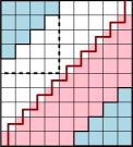
(see Theorem 4.1 and Figure 5 for an illustration of the skew shape and the cells of λ𝜆\lambda whose hook-lengths appear above). The three corollaries below showcase the most elegant special cases. We single out two especially interesting special cases:  Corollary 1.1 due to its connection to the Selberg integral, and Corollary 1.2 due to its relation to shifted shapes and a potential for a bijective proof (see §§\S9.4). These two special cases were known before, but the corresponding proofs do not generalize to the setting of this paper.

The formulas below are written in terms of superfactorials Φ(n)Φ𝑛\Phi(n), double superfactorials (n)𝑛\gimel(n), super doublefactorials Ψ(n)Ψ𝑛\Psi(n), and shifted super doublefactorials Ψ(n;k)Ψ𝑛𝑘\Psi(n;k) defined as follows:

Φ(n)Φ𝑛\displaystyle\Phi(n) :=1!2!(n1)!,(n):=(n2)!(n4)!,formulae-sequenceassignabsent12𝑛1assign𝑛𝑛2𝑛4\displaystyle:=\hskip 1.70709pt1!\cdot 2!\hskip 0.85355pt\cdots\hskip 0.85355pt(n-1)!\,,\qquad\quad\hskip 1.70709pt\hskip 1.70709pt\gimel(n)\hskip 1.70709pt:=\hskip 1.70709pt(n-2)!(n-4)!\hskip 0.85355pt\cdots\hskip 1.70709pt,
Ψ(n)Ψ𝑛\displaystyle\Psi(n) :=1!!3!!(2n3)!!,Ψ(n;k):=(k+1)!!(k+3)!!(k+2n3)!!formulae-sequenceassignabsentdouble-factorial1double-factorial3double-factorial2𝑛3assignΨ𝑛𝑘double-factorial𝑘1double-factorial𝑘3double-factorial𝑘2𝑛3\displaystyle:=\hskip 1.70709pt1!!\cdot 3!!\hskip 0.85355pt\cdots\hskip 0.85355pt(2n-3)!!\,,\qquad\Psi(n;k)\hskip 1.70709pt:=\hskip 1.70709pt(k+1)!!\hskip 0.85355pt\cdots\hskip 0.85355pt(k+3)!!\hskip 0.85355pt\cdots\hskip 0.85355pt(k+2n-3)!!
Corollary 1.1 (Kim–Oh [KO1], see §9.3).

For all  a,b,c,d,e𝑎𝑏𝑐𝑑𝑒a,b,c,d,e\in\mathbb{N}, let λ/μ𝜆𝜇\lambda/\mu be the skew shape in  Figure 1 (i). Then the number  fλ/μ=|SYT(λ/μ)|superscript𝑓𝜆𝜇SYT𝜆𝜇f^{\lambda/\mu}=\bigl{|}\operatorname{{\rm SYT}}(\lambda/\mu)\bigr{|}  is equal to

n!Φ(a)Φ(b)Φ(c)Φ(d)Φ(e)Φ(a+b+c)Φ(c+d+e)Φ(a+b+c+d+e)Φ(a+b)Φ(d+e)Φ(a+c+d)Φ(b+c+e)Φ(a+b+2c+d+e),𝑛Φ𝑎Φ𝑏Φ𝑐Φ𝑑Φ𝑒Φ𝑎𝑏𝑐Φ𝑐𝑑𝑒Φ𝑎𝑏𝑐𝑑𝑒Φ𝑎𝑏Φ𝑑𝑒Φ𝑎𝑐𝑑Φ𝑏𝑐𝑒Φ𝑎𝑏2𝑐𝑑𝑒n!\,\hskip 1.70709pt\frac{\Phi(a)\hskip 1.70709pt\Phi(b)\hskip 1.70709pt\Phi(c)\hskip 1.70709pt\Phi(d)\hskip 1.70709pt\Phi(e)\hskip 1.70709pt\Phi(a+b+c)\hskip 1.70709pt\Phi(c+d+e)\hskip 1.70709pt\Phi(a+b+c+d+e)}{\Phi(a+b)\hskip 1.70709pt\Phi(d+e)\hskip 1.70709pt\Phi(a+c+d)\hskip 1.70709pt\Phi(b+c+e)\hskip 1.70709pt\Phi(a+b+2c+d+e)}\,,

where n=|λ/μ|=(a+c+e)(b+c+d)abed𝑛𝜆𝜇𝑎𝑐𝑒𝑏𝑐𝑑𝑎𝑏𝑒𝑑n=|\lambda/\mu|=(a+c+e)(b+c+d)-ab-ed.

Note that in [KO1, Cor. 4.7], the product formula is equivalent, but stated differently.

Corollary 1.2 (DeWitt [DeW], see §9.4).

For all  a,b,c𝑎𝑏𝑐a,b,c\in\mathbb{N}, let λ/μ𝜆𝜇\lambda/\mu be the skew shape in  Figure 1 (ii). Then the number  fλ/μ=|SYT(λ/μ)|superscript𝑓𝜆𝜇SYT𝜆𝜇f^{\lambda/\mu}=\bigl{|}\operatorname{{\rm SYT}}(\lambda/\mu)\bigr{|}  is equal to

n!Φ(a)Φ(b)Φ(c)Φ(a+b+c)Ψ(c)Ψ(a+b+c)Φ(a+b)Φ(b+c)Φ(a+c)Ψ(a+c)Ψ(b+c)Ψ(a+b+2c),𝑛Φ𝑎Φ𝑏Φ𝑐Φ𝑎𝑏𝑐Ψ𝑐Ψ𝑎𝑏𝑐Φ𝑎𝑏Φ𝑏𝑐Φ𝑎𝑐Ψ𝑎𝑐Ψ𝑏𝑐Ψ𝑎𝑏2𝑐n!\,\,\frac{\Phi(a)\hskip 1.70709pt\Phi(b)\hskip 1.70709pt\Phi(c)\hskip 1.70709pt\Phi(a+b+c)\hskip 0.85355pt\cdot\hskip 0.85355pt\Psi(c)\hskip 1.70709pt\Psi(a+b+c)}{\Phi(a+b)\hskip 1.70709pt\Phi(b+c)\hskip 1.70709pt\Phi(a+c)\hskip 0.85355pt\cdot\hskip 0.85355pt\Psi(a+c)\hskip 1.70709pt\Psi(b+c)\hskip 1.70709pt\Psi(a+b+2c)}\,,

where n=|λ/μ|=(a+b+2c2)ab𝑛𝜆𝜇binomial𝑎𝑏2𝑐2𝑎𝑏n=|\lambda/\mu|=\binom{a+b+2c}{2}-ab.

Refer to caption
Figure 1. Skew shapes Λ(a,b,c,d,e,0)Λ𝑎𝑏𝑐𝑑𝑒0\Lambda(a,b,c,d,e,0), Λ(a,b,c,0,0,1)Λ𝑎𝑏𝑐001\Lambda(a,b,c,0,0,1) and Λ(a,b,c,d,e,1)Λ𝑎𝑏𝑐𝑑𝑒1\Lambda(a,b,c,d,e,1) with product formulas for the number of SYT.
Corollary 1.3.

For all  a,b,c,d,e𝑎𝑏𝑐𝑑𝑒a,b,c,d,e\in\mathbb{N}, let λ/μ𝜆𝜇\lambda/\mu be the skew shape in  Figure 1 (iii). Then the number  fλ/μ=|SYT(λ/μ)|superscript𝑓𝜆𝜇SYT𝜆𝜇f^{\lambda/\mu}=\bigl{|}\operatorname{{\rm SYT}}(\lambda/\mu)\bigr{|}  is equal to

n!Φ(a)Φ(b)Φ(c)Φ(a+b+c)Ψ(c;d+e)Ψ(a+b+c;d+e)(d)(e)(2a+2c)(2b+2c)Φ(a+b)Φ(b+c)Φ(a+c)Ψ(a+c)Ψ(b+c)Ψ(a+b+2c;d+e)(2a+2c+d)(2b+2c+e),𝑛Φ𝑎Φ𝑏Φ𝑐Φ𝑎𝑏𝑐Ψ𝑐𝑑𝑒Ψ𝑎𝑏𝑐𝑑𝑒𝑑𝑒2𝑎2𝑐2𝑏2𝑐Φ𝑎𝑏Φ𝑏𝑐Φ𝑎𝑐Ψ𝑎𝑐Ψ𝑏𝑐Ψ𝑎𝑏2𝑐𝑑𝑒2𝑎2𝑐𝑑2𝑏2𝑐𝑒\frac{n!\hskip 1.70709pt\cdot\hskip 1.70709pt\Phi(a)\hskip 0.85355pt\Phi(b)\hskip 0.85355pt\Phi(c)\hskip 0.85355pt\Phi(a+b+c)\hskip 0.85355pt\cdot\hskip 0.85355pt\Psi(c;d+e)\hskip 0.85355pt\Psi(a+b+c;d+e)\hskip 0.85355pt\cdot\hskip 0.85355pt\gimel(d)\hskip 0.85355pt\gimel(e)\hskip 0.85355pt\gimel(2a+2c)\hskip 0.85355pt\gimel(2b+2c)}{\Phi(a+b)\hskip 0.85355pt\Phi(b+c)\hskip 0.85355pt\Phi(a+c)\cdot\Psi(a+c)\hskip 0.85355pt\Psi(b+c)\hskip 0.85355pt\Psi(a+b+2c;d+e)\cdot\gimel(2a+2c+d)\hskip 0.85355pt\gimel(2b+2c+e)}\,,

where n=|λ/μ|=(a+c+e)(b+c+d)+(a+c2)+(b+c2)abed𝑛𝜆𝜇𝑎𝑐𝑒𝑏𝑐𝑑binomial𝑎𝑐2binomial𝑏𝑐2𝑎𝑏𝑒𝑑\hskip 0.85355ptn=|\lambda/\mu|=(a+c+e)(b+c+d)+\binom{a+c}{2}+\binom{b+c}{2}-ab-ed.

Let us emphasize that the proofs of corollaries 1.11.3 are quite technical in nature. Here is a brief non-technical explanation. Fundamentally, the Naruse hook-length formula (NHLF) provides a new way to understand SYT of skew shape, coming from geometry rather than representation theory. What we show in this paper is that the proof of the NHLF has “hidden symmetries” which can be turned into product formulas (cf. §§\S9.2). We refer to Section 4 for the complete proofs and common generalizations of these results, including q𝑞q-analogues of the corollaries.

1.3. Product formulas for principal evaluations of Schubert polynomials

The Schubert polynomials𝔖w[x1,,xn1]subscript𝔖𝑤subscript𝑥1subscript𝑥𝑛1\mathfrak{S}_{w}\in\mathbb{Z}[x_{1},\ldots,x_{n-1}], wSn𝑤subscript𝑆𝑛w\in S_{n}, are generalizations of the Schur polynomials and play a key role in the geometry of flag varieties (see e.g. [Mac, Man]). They can be expressed in terms of reduced words (factorizations) of the permutation w𝑤w via the Macdonald identity (2.6), and have been an object of intense study in the past several decades. In this paper we obtain several new product formulas for the principal evaluation𝔖w(1,,1)subscript𝔖𝑤11\mathfrak{S}_{w}(1,\ldots,1)  which has been extensively studied in recent years (see e.g. [BHY, MeS, SeS, Sta4, Wei, Woo]). Below we present two such formulas:

Corollary 1.4 (= Corollary 5.11).

For the permutation  w(a,c):=1c×(24131a)assign𝑤𝑎𝑐superscript1𝑐tensor-product2413superscript1𝑎w(a,c):=1^{c}\times(2413\otimes 1^{a}), where ca𝑐𝑎c\geq a, we have:

𝔖w(a,c)(1,1,,1)=Φ(4a+c)Φ(c)Φ(a)4Φ(3a)2Φ(3a+c)Φ(a+c)Φ(2a)2Φ(4a).subscript𝔖𝑤𝑎𝑐111Φ4𝑎𝑐Φ𝑐Φsuperscript𝑎4Φsuperscript3𝑎2Φ3𝑎𝑐Φ𝑎𝑐Φsuperscript2𝑎2Φ4𝑎\mathfrak{S}_{w(a,c)}(1,1,\ldots,1)\,=\,\frac{\Phi(4a+c)\hskip 1.70709pt\Phi(c)\hskip 1.70709pt\Phi(a)^{4}\hskip 1.70709pt\Phi(3a)^{2}}{\Phi(3a+c)\hskip 1.70709pt\Phi(a+c)\hskip 1.70709pt\Phi(2a)^{2}\hskip 1.70709pt\Phi(4a)}\,.

Here σ×ω𝜎𝜔\sigma\times\omega and σωtensor-product𝜎𝜔\sigma\otimes\omega are the direct sum and the Kronecker product of permutations σ𝜎\sigma and ω𝜔\omega (see §§\S2.2). We denote by by 1nsuperscript1𝑛1^{n} the identity permutation in Snsubscript𝑆𝑛S_{n}.

Corollary 1.5 (= Corollary 5.16).

For the permutation  s(a):=3516241aassign𝑠𝑎tensor-product351624superscript1𝑎s(a):=351624\otimes 1^{a}, we have:

𝔖s(a)(1,1,,1)=Φ(a)5Φ(3a)2Φ(5a)Φ(2a)4Φ(4a)2.subscript𝔖𝑠𝑎111Φsuperscript𝑎5Φsuperscript3𝑎2Φ5𝑎Φsuperscript2𝑎4Φsuperscript4𝑎2\mathfrak{S}_{s(a)}(1,1,\ldots,1)\,=\,\frac{\Phi(a)^{5}\hskip 1.70709pt\Phi(3a)^{2}\hskip 1.70709pt\Phi(5a)}{\Phi(2a)^{4}\hskip 1.70709pt\Phi(4a)^{2}}\,.

These results follow from two interrelated connections between principal evaluations of Schubert polynomials and the number of SYT of skew shapes. Below we give a brief outline, which is somewhat technical (see Section 2 for definitions and details).

The first connection is in the case of vexillary (214321432143-avoiding) permutations. The excited diagrams first appeared in a related context in work of Wachs [Wac] and Knutson–Miller–Yong [KMY], where they gave an explicit formula for the double Schubert polynomials of vexillary permutations in terms of excited diagrams (see §§\S2.5) of a skew shape associated to the permutation. As a corollary, the principal evaluation gives the number of excited diagrams of the skew shape (Theorem 5.4). Certain families of vexillary permutations have skew shapes with product formulas for the number of excited diagrams (see above). Corollary 1.4 is one such example.

The second connection is in the case of 321321321-avoiding permutations. Combining the Macdonald identity and the results of Billey–Jockusch–Stanley [BJS], we show that the principal evaluation for 321321321-avoiding permutations is a multiple of fλ/μsuperscript𝑓𝜆𝜇f^{\lambda/\mu} for a skew shape associated to the permutation (Theorem 5.13). In fact, every skew shape can be realized via a 321321321-avoiding permutation, see [BJS]. In particular, permutations corresponding to the skew shapes in §§\S1.2 have product formulas for the principal evaluations. Corollary 1.5 follows along these lines from Corollary 1.1 with a=b=c=d=e𝑎𝑏𝑐𝑑𝑒a=b=c=d=e.

1.4. Determinantal formulas for lozenge tilings

Lozenge tilings have been studied extensively in statistical mechanics and integrable probability, as exactly solvable dimer models on the hexagonal grid. When the tilings are chosen uniformly at random on a given domain and the mesh size 0absent0\to 0, they have exhibited remarkable limit behavior like limit shape, frozen boundary, Gaussian Unitary Ensemble eigenvalue distributions, Gaussian Free Field fluctuations, etc. Such tilings are studied via a variety of methods ranging from variational principles (see e.g. [CLP, Ken2, KO]), to asymptotics of Schur functions and determinantal processes (see e.g. [BGR, GP, Pet]).

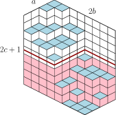
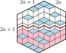
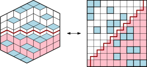
Lozenge tilings of hexagonal shapes correspond naturally to plane partitions, when the lozenges are interpreted as sides of cubes and the tiling is interpreted as a projection of a stack of boxes. For example, lozenge tilings of the hexagon

H(a,b,c):=a×b×c×a×b×cassignH𝑎𝑏𝑐delimited-⟨⟩𝑎𝑏𝑐𝑎𝑏𝑐\operatorname{H}(a,b,c)\hskip 1.70709pt:=\hskip 1.70709pt\langle\hskip 0.85355pta\times b\times c\times a\times b\times c\hskip 0.85355pt\rangle

are in bijection with solid partitions which fit inside the  [a×b×c]delimited-[]𝑎𝑏𝑐[a\times b\times c]  box. Thus, they are counted by the MacMahon box formula, see §§\S2.3 :

(1.2) |PP(a,b,c)|=Φ(a+b+c)Φ(a)Φ(b)Φ(c)Φ(a+b)Φ(b+c)Φ(a+c).PP𝑎𝑏𝑐Φ𝑎𝑏𝑐Φ𝑎Φ𝑏Φ𝑐Φ𝑎𝑏Φ𝑏𝑐Φ𝑎𝑐\bigl{|}\operatorname{PP}(a,b,c)\bigr{|}\,=\,\frac{\Phi(a+b+c)\hskip 1.70709pt\Phi(a)\hskip 1.70709pt\Phi(b)\hskip 1.70709pt\Phi(c)}{\Phi(a+b)\hskip 1.70709pt\Phi(b+c)\hskip 1.70709pt\Phi(a+c)}\,.

This connection allows us to translate our earlier results into the language of weighted lozenge tilings with multivariate weights on horizontal lozenges (Theorem 7.2). As a result, we obtain a number of determinantal formulas for the weighted sums of such lozenge tilings (see Figure 10:Right for weights of lozenges). Note that a similar but different extension of (1.2) to weighted lozenge tilings was given by Borodin, Gorin and Rains in [BGR]; see §§\S9.6 for a curious common special case of both extensions.

We then obtain new probabilistic results for random locally-weighted lozenge tilings. Specifically, observe that every vertical boundary edge is connected to an edge on the opposite side of the hexagon by a path 𝗉𝗉\mathsf{p}, which goes through lozenges with vertical edges (see Figure 11). Our main application is Theorem 8.2, which gives a determinant formula for the probability of 𝗉𝗉\mathsf{p} in the weighted lozenge tiling.

Refer to caption
Refer to caption
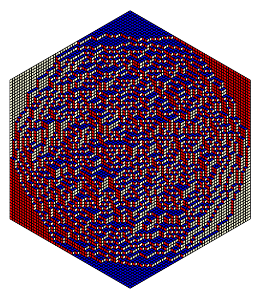
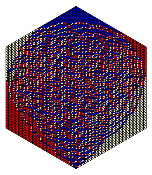
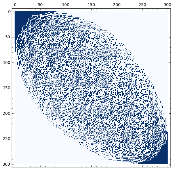
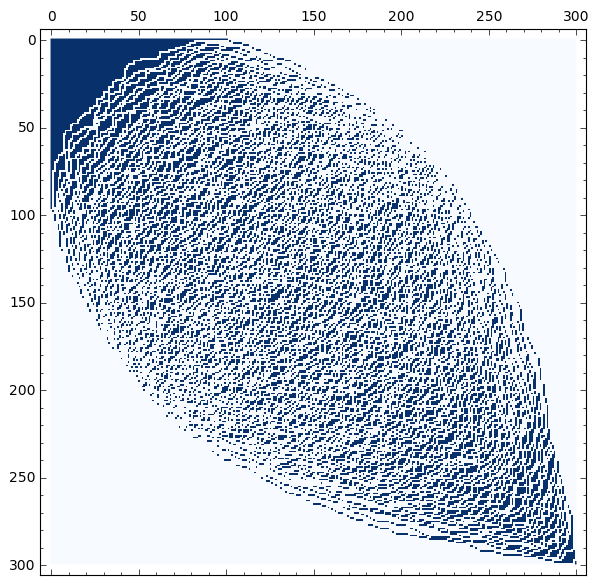
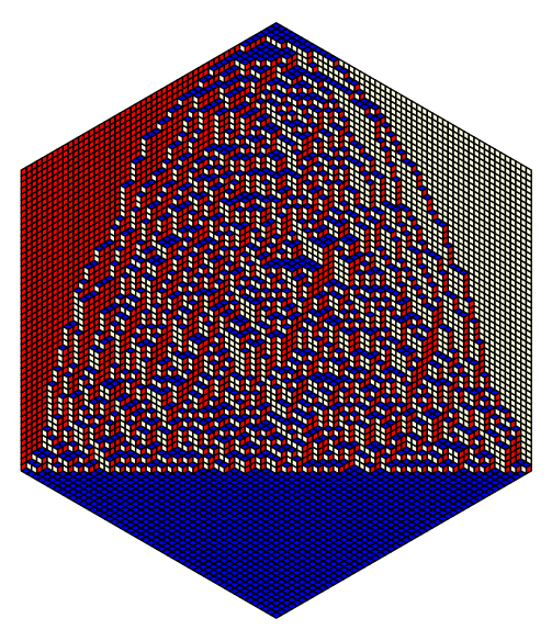
Figure 2. Random tilings of hexagon  H(50,50,50)H505050\operatorname{H}(50,50,50)  with uniform and hook weighted horizontal lozenges.

We illustrate the difference between the uniform and weighted lozenge tilings in Figure 2. Here both tilings of the hexagon H(50,50,50)H505050\operatorname{H}(50,50,50) are obtained by running the Metropolis algorithm for  21092superscript1092\cdot 10^{9}  steps.222In the uniform case, a faster algorithm to generate such random tilings is given in [BG] (see also [Bet]). In the latter case, the weight is defined to be a product over horizontal lozenges of a linear function in the coordinates (see Section 7). Note that the Arctic circle in the uniform case is replaced by a more involved limit shape as in the figure (see also Figure 17). In fact, the results in §§\S8.3 explain why the latter limit shape is tilted upward, even if they are not strong enough to prove its existence (see §§\S9.8).

1.5. Structure of the paper

We begin with a lengthy Section 2 which summarizes the notation and gives a brief review of the earlier work. In the next Section 3, we develop the technology of multivariate formulas including two key identities (Theorems 3.10 and 3.12). We use these identities to prove the product formulas for the number fλ/μsuperscript𝑓𝜆𝜇f^{\lambda/\mu} of SYT of skew shape in Section 4, including generalization of corollaries 1.11.3. In Section 5 we use our technology to obtain product formulas for the principal evaluation of Schubert polynomials. These results are used in Section 6 to obtain asymptotic formulas in a number of special cases. In Section 7, we obtain explicit determinantal formulas for the number of weighted lozenge tilings, which are then interpreted probabilistically and applied in two natural special cases in Section 8. We conclude with final remarks and open problems in Section 9.


2. Notation and Background

2.1. Young diagrams and skew shapes

Let λ=(λ1,,λr),μ=(μ1,,μs)formulae-sequence𝜆subscript𝜆1subscript𝜆𝑟𝜇subscript𝜇1subscript𝜇𝑠\lambda=(\lambda_{1},\ldots,\lambda_{r}),\mu=(\mu_{1},\ldots,\mu_{s}) denote integer partitions of length (λ)=r𝜆𝑟\ell(\lambda)=r and (μ)=s𝜇𝑠\ell(\mu)=s. The size of the partition is denoted by |λ|𝜆|\lambda| and λsuperscript𝜆\lambda^{\prime} denotes the conjugate partition of λ𝜆\lambda. We use [λ]delimited-[]𝜆[\lambda] to denote the Young diagram of the partition λ𝜆\lambda. The hook length hλ(i,j)=λii+λjj+1subscript𝜆𝑖𝑗subscript𝜆𝑖𝑖superscriptsubscript𝜆𝑗𝑗1h_{\lambda}(i,j)=\lambda_{i}-i+\lambda_{j}^{\prime}-j+1 of a square u=(i,j)[λ]𝑢𝑖𝑗delimited-[]𝜆u=(i,j)\in[\lambda] is the number of squares directly to the right or directly below u𝑢u in [λ]delimited-[]𝜆[\lambda] including u𝑢u.

A skew shape is denoted by λ/μ𝜆𝜇\lambda/\mu for partitions μλ𝜇𝜆\mu\subseteq\lambda. The staircase shape is denoted by δn=(n1,n2,,2,1)subscript𝛿𝑛𝑛1𝑛221\delta_{n}=(n-1,n-2,\ldots,2,1). Finally, a skew shape λ/μ𝜆𝜇\lambda/\mu is called slim if λ𝜆\lambda has d𝑑d parts and λdμ1+d1subscript𝜆𝑑subscript𝜇1𝑑1\lambda_{d}\geq\mu_{1}+d-1, see [MPP3, §§\S11].

2.2. Permutations

We write permutations of {1,2,,n}12𝑛\{1,2,\ldots,n\} as w=w1w2wnSn𝑤subscript𝑤1subscript𝑤2subscript𝑤𝑛subscript𝑆𝑛w=w_{1}w_{2}\ldots w_{n}\in S_{n}, where wisubscript𝑤𝑖w_{i} is the image of i𝑖i. Given a positive integer c𝑐c, let 1c×wsuperscript1𝑐𝑤1^{c}\times w denote the direct sum permutation

1c×w:=12c(c+w1)(c+w2)(c+wn).assignsuperscript1𝑐𝑤12𝑐𝑐subscript𝑤1𝑐subscript𝑤2𝑐subscript𝑤𝑛1^{c}\times w\hskip 1.70709pt:=\hskip 1.70709pt1\hskip 0.85355pt2\hskip 0.85355pt\ldots\hskip 0.85355ptc\,(c+w_{1})\hskip 0.85355pt(c+w_{2})\hskip 1.70709pt\ldots\hskip 1.70709pt(c+w_{n})\hskip 1.70709pt.

Similarly, let w1ctensor-product𝑤superscript1𝑐w\otimes 1^{c} denote the Kronecker product permutation of size cn𝑐𝑛\hskip 0.85355ptc\hskip 0.85355ptn\hskip 0.85355pt whose permutation matrix equals the Kronecker product of the permutation matrix Pwsubscript𝑃𝑤P_{w} and the identity matrix Icsubscript𝐼𝑐I_{c}. See Figure 8 for an example.

To each permutation wSn𝑤subscript𝑆𝑛w\in S_{n}, we associate the subset of [n]×[n]delimited-[]𝑛delimited-[]𝑛[n]\times[n] given by

D(w)={(i,wj)i<j,wi>wj}.𝐷𝑤conditional-set𝑖subscript𝑤𝑗formulae-sequence𝑖𝑗subscript𝑤𝑖subscript𝑤𝑗D(w)\hskip 1.70709pt=\hskip 1.70709pt\bigl{\{}(i,w_{j})\hskip 0.85355pt\mid\hskip 0.85355pti<j,\hskip 0.85355ptw_{i}>w_{j}\bigr{\}}\hskip 0.85355pt.

This set is called the (Rothe) diagram of w𝑤w and can be viewed as the complement in [n]×[n]delimited-[]𝑛delimited-[]𝑛[n]\times[n] of the hooks from the cells (i,wi)𝑖subscript𝑤𝑖(i,w_{i}) for i=1,2,,n𝑖12𝑛i=1,2,\ldots,n. The size of this set is the length of w𝑤w and it uniquely determines w𝑤w. Diagrams of permutations play in the theory of Schubert polynomials the role that partitions play in the theory of symmetric functions. The essential set of a permutation w𝑤w is given by

Ess(w)={(i,j)D(w)|(i+1,j),(i,j+1),(i+1,j+1)D(w)}.Ess(w)\hskip 1.70709pt=\hskip 1.70709pt\bigl{\{}(i,j)\in D(w)\,\bigl{|}\,(i+1,j),(i,j+1),(i+1,j+1)\not\in D(w)\bigr{\}}\hskip 0.85355pt.

See Figure 3 for an example of a diagram D(w)𝐷𝑤D(w) and Ess(w)𝐸𝑠𝑠𝑤Ess(w).

Refer to caption
Refer to caption
Refer to caption
Refer to caption
Figure 3. (a) The diagram of the vexillary permutation w=461532𝑤461532w=461532 (with cells in the essential set tiled in red). Up to permuting rows and columns it is the diagram of μ(w)=4321𝜇𝑤4321\mu(w)=4321; the supershape λ(w)=55332𝜆𝑤55332\lambda(w)=55332 defined by the essential set; the skew shape λ(w)/μ(w)𝜆𝑤𝜇𝑤\lambda(w)/\mu(w). (b) Example of correspondence between skew shapes and 321321321-avoiding permutations for w=251634𝑤251634w=251634.

The diagrams of two families of permutations have very appealing properties. These families are also described using the notion of pattern avoidance of permutations [Kit] and play an important role in Schubert calculus. We refer to [Man, §2.1-2] for details and further examples.

A permutation is vexillary if D(w)𝐷𝑤D(w) is, up to permuting rows and columns, the Young diagram of a partition denoted by μ=μ(w)𝜇𝜇𝑤\mu=\mu(w). Equivalently, these are 2143-avoiding permutations, i.e. there is no sequence i<j<k<𝑖𝑗𝑘i<j<k<\ell such that wj<wi<w<wksubscript𝑤𝑗subscript𝑤𝑖subscript𝑤subscript𝑤𝑘w_{j}<w_{i}<w_{\ell}<w_{k}. Given a vexillary permutation let λ=λ(w)𝜆𝜆𝑤\lambda=\lambda(w) be the smallest partition containing the diagram D(w)𝐷𝑤D(w). This partition is also the union over the i×j𝑖𝑗i\times j rectangles with NW–SE corners (1,1)11(1,1), (i,j)𝑖𝑗(i,j) for each (i,j)Ess(w)𝑖𝑗𝐸𝑠𝑠𝑤(i,j)\in Ess(w). We call this partition the supershape of w𝑤w and note that μ(w)λ(w)𝜇𝑤𝜆𝑤\mu(w)\subseteq\lambda(w) (see Figure 3). Examples of vexillary permutations are dominant permutations (132-avoiding) and Grassmannian permutations (permutations with at most one descent).

A permutation is 321-avoiding if there is no sequence i<j<k𝑖𝑗𝑘i<j<k such that wi>wj>wksubscript𝑤𝑖subscript𝑤𝑗subscript𝑤𝑘w_{i}>w_{j}>w_{k}. The diagram D(w)𝐷𝑤D(w) of such a permutation is, up to removing rows and columns of the board not present in the diagram and flipping columns, the Young diagram of a skew shape that we denote skewsh(w)skewsh𝑤\operatorname{skewsh}(w). Conversely, every skew shape λ/μ𝜆𝜇\lambda/\mu can be obtained from the diagram of a 321321321-avoiding permutation [BJS].

Theorem 2.1 (Billey–Jockusch–Stanley [BJS]).

For every skew shape λ/μ𝜆𝜇\lambda/\mu with (n1)𝑛1(n-1) diagonals, there is a 321321321-avoiding permutation wSn𝑤subscript𝑆𝑛w\in S_{n}, such that skewsh(w)=λ/μskewsh𝑤𝜆𝜇\operatorname{skewsh}(w)=\lambda/\mu.

The construction from [BJS] to prove this theorem is as follows: Label the diagonals of λ/μ𝜆𝜇\lambda/\mu from right to left 𝖽𝟣,𝖽𝟤,subscript𝖽1subscript𝖽2\sf{d}_{1},\sf{d}_{2},\ldots and label the cells of λ/μ𝜆𝜇\lambda/\mu by the index of the their diagonal. Let w𝑤w be the permutation whose reduced word is obtained by reading the labeled cells of the skew shape from left to right top to bottom (see Figure 3); we denote this reduced word by rw(λ/μ)rw𝜆𝜇\operatorname{rw}(\lambda/\mu). Note that rw(λ/μ)rw𝜆𝜇\operatorname{rw}(\lambda/\mu) is the lexicographically minimal among the reduced words of w𝑤w.

2.3. Plane partitions

Let PP(a,b,c)PP𝑎𝑏𝑐\operatorname{PP}(a,b,c) and RPP(a,b,c)RPP𝑎𝑏𝑐\operatorname{RPP}(a,b,c) denote the sets of ordinary and reverse plane partitions π𝜋\pi, respectively, that fit into an [a×b×c]delimited-[]𝑎𝑏𝑐\hskip 0.85355pt[a\times b\times c]\hskip 0.85355pt box with nonnegative entries, and let |π|𝜋|\pi| denote the sum of entries of the plane partition. Recall the MacMahon box formula (1.2) for the number of such (reverse) plane partitions, which can also be written as follows:

(2.1) |PP(a,b,c)|=|RPP(a,b,c)|=i=1aj=1bk=1ci+j+k1i+j+k2,PP𝑎𝑏𝑐RPP𝑎𝑏𝑐superscriptsubscriptproduct𝑖1𝑎superscriptsubscriptproduct𝑗1𝑏superscriptsubscriptproduct𝑘1𝑐𝑖𝑗𝑘1𝑖𝑗𝑘2\bigl{|}\operatorname{PP}(a,b,c)\bigr{|}\hskip 1.70709pt=\hskip 1.70709pt\bigl{|}\operatorname{RPP}(a,b,c)\bigr{|}\hskip 1.70709pt=\,\prod_{i=1}^{a}\prod_{j=1}^{b}\prod_{k=1}^{c}\hskip 1.70709pt\frac{i+j+k-1}{i+j+k-2}\,,

and its q𝑞q-analogue:

(2.2) πRPP(a,b,c)q|π|=i=1aj=1bk=1c1qi+j+k11qi+j+k2.subscript𝜋RPP𝑎𝑏𝑐superscript𝑞𝜋superscriptsubscriptproduct𝑖1𝑎superscriptsubscriptproduct𝑗1𝑏superscriptsubscriptproduct𝑘1𝑐1superscript𝑞𝑖𝑗𝑘11superscript𝑞𝑖𝑗𝑘2\sum_{\pi\in\operatorname{RPP}(a,b,c)}q^{|\pi|}\,=\,\prod_{i=1}^{a}\prod_{j=1}^{b}\prod_{k=1}^{c}\,\frac{1-q^{i+j+k-1}}{1-q^{i+j+k-2}}\,.

2.4. Factorial Schur functions

The factorial Schur function (e.g. see [MoS]) is defined as

(2.3) sμ(d)(𝐱𝐚):=det[(xia1)(xiaμj+dj)]i,j=1dΔ(x1,,xd),assignsuperscriptsubscript𝑠𝜇𝑑conditional𝐱𝐚superscriptsubscriptdelimited-[]subscript𝑥𝑖subscript𝑎1subscript𝑥𝑖subscript𝑎subscript𝜇𝑗𝑑𝑗𝑖𝑗1𝑑Δsubscript𝑥1subscript𝑥𝑑s_{\mu}^{(d)}({\bf x}\mid{\bf a}):=\frac{\det\bigl{[}(x_{i}-a_{1})\cdots(x_{i}-a_{\mu_{j}+d-j})\bigr{]}_{i,j=1}^{d}}{\Delta(x_{1},\ldots,x_{d})}\,,

where  𝐱=x1,,xd𝐱subscript𝑥1subscript𝑥𝑑{\bf x}=x_{1},\ldots,x_{d}  are variables,  𝐚=a1,a2,𝐚subscript𝑎1subscript𝑎2{\bf a}=a_{1},a_{2},\ldots  are parameters, and

(2.4) Δ(x1,,xd)=Δ(𝐱):=1i<jd(xixj)Δsubscript𝑥1subscript𝑥𝑑Δ𝐱assignsubscriptproduct1𝑖𝑗𝑑subscript𝑥𝑖subscript𝑥𝑗\Delta(x_{1},\ldots,x_{d})\,=\,\Delta({\bf x}):=\prod_{1\leq i<j\leq d}\hskip 1.70709pt(x_{i}-x_{j})

is the Vandermonde determinant. By convention μj=0subscript𝜇𝑗0\mu_{j}=0 for j>(μ)𝑗𝜇j>\ell(\mu). This function has an explicit expression in terms of semi-standard tableaux of shape μ𝜇\mu :

(2.5) sμ(d)(𝐱|𝐚)=Tuμ(xT(u)aT(u)+c(u)),superscriptsubscript𝑠𝜇𝑑conditional𝐱𝐚subscript𝑇subscriptproduct𝑢𝜇subscript𝑥𝑇𝑢subscript𝑎𝑇𝑢𝑐𝑢s_{\mu}^{(d)}({\bf x}\,|\,{\bf a})\,=\,\sum_{T}\hskip 1.70709pt\prod_{u\in\mu}\hskip 1.70709pt\bigl{(}x_{T(u)}-a_{T(u)+c(u)}\bigr{)}\hskip 0.85355pt,

where the sum is over semistandard Young tableaux T𝑇T of shape μ𝜇\mu with entries in {1,,d}1𝑑\{1,\ldots,d\} and c(u)=ji𝑐𝑢𝑗𝑖c(u)=j-i denotes the content of the cell u=(i,j)𝑢𝑖𝑗u=(i,j). Moreover,  sμ(d)(𝐱|𝐚)superscriptsubscript𝑠𝜇𝑑conditional𝐱𝐚s_{\mu}^{(d)}({\bf x}\,|\,{\bf a})  is symmetric in x1,,xdsubscript𝑥1subscript𝑥𝑑x_{1},\ldots,x_{d}.

2.5. Schubert polynomials

Schubert polynomials were introduced by Lascoux and Schützen-berger [LS1] to study Schubert varieties. We denote by 𝔖w(𝐱;𝐲)subscript𝔖𝑤𝐱𝐲\mathfrak{S}_{w}({\bf x};{\bf y}) the double Schubert polynomial of w𝑤w and by 𝔖w(𝐱)=𝔖w(𝐱;𝟎)subscript𝔖𝑤𝐱subscript𝔖𝑤𝐱0\mathfrak{S}_{w}({\bf x})=\mathfrak{S}_{w}({\bf x};{\bf 0}) the single Schubert polynomial. See [Man, §2.3] and [Mac, §§\SIV,VI] for definitions and properties.

The principal evaluation of a single Schubert polynomials at xi=1subscript𝑥𝑖1x_{i}=1, counting the number of monomials, is given by the following Macdonald identity [Mac, Eq. 6.11] (see also [Man, Thm. 2.5.1] and [BHY] for a bijective proof):

(2.6) Υw:=𝔖w(1,1,,1)=1!(r1,,r)R(w)r1r2r.assignsubscriptΥ𝑤subscript𝔖𝑤1111subscriptsubscript𝑟1subscript𝑟𝑅𝑤subscript𝑟1subscript𝑟2subscript𝑟{\small{\Upsilon}}_{w}\,:=\,\mathfrak{S}_{w}(1,1,\ldots,1)\,=\,\frac{1}{\ell!}\hskip 1.70709pt\sum_{(r_{1},\ldots,r_{\ell})\in R(w)}\hskip 1.70709ptr_{1}r_{2}\cdots r_{\ell}\hskip 1.70709pt.

Here R(w)𝑅𝑤R(w) denotes the set of reduced words of wSn𝑤subscript𝑆𝑛w\in S_{n}\hskip 0.85355pt:  tuples  (r1,r2,,r)subscript𝑟1subscript𝑟2subscript𝑟(r_{1},r_{2},\ldots,r_{\ell})  such that  sr1sr2srsubscript𝑠subscript𝑟1subscript𝑠subscript𝑟2subscript𝑠subscript𝑟s_{r_{1}}s_{r_{2}}\cdots s_{r_{\ell}}  is a reduced decomposition of w𝑤w into simple transpositions si=(i,i+1)subscript𝑠𝑖𝑖𝑖1s_{i}=(i,i+1).

2.6. Excited diagrams

Let λ/μ𝜆𝜇\lambda/\mu be a skew partition and D𝐷D be a subset of the Young diagram of λ𝜆\lambda. A cell u=(i,j)D𝑢𝑖𝑗𝐷u=(i,j)\in D is called active if (i+1,j)𝑖1𝑗(i+1,j), (i,j+1)𝑖𝑗1(i,j+1) and (i+1,j+1)𝑖1𝑗1(i+1,j+1) are all in [λ]Ddelimited-[]𝜆𝐷[\lambda]\setminus D. Let u𝑢u be an active cell of D𝐷D, define αu(D)subscript𝛼𝑢𝐷\alpha_{u}(D) to be the set obtained by replacing (i,j)D𝑖𝑗𝐷(i,j)\in D by (i+1,j+1)𝑖1𝑗1(i+1,j+1). We call this procedure an excited move. An excited diagram of λ/μ𝜆𝜇\lambda/\mu is a subdiagram of λ𝜆\lambda obtained from the Young diagram of μ𝜇\mu after a sequence of excited moves on active cells. Let (λ/μ)𝜆𝜇\mathcal{E}(\lambda/\mu) be the set of excited diagrams of λ/μ𝜆𝜇\lambda/\mu.

Example 2.2.

The skew shape λ/μ=332/21𝜆𝜇33221\lambda/\mu=332/21 has five excited diagrams:

[Uncaptioned image]

.

2.7. Flagged tableaux

Excited diagrams of λ/μ𝜆𝜇\lambda/\mu are equivalent to certain flagged tableaux of shape μ𝜇\mu (see [MPP1, §3] and [Kre, §6]): SSYT of shape μ𝜇\mu with bounds on the entries of each row. The number of excited diagrams is given by a determinant, a polynomial in the parts of λ𝜆\lambda and μ𝜇\mu as follows. Consider the diagonal that passes through cell (i,μi)𝑖subscript𝜇𝑖(i,\mu_{i}), i.e. the last cell of row i𝑖i in μ𝜇\mu. Let this diagonal intersect the boundary of λ𝜆\lambda at a row denoted by 𝖿i(λ/μ)subscriptsuperscript𝖿𝜆𝜇𝑖\mathsf{f}^{(\lambda/\mu)}_{i}. Given an excited diagram D𝐷D in (λ/μ)𝜆𝜇\mathcal{E}(\lambda/\mu), each cell (x,y)𝑥𝑦(x,y) in [μ]delimited-[]𝜇[\mu] corresponds to a cell (i,j)𝑖𝑗(i,j) in D𝐷D, let φ(D):=Tassign𝜑𝐷𝑇\varphi(D):=T be the tableau of shape μ𝜇\mu with Tx,y=isubscript𝑇𝑥𝑦𝑖T_{x,y}=i.

Proposition 2.3 ([MPP1]).

The map φ𝜑\varphi is a bijection between excited diagrams of λ/μ𝜆𝜇\lambda/\mu and SSYT of shape μ𝜇\mu with entries in row i𝑖i at most 𝖿i(λ/μ)subscriptsuperscript𝖿𝜆𝜇𝑖\mathsf{f}^{(\lambda/\mu)}_{i}. Moreover,

|(λ/μ)|=det[(𝖿i(λ/μ)+μii+j1𝖿i(λ/μ)1)]i,j=1(μ).𝜆𝜇superscriptsubscriptdelimited-[]binomialsubscriptsuperscript𝖿𝜆𝜇𝑖subscript𝜇𝑖𝑖𝑗1subscriptsuperscript𝖿𝜆𝜇𝑖1𝑖𝑗1𝜇|\mathcal{E}(\lambda/\mu)|=\det\left[\binom{\mathsf{f}^{(\lambda/\mu)}_{i}+\mu_{i}-i+j-1}{\mathsf{f}^{(\lambda/\mu)}_{i}-1}\right]_{i,j=1}^{\ell(\mu)}.

Note that in the setting of this proposition, bounding all the entries of the SSYT is equivalent to bounding only the entries in the corners of this SSYT.

When the last part of λ𝜆\lambda is long enough relative to the parts of μ𝜇\mu, the number of excited diagrams is given by a product. Recall the notion of slim shapes λ/μ𝜆𝜇\lambda/\mu defined in Section 2.1.

Corollary 2.4.

Let λ/μ𝜆𝜇\lambda/\mu be a slim skew shape,  d=(λ)𝑑𝜆d=\ell(\lambda). Then

|(λ/μ)|=sμ(1d)=(i,j)[μ]d+jiμi+μjij+1.𝜆𝜇subscript𝑠𝜇superscript1𝑑subscriptproduct𝑖𝑗delimited-[]𝜇𝑑𝑗𝑖subscript𝜇𝑖subscriptsuperscript𝜇𝑗𝑖𝑗1|\mathcal{E}(\lambda/\mu)|\,=\,s_{\mu}(1^{d})\,=\,\prod_{(i,j)\in[\mu]}\,\frac{d+j-i}{\mu_{i}+\mu^{\prime}_{j}-i-j+1}\,.
Proof.

In this case, by Proposition 2.3, the excited diagrams of λ/μ𝜆𝜇\lambda/\mu are in bijection with SSYT of shape μ𝜇\mu with entries at most d𝑑d. The number of such SSYT is given by the hook-content formula for sμ(1d)subscript𝑠𝜇superscript1𝑑s_{\mu}(1^{d}), see e.g. [Sta2, Cor. 7.21.4]. ∎

Next we give a family of skew shapes that come up in the paper with product formulas for the number of excited diagrams.

Example 2.5 (thick reverse hook).

For the shape λ/μ=(b+c)a+c/ba𝜆𝜇superscript𝑏𝑐𝑎𝑐superscript𝑏𝑎\lambda/\mu=(b+c)^{a+c}/b^{a}, the excited diagrams correspond to SSYT of shape basuperscript𝑏𝑎b^{a} with entries at most a+c𝑎𝑐a+c. By subtracting i𝑖i from the elements in row i𝑖i these SSYT are equivalent to RPP that fit into an  [a×b×c]delimited-[]𝑎𝑏𝑐[a\times b\times c]\hskip 0.85355pt box. Thus,  |(λ/μ)|=|RPP(a,b,c)|𝜆𝜇RPP𝑎𝑏𝑐|\mathcal{E}(\lambda/\mu)|=|\operatorname{RPP}(a,b,c)|  is given by the MacMahon box formula (1.2).

2.8. Non-intersecting paths

Excited diagrams of λ/μ𝜆𝜇\lambda/\mu are also in bijection with families of non-intersecting grid paths γ1,,γksubscript𝛾1subscript𝛾𝑘\gamma_{1},\ldots,\gamma_{k} with a fixed set of start and end points, which depend only on λ/μ𝜆𝜇\lambda/\mu. A variant of this was proved by Kreiman [Kre, §5-6] (see also [MPP2, §3]).

Formally, given a connected skew shape λ/μ𝜆𝜇\lambda/\mu let γ1subscriptsuperscript𝛾1\gamma^{*}_{1} be the path starting at the northwestern-most box, following the noertwest boundary and ending at the southeastern-most box of the connected component of this skew shape. Clearly, (λ/μ)γ1𝜆𝜇subscriptsuperscript𝛾1(\lambda/\mu)\setminus\gamma^{*}_{1} will be a skew shape. We iterate the construction of the paths on each connected component of this new skew shape ordered bottom to top and obtain a family of non-intersecting paths γ1,,γksubscriptsuperscript𝛾1subscriptsuperscript𝛾𝑘\gamma^{*}_{1},\ldots,\gamma^{*}_{k} in λ𝜆\lambda with support λ/μ𝜆𝜇\lambda/\mu, where each path γisubscriptsuperscript𝛾𝑖\gamma^{*}_{i} starting at a box (ai,bi)subscript𝑎𝑖subscript𝑏𝑖(a_{i},b_{i}) and ending at a box (ci,di)subscript𝑐𝑖subscript𝑑𝑖(c_{i},d_{i}). Let 𝒩𝒫(λ/μ)𝒩𝒫𝜆𝜇\mathcal{NIP}(\lambda/\mu) be the set of k𝑘k-tuples Γ:=(γ1,,γk)assignΓsubscript𝛾1subscript𝛾𝑘\Gamma:=(\gamma_{1},\ldots,\gamma_{k}) of non-intersecting paths contained in [λ]delimited-[]𝜆[\lambda] with γi:(ai,bi)(ci,di):subscript𝛾𝑖subscript𝑎𝑖subscript𝑏𝑖subscript𝑐𝑖subscript𝑑𝑖\gamma_{i}:(a_{i},b_{i})\to(c_{i},d_{i}).

Proposition 2.6 (Kreiman [Kre], see also [MPP2, §3.3]).

Non-intersecting paths in 𝒩𝒫(λ/μ)𝒩𝒫𝜆𝜇\mathcal{NIP}(\lambda/\mu) are uniquely determined by their support, i.e. set of squares. Moreover, the set of such supports is exactly the set of complements [λ]Ddelimited-[]𝜆𝐷[\lambda]\setminus D of excited diagrams D(λ/μ)𝐷𝜆𝜇D\in\mathcal{E}(\lambda/\mu).

Example 2.7.

The complements of excited diagrams in (444/21)44421\mathcal{E}(444/21) correspond to tuples (γ1,γ2)subscript𝛾1subscript𝛾2(\gamma_{1},\gamma_{2}) of nonintersecting paths in [444]delimited-[]444[444] with γ1=(3,1)(1,4)subscript𝛾13114\gamma_{1}=(3,1)\to(1,4) and γ2=(3,3)(2,4)subscript𝛾23324\gamma_{2}=(3,3)\to(2,4):

[Uncaptioned image]
Remark 2.8.

The convention in [Kre, Lemma 5.3] and [MPP2, §3.3] for the paths and starting/ending points is slightly different: the paths begin in the southern box of a column and end at the eastern box of a row instead. However, since the supports of excited diagram of a shape λ/μ𝜆𝜇\lambda/\mu only vary along the diagonals of μ𝜇\mu, then the portions of the paths outside this region will stay the same. Thus, it does not matter how the paths are drawn outside of this region.

[Uncaptioned image]
Remark 2.9.

The excited diagrams of a skew shape have a “path-particle duality” of sorts since they can be viewed as the cells or “particles” of the Young diagram of μ𝜇\mu sliding down the cells of the Young diagram of λ𝜆\lambda and also their complements are in correspondence with certain non-intersecting lattice paths. In the second part of the paper we give two other interpretations of excited diagrams as lozenge tilings and as terms in a known rule for Schubert polynomials of vexillary permutations (see §§\S75).

2.9. The Naruse hook-length formula

Recall the formula of Naruse for fλ/μsuperscript𝑓𝜆𝜇f^{\lambda/\mu} as a sum of products of hook-lengths (see [MPP1, MPP2]).

Theorem 2.10 (NHLF; Naruse [Nar]).

Let λ,μ𝜆𝜇\lambda,\mu be partitions, such that μλ𝜇𝜆\mu\subset\lambda. We have:

(NHLF) fλ/μ=n!D(λ/μ)u[λ]D1h(u),superscript𝑓𝜆𝜇𝑛subscript𝐷𝜆𝜇subscriptproduct𝑢delimited-[]𝜆𝐷1𝑢f^{\lambda/\mu}\,=\,n!\,\sum_{D\in\mathcal{E}(\lambda/\mu)}\,\hskip 1.70709pt\hskip 1.70709pt\prod_{u\in[\lambda]\setminus D}\frac{1}{h(u)}\hskip 1.70709pt\hskip 0.85355pt\hskip 1.70709pt,

where the sum is over all excited diagrams D𝐷D of λ/μ𝜆𝜇\lambda/\mu.

For the q𝑞q-analogues we use a q𝑞q-analogue from [MPP1] for skew semistandard Young tableaux.

Theorem 2.11 ([MPP1]).

We have:333In [MPP1], this is the first q𝑞q-analogue of (NHLF). The second q𝑞q-analogue is in terms of reverse plane partitions.

(q𝑞q-NHLF) sλ/μ(1,q,q2,)=D(λ/μ)(i,j)[λ]Dqλji1qh(i,j).subscript𝑠𝜆𝜇1𝑞superscript𝑞2subscript𝐷𝜆𝜇subscriptproduct𝑖𝑗delimited-[]𝜆𝐷superscript𝑞subscriptsuperscript𝜆𝑗𝑖1superscript𝑞𝑖𝑗s_{\lambda/\mu}(1,q,q^{2},\ldots)\,=\,\sum_{D\in\mathcal{E}(\lambda/\mu)}\hskip 1.70709pt\hskip 1.70709pt\hskip 1.70709pt\prod_{(i,j)\in[\lambda]\setminus D}\frac{q^{\lambda^{\prime}_{j}-i}}{1-q^{h(i,j)}}\hskip 0.85355pt.

These two results were the main object of our study in the two previous papers in the series [MPP1, MPP2]. It is also the key to most results in this paper. However, rather than apply it as “black box” we need to use the technology of multivariate sums in the proof of (NHLF).

2.10. Asymptotics

We use the standard asymptotics notations fgsimilar-to𝑓𝑔f\sim g, f=o(g)𝑓𝑜𝑔f=o(g), f=O(g)𝑓𝑂𝑔f=O(g) and f=Ω(g)𝑓Ω𝑔f=\Omega(g), see e.g. [FS, §§\SA.2]. Recall Stirling’s formula logn!=nlognn+O(logn)𝑛𝑛𝑛𝑛𝑂𝑛\hskip 0.85355pt\log n!=n\log n-n+O(\log n). Here and everywhere below log\hskip 0.85355pt\log\hskip 0.85355pt denotes natural logarithm.

Below is a quick list of asymptotic formulas for other functions in the introduction:

log(2n1)!!=nlogn+(log21)n+O(1),\displaystyle\log\hskip 0.85355pt(2n-1)!!\,=\,n\hskip 0.85355pt\log n\hskip 1.70709pt+\hskip 1.70709pt(\log 2\hskip 0.85355pt-\hskip 0.85355pt1)\hskip 0.85355ptn\hskip 1.70709pt+\hskip 1.70709ptO(1)\hskip 0.85355pt,
logΦ(n)=12n2logn34n2+O(nlogn),Φ𝑛12superscript𝑛2𝑛34superscript𝑛2𝑂𝑛𝑛\displaystyle\log\hskip 0.85355pt\Phi(n)\,=\,\frac{1}{2}\hskip 1.70709ptn^{2}\hskip 0.85355pt\log n\hskip 1.70709pt-\hskip 1.70709pt\frac{3}{4}\hskip 1.70709ptn^{2}\hskip 1.70709pt+\hskip 1.70709ptO(n\hskip 0.85355pt\log n)\hskip 0.85355pt,
logΨ(n)=12n2logn+(log2234)n2+O(nlogn),Ψ𝑛12superscript𝑛2𝑛2234superscript𝑛2𝑂𝑛𝑛\displaystyle\log\hskip 0.85355pt\Psi(n)\,=\,\frac{1}{2}\hskip 0.85355ptn^{2}\hskip 0.85355pt\log n\hskip 1.70709pt+\hskip 1.70709pt\left(\frac{\log 2}{2}\hskip 0.85355pt-\hskip 0.85355pt\frac{3}{4}\right)n^{2}\hskip 1.70709pt+\hskip 1.70709ptO(n\hskip 0.85355pt\log n)\hskip 0.85355pt,
log(n)=14n2logn38n2+O(nlogn),𝑛14superscript𝑛2𝑛38superscript𝑛2𝑂𝑛𝑛\displaystyle\log\hskip 0.85355pt\hskip 0.85355pt\gimel(n)\,=\,\frac{1}{4}\hskip 1.70709ptn^{2}\hskip 0.85355pt\log n\hskip 1.70709pt-\hskip 1.70709pt\frac{3}{8}\hskip 1.70709ptn^{2}\hskip 1.70709pt+\hskip 1.70709ptO(n\hskip 0.85355pt\log n)\hskip 0.85355pt,

see [OEIS, A001147], [OEIS, A008793], [OEIS, A057863], and [OEIS, A113296]. We should also mention that the numbers Φ(n)Φ𝑛\Phi(n) are the integer values of the Barnes G𝐺G-function, whose asymptotics has been extensively studied, see e.g. [AsR].


3. Multivariate path identity

3.1. Multivariate sums of excited diagrams

For the skew shape λ/μd×(nd)𝜆𝜇𝑑𝑛𝑑\lambda/\mu\subseteq d\times(n-d) we define Fλ/μ(𝐱|𝐲)subscript𝐹𝜆𝜇conditional𝐱𝐲F_{\lambda/\mu}({\bf x}\,|\,{\bf y}) and Gλ/μ(𝐱|𝐲)subscript𝐺𝜆𝜇conditional𝐱𝐲G_{\lambda/\mu}({\bf x}\,|\,{\bf y}) to be the multivariate sums of excited diagrams

Gλ/μ(𝐱|𝐲)subscript𝐺𝜆𝜇conditional𝐱𝐲\displaystyle G_{\lambda/\mu}({\bf x}\,|\,{\bf y}) :=D(λ/μ)(i,j)D(xiyj),assignabsentsubscript𝐷𝜆𝜇subscriptproduct𝑖𝑗𝐷subscript𝑥𝑖subscript𝑦𝑗\displaystyle\,:=\,\sum_{D\in\mathcal{E}(\lambda/\mu)}\prod_{(i,j)\in D}(x_{i}-y_{j})\,,
Fλ/μ(𝐱|𝐲)subscript𝐹𝜆𝜇conditional𝐱𝐲\displaystyle F_{\lambda/\mu}({\bf x}\,|\,{\bf y}) :=D(λ/μ)(i,j)[λ]D1xiyj.assignabsentsubscript𝐷𝜆𝜇subscriptproduct𝑖𝑗delimited-[]𝜆𝐷1subscript𝑥𝑖subscript𝑦𝑗\displaystyle\,:=\,\sum_{D\in\mathcal{E}(\lambda/\mu)}\prod_{(i,j)\in[\lambda]\setminus D}\frac{1}{x_{i}-y_{j}}\,.

By Proposition 2.6, the sum  Fλ/μ(𝐱|𝐲)subscript𝐹𝜆𝜇conditional𝐱𝐲F_{\lambda/\mu}({\bf x}\,|\,{\bf y})  can be written as a multivariate sum of non-intersecting paths.

Corollary 3.1.

In the notation above, we have:

Fλ/μ(𝐱|𝐲)=Γ𝒩𝒫(λ/μ)(i,j)Γ1xiyj.subscript𝐹𝜆𝜇conditional𝐱𝐲subscriptΓ𝒩𝒫𝜆𝜇subscriptproduct𝑖𝑗Γ1subscript𝑥𝑖subscript𝑦𝑗F_{\lambda/\mu}({\bf x}\,|\,{\bf y})\,=\hskip 1.70709pt\sum_{\Gamma\in\mathcal{NIP}(\lambda/\mu)}\prod_{(i,j)\in\Gamma}\frac{1}{x_{i}-y_{j}}\,.

Note that by evaluating Fλ/μ(𝐱|𝐲)subscript𝐹𝜆𝜇conditional𝐱𝐲F_{\lambda/\mu}({\bf x}\,|\,{\bf y}) at xi=λii+1subscript𝑥𝑖subscript𝜆𝑖𝑖1x_{i}=\lambda_{i}-i+1 and yj=λj+jsubscript𝑦𝑗subscriptsuperscript𝜆𝑗𝑗y_{j}=-\lambda^{\prime}_{j}+j and multiplying by |λ/μ|!𝜆𝜇|\lambda/\mu|! we obtain the RHS of (NHLF).

(3.1) Fλ/μ(𝐱|𝐲)|xi=λii+1yj=λj+j=fλ/μ|λ/μ|!.evaluated-atsubscript𝐹𝜆𝜇conditional𝐱𝐲subscript𝑥𝑖subscript𝜆𝑖𝑖1subscript𝑦𝑗subscriptsuperscript𝜆𝑗𝑗superscript𝑓𝜆𝜇𝜆𝜇\left.F_{\lambda/\mu}({\bf x}\,|\,{\bf y})\right|_{\begin{subarray}{c}x_{i}=\lambda_{i}-i+1\\ y_{j}=-\lambda^{\prime}_{j}+j\end{subarray}}\,\hskip 1.70709pt=\,\frac{f^{\lambda/\mu}}{|\lambda/\mu|!}\,.

Note that by evaluating (1)|λ/μ|Fλ/μ(𝐱|𝐲)superscript1𝜆𝜇subscript𝐹𝜆𝜇conditional𝐱𝐲(-1)^{|\lambda/\mu|}F_{\lambda/\mu}({\bf x}\,|\,{\bf y}) at xi=qλii+1subscript𝑥𝑖superscript𝑞subscript𝜆𝑖𝑖1x_{i}=q^{\lambda_{i}-i+1} and yj=qλj+jsubscript𝑦𝑗superscript𝑞subscriptsuperscript𝜆𝑗𝑗y_{j}=q^{-\lambda^{\prime}_{j}+j} by (q𝑞q-NHLF) we obtain

(3.2) (1)|λ/μ|Fλ/μ(𝐱|𝐲)|xi=qλii+1yj=qλj+j=qC(λ/μ)sλ/μ(1,q,q2,),evaluated-atsuperscript1𝜆𝜇subscript𝐹𝜆𝜇conditional𝐱𝐲subscript𝑥𝑖superscript𝑞subscript𝜆𝑖𝑖1subscript𝑦𝑗superscript𝑞subscriptsuperscript𝜆𝑗𝑗superscript𝑞𝐶𝜆𝜇subscript𝑠𝜆𝜇1𝑞superscript𝑞2\left.(-1)^{|\lambda/\mu|}F_{\lambda/\mu}({\bf x}\,|\,{\bf y})\right|_{\begin{subarray}{c}x_{i}=q^{\lambda_{i}-i+1}\\ y_{j}=q^{-\lambda^{\prime}_{j}+j}\end{subarray}}\,\hskip 1.70709pt=\,q^{C(\lambda/\mu)}\hskip 0.85355pts_{\lambda/\mu}(1,q,q^{2},\ldots)\hskip 1.70709pt,

where

(3.3) C(λ/μ)=(i,j)λ/μ(ji).𝐶𝜆𝜇subscript𝑖𝑗𝜆𝜇𝑗𝑖C(\lambda/\mu)=\sum_{(i,j)\in\lambda/\mu}(j-i).

The multivariate sum of excited diagrams can be written as an evaluation of a factorial Schur function.

Theorem 3.2 (see [IN]).

For a skew shape λ/μ𝜆𝜇\lambda/\mu inside the rectangle d×(nd)𝑑𝑛𝑑d\times(n-d) we have:

Gλ/μ(𝐱|𝐲)=sμ(d)(yλ1+d,yλ2+d1,,yλd+1|y1,,yn).subscript𝐺𝜆𝜇conditional𝐱𝐲superscriptsubscript𝑠𝜇𝑑subscript𝑦subscript𝜆1𝑑subscript𝑦subscript𝜆2𝑑1conditionalsubscript𝑦subscript𝜆𝑑1subscript𝑦1subscript𝑦𝑛G_{\lambda/\mu}({\bf x}\,|\,{\bf y})\,=\,s_{\mu}^{(d)}(y_{\lambda_{1}+d},y_{\lambda_{2}+d-1},\ldots,y_{\lambda_{d}+1}\,|\,y_{1},\ldots,y_{n}).
Example 3.3.

Continuing with Example 2.5, take the thick reverse hook λ/μ=(b+c)a+c/ba𝜆𝜇superscript𝑏𝑐𝑎𝑐superscript𝑏𝑎\lambda/\mu=(b+c)^{a+c}/b^{a}. When we evaluate  Gλ/μ(𝐱|𝐲)subscript𝐺𝜆𝜇conditional𝐱𝐲G_{\lambda/\mu}({\bf x}\,|\,{\bf y})  at xi=qisubscript𝑥𝑖superscript𝑞𝑖x_{i}=q^{i}, yj=0subscript𝑦𝑗0y_{j}=0, we obtain the q𝑞q-analogue of the MacMahon box formula(2.2) :

(3.4) G(b+c)a+c/ba(q1,q2,| 0,0,)=qb(a+12)i=1aj=1bk=1c1qi+j+k11qi+j+k2.subscript𝐺superscript𝑏𝑐𝑎𝑐superscript𝑏𝑎superscript𝑞1superscript𝑞2conditional 00superscript𝑞𝑏binomial𝑎12superscriptsubscriptproduct𝑖1𝑎superscriptsubscriptproduct𝑗1𝑏superscriptsubscriptproduct𝑘1𝑐1superscript𝑞𝑖𝑗𝑘11superscript𝑞𝑖𝑗𝑘2G_{(b+c)^{a+c}/b^{a}}(q^{1},q^{2},\ldots\,|\,0,0,\ldots)\,=\,q^{b\binom{a+1}{2}}\hskip 1.70709pt\prod_{i=1}^{a}\prod_{j=1}^{b}\prod_{k=1}^{c}\frac{1-q^{i+j+k-1}}{1-q^{i+j+k-2}}\hskip 1.70709pt.

Let 𝐳λsuperscript𝐳delimited-⟨⟩𝜆{\bf z}^{\langle\lambda\rangle} be the tuple of length n𝑛n of x𝑥x’s and y𝑦y’s by reading the horizontal and vertical steps of λ𝜆\lambda from (d,1)𝑑1(d,1) to (1,nd)1𝑛𝑑(1,n-d): i.e. zλi+di+1=xisubscript𝑧subscript𝜆𝑖𝑑𝑖1subscript𝑥𝑖z_{\lambda_{i}+d-i+1}=x_{i} and zd+jλj=yjsubscript𝑧𝑑𝑗subscriptsuperscript𝜆𝑗subscript𝑦𝑗z_{d+j-\lambda^{\prime}_{j}}=y_{j}. For example, for d=4𝑑4d=4, n=9𝑛9n=9 and λ=(5533)𝜆5533\lambda=(5533), we have  𝐳λ=(y1,y2,y3,x4,x3,y4,y5,x2,x1)superscript𝐳delimited-⟨⟩𝜆subscript𝑦1subscript𝑦2subscript𝑦3subscript𝑥4subscript𝑥3subscript𝑦4subscript𝑦5subscript𝑥2subscript𝑥1{\bf z}^{\langle\lambda\rangle}=(y_{1},y_{2},y_{3},x_{4},x_{3},y_{4},y_{5},x_{2},x_{1}):

[Uncaptioned image]

Combining results of Ikeda–Naruse [IN], Knutson–Tao [KT], Lakshmibai–Raghavan–Sankaran [LRS], one obtains the following formula for an evaluation of factorial Schur functions.

Lemma 3.4 (Theorem 2 in [IN]).

For every skew shape  λ/μd×(nd)𝜆𝜇𝑑𝑛𝑑\lambda/\mu\subseteq d\times(n-d), we have:

(3.5) Gλ/μ(𝐱|𝐲)=sμ(d)(𝐱|𝐳λ).subscript𝐺𝜆𝜇conditional𝐱𝐲superscriptsubscript𝑠𝜇𝑑conditional𝐱superscript𝐳delimited-⟨⟩𝜆G_{\lambda/\mu}({\bf x}\,|\,{\bf y})\,=\,s_{\mu}^{(d)}({\bf x}\,|\,{\bf z^{\langle\lambda\rangle}})\hskip 1.70709pt.
Corollary 3.5.

We have:

(3.6) Fλ/μ(𝐱|𝐲)=sμ(d)(𝐱|𝐳λ)sλ(d)(𝐱|𝐳λ).subscript𝐹𝜆𝜇conditional𝐱𝐲superscriptsubscript𝑠𝜇𝑑conditional𝐱superscript𝐳delimited-⟨⟩𝜆superscriptsubscript𝑠𝜆𝑑conditional𝐱superscript𝐳delimited-⟨⟩𝜆F_{\lambda/\mu}({\bf x}\,|\,{\bf y})\,=\,\frac{s_{\mu}^{(d)}({\bf x}\,|\,{\bf z}^{\langle\lambda\rangle})}{s_{\lambda}^{(d)}({\bf x}\,|\,{\bf z}^{\langle\lambda\rangle})}\hskip 1.70709pt.
Proof.

By definition the multivariate polynomial Gλ/λ(𝐱|𝐲)subscript𝐺𝜆𝜆conditional𝐱𝐲G_{\lambda/\lambda}({\bf x}\,|\,{\bf y}) is the product (i,j)[λ](xiyj)subscriptproduct𝑖𝑗delimited-[]𝜆subscript𝑥𝑖subscript𝑦𝑗\prod_{(i,j)\in[\lambda]}(x_{i}-y_{j}) and thus we can write Fλ/μ(𝐱|𝐲)subscript𝐹𝜆𝜇conditional𝐱𝐲F_{\lambda/\mu}({\bf x}\,|\,{\bf y}) as the following quotient

Fλ/μ(𝐱|𝐲)=Gλ/μ(𝐱|𝐲)Gλ/λ(𝐱|𝐲).subscript𝐹𝜆𝜇conditional𝐱𝐲subscript𝐺𝜆𝜇conditional𝐱𝐲subscript𝐺𝜆𝜆conditional𝐱𝐲F_{\lambda/\mu}({\bf x}\,|\,{\bf y})\,=\,\frac{G_{\lambda/\mu}({\bf x}\,|\,{\bf y})}{G_{\lambda/\lambda}({\bf x}\,|\,{\bf y})}.

The result now follows by applying Lemma 3.4 to both the numerator and denominator on the RHS above. ∎

3.2. Symmetries

The factorial Schur function sμ(d)(𝐱|𝐲)subscriptsuperscript𝑠𝑑𝜇conditional𝐱𝐲s^{(d)}_{\mu}({\bf x}\,|\,{\bf y}) is symmetric in x. By Lemma 3.4, the multivariate sum Gλ/μ(𝐱|𝐲)subscript𝐺𝜆𝜇conditional𝐱𝐲G_{\lambda/\mu}({\bf x}\,|\,{\bf y}) is an evaluation of a certain factorial Schur function, which in general is not symmetric in x.

Example 3.6.

The shape λ/μ=332/21𝜆𝜇33221\lambda/\mu=332/21 from Example 2.2 has five excited diagrams. One can check that the multivariate polynomial

G333/21(x1,x2,x3|y1,y2,y3)=(x1y1)(x1y2)(x2y1)+(x1y1)(x1y2)(x3y2)+(x1y1)(x2y3)(x2y1)+(x1y1)(x2y3)(x3y2)+(x2y2)(x2y3)(x3y2),subscript𝐺33321subscript𝑥1subscript𝑥2conditionalsubscript𝑥3subscript𝑦1subscript𝑦2subscript𝑦3subscript𝑥1subscript𝑦1subscript𝑥1subscript𝑦2subscript𝑥2subscript𝑦1subscript𝑥1subscript𝑦1subscript𝑥1subscript𝑦2subscript𝑥3subscript𝑦2subscript𝑥1subscript𝑦1subscript𝑥2subscript𝑦3subscript𝑥2subscript𝑦1subscript𝑥1subscript𝑦1subscript𝑥2subscript𝑦3subscript𝑥3subscript𝑦2subscript𝑥2subscript𝑦2subscript𝑥2subscript𝑦3subscript𝑥3subscript𝑦2G_{333/21}(x_{1},x_{2},x_{3}\,|\,y_{1},y_{2},y_{3})\,=\,(x_{1}-y_{1})(x_{1}-y_{2})(x_{2}-y_{1})\hskip 1.70709pt+\hskip 1.70709pt(x_{1}-y_{1})(x_{1}-y_{2})(x_{3}-y_{2})\\ \qquad\quad+\hskip 1.70709pt(x_{1}-y_{1})(x_{2}-y_{3})(x_{2}-y_{1})\hskip 1.70709pt+\hskip 1.70709pt(x_{1}-y_{1})(x_{2}-y_{3})(x_{3}-y_{2})\hskip 1.70709pt+\hskip 1.70709pt(x_{2}-y_{2})(x_{2}-y_{3})(x_{3}-y_{2})\hskip 0.85355pt,

is not symmetric in x=(x1,x2,x3)xsubscript𝑥1subscript𝑥2subscript𝑥3{\textbf{x}}=(x_{1},x_{2},x_{3}).

Now, below we present two cases when the sum Gλ/μ(𝐱|𝐲)subscript𝐺𝜆𝜇conditional𝐱𝐲G_{\lambda/\mu}({\bf x}\,|\,{\bf y}) is in fact symmetric in x. The first case is when μ𝜇\mu is a rectangle contained in λ𝜆\lambda.

Proposition 3.7.

Let μ=pk𝜇superscript𝑝𝑘\mu=p^{k} be a rectangle, pk𝑝𝑘p\geq k, and let λ𝜆\lambda be arbitrary partition containing μ𝜇\mu. Denote  :=max{i:λiipk}assign:𝑖subscript𝜆𝑖𝑖𝑝𝑘\ell:=\max\{i:\lambda_{i}-i\geq p-k\}. Then:

Gλ/pk(𝐱|𝐲)=spk()(x1,,x|y1,,yp+k).subscript𝐺𝜆superscript𝑝𝑘conditional𝐱𝐲superscriptsubscript𝑠superscript𝑝𝑘subscript𝑥1conditionalsubscript𝑥subscript𝑦1subscript𝑦𝑝𝑘G_{\lambda/p^{k}}({\bf x}\,|\,{\bf y})\,=\,s_{p^{k}}^{(\ell)}(x_{1},\ldots,x_{\ell}\,|\,y_{1},\ldots,y_{p+\ell-k})\hskip 0.85355pt.

In particular, the polynomial  Gλ/pk(𝐱|𝐲)subscript𝐺𝜆superscript𝑝𝑘conditional𝐱𝐲G_{\lambda/p^{k}}({\bf x}\,|\,{\bf y}) is symmetric in (x1,,x)subscript𝑥1subscript𝑥(x_{1},\ldots,x_{\ell}).

Proof.

First, observe that  (λ/pk)=((p+k)/pk)𝜆superscript𝑝𝑘superscript𝑝𝑘superscript𝑝𝑘\mathcal{E}(\lambda/p^{k})=\mathcal{E}((p+\ell-k)^{\ell}/p^{k})  since the movement of the excited boxes is limited by the position of the corner box of pksuperscript𝑝𝑘p^{k}, which moves along the diagonal ji=pk𝑗𝑖𝑝𝑘j-i=p-k up to the boundary of λ𝜆\lambda, at position (,p+k)𝑝𝑘(\ell,p+\ell-k). Thus, the excited diagrams of λ/μ𝜆𝜇\lambda/\mu coincide, as sets of boxes with the excited diagrams of (p+k)/μsuperscript𝑝𝑘𝜇(p+\ell-k)^{\ell}/\mu. Then:

Gλ/pk(𝐱|𝐲)subscript𝐺𝜆superscript𝑝𝑘conditional𝐱𝐲\displaystyle G_{\lambda/p^{k}}({\bf x}\,|\,{\bf y}) =D((p+k)/pk)(i,j)D(xiyj)=G(p+k)/pk(𝐱|𝐲)absentsubscript𝐷superscript𝑝𝑘superscript𝑝𝑘subscriptproduct𝑖𝑗𝐷subscript𝑥𝑖subscript𝑦𝑗subscript𝐺superscript𝑝𝑘superscript𝑝𝑘conditional𝐱𝐲\displaystyle\,=\,\sum_{D\in\mathcal{E}((p+\ell-k)^{\ell}/p^{k})}\prod_{(i,j)\in D}(x_{i}-y_{j})\,=\,G_{(p+\ell-k)^{\ell}/p^{k}}({\bf x}\,|\,{\bf y})
=spk()(x1,,x|𝐳(p+k)).absentsuperscriptsubscript𝑠superscript𝑝𝑘subscript𝑥1conditionalsubscript𝑥superscript𝐳delimited-⟨⟩superscript𝑝𝑘\displaystyle\,=\,s_{p^{k}}^{(\ell)}\bigl{(}x_{1},\ldots,x_{\ell}\,|\,{\bf z}^{\langle(p+\ell-k)^{\ell}\rangle}\bigr{)}\hskip 1.70709pt.

Note that 𝐳(p+k)=(y1,,yp+k,x,,x1)superscript𝐳delimited-⟨⟩superscript𝑝𝑘subscript𝑦1subscript𝑦𝑝𝑘subscript𝑥subscript𝑥1{\bf z}^{\langle(p+\ell-k)^{\ell}\rangle}=(y_{1},\ldots,y_{p+\ell-k},x_{\ell},\ldots,x_{1}). Let us now invoke the original combinatorial formula for the factorial Schur functions, equation (2.5), with aj=yjsubscript𝑎𝑗subscript𝑦𝑗a_{j}=y_{j} for jp+k𝑗𝑝𝑘j\leq p+\ell-k and ap+k+j=x+1jsubscript𝑎𝑝𝑘𝑗subscript𝑥1𝑗a_{p+\ell-k+j}=x_{\ell+1-j} otherwise. Note also that when T𝑇T is an SSYT of shape pksuperscript𝑝𝑘p^{k} and entries at most \ell, by the strictness of columns we have T(i,j)(ki)𝑇𝑖𝑗𝑘𝑖T(i,j)\leq\ell-(k-i) for all entries in row i𝑖i. We conclude:

T(u)+c(u)(ki)+ji=k+jk+p.𝑇𝑢𝑐𝑢𝑘𝑖𝑗𝑖𝑘𝑗𝑘𝑝T(u)+c(u)\leq\ell-(k-i)+j-i=\ell-k+j\leq\ell-k+p\hskip 1.70709pt.

Therefore,  aT(u)+c(u)=yT(u)+c(u)subscript𝑎𝑇𝑢𝑐𝑢subscript𝑦𝑇𝑢𝑐𝑢a_{T(u)+c(u)}=y_{T(u)+c(u)}, where only the first p+k𝑝𝑘p+\ell-k parameters aisubscript𝑎𝑖a_{i} are involved in the formula. Then:

sμ()(x,,x1|a1,,ap+k,ap+k+1,)superscriptsubscript𝑠𝜇subscript𝑥conditionalsubscript𝑥1subscript𝑎1subscript𝑎𝑝𝑘subscript𝑎𝑝𝑘1\displaystyle s_{\mu}^{(\ell)}(x_{\ell},\ldots,x_{1}\,|\,a_{1},\ldots,a_{p+\ell-k},a_{p+\ell-k+1},\ldots) =sμ()(x,,x1|a1,,ap+k)absentsuperscriptsubscript𝑠𝜇subscript𝑥conditionalsubscript𝑥1subscript𝑎1subscript𝑎𝑝𝑘\displaystyle\,=\,s_{\mu}^{(\ell)}(x_{\ell},\ldots,x_{1}\,|\,a_{1},\ldots,a_{p+\ell-k})
=sμ()(x1,,x|y1,,yp+k),absentsuperscriptsubscript𝑠𝜇subscript𝑥1conditionalsubscript𝑥subscript𝑦1subscript𝑦𝑝𝑘\displaystyle\,=\,s_{\mu}^{(\ell)}(x_{1},\ldots,x_{\ell}\,|\,y_{1},\ldots,y_{p+\ell-k}),

since now the parameters of the factorial Schur are independent of the variables 𝐱𝐱{\bf x} and the function is also symmetric in 𝐱𝐱{\bf x}. ∎

The second symmetry involves slim skew shapes (see Section 2.1). An example includes a skew shape λ/μ𝜆𝜇\lambda/\mu, where λ𝜆\lambda is the rectangle (nd)dsuperscript𝑛𝑑𝑑(n-d)^{d} and μ1n2d+1subscript𝜇1𝑛2𝑑1\mu_{1}\leq n-2d+1.

Proposition 3.8.

Let λ/μ𝜆𝜇\lambda/\mu be a slim skew shape inside the rectangle d×(nd)𝑑𝑛𝑑d\times(n-d). Then:

Gλ/μ(𝐱|𝐲)=sμ(d)(x1,,xd|y1,,yλd).subscript𝐺𝜆𝜇conditional𝐱𝐲superscriptsubscript𝑠𝜇𝑑subscript𝑥1conditionalsubscript𝑥𝑑subscript𝑦1subscript𝑦subscript𝜆𝑑G_{\lambda/\mu}({\bf x}\,|\,{\bf y})\,=\,s_{\mu}^{(d)}(x_{1},\ldots,x_{d}\,|\,y_{1},\ldots,y_{\lambda_{d}})\hskip 0.85355pt.

In particular, the polynomial  Gλ/μ(𝐱|𝐲)subscript𝐺𝜆𝜇conditional𝐱𝐲G_{\lambda/\mu}({\bf x}\,|\,{\bf y})  is symmetric in (x1,,xd)subscript𝑥1subscript𝑥𝑑(x_{1},\ldots,x_{d}).

Proof.

Note that 𝐳λ=(y1,,yλd,xd,)superscript𝐳delimited-⟨⟩𝜆subscript𝑦1subscript𝑦subscript𝜆𝑑subscript𝑥𝑑\hskip 0.85355pt{\bf z}^{\langle\lambda\rangle}=(y_{1},\ldots,y_{\lambda_{d}},x_{d},\ldots). Note also that for all j=1,,d𝑗1𝑑j=1,\ldots,d,

μj+djλdd+1+djλdλj,subscript𝜇𝑗𝑑𝑗subscript𝜆𝑑𝑑1𝑑𝑗subscript𝜆𝑑subscript𝜆𝑗\mu_{j}+d-j\leq\lambda_{d}-d+1+d-j\leq\lambda_{d}\leq\lambda_{j},

and so z1,,zμj+dj=y1,,yμj+djformulae-sequencesubscript𝑧1subscript𝑧subscript𝜇𝑗𝑑𝑗subscript𝑦1subscript𝑦subscript𝜇𝑗𝑑𝑗z_{1},\ldots,z_{\mu_{j}+d-j}=y_{1},\ldots,y_{\mu_{j}+d-j}. Next, we evaluate the factorial Schur function on the RHS of (3.5) via its determinantal formula (2.3). We obtain:

Gλ/μ(𝐱|𝐲)subscript𝐺𝜆𝜇conditional𝐱𝐲\displaystyle G_{\lambda/\mu}({\bf x}\,|\,{\bf y}) =sμ(d)(x1,,xd|z1,,zn)=det[(xd+1iz1)(xd+1izμj+dj)]i,j=1dΔ(x1,,xd)absentsuperscriptsubscript𝑠𝜇𝑑subscript𝑥1conditionalsubscript𝑥𝑑subscript𝑧1subscript𝑧𝑛superscriptsubscriptdelimited-[]subscript𝑥𝑑1𝑖subscript𝑧1subscript𝑥𝑑1𝑖subscript𝑧subscript𝜇𝑗𝑑𝑗𝑖𝑗1𝑑Δsubscript𝑥1subscript𝑥𝑑\displaystyle\hskip 1.70709pt=\hskip 1.70709pts_{\mu}^{(d)}(x_{1},\ldots,x_{d}\,|\,z_{1},\ldots,z_{n})\hskip 1.70709pt=\hskip 1.70709pt\frac{\det[(x_{d+1-i}-z_{1})\cdots(x_{d+1-i}-z_{\mu_{j}+d-j})]_{i,j=1}^{d}}{\Delta(x_{1},\ldots,x_{d})}
=det[(xiy1)(xiyμj+dj)]i,j=1dΔ(x1,,xd)=sμ(d)(x1,,xd|y1,,yλd),absentsuperscriptsubscriptdelimited-[]subscript𝑥𝑖subscript𝑦1subscript𝑥𝑖subscript𝑦subscript𝜇𝑗𝑑𝑗𝑖𝑗1𝑑Δsubscript𝑥1subscript𝑥𝑑superscriptsubscript𝑠𝜇𝑑subscript𝑥1conditionalsubscript𝑥𝑑subscript𝑦1subscript𝑦subscript𝜆𝑑\displaystyle=\hskip 1.70709pt\frac{\det[(x_{i}-y_{1})\cdots(x_{i}-y_{\mu_{j}+d-j})]_{i,j=1}^{d}}{\Delta(x_{1},\ldots,x_{d})}\hskip 1.70709pt=\hskip 1.70709pts_{\mu}^{(d)}(x_{1},\ldots,x_{d}\,|\,y_{1},\ldots,y_{\lambda_{d}})\hskip 0.85355pt,

where the last equality is by the same determinantal formula. ∎

Example 3.9.

For λ/μ=444/21𝜆𝜇44421\lambda/\mu=444/21, the multivariate sum G444/21(x1,x2,x3|y1,y2,y3,y4)subscript𝐺44421subscript𝑥1subscript𝑥2conditionalsubscript𝑥3subscript𝑦1subscript𝑦2subscript𝑦3subscript𝑦4G_{444/21}(x_{1},x_{2},x_{3}\,|\,y_{1},y_{2},y_{3},y_{4}) of the eight excited diagrams in (444/21)44421\mathcal{E}(444/21) is symmetric in x1,x2,x3subscript𝑥1subscript𝑥2subscript𝑥3x_{1},x_{2},x_{3}.

3.3. Multivariate path identities

We give two identities for the multivariate sums over non-intersecting paths as applications of each of Propositions 3.7 and 3.8.

Refer to caption
Figure 4. Left: paths and flipped paths in Theorem 3.10. Right: paths and flipped paths in Theorem 3.12.
Theorem 3.10.

We have the following identity for multivariate rational functions:

(3.7) Γ=(γ1,,γc)γp:(a+p,1)(p,b+c)(i,j)Γ1xiyj=Θ=(θ1,,θc)θp:(p,1)(a+p,b+c)(i,j)Θ1xiyj,subscriptΓsubscript𝛾1subscript𝛾𝑐:subscript𝛾𝑝𝑎𝑝1𝑝𝑏𝑐subscriptproduct𝑖𝑗Γ1subscript𝑥𝑖subscript𝑦𝑗subscriptΘsubscript𝜃1subscript𝜃𝑐:subscript𝜃𝑝𝑝1𝑎𝑝𝑏𝑐subscriptproduct𝑖𝑗Θ1subscript𝑥𝑖subscript𝑦𝑗\sum_{\begin{subarray}{c}\Gamma=(\gamma_{1},\ldots,\gamma_{c})\\ \gamma_{p}:(a+p,1)\to(p,b+c)\end{subarray}}\prod_{(i,j)\in\Gamma}\frac{1}{x_{i}-y_{j}}\ \,=\sum_{\begin{subarray}{c}\Theta=(\theta_{1},\ldots,\theta_{c})\\ \theta_{p}:(p,1)\to(a+p,b+c)\end{subarray}}\prod_{(i,j)\in\Theta}\frac{1}{x_{i}-y_{j}}\,,

where the sums are over non-intersecting lattice paths as above. Note that the LHS is equal to  F(b+c)a+c/ba(𝐱|𝐲)subscript𝐹superscript𝑏𝑐𝑎𝑐superscript𝑏𝑎conditional𝐱𝐲F_{(b+c)^{a+c}/b^{a}}({\bf x}\,|\,{\bf y})  defined above.

In the next section we use this identity to obtain product formulas for fλ/μsuperscript𝑓𝜆𝜇f^{\lambda/\mu} for certain families of shapes λ/μ𝜆𝜇\lambda/\mu. In the case c=1𝑐1c=1, we evaluate (3.8) at xi=isubscript𝑥𝑖𝑖x_{i}=i and yj=j+1subscript𝑦𝑗𝑗1y_{j}=-j+1 obtain the following corollary.

Corollary 3.11 ([MPP1]).

We have:

(3.8) γ:(a,1)(1,b)(i,j)γ1i+j1=γ:(1,1)(a,b)(i,j)γ1i+j1.subscript:𝛾𝑎11𝑏subscriptproduct𝑖𝑗𝛾1𝑖𝑗1subscript:𝛾11𝑎𝑏subscriptproduct𝑖𝑗𝛾1𝑖𝑗1\sum_{\gamma:(a,1)\to(1,b)}\prod_{(i,j)\in\gamma}\frac{1}{i+j-1}\ =\sum_{\gamma:(1,1)\to(a,b)}\prod_{(i,j)\in\gamma}\frac{1}{i+j-1}\,.

Equation (3.8) is a special case of (NHLF) for the skew shape (b+1)a+1/basuperscript𝑏1𝑎1superscript𝑏𝑎(b+1)^{a+1}/b^{a} [MPP1, §3.1]. This equation is also a special case of Racah formulas in [BGR, §10] (see in § 9.6).

Proof of Theorem 3.10.

By Proposition 3.8 for the shape (b+c)a+c/basuperscript𝑏𝑐𝑎𝑐superscript𝑏𝑎(b+c)^{a+c}/b^{a}, we have:

G(b+c)a+c/ba(𝐱|𝐲)=sba(x1,,xa+c|y1,,yb+c).subscript𝐺superscript𝑏𝑐𝑎𝑐superscript𝑏𝑎conditional𝐱𝐲subscript𝑠superscript𝑏𝑎subscript𝑥1conditionalsubscript𝑥𝑎𝑐subscript𝑦1subscript𝑦𝑏𝑐G_{(b+c)^{a+c}/b^{a}}({\bf x}\,|\,{\bf y})\,=\,s_{b^{a}}(x_{1},\ldots,x_{a+c}\,\,|\,\,y_{1},\ldots,y_{b+c})\hskip 1.70709pt.

Divide the LHS by (i,j)(b+c)a+c(xiyj)subscriptproduct𝑖𝑗superscript𝑏𝑐𝑎𝑐subscript𝑥𝑖subscript𝑦𝑗\prod_{(i,j)\in(b+c)^{a+c}}(x_{i}-y_{j}) to obtain F(b+c)a+c/ba(𝐱|𝐲)subscript𝐹superscript𝑏𝑐𝑎𝑐superscript𝑏𝑎conditional𝐱𝐲F_{(b+c)^{a+c}/b^{a}}({\bf x}\,|\,{\bf y}), the multivariate sum over excited diagrams. By Corollary 3.1, this is also a multivariate sum over tuples of non-intersecting paths in 𝒩𝒫((b+c)a+c/ba)𝒩𝒫superscript𝑏𝑐𝑎𝑐superscript𝑏𝑎\mathcal{NIP}((b+c)^{a+c}/b^{a}) :

(3.9) Γ=(γ1,,γc)γp:(a+p,1)(p,b+c)(i,j)Γ1xiyj=sba(x1,,xa+c|y1,,yb+c)(i,j)(b+c)a+c1xiyj.subscriptΓsubscript𝛾1subscript𝛾𝑐:subscript𝛾𝑝𝑎𝑝1𝑝𝑏𝑐subscriptproduct𝑖𝑗Γ1subscript𝑥𝑖subscript𝑦𝑗subscript𝑠superscript𝑏𝑎subscript𝑥1conditionalsubscript𝑥𝑎𝑐subscript𝑦1subscript𝑦𝑏𝑐subscriptproduct𝑖𝑗superscript𝑏𝑐𝑎𝑐1subscript𝑥𝑖subscript𝑦𝑗\sum_{\begin{subarray}{c}\Gamma=(\gamma_{1},\ldots,\gamma_{c})\\ \gamma_{p}:(a+p,1)\to(p,b+c)\end{subarray}}\prod_{(i,j)\in\Gamma}\frac{1}{x_{i}-y_{j}}\,=\,s_{b^{a}}(x_{1},\ldots,x_{a+c}\,\,|\,\,y_{1},\ldots,y_{b+c})\prod_{(i,j)\in(b+c)^{a+c}}\frac{1}{x_{i}-y_{j}}\,.

Finally, the symmetry in x1,,xa+csubscript𝑥1subscript𝑥𝑎𝑐x_{1},\ldots,x_{a+c} of the RHS above implies that we can flip these variables and consequently the paths γpsubscriptsuperscript𝛾𝑝\gamma^{\prime}_{p} to paths θp:(p,1)(a+p,b+c):subscript𝜃𝑝𝑝1𝑎𝑝𝑏𝑐\theta_{p}:(p,1)\to(a+p,b+c) (see Figure 4), and obtain the needed expression. ∎

For a partition μ𝜇\mu inside the rectangle d×(nd)𝑑𝑛𝑑d\times(n-d) of length \ell, let μ^^𝜇\widehat{\mu} denote the tuple (0d,μ,μ1,,μ1)superscript0𝑑subscript𝜇subscript𝜇1subscript𝜇1(0^{d-\ell},\mu_{\ell},\mu_{\ell-1},\ldots,\mu_{1}).

Theorem 3.12.

Let λ/μd×(nd)𝜆𝜇𝑑𝑛𝑑\lambda/\mu\subset d\times(n-d) be a slim skew shape. Then:

(3.10) Γ𝒩𝒫(λ/μ)(i,j)Γ1xiyj=Γ𝒩𝒫(λ/μ^)(i,j)Γ1xiyj.subscriptΓ𝒩𝒫𝜆𝜇subscriptproduct𝑖𝑗Γ1subscript𝑥𝑖subscript𝑦𝑗subscriptΓ𝒩𝒫𝜆^𝜇subscriptproduct𝑖𝑗Γ1subscript𝑥𝑖subscript𝑦𝑗\sum_{\Gamma\in\mathcal{NIP}(\lambda/\mu)}\prod_{(i,j)\in\Gamma}\frac{1}{x_{i}-y_{j}}=\sum_{\Gamma\in\mathcal{NIP}(\lambda/\widehat{\mu})}\prod_{(i,j)\in\Gamma}\frac{1}{x_{i}-y_{j}}\,.
Proof.

By Proposition 3.7 for the shape λ/μ𝜆𝜇\lambda/\mu we have that

G(nd)d/μ(𝐱|𝐲)=sμ(d)(x1,,xd|y1,,yλd).subscript𝐺superscript𝑛𝑑𝑑𝜇conditional𝐱𝐲superscriptsubscript𝑠𝜇𝑑subscript𝑥1conditionalsubscript𝑥𝑑subscript𝑦1subscript𝑦subscript𝜆𝑑G_{(n-d)^{d}/\mu}({\bf x}\,|\,{\bf y})=s_{\mu}^{(d)}(x_{1},\ldots,x_{d}\,|\,y_{1},\ldots,y_{\lambda_{d}}).

The rest of the proof follows mutatis mutandis that of Theorem 3.10 for the shape λ/μ𝜆𝜇\lambda/\mu instead of the shape (b+c)a+c/basuperscript𝑏𝑐𝑎𝑐superscript𝑏𝑎(b+c)^{a+c}/b^{a}. See Figure 4. ∎

Remark 3.13.

In [MPP5] we use this second symmetry identity to give new lower bounds on fλ/μsuperscript𝑓𝜆𝜇f^{\lambda/\mu} for several other families of slim shapes λ/μ𝜆𝜇\lambda/\mu.

3.4. Variant of excited diagrams for rectangles and slim shapes

Recall that for μd×(nd)𝜇𝑑𝑛𝑑\mu\subseteq d\times(n-d) of length \ell, we denote by μ^^𝜇\widehat{\mu} the tuple  (𝟎d,μ,μ1,,μ1)superscript0𝑑subscript𝜇subscript𝜇1subscript𝜇1({\bf 0}^{d-\ell},\mu_{\ell},\mu_{\ell-1},\ldots,\mu_{1}). We interpret the complements of the supports of the paths in 𝒩𝒫((b+c)a+c/0cba)𝒩𝒫superscript𝑏𝑐𝑎𝑐superscript0𝑐superscript𝑏𝑎\mathcal{NIP}\bigl{(}(b+c)^{a+c}/0^{c}b^{a}\bigr{)} and in 𝒩𝒫(λ/μ^)𝒩𝒫𝜆^𝜇\mathcal{NIP}(\lambda/\widehat{\mu}), as variants of excited diagrams.

A NE-excited diagram of shape λ/μ𝜆𝜇\lambda/\mu is a subdiagram of λ𝜆\lambda obtained from the Young diagram of ba^=(0cba)^superscript𝑏𝑎superscript0𝑐superscript𝑏𝑎\widehat{b^{a}}=(0^{c}b^{a}) (and μ^^𝜇\widehat{\mu}) after a sequence of moves from (i,j)𝑖𝑗(i,j) to (i1,j+1)𝑖1𝑗1(i-1,j+1) provided (i,j)𝑖𝑗(i,j) is in the subdiagram D𝐷D and all of (i1,j),(i1,j+1),(i,j+1)𝑖1𝑗𝑖1𝑗1𝑖𝑗1(i-1,j),(i-1,j+1),(i,j+1) are in [λ]Ddelimited-[]𝜆𝐷[\lambda]\setminus D. We denote the set of such diagrams by (λ/μ)superscript𝜆𝜇\mathcal{E}^{\nearrow}(\lambda/\mu). Analogous to Proposition 2.6, the complements of these diagrams correspond to tuples of paths in 𝒩𝒫((b+c)a+c/0cba)𝒩𝒫superscript𝑏𝑐𝑎𝑐superscript0𝑐superscript𝑏𝑎\mathcal{NIP}\bigl{(}(b+c)^{a+c}/0^{c}b^{a}\bigr{)} (in 𝒩𝒫(λ/μ^)𝒩𝒫𝜆^𝜇\mathcal{NIP}(\lambda/\widehat{\mu})). Flipping horizontally the  [d×λd]delimited-[]𝑑subscript𝜆𝑑[d\times\lambda_{d}]  rectangle gives a bijection between excited diagrams and NE-excited diagrams of λ/μ𝜆𝜇\lambda/\mu. Thus

|(λ/μ)|=|(λ/μ)|.superscript𝜆𝜇𝜆𝜇\bigl{|}\mathcal{E}^{\nearrow}(\lambda/\mu)\bigr{|}\hskip 1.70709pt=\hskip 1.70709pt\bigl{|}\mathcal{E}(\lambda/\mu)\bigr{|}\hskip 0.85355pt.

Moreover, equation (3.10) states that such a flip also preserves the multivariate series Fλ/μ(𝐱|𝐲)subscript𝐹𝜆𝜇conditional𝐱𝐲F_{\lambda/\mu}({\bf x}\,|\,{\bf y}) and polynomial Gλ/μ(𝐱|𝐲)subscript𝐺𝜆𝜇conditional𝐱𝐲G_{\lambda/\mu}({\bf x}\,|\,{\bf y}).

Corollary 3.14.

We have:

(3.11) F(b+c)a+c/ba(𝐱|𝐲)=D((b+c)a+c/0cba)(i,j)[λ]D1xiyj,subscript𝐹superscript𝑏𝑐𝑎𝑐superscript𝑏𝑎conditional𝐱𝐲subscript𝐷superscriptsuperscript𝑏𝑐𝑎𝑐superscript0𝑐superscript𝑏𝑎subscriptproduct𝑖𝑗delimited-[]𝜆𝐷1subscript𝑥𝑖subscript𝑦𝑗F_{(b+c)^{a+c}/b^{a}}({\bf x}\,|\,{\bf y})\,=\,\sum_{D\in\mathcal{E}^{\nearrow}\bigl{(}(b+c)^{a+c}/0^{c}b^{a}\bigr{)}}\prod_{(i,j)\in[\lambda]\setminus D}\frac{1}{x_{i}-y_{j}}\,,

and

(3.12) G(b+c)a+c/ba(𝐱|𝐲)=D((b+c)a+c/0cba)(i,j)D(xiyj).subscript𝐺superscript𝑏𝑐𝑎𝑐superscript𝑏𝑎conditional𝐱𝐲subscript𝐷superscriptsuperscript𝑏𝑐𝑎𝑐superscript0𝑐superscript𝑏𝑎subscriptproduct𝑖𝑗𝐷subscript𝑥𝑖subscript𝑦𝑗G_{(b+c)^{a+c}/b^{a}}({\bf x}\,|\,{\bf y})\,=\,\sum_{D\in\mathcal{E}^{\nearrow}\bigl{(}(b+c)^{a+c}/0^{c}b^{a}\bigr{)}}\prod_{(i,j)\in D}(x_{i}-y_{j})\,.
Proof.

This follows from the discussion above, Corollary 3.1 and Theorem 3.10. ∎

Corollary 3.15.

For a slim skew shape λ/μ𝜆𝜇\lambda/\mu, we have:

(3.13) Fλ/μ(𝐱|𝐲)=D(λ/μ)(i,j)[λ]D1xiyj.subscript𝐹𝜆𝜇conditional𝐱𝐲subscript𝐷superscript𝜆𝜇subscriptproduct𝑖𝑗delimited-[]𝜆𝐷1subscript𝑥𝑖subscript𝑦𝑗F_{\lambda/\mu}({\bf x}\,|\,{\bf y})\,=\,\sum_{D\in\mathcal{E}^{\nearrow}(\lambda/\mu)}\prod_{(i,j)\in[\lambda]\setminus D}\frac{1}{x_{i}-y_{j}}\,.
Proof.

This follows from the discussion above, Corollary 3.1 and Theorem 3.12. ∎


4. Skew shapes with product formulas

In this section we use Theorem 3.10 to obtain product formulas for a family of skew shapes.

4.1. Six-parameter family of skew shapes

For all  a,b,c,d,e,m𝑎𝑏𝑐𝑑𝑒𝑚a,b,c,d,e,m\in\mathbb{N}, let  Λ(a,b,c,d,e,m)Λ𝑎𝑏𝑐𝑑𝑒𝑚\Lambda(a,b,c,d,e,m)  denote the skew shape λ/ba𝜆superscript𝑏𝑎\lambda/b^{a}, where λ𝜆\lambda is given by

(4.1) λ:=(b+c)a+c+(νθ),assign𝜆superscript𝑏𝑐𝑎𝑐𝜈superscript𝜃\lambda\hskip 1.70709pt:=\hskip 1.70709pt(b+c)^{a+c}\hskip 1.70709pt+\hskip 1.70709pt\bigl{(}\nu\cup\theta^{\prime}\bigr{)}\hskip 1.70709pt,

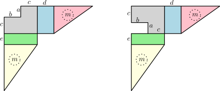
and where ν=(d+(a+c1)m,d+(a+c2)m,,d)𝜈𝑑𝑎𝑐1𝑚𝑑𝑎𝑐2𝑚𝑑\hskip 0.85355pt\nu=(d+(a+c-1)m,d+(a+c-2)m,\ldots,d),  θ=(e+(b+c1)m,e+(b+c2)m,,e)𝜃𝑒𝑏𝑐1𝑚𝑒𝑏𝑐2𝑚𝑒\theta=(e+(b+c-1)m,e+(b+c-2)m,\ldots,e); see Figure 5.  This shape satisfies two key properties:

(P1) λa+c+1subscript𝜆𝑎𝑐1\displaystyle\lambda_{a+c+1} b+c,absent𝑏𝑐\displaystyle\leq b+c\hskip 0.85355pt,
(P2) λi+λjsubscript𝜆𝑖subscriptsuperscript𝜆𝑗\displaystyle\lambda_{i}+\lambda^{\prime}_{j} =λr+λs, if i+j=r+s and (i,j),(r,s)(b+c)a+c.formulae-sequenceabsentsubscript𝜆𝑟subscriptsuperscript𝜆𝑠formulae-sequence if 𝑖𝑗𝑟𝑠 and 𝑖𝑗𝑟𝑠superscript𝑏𝑐𝑎𝑐\displaystyle=\lambda_{r}+\lambda^{\prime}_{s},\quad\text{ if }i+j=r+s\text{ and }(i,j),(r,s)\in(b+c)^{a+c}\hskip 0.85355pt.

The second property implies that λiλi+1=λjλj+1subscript𝜆𝑖subscript𝜆𝑖1subscriptsuperscript𝜆𝑗subscriptsuperscript𝜆𝑗1\lambda_{i}-\lambda_{i+1}=\lambda^{\prime}_{j}-\lambda^{\prime}_{j+1} for all ia+c1𝑖𝑎𝑐1i\leq a+c-1 and jb+c1𝑗𝑏𝑐1j\leq b+c-1, and therefore λiλi+1subscript𝜆𝑖subscript𝜆𝑖1\lambda_{i}-\lambda_{i+1} is independent of i𝑖i, i.e. the parts of λ𝜆\lambda are given by an arithmetic progression. Also, the antidiagonals in (b+c)a+csuperscript𝑏𝑐𝑎𝑐(b+c)^{a+c} inside λ𝜆\lambda have the same hook-lengths.

Here are two extreme special cases:

Λ(a,b,c,0,0,1)=δa+b+2c/ba,Λ(a,b,c,d,e,0)=(b+c+d)a+c(b+c)e/ba.formulae-sequenceΛ𝑎𝑏𝑐001subscript𝛿𝑎𝑏2𝑐superscript𝑏𝑎Λ𝑎𝑏𝑐𝑑𝑒0superscript𝑏𝑐𝑑𝑎𝑐superscript𝑏𝑐𝑒superscript𝑏𝑎\Lambda(a,b,c,0,0,1)\hskip 1.70709pt=\hskip 1.70709pt\delta_{a+b+2c}/b^{a}\,,\qquad\Lambda(a,b,c,d,e,0)\hskip 1.70709pt=\hskip 1.70709pt(b+c+d)^{a+c}(b+c)^{e}/b^{a}\hskip 1.70709pt.

Note that these shapes are depicted in Figure 1(ii) and Figure 1(i), respectively.
Refer to caption
Figure 5. Left: Skew shape Λ(a,b,c,d,e,m)Λ𝑎𝑏𝑐𝑑𝑒𝑚\Lambda(a,b,c,d,e,m). Right: the cells whose hook-lengths appear in the product formula of Theorem 4.1.

Next, we give a product formula for fπsuperscript𝑓𝜋f^{\pi} where π=Λ(a,b,c,d,e,m)𝜋Λ𝑎𝑏𝑐𝑑𝑒𝑚\pi=\Lambda(a,b,c,d,e,m) in terms of falling superfactorials

Ψ(m)(n):=i=1n1j=1i(jm+j1)m,where(k)m=k(k1)(km+1).formulae-sequenceassignsuperscriptΨ𝑚𝑛superscriptsubscriptproduct𝑖1𝑛1superscriptsubscriptproduct𝑗1𝑖subscript𝑗𝑚𝑗1𝑚wheresubscript𝑘𝑚𝑘𝑘1𝑘𝑚1\Psi^{(m)}(n)\,:=\,\prod_{i=1}^{n-1}\hskip 1.70709pt\prod_{j=1}^{i}\,(jm+j-1)_{m}\,,\quad\text{where}\quad(k)_{m}\hskip 1.70709pt=\hskip 1.70709ptk(k-1)\cdots(k-m+1).

Note that Ψ(0)(n)=1superscriptΨ0𝑛1\Psi^{(0)}(n)=1 and Ψ(1)(n)=Ψ(n)superscriptΨ1𝑛Ψ𝑛\Psi^{(1)}(n)=\Psi(n).

Theorem 4.1.

Let  π=Λ(a,b,c,d,e,m)𝜋Λ𝑎𝑏𝑐𝑑𝑒𝑚\pi=\Lambda(a,b,c,d,e,m)  be as above. Then  fπsuperscript𝑓𝜋f^{\pi}  is given by the following product:

(4.2) fπsuperscript𝑓𝜋\displaystyle f^{\pi} =n!i=1aj=1bk=1ci+j+k1i+j+k2(i,j)λ/(0cba)1hλ(i,j),absent𝑛superscriptsubscriptproduct𝑖1𝑎superscriptsubscriptproduct𝑗1𝑏superscriptsubscriptproduct𝑘1𝑐𝑖𝑗𝑘1𝑖𝑗𝑘2subscriptproduct𝑖𝑗𝜆superscript0𝑐superscript𝑏𝑎1subscript𝜆𝑖𝑗\displaystyle\,=\,\hskip 1.70709ptn!\cdot\prod_{i=1}^{a}\prod_{j=1}^{b}\prod_{k=1}^{c}\hskip 1.70709pt\frac{i+j+k-1}{i+j+k-2}\cdot\,\prod_{(i,j)\in\lambda/(0^{c}b^{a})}\,\frac{1}{h_{\lambda}(i,j)}\,,
(4.3) =n!Φ(a+b+c)Φ(a)Φ(b)Φ(c)Φ(a+b)Φ(b+c)Φ(a+c)Ψ(m)(a+c)Ψ(m)(b+c)×\displaystyle\,=\,\hskip 1.70709ptn!\hskip 1.70709pt\cdot\hskip 1.70709pt\frac{\Phi(a+b+c)\hskip 1.70709pt\Phi(a)\hskip 1.70709pt\Phi(b)\hskip 1.70709pt\Phi(c)}{\Phi(a+b)\hskip 1.70709pt\Phi(b+c)\hskip 1.70709pt\Phi(a+c)\hskip 1.70709pt\Psi^{(m)}(a+c)\hskip 1.70709pt\Psi^{(m)}(b+c)}\,\hskip 1.70709pt\times
×i=0a+c1(i(m+1))!(d+i(m+1))!i=0b+c1(i(m+1))!(e+i(m+1))!i=0b1j=0a1(1+d+e+(c+i+j)(m+1))i=0b+c1j=0a+c1(1+d+e+(i+j)(m+1)).\displaystyle\times\prod_{i=0}^{a+c-1}\frac{(i(m+1))!}{(d+i(m+1))!}\,\hskip 1.70709pt\prod_{i=0}^{b+c-1}\frac{(i(m+1))!}{(e+i(m+1))!}\,\,\frac{\prod_{i=0}^{b-1}\prod_{j=0}^{a-1}(1+d+e+(c+i+j)(m+1))}{\prod_{i=0}^{b+c-1}\prod_{j=0}^{a+c-1}(1+d+e+(i+j)(m+1))}\,.
Proof of Corollaries 1.1, 1.2 and 1.3.

Use (4.3) for the shapes Λ(a,b,c,e,d,0)Λ𝑎𝑏𝑐𝑒𝑑0\Lambda(a,b,c,e,d,0), Λ(a,b,c,0,0,1)Λ𝑎𝑏𝑐001\Lambda(a,b,c,0,0,1), and Λ(a,b,c,d,e,1)Λ𝑎𝑏𝑐𝑑𝑒1\Lambda(a,b,c,d,e,1), respectively. ∎

We also give a product formula for the generating function of SSYT of these shapes.

Theorem 4.2.

Let π=Λ(a,b,c,d,e,m)𝜋Λ𝑎𝑏𝑐𝑑𝑒𝑚\pi=\Lambda(a,b,c,d,e,m) be as above. Then:

(4.4) sπ(1,q,q2,)=qNi=1aj=1bk=1c1q(m+1)(i+j+k1)1q(m+1)(i+j+k2)(i,j)λ/(0cba)11qhλ(i,j),subscript𝑠𝜋1𝑞superscript𝑞2superscript𝑞𝑁superscriptsubscriptproduct𝑖1𝑎superscriptsubscriptproduct𝑗1𝑏superscriptsubscriptproduct𝑘1𝑐1superscript𝑞𝑚1𝑖𝑗𝑘11superscript𝑞𝑚1𝑖𝑗𝑘2subscriptproduct𝑖𝑗𝜆superscript0𝑐superscript𝑏𝑎11superscript𝑞subscript𝜆𝑖𝑗s_{\pi}(1,q,q^{2},\ldots)\,=\,q^{N}\hskip 1.70709pt\prod_{i=1}^{a}\prod_{j=1}^{b}\prod_{k=1}^{c}\hskip 1.70709pt\frac{1-q^{(m+1)(i+j+k-1)}}{1-q^{(m+1)(i+j+k-2)}}\,\prod_{(i,j)\in\lambda/(0^{c}b^{a})}\hskip 1.70709pt\frac{1}{1-q^{h_{\lambda}(i,j)}}\,,

where N=(i,j)λ/ba(λji)𝑁subscript𝑖𝑗𝜆superscript𝑏𝑎subscriptsuperscript𝜆𝑗𝑖\hskip 0.85355ptN\hskip 0.85355pt=\hskip 0.85355pt\sum_{(i,j)\in\lambda/b^{a}}(\lambda^{\prime}_{j}-i).

As in the proof above, we obtain explicit formulas for the skew shapes Λ(a,b,c,d,e,0)Λ𝑎𝑏𝑐𝑑𝑒0\Lambda(a,b,c,d,e,0), Λ(a,b,c,0,0,1)Λ𝑎𝑏𝑐001\Lambda(a,b,c,0,0,1), and Λ(a,b,c,d,e,1)Λ𝑎𝑏𝑐𝑑𝑒1\Lambda(a,b,c,d,e,1). By comparing (4.3) and (4.4), up to the power of q𝑞q, these cases are obtained by “q𝑞q-ifying” their counterpart formulas for fλ/μsuperscript𝑓𝜆𝜇f^{\lambda/\mu}. The formulas are written in terms of:

q𝑞q-factorials [m]!delimited-[]𝑚[m]! :=assign:= (1q)(1q2)(1qm)1𝑞1superscript𝑞21superscript𝑞𝑚(1-q)(1-q^{2})\cdots(1-q^{m})
q𝑞q-double factorials [2n1]!!double-factorialdelimited-[]2𝑛1[2n-1]!! :=assign:= (1q)(1q3)(1q2n1)1𝑞1superscript𝑞31superscript𝑞2𝑛1(1-q)(1-q^{3})\cdots(1-q^{2n-1})
q𝑞q-superfactorials Φq(n)subscriptΦ𝑞𝑛\Phi_{q}(n) :=assign:= [1]![2]![n1]!delimited-[]1delimited-[]2delimited-[]𝑛1[1]!\cdot[2]!\hskip 1.70709pt\cdots\hskip 1.70709pt[n-1]!
q𝑞q-super doublefactorials Ψq(n)subscriptΨ𝑞𝑛\Psi_{q}(n) :=assign:= [1]!![3]!![2n3]!!double-factorialdelimited-[]1double-factorialdelimited-[]3double-factorialdelimited-[]2𝑛3[1]!!\hskip 1.70709pt\cdot\hskip 1.70709pt[3]!!\cdots[2n-3]!!
q𝑞q-double superfactorial q(n)subscript𝑞𝑛\gimel_{q}(n) :=assign:= [n2]![n4]!delimited-[]𝑛2delimited-[]𝑛4[n-2]!\hskip 1.70709pt[n-4]!\hskip 1.70709pt\cdots\hskip 1.70709pt
q𝑞q-shifted super doublefactorial Ψq(n;k)subscriptΨ𝑞𝑛𝑘\Psi_{q}(n;k) :=assign:= [k+1]!![k+3]!![k+2n3]!!double-factorialdelimited-[]𝑘1double-factorialdelimited-[]𝑘3double-factorialdelimited-[]𝑘2𝑛3[k+1]!!\hskip 1.70709pt[k+3]!!\hskip 1.70709pt\cdots\hskip 1.70709pt[k+2n-3]!!

Note that in the classical notation [m]!=1qi1qdelimited-[]𝑚product1superscript𝑞𝑖1𝑞[m]!=\prod\frac{1-q^{i}}{1-q} (e.g. from [Sta2]), however here the factors of (1q)1𝑞(1-q) are omitted, otherwise the formulas below would have an additional factor of (1q)|π|superscript1𝑞𝜋(1-q)^{|\pi|}.

Corollary 4.3.

For the skew shape  π=Λ(a,b,c,d,e,0)𝜋Λ𝑎𝑏𝑐𝑑𝑒0\pi=\Lambda(a,b,c,d,e,0), we have:

sπ(1,q,)=qNΦq(a)Φq(b)Φq(c)Φq(d)Φq(e)Φq(a+b+c)Φq(c+d+e)Φq(a+b+c+d+e)Φq(a+b)Φq(d+e)Φq(a+c+d)Φq(b+c+e)Φq(a+b+2c+d+e),subscript𝑠𝜋1𝑞superscript𝑞𝑁subscriptΦ𝑞𝑎subscriptΦ𝑞𝑏subscriptΦ𝑞𝑐subscriptΦ𝑞𝑑subscriptΦ𝑞𝑒subscriptΦ𝑞𝑎𝑏𝑐subscriptΦ𝑞𝑐𝑑𝑒subscriptΦ𝑞𝑎𝑏𝑐𝑑𝑒subscriptΦ𝑞𝑎𝑏subscriptΦ𝑞𝑑𝑒subscriptΦ𝑞𝑎𝑐𝑑subscriptΦ𝑞𝑏𝑐𝑒subscriptΦ𝑞𝑎𝑏2𝑐𝑑𝑒s_{\pi}(1,q,\ldots)\,=\,\frac{q^{N}\hskip 0.85355pt\Phi_{q}(a)\hskip 0.85355pt\Phi_{q}(b)\hskip 0.85355pt\Phi_{q}(c)\hskip 0.85355pt\Phi_{q}(d)\hskip 0.85355pt\Phi_{q}(e)\hskip 0.85355pt\Phi_{q}(a+b+c)\hskip 0.85355pt\Phi_{q}(c+d+e)\hskip 0.85355pt\Phi_{q}(a+b+c+d+e)}{\Phi_{q}(a+b)\hskip 0.85355pt\Phi_{q}(d+e)\hskip 0.85355pt\Phi_{q}(a+c+d)\hskip 0.85355pt\Phi_{q}(b+c+e)\hskip 0.85355pt\Phi_{q}(a+b+2c+d+e)}\,,

where N=b(c+e2)+c(a+c+e2)+d(a+c2)𝑁𝑏binomial𝑐𝑒2𝑐binomial𝑎𝑐𝑒2𝑑binomial𝑎𝑐2\hskip 0.85355ptN=b\binom{c+e}{2}+c\binom{a+c+e}{2}+d\binom{a+c}{2}.

Note that this is a q𝑞q-analogue of Corollary 4.3 by Kim and Oh (see also §§\S9.3).

Corollary 4.4 (Krattenthaler–Schlosser [KS], see §9.4).

For the skew shape  π=Λ(a,b,c,0,0,1)𝜋Λ𝑎𝑏𝑐001\pi=\Lambda(a,b,c,0,0,1), we have:

sπ(1,q,)=qNΦq(a)Φq(b)Φq(c)Φq(a+b+c)Ψq(c)Ψq(a+b+c)Φq(a+b)Φq(b+c)Φq(a+c)Ψq(a+c)Ψq(b+c)Ψq(a+b+2c),subscript𝑠𝜋1𝑞superscript𝑞𝑁subscriptΦ𝑞𝑎subscriptΦ𝑞𝑏subscriptΦ𝑞𝑐subscriptΦ𝑞𝑎𝑏𝑐subscriptΨ𝑞𝑐subscriptΨ𝑞𝑎𝑏𝑐subscriptΦ𝑞𝑎𝑏subscriptΦ𝑞𝑏𝑐subscriptΦ𝑞𝑎𝑐subscriptΨ𝑞𝑎𝑐subscriptΨ𝑞𝑏𝑐subscriptΨ𝑞𝑎𝑏2𝑐s_{\pi}(1,q,\ldots)\,=\,q^{N}\,\frac{\Phi_{q}(a)\hskip 1.70709pt\Phi_{q}(b)\hskip 1.70709pt\Phi_{q}(c)\hskip 1.70709pt\Phi_{q}(a+b+c)\hskip 0.85355pt\cdot\hskip 0.85355pt\Psi_{q}(c)\Psi_{q}(a+b+c)}{\Phi_{q}(a+b)\hskip 1.70709pt\Phi_{q}(b+c)\hskip 1.70709pt\Phi_{q}(a+c)\hskip 0.85355pt\cdot\hskip 0.85355pt\Psi_{q}(a+c)\Psi_{q}(b+c)\Psi_{q}(a+b+2c)}\,,

where N=(a+b+2c3)+b(a+12)+a(b+12)ab(a+b+2c)𝑁binomial𝑎𝑏2𝑐3𝑏binomial𝑎12𝑎binomial𝑏12𝑎𝑏𝑎𝑏2𝑐N=\binom{a+b+2c}{3}+b\binom{a+1}{2}+a\binom{b+1}{2}-ab(a+b+2c).

Corollary 4.5.

For the skew shape  π=Λ(a,b,c,d,e,1)𝜋Λ𝑎𝑏𝑐𝑑𝑒1\pi=\Lambda(a,b,c,d,e,1), we have:

sπ(1,q,)=qNΦq(a)Φq(b)Φq(c)Φq(a+b+c)Φq(a+b)Φq(b+c)Φq(a+c)××Ψq(c;d+e)Ψq(a+b+c;d+e)q(2a+2c)q(2b+2c)Ψq(a+b+2c;d+e)Ψq(a+c)Ψq(b+c)q(d)q(e)q(2a+2c+d)q(2b+2c+e).subscript𝑠𝜋1𝑞superscript𝑞𝑁subscriptΦ𝑞𝑎subscriptΦ𝑞𝑏subscriptΦ𝑞𝑐subscriptΦ𝑞𝑎𝑏𝑐subscriptΦ𝑞𝑎𝑏subscriptΦ𝑞𝑏𝑐subscriptΦ𝑞𝑎𝑐subscriptΨ𝑞𝑐𝑑𝑒subscriptΨ𝑞𝑎𝑏𝑐𝑑𝑒subscript𝑞2𝑎2𝑐subscript𝑞2𝑏2𝑐subscriptΨ𝑞𝑎𝑏2𝑐𝑑𝑒subscriptΨ𝑞𝑎𝑐subscriptΨ𝑞𝑏𝑐subscript𝑞𝑑subscript𝑞𝑒subscript𝑞2𝑎2𝑐𝑑subscript𝑞2𝑏2𝑐𝑒s_{\pi}(1,q,\ldots)\,=\,q^{N}\,\frac{\Phi_{q}(a)\hskip 1.70709pt\Phi_{q}(b)\hskip 1.70709pt\Phi_{q}(c)\hskip 1.70709pt\Phi_{q}(a+b+c)}{\Phi_{q}(a+b)\hskip 1.70709pt\Phi_{q}(b+c)\hskip 1.70709pt\Phi_{q}(a+c)}\,\times\\ \qquad\times\,\frac{\Psi_{q}(c;d+e)\hskip 1.70709pt\Psi_{q}(a+b+c;d+e)\hskip 0.85355pt\cdot\hskip 0.85355pt\,\gimel_{q}(2a+2c)\hskip 1.70709pt\gimel_{q}(2b+2c)}{\Psi_{q}(a+b+2c;d+e)\hskip 1.70709pt\Psi_{q}(a+c)\hskip 1.70709pt\Psi_{q}(b+c)\hskip 0.85355pt\cdot\hskip 0.85355pt\gimel_{q}(d)\hskip 0.85355pt\gimel_{q}(e)\hskip 0.85355pt\gimel_{q}(2a+2c+d)\hskip 1.70709pt\gimel_{q}(2b+2c+e)}\,.

where N=(a+b+2c+e3)+d(a+c2)+(a+c3)(a+c+e3)+b(a+12)+a(b+12)ab(a+b+2c+e)𝑁binomial𝑎𝑏2𝑐𝑒3𝑑binomial𝑎𝑐2binomial𝑎𝑐3binomial𝑎𝑐𝑒3𝑏binomial𝑎12𝑎binomial𝑏12𝑎𝑏𝑎𝑏2𝑐𝑒N=\binom{a+b+2c+e}{3}+d\binom{a+c}{2}+\binom{a+c}{3}-\binom{a+c+e}{3}+b\binom{a+1}{2}+a\binom{b+1}{2}-ab(a+b+2c+e).

Proof of Corollaries 4.3, 4.4, and 4.5.

We “q𝑞q-ify” the formula in corollaries  1.1, 1.2, and 1.3 respectively and calculate the corresponding power of q𝑞q in (4.4) to obtain the stated formula. ∎

The rest of the section is devoted to the proof of Theorem 4.1 and Theorem 4.2.

4.2. Proof of the product formulas for skew SYT

Proof of Theorem 4.1.

The starting point is showing that the skew shape λ/ba=Λ(a,b,c,d,e,m)𝜆superscript𝑏𝑎Λ𝑎𝑏𝑐𝑑𝑒𝑚\lambda/b^{a}=\Lambda(a,b,c,d,e,m) and the thick reverse hook  (b+c)a+c/ba=Λ(a,b,c,0,0,0)superscript𝑏𝑐𝑎𝑐superscript𝑏𝑎Λ𝑎𝑏𝑐000(b+c)^{a+c}/b^{a}=\Lambda(a,b,c,0,0,0)  have the same excited diagrams. To simplify the notation, let R=(b+c)a+c𝑅superscript𝑏𝑐𝑎𝑐R=(b+c)^{a+c} be the rectangle  [(a+c)×(b+c)]delimited-[]𝑎𝑐𝑏𝑐\bigl{[}(a+c)\times(b+c)\bigr{]}.

Lemma 4.6.

The skew shapes Λ(a,b,c,d,e,m)Λ𝑎𝑏𝑐𝑑𝑒𝑚\Lambda(a,b,c,d,e,m) and Λ(a,b,c,0,0,0)=R/baΛ𝑎𝑏𝑐000𝑅superscript𝑏𝑎\Lambda(a,b,c,0,0,0)=R/b^{a} have the same excited diagrams.

Proof.

This can be seen directly from the description of excited diagrams: by property (P1) from Section 4.1, the cell (b,a)𝑏𝑎(b,a) of [μ]delimited-[]𝜇[\mu] cannot go past the cell (b+c,a+c)𝑏𝑐𝑎𝑐(b+c,a+c) so the rest of [μ]delimited-[]𝜇[\mu] is confined in the rectangle (b+c)a+csuperscript𝑏𝑐𝑎𝑐(b+c)^{a+c}. Alternatively by Proposition 2.3, the excited diagrams of both shapes correspond to SSYT of shape basuperscript𝑏𝑎b^{a} with entries at most b+c𝑏𝑐b+c. Then the map φ1superscript𝜑1\varphi^{-1} applied to such tableaux yields the same excited diagrams. ∎

By (NHLF) and Lemma 4.6 we have:

(4.5) fλ/ban!=[u[λ]R1hλ(i,j)]D(R/ba)(i,j)RD1hλ(i,j).superscript𝑓𝜆superscript𝑏𝑎𝑛delimited-[]subscriptproduct𝑢delimited-[]𝜆𝑅1subscript𝜆𝑖𝑗subscript𝐷𝑅superscript𝑏𝑎subscriptproduct𝑖𝑗𝑅𝐷1subscript𝜆𝑖𝑗\frac{f^{\lambda/b^{a}}}{n!}\,=\,\left[\prod_{u\in[\lambda]\setminus R}\,\frac{1}{h_{\lambda}(i,j)}\right]\,\sum_{D\in\mathcal{E}(R/b^{a})}\prod_{(i,j)\in R\setminus D}\frac{1}{h_{\lambda}(i,j)}\,.

The sum over excited diagrams of R/ba𝑅superscript𝑏𝑎R/b^{a} with hook-lengths in λ𝜆\lambda on the RHS above evaluates to a product.

Lemma 4.7.

For λ𝜆\lambda and R𝑅R as above we have:

(4.6) D(R/ba)(i,j)RD1hλ(i,j)=Φ(a+b+c)Φ(a)Φ(b)Φ(c)Φ(a+b)Φ(b+c)Φ(a+c)(i,j)R/0cba1hλ(i,j).subscript𝐷𝑅superscript𝑏𝑎subscriptproduct𝑖𝑗𝑅𝐷1subscript𝜆𝑖𝑗Φ𝑎𝑏𝑐Φ𝑎Φ𝑏Φ𝑐Φ𝑎𝑏Φ𝑏𝑐Φ𝑎𝑐subscriptproduct𝑖𝑗𝑅superscript0𝑐superscript𝑏𝑎1subscript𝜆𝑖𝑗\sum_{D\in\mathcal{E}(R/b^{a})}\prod_{(i,j)\in R\setminus D}\frac{1}{h_{\lambda}(i,j)}\,=\,\frac{\Phi(a+b+c)\hskip 1.70709pt\Phi(a)\hskip 1.70709pt\Phi(b)\hskip 1.70709pt\Phi(c)}{\Phi(a+b)\hskip 1.70709pt\Phi(b+c)\hskip 1.70709pt\Phi(a+c)}\,\prod_{(i,j)\in R/0^{c}b^{a}}\,\frac{1}{h_{\lambda}(i,j)}\,.
Proof.

We write the sum of excited diagrams as an evaluation of  F(b+c)a+c/ba(𝐱|𝐲)subscript𝐹superscript𝑏𝑐𝑎𝑐superscript𝑏𝑎conditional𝐱𝐲F_{(b+c)^{a+c}/b^{a}}({\bf x}\,|\,{\bf y}).

(4.7) D(R/ba)(i,j)RD1hλ(i,j)=F(b+c)a+c/ba(𝐱|𝐲)|xi=λii+1yj=jλjsubscript𝐷𝑅superscript𝑏𝑎subscriptproduct𝑖𝑗𝑅𝐷1subscript𝜆𝑖𝑗evaluated-atsubscript𝐹superscript𝑏𝑐𝑎𝑐superscript𝑏𝑎conditional𝐱𝐲subscript𝑥𝑖subscript𝜆𝑖𝑖1subscript𝑦𝑗𝑗subscriptsuperscript𝜆𝑗\sum_{D\in\mathcal{E}(R/b^{a})}\prod_{(i,j)\in R\setminus D}\frac{1}{h_{\lambda}(i,j)}\,=\,\left.F_{(b+c)^{a+c}/b^{a}}({\bf x}\,|\,{\bf y})\right|_{\begin{subarray}{c}x_{i}=\lambda_{i}-i+1\\ y_{j}=j-\lambda^{\prime}_{j}\end{subarray}}

where m=(b+c)(a+c)ba𝑚𝑏𝑐𝑎𝑐𝑏𝑎m=(b+c)(a+c)-ba. Using Theorem 3.10 to obtain the symmetry of the series F(b+c)a+c/ba(𝐱|𝐲)subscript𝐹superscript𝑏𝑐𝑎𝑐superscript𝑏𝑎conditional𝐱𝐲F_{(b+c)^{a+c}/b^{a}}({\bf x}\,|\,{\bf y}) in x :

(4.8) F(b+c)a+c/ba(𝐱|𝐲)|xi=λii+1yj=jλj=Θ(i,j)Θ1hλ(i,j),evaluated-atsubscript𝐹superscript𝑏𝑐𝑎𝑐superscript𝑏𝑎conditional𝐱𝐲subscript𝑥𝑖subscript𝜆𝑖𝑖1subscript𝑦𝑗𝑗subscriptsuperscript𝜆𝑗subscriptΘsubscriptproduct𝑖𝑗Θ1subscript𝜆𝑖𝑗\left.F_{(b+c)^{a+c}/b^{a}}({\bf x}\,|\,{\bf y})\right|_{\begin{subarray}{c}x_{i}=\lambda_{i}-i+1\\ y_{j}=j-\lambda^{\prime}_{j}\end{subarray}}\,=\,\sum_{\Theta}\prod_{(i,j)\in\Theta}\frac{1}{h_{\lambda}(i,j)}\,,

where the sum is over tuples Θ:=(θ1,,θc)assignΘsubscript𝜃1subscript𝜃𝑐\hskip 0.85355pt\Theta:=(\theta_{1},\ldots,\theta_{c})  of nonintersecting paths inside (b+c)a+csuperscript𝑏𝑐𝑎𝑐(b+c)^{a+c} with endpoints  θp:(p,1)(a+p,b+c):subscript𝜃𝑝𝑝1𝑎𝑝𝑏𝑐\theta_{p}:(p,1)\to(a+p,b+c). Note that each tuple ΘΘ\Theta has the same number of cells in each diagonal i+j=k𝑖𝑗𝑘i+j=k. Also, by property (P2) of λ𝜆\lambda, the sum  λi+λjsubscript𝜆𝑖subscriptsuperscript𝜆𝑗\lambda_{i}+\lambda^{\prime}_{j}  is constant when  i+j𝑖𝑗i+j  is constant. Thus each tuple ΘΘ\Theta will have the same contribution to the sum on the RHS of (4.8), namely

(i,j)Θ1hλ(i,j)=(i,j)R/0cba1hλ(i,j).subscriptproduct𝑖𝑗Θ1subscript𝜆𝑖𝑗subscriptproduct𝑖𝑗𝑅superscript0𝑐superscript𝑏𝑎1subscript𝜆𝑖𝑗\prod_{(i,j)\in\Theta}\hskip 1.70709pt\frac{1}{h_{\lambda}(i,j)}\,=\,\prod_{(i,j)\in R/0^{c}b^{a}}\frac{1}{h_{\lambda}(i,j)}\,.

Lastly, the number of tuples ΘΘ\Theta in (4.8) equals the number of excited diagrams (b+c)a+c/basuperscript𝑏𝑐𝑎𝑐superscript𝑏𝑎(b+c)^{a+c}/b^{a}, given by (1.2), see Example 2.5. ∎

By Lemma 4.7, (4.5) becomes the following product formula for fλ/ba/n!superscript𝑓𝜆superscript𝑏𝑎𝑛f^{\lambda/b^{a}}/n! equivalent to (4.2) :

(4.9) fλ/ban!=Φ(a+b+c)Φ(a)Φ(b)Φ(c)Φ(a+b)Φ(b+c)Φ(a+c)(i,j)λ/0cba1hλ(i,j).superscript𝑓𝜆superscript𝑏𝑎𝑛Φ𝑎𝑏𝑐Φ𝑎Φ𝑏Φ𝑐Φ𝑎𝑏Φ𝑏𝑐Φ𝑎𝑐subscriptproduct𝑖𝑗𝜆superscript0𝑐superscript𝑏𝑎1subscript𝜆𝑖𝑗\frac{f^{\lambda/b^{a}}}{n!}\,=\,\frac{\Phi(a+b+c)\hskip 1.70709pt\Phi(a)\hskip 1.70709pt\Phi(b)\hskip 1.70709pt\Phi(c)}{\Phi(a+b)\hskip 1.70709pt\Phi(b+c)\hskip 1.70709pt\Phi(a+c)}\,\prod_{(i,j)\in\lambda/0^{c}b^{a}}\,\frac{1}{h_{\lambda}(i,j)}\,.

See Figure 5 for an illustration of the cells of [λ]delimited-[]𝜆[\lambda] whose hook-lengths appear above. Finally, we carefully rewrite this product in terms of Ψ()Ψ\Psi(\cdot) and Ψ(m)()superscriptΨ𝑚\Psi^{(m)}(\cdot) to obtain (4.3). ∎

4.3. Proof of the product formula for skew SSYT

Proof of Theorem 4.2.

By (q𝑞q-NHLF) and Lemma 4.6, we have:

(4.10) sλ/ba(1,q,q2,)=[(i,j)λRqλji1qhλ(i,j)]D(R/ba)(i,j)RDqλji1qhλ(i,j).subscript𝑠𝜆superscript𝑏𝑎1𝑞superscript𝑞2delimited-[]subscriptproduct𝑖𝑗𝜆𝑅superscript𝑞subscriptsuperscript𝜆𝑗𝑖1superscript𝑞subscript𝜆𝑖𝑗subscript𝐷𝑅superscript𝑏𝑎subscriptproduct𝑖𝑗𝑅𝐷superscript𝑞subscriptsuperscript𝜆𝑗𝑖1superscript𝑞subscript𝜆𝑖𝑗s_{\lambda/b^{a}}(1,q,q^{2},\ldots)\,=\,\left[\prod_{(i,j)\in\lambda\setminus R}\frac{q^{\lambda^{\prime}_{j}-i}}{1-q^{h_{\lambda}(i,j)}}\right]\,\sum_{D\in\mathcal{E}(R/b^{a})}\prod_{(i,j)\in R\setminus D}\frac{q^{\lambda^{\prime}_{j}-i}}{1-q^{h_{\lambda}(i,j)}}\,.

The sum over excited diagrams on the RHS evaluates to a product. We break the proof into two stages.

Lemma 4.8.

For λ𝜆\lambda and R𝑅R as in the previous section, we have:

(4.11) D(R/ba)(i,j)RDqλji1qhλ(i,j)=qC(R/ba)[(i,j)R/0cbaqa+c+e+m(b+c)1qhλ(i,j)]D(R/0cba)(i,j)RDqj(m+1),subscript𝐷𝑅superscript𝑏𝑎subscriptproduct𝑖𝑗𝑅𝐷superscript𝑞subscriptsuperscript𝜆𝑗𝑖1superscript𝑞subscript𝜆𝑖𝑗superscript𝑞𝐶𝑅superscript𝑏𝑎delimited-[]subscriptproduct𝑖𝑗𝑅superscript0𝑐superscript𝑏𝑎superscript𝑞𝑎𝑐𝑒𝑚𝑏𝑐1superscript𝑞subscript𝜆𝑖𝑗subscript𝐷superscript𝑅superscript0𝑐superscript𝑏𝑎subscriptproduct𝑖𝑗𝑅𝐷superscript𝑞𝑗𝑚1\sum_{D\in\mathcal{E}(R/b^{a})}\,\prod_{(i,j)\in R\setminus D}\,\frac{q^{\lambda^{\prime}_{j}-i}}{1-q^{h_{\lambda}(i,j)}}\\ =\,q^{C(R/b^{a})}\,\left[\prod_{(i,j)\in R/0^{c}b^{a}}\frac{q^{a+c+e+m(b+c)}}{1-q^{h_{\lambda}(i,j)}}\right]\,\sum_{D\in\mathcal{E}^{\nearrow}(R/0^{c}b^{a})}\hskip 1.70709pt\prod_{(i,j)\in R\setminus D}q^{-j(m+1)}\,,

where C(λ/μ)𝐶𝜆𝜇C(\lambda/\mu) is defined in (3.3).

Proof.

We write the sum of excited diagrams as an evaluation of F(b+c)a+c/ba(𝐱|𝐲)subscript𝐹superscript𝑏𝑐𝑎𝑐superscript𝑏𝑎conditional𝐱𝐲F_{(b+c)^{a+c}/b^{a}}({\bf x}\,|\,{\bf y}).

(4.12) D(R/ba)(i,j)RDqλji1qhλ(i,j)=(1)|R/ba|qC(R/ba)F(b+c)a+c/ba(𝐱|𝐲)|xi=qλii+1yj=qjλjsubscript𝐷𝑅superscript𝑏𝑎subscriptproduct𝑖𝑗𝑅𝐷superscript𝑞subscriptsuperscript𝜆𝑗𝑖1superscript𝑞subscript𝜆𝑖𝑗evaluated-atsuperscript1𝑅superscript𝑏𝑎superscript𝑞𝐶𝑅superscript𝑏𝑎subscript𝐹superscript𝑏𝑐𝑎𝑐superscript𝑏𝑎conditional𝐱𝐲subscript𝑥𝑖superscript𝑞subscript𝜆𝑖𝑖1subscript𝑦𝑗superscript𝑞𝑗subscriptsuperscript𝜆𝑗\sum_{D\in\mathcal{E}(R/b^{a})}\prod_{(i,j)\in R\setminus D}\frac{q^{\lambda^{\prime}_{j}-i}}{1-q^{h_{\lambda}(i,j)}}\,=\,(-1)^{|R/b^{a}|}\hskip 1.70709ptq^{C(R/b^{a})}\left.F_{(b+c)^{a+c}/b^{a}}({\bf x}\,|\,{\bf y})\right|_{\begin{subarray}{c}x_{i}=q^{\lambda_{i}-i+1}\\ y_{j}=q^{j-\lambda^{\prime}_{j}}\end{subarray}}

By Theorem 3.10, we have:

(4.13) F(b+c)a+c/ba(𝐱|𝐲)|xi=qλii+1yj=qjλj=Θ(1)|R/ba|(i,j)Θqλjj1qhλ(i,j).evaluated-atsubscript𝐹superscript𝑏𝑐𝑎𝑐superscript𝑏𝑎conditional𝐱𝐲subscript𝑥𝑖superscript𝑞subscript𝜆𝑖𝑖1subscript𝑦𝑗superscript𝑞𝑗subscriptsuperscript𝜆𝑗subscriptΘsuperscript1𝑅superscript𝑏𝑎subscriptproduct𝑖𝑗Θsuperscript𝑞subscriptsuperscript𝜆𝑗𝑗1superscript𝑞subscript𝜆𝑖𝑗\left.F_{(b+c)^{a+c}/b^{a}}({\bf x}\,|\,{\bf y})\right|_{\begin{subarray}{c}x_{i}=q^{\lambda_{i}-i+1}\\ y_{j}=q^{j-\lambda^{\prime}_{j}}\end{subarray}}\,=\,\sum_{\Theta}\,(-1)^{|R/b^{a}|}\prod_{(i,j)\in\Theta}\hskip 1.70709pt\frac{q^{\lambda^{\prime}_{j}-j}}{1-q^{h_{\lambda}(i,j)}}\,.

Each tuple ΘΘ\Theta has the same number of cells in each diagonal i+j=k𝑖𝑗𝑘i+j=k. Also by property (P2) of λ𝜆\lambda, the sum  λi+λjsubscript𝜆𝑖subscriptsuperscript𝜆𝑗\lambda_{i}+\lambda^{\prime}_{j}  is constant when  i+j𝑖𝑗i+j  is constant. Thus each term in the sum corresponding to a tuple ΘΘ\Theta has the same denominator. Factoring this contribution out of the sum and using  λj=a+c+e+m(b+cj)subscriptsuperscript𝜆𝑗𝑎𝑐𝑒𝑚𝑏𝑐𝑗\lambda^{\prime}_{j}=a+c+e+m(b+c-j), gives:

D(R/ba)(i,j)RDqλji1qhλ(i,j)subscript𝐷𝑅superscript𝑏𝑎subscriptproduct𝑖𝑗𝑅𝐷superscript𝑞subscriptsuperscript𝜆𝑗𝑖1superscript𝑞subscript𝜆𝑖𝑗\displaystyle\sum_{D\in\mathcal{E}(R/b^{a})}\hskip 1.70709pt\prod_{(i,j)\in R\setminus D}\,\frac{q^{\lambda^{\prime}_{j}-i}}{1-q^{h_{\lambda}(i,j)}} =qC(R/ba)[(i,j)R/0cbaqa+c+e+m(b+c)1qhλ(i,j)]Θ(i,j)Θqj(m+1).absentsuperscript𝑞𝐶𝑅superscript𝑏𝑎delimited-[]subscriptproduct𝑖𝑗𝑅superscript0𝑐superscript𝑏𝑎superscript𝑞𝑎𝑐𝑒𝑚𝑏𝑐1superscript𝑞subscript𝜆𝑖𝑗subscriptΘsubscriptproduct𝑖𝑗Θsuperscript𝑞𝑗𝑚1\displaystyle\,=\,q^{C(R/b^{a})}\,\left[\prod_{(i,j)\in R/0^{c}b^{a}}\frac{q^{a+c+e+m(b+c)}}{1-q^{h_{\lambda}(i,j)}}\right]\,\sum_{\Theta}\hskip 1.70709pt\prod_{(i,j)\in\Theta}\hskip 1.70709ptq^{-j(m+1)}\hskip 1.70709pt.

Finally, we rewrite the sum over tuples ΘΘ\Theta as a sum over NE-excited diagrams (R/0cba)superscript𝑅superscript0𝑐superscript𝑏𝑎\mathcal{E}^{\nearrow}(R/0^{c}b^{a}), see Section 3.4. ∎

Next, we prove that the sum over NE-excited diagrams on the RHS of (4.11) also factors.

Lemma 4.9.

In the notation above, we have:

D(R/0cba)(i,j)RDqj(m+1)=qN2i=1aj=1bk=1c1q(m+1)(i+j+k1)1q(m+1)(i+j+k2),subscript𝐷superscript𝑅superscript0𝑐superscript𝑏𝑎subscriptproduct𝑖𝑗𝑅𝐷superscript𝑞𝑗𝑚1superscript𝑞subscript𝑁2superscriptsubscriptproduct𝑖1𝑎superscriptsubscriptproduct𝑗1𝑏superscriptsubscriptproduct𝑘1𝑐1superscript𝑞𝑚1𝑖𝑗𝑘11superscript𝑞𝑚1𝑖𝑗𝑘2\sum_{D\in\mathcal{E}^{\nearrow}(R/0^{c}b^{a})}\hskip 1.70709pt\prod_{(i,j)\in R\setminus D}q^{-j(m+1)}\,=\,q^{-N_{2}}\prod_{i=1}^{a}\prod_{j=1}^{b}\prod_{k=1}^{c}\frac{1-q^{(m+1)(i+j+k-1)}}{1-q^{(m+1)(i+j+k-2)}}\,,

where N2=(m+1)((a+c)(b+c+12)a(b+12))subscript𝑁2𝑚1𝑎𝑐binomial𝑏𝑐12𝑎binomial𝑏12\hskip 0.85355ptN_{2}=(m+1)\left((a+c)\binom{b+c+1}{2}-a\binom{b+1}{2}\right).

Proof.

We factor out a power of qN1superscript𝑞subscript𝑁1q^{-N_{1}} where N1=(i,j)Rj(m+1)subscript𝑁1subscript𝑖𝑗𝑅𝑗𝑚1N_{1}=\sum_{(i,j)\in R}j(m+1), so that the weight of each excited diagram D𝐷D is (i,j)Dqj(m+1)subscriptproduct𝑖𝑗𝐷superscript𝑞𝑗𝑚1\prod_{(i,j)\in D}q^{j(m+1)}. We have:

D(R/0cba)(i,j)RDqj(m+1)=qN1D(R/0cba)(i,j)Dqj(m+1).subscript𝐷superscript𝑅superscript0𝑐superscript𝑏𝑎subscriptproduct𝑖𝑗𝑅𝐷superscript𝑞𝑗𝑚1superscript𝑞subscript𝑁1subscript𝐷superscript𝑅superscript0𝑐superscript𝑏𝑎subscriptproduct𝑖𝑗𝐷superscript𝑞𝑗𝑚1\sum_{D\in\mathcal{E}^{\nearrow}(R/0^{c}b^{a})}\hskip 1.70709pt\prod_{(i,j)\in R\setminus D}\hskip 1.70709ptq^{-j(m+1)}\,=\,q^{-N_{1}}\hskip 1.70709pt\sum_{D\in\mathcal{E}^{\nearrow}(R/0^{c}b^{a})}\hskip 1.70709pt\prod_{(i,j)\in D}\hskip 1.70709ptq^{j(m+1)}\,.

Reflecting by the diagonal, this sum equals the sum over excited diagrams (R/ab)superscript𝑅superscript𝑎𝑏\mathcal{E}(R^{\prime}/a^{b}) where R=(a+c)b+csuperscript𝑅superscript𝑎𝑐𝑏𝑐R^{\prime}=(a+c)^{b+c}. We then use (3.4) in Example 3.3, with  qqm+1𝑞superscript𝑞𝑚1q\leftarrow q^{m+1}, to obtain:

D(R/0cba)(i,j)RDqj(m+1)subscript𝐷superscript𝑅superscript0𝑐superscript𝑏𝑎subscriptproduct𝑖𝑗𝑅𝐷superscript𝑞𝑗𝑚1\displaystyle\sum_{D\in\mathcal{E}^{\nearrow}(R/0^{c}b^{a})}\hskip 1.70709pt\prod_{(i,j)\in R\setminus D}q^{-j(m+1)} =qN1D(R/ab)(i,j)Dqi(m+1),absentsuperscript𝑞subscript𝑁1subscript𝐷superscript𝑅superscript𝑎𝑏subscriptproduct𝑖𝑗𝐷superscript𝑞𝑖𝑚1\displaystyle\,=\,q^{-N_{1}}\hskip 1.70709pt\sum_{D\in\mathcal{E}(R^{\prime}/a^{b})}\prod_{(i,j)\in D}q^{i(m+1)},
=qN1+(m+1)a(b+12)i=1aj=1bk=1c1q(m+1)(i+j+k1)1q(m+1)(i+j+k2),absentsuperscript𝑞subscript𝑁1𝑚1𝑎binomial𝑏12superscriptsubscriptproduct𝑖1𝑎superscriptsubscriptproduct𝑗1𝑏superscriptsubscriptproduct𝑘1𝑐1superscript𝑞𝑚1𝑖𝑗𝑘11superscript𝑞𝑚1𝑖𝑗𝑘2\displaystyle=\,q^{-N_{1}+(m+1)a\binom{b+1}{2}}\hskip 1.70709pt\prod_{i=1}^{a}\prod_{j=1}^{b}\prod_{k=1}^{c}\frac{1-q^{(m+1)(i+j+k-1)}}{1-q^{(m+1)(i+j+k-2)}}\,,

as desired. ∎

Combining Lemmas 4.8 and 4.9, we obtain:

(4.14) D(R/ba)(i,j)RDqλji1qhλ(i,j)=qC(R/ba)N2((i,j)R/0cbaqa+c+e+m(b+c)1qhλ(i,j))i=1aj=1bk=1c1q(m+1)(i+j+k1)1q(m+1)(i+j+k2).subscript𝐷𝑅superscript𝑏𝑎subscriptproduct𝑖𝑗𝑅𝐷superscript𝑞subscriptsuperscript𝜆𝑗𝑖1superscript𝑞subscript𝜆𝑖𝑗superscript𝑞𝐶𝑅superscript𝑏𝑎subscript𝑁2subscriptproduct𝑖𝑗𝑅superscript0𝑐superscript𝑏𝑎superscript𝑞𝑎𝑐𝑒𝑚𝑏𝑐1superscript𝑞subscript𝜆𝑖𝑗superscriptsubscriptproduct𝑖1𝑎superscriptsubscriptproduct𝑗1𝑏superscriptsubscriptproduct𝑘1𝑐1superscript𝑞𝑚1𝑖𝑗𝑘11superscript𝑞𝑚1𝑖𝑗𝑘2\sum_{D\in\mathcal{E}(R/b^{a})}\hskip 1.70709pt\prod_{(i,j)\in R\setminus D}\,\frac{q^{\lambda^{\prime}_{j}-i}}{1-q^{h_{\lambda}(i,j)}}\\ =\,q^{C(R/b^{a})-N_{2}}\hskip 1.70709pt\left(\prod_{(i,j)\in R/0^{c}b^{a}}\frac{q^{a+c+e+m(b+c)}}{1-q^{h_{\lambda}(i,j)}}\right)\prod_{i=1}^{a}\prod_{j=1}^{b}\prod_{k=1}^{c}\,\frac{1-q^{(m+1)(i+j+k-1)}}{1-q^{(m+1)(i+j+k-2)}}\,.

Next we find a simpler expression for the power of q𝑞q above.

Proposition 4.10.

The power of q𝑞q on the RHS of (4.10) is equal to

(i,j)R/ba(λji).subscript𝑖𝑗𝑅superscript𝑏𝑎subscriptsuperscript𝜆𝑗𝑖\sum_{(i,j)\in R/b^{a}}(\lambda^{\prime}_{j}-i)\hskip 1.70709pt.
Proof.

The term N2subscript𝑁2N_{2} in the power of q𝑞q can be written as N2=(i,j)R/ba(m+1)jsubscript𝑁2subscript𝑖𝑗𝑅superscript𝑏𝑎𝑚1𝑗\hskip 0.85355ptN_{2}=\sum_{(i,j)\in R/b^{a}}(m+1)j. Using this, we have:

C(R/ba)N2=(i,j)R/ba(imj).𝐶𝑅superscript𝑏𝑎subscript𝑁2subscript𝑖𝑗𝑅superscript𝑏𝑎𝑖𝑚𝑗C(R/b^{a})-N_{2}\hskip 1.70709pt=\,\sum_{(i,j)\in R/b^{a}}\hskip 1.70709pt(-i-mj)\hskip 1.70709pt.

Since R/0cba𝑅superscript0𝑐superscript𝑏𝑎R/0^{c}b^{a} has the same number of cells as R/ba𝑅superscript𝑏𝑎R/b^{a} and λj=a+c+e+m(b+cj)subscriptsuperscript𝜆𝑗𝑎𝑐𝑒𝑚𝑏𝑐𝑗\lambda^{\prime}_{j}=a+c+e+m(b+c-j), then

C(R/ba)N2+(a+c+e+m(b+c))|R/0cba|=(i,j)R/ba(λji),𝐶𝑅superscript𝑏𝑎subscript𝑁2𝑎𝑐𝑒𝑚𝑏𝑐𝑅superscript0𝑐superscript𝑏𝑎subscript𝑖𝑗𝑅superscript𝑏𝑎subscriptsuperscript𝜆𝑗𝑖C(R/b^{a})-N_{2}+(a+c+e+m(b+c))\,\,\bigl{|}R/0^{c}b^{a}\bigr{|}\,=\,\sum_{(i,j)\in R/b^{a}}\hskip 1.70709pt(\lambda^{\prime}_{j}-i)\hskip 1.70709pt,

is the desired degree in the RHS of (4.10). ∎

Finally, Theorem 4.2 follows by substituting (4.14) in the RHS of (4.10), simplifying the power of q𝑞q with Proposition 4.10, and collecting the other powers of q𝑞q from the cells (i,j)𝑖𝑗(i,j) in λR𝜆𝑅\lambda\setminus R. ∎


5. Excited diagrams and Schubert polynomials

In this section we obtain a number of product formulas for principal evaluations of Schubert polynomials for two permutation families: vexillary and 321321321-avoiding permutations.

5.1. Vexillary permutations

Recall from §§\S2.2 that to a vexillary permutation w𝑤w we associate a shape μ(w)𝜇𝑤\mu(w) contained in a supershape λ(w)𝜆𝑤\lambda(w). A formula for the double Schubert polynomial 𝔖w(𝐱;𝐲)subscript𝔖𝑤𝐱𝐲\mathfrak{S}_{w}({\bf x};{\bf y}) of a vexillary permutation in terms of excited diagrams of the skew shape λ(w)/μ(w)𝜆𝑤𝜇𝑤\lambda(w)/\mu(w) is given in [KMY]. This formula was already known in terms of flagged tableaux [Wac] (see Section 2.7), and in terms of flagged Schur functions [LS1, LS2].

Theorem 5.1 (Wachs [Wac], Knutson–Miller–Yong [KMY]).

Let w𝑤w be a vexillary permutation of shape μ𝜇\mu and supershape λ𝜆\lambda. Then the double Schubert polynomial of w𝑤w is equal to

(5.1) 𝔖w(𝐱;𝐲)=D(λ/μ)(i,j)D(xiyj).subscript𝔖𝑤𝐱𝐲subscript𝐷𝜆𝜇subscriptproduct𝑖𝑗𝐷subscript𝑥𝑖subscript𝑦𝑗\mathfrak{S}_{w}({\bf x};{\bf y})\,=\,\sum_{D\in\mathcal{E}(\lambda/\mu)}\prod_{(i,j)\in D}(x_{i}-y_{j})\hskip 0.85355pt.
Example 5.2.

For the permutation w=1432𝑤1432w=1432, we have the shape μ=21𝜇21\mu=21 and the supershape λ=332𝜆332\lambda=332:

[Uncaptioned image]

There are five excited diagrams in (332/21)33221\mathcal{E}(332/21) (see Example 2.2), and so

𝔖1432(𝐱;𝐲)=(x1y1)(x1y2)(x2y1)+(x1y1)(x1y2)(x3y2)+(x1y1)(x2y3)(x2y1)+(x1y1)(x2y3)(x3y2)+(x2y2)(x2y3)(x3y2).subscript𝔖1432𝐱𝐲subscript𝑥1subscript𝑦1subscript𝑥1subscript𝑦2subscript𝑥2subscript𝑦1subscript𝑥1subscript𝑦1subscript𝑥1subscript𝑦2subscript𝑥3subscript𝑦2subscript𝑥1subscript𝑦1subscript𝑥2subscript𝑦3subscript𝑥2subscript𝑦1subscript𝑥1subscript𝑦1subscript𝑥2subscript𝑦3subscript𝑥3subscript𝑦2subscript𝑥2subscript𝑦2subscript𝑥2subscript𝑦3subscript𝑥3subscript𝑦2\mathfrak{S}_{1432}({\bf x};{\bf y})=(x_{1}-y_{1})(x_{1}-y_{2})(x_{2}-y_{1})+(x_{1}-y_{1})(x_{1}-y_{2})(x_{3}-y_{2})+\\ (x_{1}-y_{1})(x_{2}-y_{3})(x_{2}-y_{1})+(x_{1}-y_{1})(x_{2}-y_{3})(x_{3}-y_{2})+(x_{2}-y_{2})(x_{2}-y_{3})(x_{3}-y_{2}).

We have seen that he multivariate sum over excited diagrams on the RHS of (5.1) is also an evaluation of a factorial Schur function.

Corollary 5.3.

Let w𝑤w be a vexillary permutation of shape μ𝜇\mu and supershape λ𝜆\lambda, such that  λ/μd×(md)𝜆𝜇𝑑𝑚𝑑\lambda/\mu\subset d\times(m-d) for some d,m𝑑𝑚d,m. Then:

𝔖w(𝐱;𝐲)=sμ(d)(𝐱|𝐳λ).subscript𝔖𝑤𝐱𝐲subscriptsuperscript𝑠𝑑𝜇conditional𝐱superscript𝐳delimited-⟨⟩𝜆\mathfrak{S}_{w}({\bf x};{\bf y})\,=\,s^{(d)}_{\mu}({\bf x}\,|\,{\bf z^{\langle\lambda\rangle}})\hskip 0.85355pt.
Proof.

By (5.1), we have:  𝔖w(𝐱;𝐲)=Gλ/μ(𝐱|𝐲)subscript𝔖𝑤𝐱𝐲subscript𝐺𝜆𝜇conditional𝐱𝐲\mathfrak{S}_{w}({\bf x};{\bf y})=G_{\lambda/\mu}({\bf x}\,|\,{\bf y}). By Lemma 3.4, this is given by an evaluation of a factorial Schur function. ∎

Combining this result with the Macdonald identity (2.6) for single Schubert polynomials gives the following identity for the principal evaluation ΥwsubscriptΥ𝑤\hskip 0.85355pt{\small{\Upsilon}}_{w}  of the Schubert polynomial.

Theorem 5.4.

Let w𝑤w be a vexillary permutation of shape μ𝜇\mu and supershape λ𝜆\lambda. Then:

Υw=|(λ/μ)|.subscriptΥ𝑤𝜆𝜇{\small{\Upsilon}}_{w}\,=\,\bigl{|}\mathcal{E}(\lambda/\mu)\bigr{|}\hskip 0.85355pt.
Proof.

This follows directly from (5.1) by setting xi=1subscript𝑥𝑖1x_{i}=1 and yi=0subscript𝑦𝑖0y_{i}=0 for all i𝑖i, and from the Macdonald identity (2.6). ∎

Example 5.5.

Continuing the previous Example 5.2, the reduced words for w=1432𝑤1432w=1432 are (2,3,2)232(2,3,2) and (3,2,3)323(3,2,3). We indeed have:

Υ1432=𝔖1432(1,1,1)=13!(232+323)=5=|(332/21)|.subscriptΥ1432subscript𝔖143211113232323533221{\small{\Upsilon}}_{1432}\,=\,\mathfrak{S}_{1432}(1,1,1)\,=\,\frac{1}{3!}\left(2\cdot 3\cdot 2\hskip 0.85355pt+\hskip 0.85355pt3\cdot 2\cdot 3\right)\hskip 1.70709pt=\hskip 1.70709pt5\hskip 1.70709pt=\hskip 1.70709pt\hskip 0.85355pt|\mathcal{E}(332/21)|\hskip 0.85355pt.

Theorem 5.4 generalizes an identity in [FK, Thm. 2.1] from dominant permutations (avoiding 132132132) to vexillary permutations. To state their result we need the following notation. Given a partition μ𝜇\mu and c𝑐c\in\mathbb{N}, let RPPμ(c)𝑅𝑃subscript𝑃𝜇𝑐RPP_{\mu}(c) be the number of reverse plane partitions of shape μ𝜇\mu with entries cabsent𝑐\leq c. Let  1cμ=(μ1+c)c(c+μ1)(c+μ2)superscript1𝑐𝜇superscriptsubscript𝜇1𝑐𝑐𝑐subscript𝜇1𝑐subscript𝜇21^{c}{\small{\hskip 0.85355pt\diamond\hskip 0.85355pt}}\mu=(\mu_{1}+c)^{c}(c+\mu_{1})(c+\mu_{2})\ldots

Proposition 5.6.

For the shape μ𝜇\mu of a dominant permutation, we have:

|RPPμ(c)|=|((1cμ)/μ)|.subscriptRPP𝜇𝑐superscript1𝑐𝜇𝜇|\operatorname{RPP}_{\mu}(c)|\,=\,\bigl{|}\mathcal{E}\bigl{(}(1^{c}{\small{\hskip 0.85355pt\diamond\hskip 0.85355pt}}\mu)/\mu\bigr{)}\bigr{|}\hskip 1.70709pt.
Proof.

By Proposition 2.3, the RHS is equal to the number of SSYT of shape μ𝜇\mu with entries in row i𝑖i at most c+i𝑐𝑖c+i. By subtracting i𝑖i from the entries in row i𝑖i, such SSYT are in correspondence with RPP of shape μ𝜇\mu with entries cabsent𝑐\leq c. ∎

For the rest of the section we will use the following notation for the principal evaluation:

Υw(c):=Υ1c×w=1(w)!(r1,,r)R(w)(c+r1)(c+r).assignsubscriptΥ𝑤𝑐subscriptΥsuperscript1𝑐𝑤1𝑤subscriptsubscript𝑟1subscript𝑟𝑅𝑤𝑐subscript𝑟1𝑐subscript𝑟{\small{\Upsilon}}_{w}(c)\,:=\,{\small{\Upsilon}}_{1^{c}\times w}\,\,=\,\frac{1}{\ell(w)!}\,\sum_{(r_{1},\ldots,r_{\ell})\in R(w)}\hskip 1.70709pt(c+r_{1})\cdots(c+r_{\ell})\hskip 1.70709pt.
Corollary 5.7 (Fomin–Kirillov [FK]).

For a dominant permutation w𝑤w of shape μ𝜇\mu we have:

Υw(c)=|RPPμ(c)|.subscriptΥ𝑤𝑐subscriptRPP𝜇𝑐{\small{\Upsilon}}_{w}(c)\hskip 1.70709pt=\hskip 1.70709pt|\operatorname{RPP}_{\mu}(c)|\hskip 0.85355pt.
Proof.

The permutation 1c×w=(1,2,,c,c+w1,c+w2,)superscript1𝑐𝑤12𝑐𝑐subscript𝑤1𝑐subscript𝑤2\hskip 0.85355pt1^{c}\times w=(1,2,\ldots,c,c+w_{1},c+w_{2},\ldots)  is a vexillary permutation of shape μ𝜇\mu and supershape  λ=1cμ𝜆superscript1𝑐𝜇\lambda=1^{c}{\small{\hskip 0.85355pt\diamond\hskip 0.85355pt}}\mu. Also, the reduced words of 1c×wsuperscript1𝑐𝑤1^{c}\times w are of the form  (c+r1,,c+r)𝑐subscript𝑟1𝑐subscript𝑟(c+r_{1},\ldots,c+r_{\ell}), where  (r1,,r)subscript𝑟1subscript𝑟(r_{1},\ldots,r_{\ell})  is a reduced word of w𝑤w. We then apply Theorem 5.4 and Proposition 5.6 to obtain the result. ∎

5.2. Product formulas for Macdonald type sums

As special cases of Theorem 5.4 we obtain two identities from [FK] for two families of dominant permutations, followed by new identities for families of vexillary permutation. See Figure 6 for illustrations of some of these families.

Corollary 5.8 (staircase [FK]).

For the permutation  w0=n21subscript𝑤0𝑛21w_{0}=n\ldots 21, we have:

Υw0(c)=Φ(2c+2n1)Φ(n)(2c+1)(2n1)Φ(n+2c)Φ(2n1)(2c+2n1).subscriptΥsubscript𝑤0𝑐Φ2𝑐2𝑛1Φ𝑛2𝑐12𝑛1Φ𝑛2𝑐Φ2𝑛12𝑐2𝑛1{\small{\Upsilon}}_{w_{0}}(c)\,=\,\frac{\Phi(2c+2n-1)\hskip 1.70709pt\Phi(n)\hskip 1.70709pt\cdot\hskip 1.70709pt\gimel(2c+1)\hskip 0.85355pt\gimel(2n-1)}{\Phi(n+2c)\hskip 1.70709pt\Phi(2n-1)\hskip 1.70709pt\cdot\hskip 1.70709pt\gimel(2c+2n-1)}\,.
Proof.

The longest element w0subscript𝑤0w_{0} is the dominant permutation with shape μ=δn:=(n1,,2,1)𝜇subscript𝛿𝑛assign𝑛121\mu=\delta_{n}:=(n-1,\ldots,2,1). The result follows by Corollary 5.7 and Proctor’s formula [Pro]:

(5.2) Υw0(c)=|RPPδn(c)|=1i<jn2c+i+j1i+j1,subscriptΥsubscript𝑤0𝑐subscriptRPPsubscript𝛿𝑛𝑐subscriptproduct1𝑖𝑗𝑛2𝑐𝑖𝑗1𝑖𝑗1{\small{\Upsilon}}_{w_{0}}(c)\,\hskip 1.70709pt=\,\hskip 1.70709pt|\operatorname{RPP}_{\delta_{n}}(c)|\,\hskip 1.70709pt=\,\prod_{1\leq i<j\leq n}\frac{2c+i+j-1}{i+j-1}\,,

written in terms of superfactorials. ∎

Note that the case c=1𝑐1c=1 above gives Υw0(1)=1n+1(2nn)subscriptΥsubscript𝑤011𝑛1binomial2𝑛𝑛{\small{\Upsilon}}_{w_{0}}(1)=\frac{1}{n+1}\binom{2n}{n}; see [Woo] for several proofs of this case.

Corollary 5.9 (box formula [FK]).

Consider the permutation  u(a,b)𝑢𝑎𝑏u(a,b)  defined as

u(a,b):=b(b+1)(a+b)12(b1).assign𝑢𝑎𝑏𝑏𝑏1𝑎𝑏12𝑏1u(a,b)\hskip 1.70709pt:=\hskip 1.70709ptb(b+1)\cdots(a+b)\hskip 0.85355pt12\ldots(b-1)\hskip 0.85355pt.

Then we have:

Υu(a,b)(c)=Φ(a+b+c)Φ(a)Φ(b)Φ(c)Φ(a+b)Φ(b+c)Φ(a+c).subscriptΥ𝑢𝑎𝑏𝑐Φ𝑎𝑏𝑐Φ𝑎Φ𝑏Φ𝑐Φ𝑎𝑏Φ𝑏𝑐Φ𝑎𝑐{\small{\Upsilon}}_{u(a,b)}(c)\,=\,\frac{\Phi(a+b+c)\hskip 0.85355pt\Phi(a)\hskip 0.85355pt\Phi(b)\hskip 0.85355pt\Phi(c)}{\Phi(a+b)\hskip 0.85355pt\Phi(b+c)\hskip 0.85355pt\Phi(a+c)}\,.
Proof.

The permutation u(a,b)𝑢𝑎𝑏u(a,b) is a dominant permutation with shape basuperscript𝑏𝑎b^{a}. The result follows by Corollary 5.7 and the MacMahon box formula (1.2). ∎

For the rest of this subsection, we consider examples that are vexillary but not dominant. These results partially answer a question in [BHY, Open Problem 2]. First, we give a family of permutations z(a)𝑧𝑎z(a) with principal evaluation given by a power of 222.

Corollary 5.10.

Consider the permutation z(a):=135(2a1) 246(2a)assign𝑧𝑎1352𝑎12462𝑎z(a):=135\ldots(2a-1)\,246\cdots(2a). Then we have

Υz(a)= 2(a2).subscriptΥ𝑧𝑎superscript2binomial𝑎2{\small{\Upsilon}}_{z(a)}\,=\,2^{\binom{a}{2}}.
Proof.

The vexillary (actually, Grassmannian) permutation z(a)𝑧𝑎z(a) has shape μ=δa𝜇subscript𝛿𝑎\mu=\delta_{a} and supershape λ=(2a2)a𝜆superscript2𝑎2𝑎\lambda=(2a-2)^{a}. By Proposition 2.3, the number of excited diagrams equals the number of SSYT of shape μ𝜇\mu with entries at most a𝑎a. This number is given by the hook-content formula

sδa(1a)=(i,j)[δa]a+jihδa(i,j)=i=1a1j=1aia+ji2(aij)+1subscript𝑠subscript𝛿𝑎superscript1𝑎subscriptproduct𝑖𝑗delimited-[]subscript𝛿𝑎𝑎𝑗𝑖subscriptsubscript𝛿𝑎𝑖𝑗superscriptsubscriptproduct𝑖1𝑎1superscriptsubscriptproduct𝑗1𝑎𝑖𝑎𝑗𝑖2𝑎𝑖𝑗1s_{\delta_{a}}(1^{a})\,=\,\prod_{(i,j)\in[\delta_{a}]}\hskip 1.70709pt\frac{a+j-i}{h_{\delta_{a}}(i,j)}\,=\,\prod_{i=1}^{a-1}\prod_{j=1}^{a-i}\frac{a+j-i}{2(a-i-j)+1}

A direct calculation gives the desired formula (see e.g. [MPP3, Prop. 10.3]). ∎

Second, we restate Corollary 1.4 as follows:

Corollary 5.11 (24131atensor-product2413superscript1𝑎2413\otimes 1^{a} case).

Consider the permutation v(a):=24131aassign𝑣𝑎tensor-product2413superscript1𝑎v(a):=2413\otimes 1^{a}. Then, for all ca𝑐𝑎c\geq a, we have:

Υv(a)(c)=Φ(4a+c)Φ(c)Φ(a)4Φ(3a)2Φ(3a+c)Φ(a+c)Φ(2a)2Φ(4a).subscriptΥ𝑣𝑎𝑐Φ4𝑎𝑐Φ𝑐Φsuperscript𝑎4Φsuperscript3𝑎2Φ3𝑎𝑐Φ𝑎𝑐Φsuperscript2𝑎2Φ4𝑎{\small{\Upsilon}}_{v(a)}(c)\,=\,\frac{\Phi(4a+c)\hskip 1.70709pt\Phi(c)\hskip 1.70709pt\Phi(a)^{4}\hskip 1.70709pt\Phi(3a)^{2}}{\Phi(3a+c)\hskip 1.70709pt\Phi(a+c)\hskip 1.70709pt\Phi(2a)^{2}\hskip 1.70709pt\Phi(4a)}\,.
Proof.

The vexillary permutation 1c×v(a)superscript1𝑐𝑣𝑎1^{c}\times v(a) has length 3a23superscript𝑎23a^{2}, shape μ=(2a)aaa𝜇superscript2𝑎𝑎superscript𝑎𝑎\mu=(2a)^{a}a^{a} and supershape λ=(c+3a)c+2a𝜆superscript𝑐3𝑎𝑐2𝑎\lambda=(c+3a)^{c+2a}. The reduced words of 1c×v(a)superscript1𝑐𝑣𝑎1^{c}\times v(a) are obtained from those of v(a)𝑣𝑎v(a) after shifting by c𝑐c. By Theorem 5.4 for 1c×v(a)superscript1𝑐𝑣𝑎1^{c}\times v(a), we have:

Υv(a)(c)=|(λ/μ)|.subscriptΥ𝑣𝑎𝑐𝜆𝜇{\small{\Upsilon}}_{v(a)}(c)\,=\,\bigl{|}\mathcal{E}(\lambda/\mu)\bigr{|}\hskip 1.70709pt.

By Proposition 2.3, the number of excited diagrams equals the number of SSYT of shape μ𝜇\mu with entries at most 2a+c2𝑎𝑐2a+c. This number is given by the hook-content formula

sμ(12a+c)=(i,j)[μ]2a+c+jihμ(i,j).subscript𝑠𝜇superscript12𝑎𝑐subscriptproduct𝑖𝑗delimited-[]𝜇2𝑎𝑐𝑗𝑖subscript𝜇𝑖𝑗s_{\mu}(1^{2a+c})\,=\,\prod_{(i,j)\in[\mu]}\hskip 1.70709pt\frac{2a+c+j-i}{h_{\mu}(i,j)}\hskip 1.70709pt.

This product can be written in terms of superfactorials as stated. ∎

Next, we consider whether the skew shapes in the first part of the paper come from vexillary permutations. We failed to obtain the skew shape Λ(a,b,c,d,e,0)Λ𝑎𝑏𝑐𝑑𝑒0\Lambda(a,b,c,d,e,0) this way, but the next vexillary permutation yields a shape similar to Λ(a,a,c,a,a,0)Λ𝑎𝑎𝑐𝑎𝑎0\Lambda(a,a,c,a,a,0).

Corollary 5.12.

For the vexillary permutation

(5.3) w(a):=(a+1,a+2,,2a1, 2a+1, 1,2,,a1, 2a,a).assign𝑤𝑎𝑎1𝑎22𝑎12𝑎112𝑎12𝑎𝑎w(a):=(a+1,a+2,\ldots,2a-1,\,2a+1,\,1,2,\ldots,a-1,\,2a,\,{a}).

we have:

Υw(a)(c)=Φ(2a+c)Φ(a)2Φ(c)Φ(a+c)2Φ(2a1)[a(2a+c)(2ac+4a21)2(4a21)].subscriptΥ𝑤𝑎𝑐Φ2𝑎𝑐Φsuperscript𝑎2Φ𝑐Φsuperscript𝑎𝑐2Φ2𝑎1delimited-[]𝑎2𝑎𝑐2𝑎𝑐4superscript𝑎2124superscript𝑎21{\small{\Upsilon}}_{w(a)}(c)\,=\,\frac{\Phi(2a+c)\hskip 0.85355pt\Phi(a)^{2}\hskip 0.85355pt\Phi(c)}{\Phi(a+c)^{2}\hskip 0.85355pt\Phi(2a-1)}\,\left[\frac{a\hskip 0.85355pt(2a+c)\hskip 0.85355pt(2ac+4a^{2}-1)}{2\hskip 0.85355pt(4a^{2}-1)}\right]\hskip 0.85355pt.
Proof.

The vexillary permutation 1c×w(a)superscript1𝑐𝑤𝑎1^{c}\times w(a) has length 2+a22superscript𝑎22+a^{2}, shape μ=(a+1)aa11𝜇𝑎1superscript𝑎𝑎11\mu=(a+1)a^{a-1}1 and supershape λ=(2a+c)c+a(a+c)a𝜆superscript2𝑎𝑐𝑐𝑎superscript𝑎𝑐𝑎\lambda=(2a+c)^{c+a}(a+c)^{a}, see Figure 6. The reduced words of 1c×w(a)superscript1𝑐𝑤𝑎1^{c}\times w(a) are obtained from those of w(a)𝑤𝑎w(a) by shifting by c𝑐c. By Theorem 5.4 for  1c×w(a)superscript1𝑐𝑤𝑎1^{c}\times w(a), we have:

Υw(a)(c)=|(λ/μ)|.subscriptΥ𝑤𝑎𝑐𝜆𝜇{\small{\Upsilon}}_{w(a)}(c)\,=\,|\mathcal{E}(\lambda/\mu)|\hskip 1.70709pt.

By Proposition 2.3, the number of excited diagrams of shape λ/μ𝜆𝜇\lambda/\mu is equal to the number of SSYT of shape μ𝜇\mu with entries in the top a𝑎a rows at most a+c𝑎𝑐a+c and the single box in the a+1𝑎1a+1 row at most 2a+c2𝑎𝑐2a+c. Depending on the value of this single box, whether it is at most a+c𝑎𝑐a+c or between a+c+1𝑎𝑐1a+c+1 and 2a+c2𝑎𝑐2a+c, this number equals the sum of two specializations of Schur functions:

|(λ/μ)|=s(ν,1)(1a+c)+asν(1a+c),𝜆𝜇subscript𝑠𝜈1superscript1𝑎𝑐𝑎subscript𝑠𝜈superscript1𝑎𝑐|\mathcal{E}(\lambda/\mu)|\,=\,s_{(\nu,1)}(1^{a+c})\hskip 1.70709pt+\hskip 1.70709pta\cdot s_{\nu}(1^{a+c})\hskip 1.70709pt,

where ν=(a+1)aa1𝜈𝑎1superscript𝑎𝑎1\nu=(a+1)a^{a-1}. Using the hook-content formula, this number can be written in terms of superfactorials as in the corollary. ∎
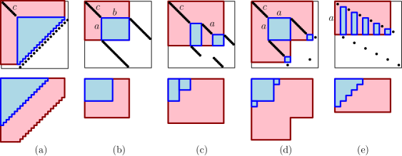
Refer to caption
Figure 6. The diagram (top) and skew shape (bottom) of the vexillary permutations 1c×wsuperscript1𝑐𝑤1^{c}\times w where w=w0,u(a,b),v(a)𝑤subscript𝑤0𝑢𝑎𝑏𝑣𝑎w=w_{0},u(a,b),v(a), w(a)𝑤𝑎w(a), and z(a)𝑧𝑎z(a) respectively.

5.3. 321321321-avoiding permutations

Recall from Section 2.2 that the diagram of a 321321321-avoiding permutation is, up to removing empty rows and columns and flipping columns, the diagram of a skew shape λ/μ𝜆𝜇\lambda/\mu. By Theorem 2.1(stating [BJS, Prop 2.2]) we can realize every skew shape λ/μ𝜆𝜇\lambda/\mu as the diagram of the 321321321-avoiding permutation given by the reduced word rw(λ/μ)rw𝜆𝜇\operatorname{rw}(\lambda/\mu). The map from shapes to permutations is outlined in Section 2.2.

Theorem 5.13.

Let w𝑤w be a 321321321-avoiding permutation. Then its diagram gives a skew shape λ/μ𝜆𝜇\lambda/\mu. Conversely, every skew shape λ/μ𝜆𝜇\lambda/\mu can be realized from the diagram of a 321321321-avoiding permutation w𝑤w. In both cases, we have:

Υw=1!r1rfλ/μ,subscriptΥ𝑤1subscript𝑟1subscript𝑟superscript𝑓𝜆𝜇{\small{\Upsilon}}_{w}\,=\,\frac{1}{\ell!}\,\hskip 1.70709ptr_{1}\hskip 1.70709pt\cdots\hskip 1.70709ptr_{\ell}\,f^{\lambda/\mu}\hskip 1.70709pt,

where =|λ/μ|𝜆𝜇\hskip 0.85355pt\ell=|\lambda/\mu|\hskip 0.85355pt and (r1,,r)subscript𝑟1subscript𝑟\hskip 0.85355pt(r_{1},\ldots,r_{\ell})\hskip 0.85355pt is a reduced word of w𝑤w.

Proof.

The fact that diagrams of 321321321-avoiding permutations yield skew shapes and its converse are explained in Section 2.2.

Assume that the 321321321-avoiding permutation has skew shape  skewsh(w)=λ/μskewsh𝑤𝜆𝜇\operatorname{skewsh}(w)=\lambda/\mu. The reduced words of a 321321321-avoiding permutation are obtained from one another by only using commutation relations sisj=sjsisubscript𝑠𝑖subscript𝑠𝑗subscript𝑠𝑗subscript𝑠𝑖s_{i}s_{j}=s_{j}s_{i} for |ij|>1𝑖𝑗1|i-j|>1 [BJS, Thm. 2.1]. Thus, all reduced words (r1,,r)subscript𝑟1subscript𝑟(r_{1},\ldots,r_{\ell}) of w𝑤w have the same product r1rsubscript𝑟1subscript𝑟\hskip 0.85355ptr_{1}\hskip 0.85355pt\cdots\hskip 0.85355ptr_{\ell}. Also, the number of reduced words of w𝑤w equals  fλ/μsuperscript𝑓𝜆𝜇f^{\lambda/\mu}, see [BJS, Cor. 2.1]. The result then follows by using these two facts and Macdonald’s identity (2.6). ∎

As an illustration we obtain permutations such that ΥwsubscriptΥ𝑤{\small{\Upsilon}}_{w} give double factorials and Euler numbers.

Corollary 5.14.

For the permutations w=2143(2n)(2n1)𝑤21432𝑛2𝑛1w=2143\cdots(2n)(2n-1) and w1atensor-product𝑤superscript1𝑎w\otimes 1^{a}, we have:

ΥwsubscriptΥ𝑤\displaystyle{\small{\Upsilon}}_{w} =(2n1)!!andΥw1aabsentdouble-factorial2𝑛1andsubscriptΥtensor-product𝑤superscript1𝑎\displaystyle\,=\,(2n-1)!!\qquad\text{and}\qquad{\small{\Upsilon}}_{w\hskip 0.85355pt\otimes\hskip 0.85355pt1^{a}} =Φ(2na)Φ(a)2n2Φ(2a)n[k=1n1Φ(2ka)Φ((2k+1)a)]2.absentΦ2𝑛𝑎Φsuperscript𝑎2𝑛2Φsuperscript2𝑎𝑛superscriptdelimited-[]superscriptsubscriptproduct𝑘1𝑛1Φ2𝑘𝑎Φ2𝑘1𝑎2\displaystyle\,=\,\hskip 0.85355pt\frac{\Phi(2na)\hskip 1.70709pt\Phi(a)^{2n-2}}{\Phi(2a)^{n}}\,\left[\hskip 1.70709pt\prod_{k=1}^{n-1}\frac{\Phi(2ka)}{\Phi\bigl{(}(2k+1)a\bigr{)}}\hskip 0.85355pt\right]^{2}\hskip 0.85355pt.
Proof.

The number of SYT of the diagonal shape δn+1/δnsubscript𝛿𝑛1subscript𝛿𝑛\delta_{n+1}/\delta_{n} is n!𝑛n!. By the construction from Theorem 2.1, from this shape we read off the reduced word

rw(δn+1/δn)=(1,3,5,,2n1),rwsubscript𝛿𝑛1subscript𝛿𝑛1352𝑛1\operatorname{rw}(\delta_{n+1}/\delta_{n})\hskip 1.70709pt=\hskip 1.70709pt(1,3,5,\ldots,2n-1)\hskip 0.85355pt,

defining the permutation w𝑤w. See Figure 8 for an example. The product of the entries of this reduced word is (2n1)!!double-factorial2𝑛1(2n-1)!!  The result then follows by Theorem 5.13. The second formula comes from the 321321321-avoiding permutation w1atensor-product𝑤superscript1𝑎w\otimes 1^{a} whose skew shape consists of n𝑛n disjoint a×a𝑎𝑎a\times a blocks. ∎

Let 𝖠𝗅𝗍(n)={σ(1)<σ(2)>σ(3)<σ(4)>}SSn𝖠𝗅𝗍𝑛𝜎1expectation𝜎2𝜎3expectation𝜎4subscriptSS𝑛\mathsf{Alt}(n)=\{\sigma(1)<\sigma(2)>\sigma(3)<\sigma(4)>\ldots\}\subset\SS_{n} be the set of alternating permutations. The number En=|𝖠𝗅𝗍(n)|subscript𝐸𝑛𝖠𝗅𝗍𝑛E_{n}=|\mathsf{Alt}(n)| is the n𝑛n-th Euler number (see [OEIS, A000111]), with the generating function

(5.4) n=0Enxnn!=tan(x)+sec(x).superscriptsubscript𝑛0subscript𝐸𝑛superscript𝑥𝑛𝑛𝑥𝑥\sum_{n=0}^{\infty}\hskip 1.70709ptE_{n}\hskip 1.70709pt\frac{x^{n}}{n!}\,\hskip 1.70709pt=\,\,\tan(x)\hskip 0.85355pt+\hskip 0.85355pt\sec(x)\hskip 0.85355pt.

Let x(n)𝑥𝑛x(n) be a permutation with reduced word corresponding to the zigzag shape

rw(δn+2/δn)=(2,1,4,3,,2n,2n1,2n+1).rwsubscript𝛿𝑛2subscript𝛿𝑛21432𝑛2𝑛12𝑛1\operatorname{rw}(\delta_{n+2}/\delta_{n})\hskip 1.70709pt=\hskip 1.70709pt(2,1,4,3,\ldots,2n,2n-1,2n+1)\hskip 0.85355pt.

Similarly, define y(n)𝑦𝑛y(n) and z(n)𝑧𝑛z(n) to be the permutations with reduced words corresponding to shapes  (n+1)2n(n1)2/δnsuperscript𝑛12𝑛𝑛12subscript𝛿𝑛(n+1)^{2}n(n-1)\ldots 2/\delta_{n}  and  (n+2)3(n+1)n3/δnsuperscript𝑛23𝑛1𝑛3subscript𝛿𝑛(n+2)^{3}(n+1)n\ldots 3/\delta_{n}, respectively.

Corollary 5.15.

For the permutations x(n)𝑥𝑛x(n), y(n)𝑦𝑛y(n), and z(n)𝑧𝑛z(n) defined above, we have:

Υx(n)=E2n+1,Υy(n)=n!E2n+12n,Υz(n)=(n+1)(2n+3)!E2n+12n!25n+1(22n+21).formulae-sequencesubscriptΥ𝑥𝑛subscript𝐸2𝑛1formulae-sequencesubscriptΥ𝑦𝑛𝑛subscript𝐸2𝑛1superscript2𝑛subscriptΥ𝑧𝑛𝑛12𝑛3superscriptsubscript𝐸2𝑛12𝑛superscript25𝑛1superscript22𝑛21{\small{\Upsilon}}_{x(n)}\hskip 1.70709pt=\hskip 1.70709ptE_{2n+1},\quad{\small{\Upsilon}}_{y(n)}\hskip 1.70709pt=\hskip 1.70709pt\frac{n!\hskip 1.70709ptE_{2n+1}}{2^{n}},\quad{\small{\Upsilon}}_{z(n)}\hskip 1.70709pt=\hskip 1.70709pt\frac{(n+1)\hskip 0.85355pt(2n+3)!\hskip 1.70709ptE_{2n+1}^{2}}{n!\hskip 1.70709pt2^{5n+1}\hskip 0.85355pt\bigl{(}2^{2n+2}-1\bigr{)}}.
Proof.

The number of SYT of the zigzag shape δn+2/δnsubscript𝛿𝑛2subscript𝛿𝑛\delta_{n+2}/\delta_{n} is given by the Euler number E2n+1subscript𝐸2𝑛1E_{2n+1}. By the construction from Theorem 2.1, from this shape we read off the reduced word

rw(δn+2/δn)=(2,1,4,3,,2n,2n1,2n+1),rwsubscript𝛿𝑛2subscript𝛿𝑛21432𝑛2𝑛12𝑛1\operatorname{rw}(\delta_{n+2}/\delta_{n})=(2,1,4,3,\ldots,2n,2n-1,2n+1),

defining the permutation x(n)𝑥𝑛x(n). The product of the entries of this reduced word is (2n+1)!2𝑛1(2n+1)!  The first equality then follows by Theorem 5.13.

The second and third equalities follow by a similar argument for the 333-zigzag and 555-zigzag shape, respectively, whose number of SYT is given by [BR, Thm. 1]. We omit the easy details. See Figure 8, 8 and 8 for examples. ∎

We also obtain a family of 321321321-avoiding permutations w𝑤w that yield the skew shapes from Section 4 with product Λ(a,b,c,d,e,f)Λ𝑎𝑏𝑐𝑑𝑒𝑓\Lambda(a,b,c,d,e,f). Then by theorems 4.1 and 5.13, for such permutations, ΥwsubscriptΥ𝑤{\small{\Upsilon}}_{w} is given by a product formula. We illustrate this for the cases Λ(a,a,a,a,a,0)Λ𝑎𝑎𝑎𝑎𝑎0\Lambda(a,a,a,a,a,0) and Λ(a,a,a,1,1,1)Λ𝑎𝑎𝑎111\Lambda(a,a,a,1,1,1). See Figure 8,8 for examples.

Refer to caption
Figure 7. The reduced words rw(λ/μ)rw𝜆𝜇\operatorname{rw}(\lambda/\mu) of the skew shapes δn+1/δnsubscript𝛿𝑛1subscript𝛿𝑛\delta_{n+1}/\delta_{n}, the zigzag δn+2/δnsubscript𝛿𝑛2subscript𝛿𝑛\delta_{n+2}/\delta_{n}, 333-zigzag, 555-zigzag, (3a)2a(2a)a/aasuperscript3𝑎2𝑎superscript2𝑎𝑎superscript𝑎𝑎(3a)^{2a}(2a)^{a}/a^{a}, and δ4a/aasubscript𝛿4𝑎superscript𝑎𝑎\delta_{4a}/a^{a}.

We now restate Corollary 1.5 in the notation above.

Corollary 5.16 (shape (3a)2a(2a)a/aasuperscript3𝑎2𝑎superscript2𝑎𝑎superscript𝑎𝑎\hskip 0.85355pt(3a)^{2a}(2a)^{a}/a^{a}).

For the permutation s(a):=3516241aassign𝑠𝑎tensor-product351624superscript1𝑎\hskip 0.85355pts(a):=351624\otimes 1^{a}, we have:

Υs(a)=Φ(a)5Φ(3a)2Φ(5a)Φ(2a)4Φ(4a)2.subscriptΥ𝑠𝑎Φsuperscript𝑎5Φsuperscript3𝑎2Φ5𝑎Φsuperscript2𝑎4Φsuperscript4𝑎2{\small{\Upsilon}}_{s(a)}\,=\,\frac{\Phi(a)^{5}\hskip 1.70709pt\Phi(3a)^{2}\hskip 1.70709pt\Phi(5a)}{\Phi(2a)^{4}\hskip 1.70709pt\Phi(4a)^{2}}\,.
Proof.

The reading word associated to the shape 322/1superscript32213^{2}2/1 is (2,1,4,3,2,5,4)2143254(2,1,4,3,2,5,4) which defines the permutation 351624351624351624. Similarly, the shape (3a)2a(2a)a/aasuperscript3𝑎2𝑎superscript2𝑎𝑎superscript𝑎𝑎\hskip 0.85355pt(3a)^{2a}(2a)^{a}/a^{a}  yields a reduced word  (r1,,r7a2)subscript𝑟1subscript𝑟7superscript𝑎2(r_{1},\ldots,r_{7a^{2}}), defining the 321321321-avoiding permutation  s(a)=3516241a𝑠𝑎tensor-product351624superscript1𝑎s(a)=351624\otimes 1^{a}. By Theorem 5.13, we have:

Υs(a)=r1r7a2(7a2)!f(3a)2a(2a)a/aa.subscriptΥ𝑠𝑎subscript𝑟1subscript𝑟7superscript𝑎27superscript𝑎2superscript𝑓superscript3𝑎2𝑎superscript2𝑎𝑎superscript𝑎𝑎{\small{\Upsilon}}_{s(a)}\,=\,\frac{r_{1}\cdots r_{7a^{2}}}{(7a^{2})!}\,f^{(3a)^{2a}(2a)^{a}/a^{a}}\,.

The result now follows by writing the product of the entries of the reduced word as

r1r7a2=Φ(3a)2Φ(6a)Φ(2a)2Φ(4a)2subscript𝑟1subscript𝑟7superscript𝑎2Φsuperscript3𝑎2Φ6𝑎Φsuperscript2𝑎2Φsuperscript4𝑎2r_{1}\cdots r_{7a^{2}}\,=\,\frac{\Phi(3a)^{2}\hskip 1.70709pt\Phi(6a)}{\Phi(2a)^{2}\hskip 1.70709pt\Phi(4a)^{2}}

(see Figure 7). Now use Corollary 1.1 to write the number of SYT as

(5.5) f(3a)2a(2a)a/aa=(7a2)!Φ(a)5Φ(5a)Φ(2a)2Φ(6a),superscript𝑓superscript3𝑎2𝑎superscript2𝑎𝑎superscript𝑎𝑎7superscript𝑎2Φsuperscript𝑎5Φ5𝑎Φsuperscript2𝑎2Φ6𝑎f^{(3a)^{2a}(2a)^{a}/a^{a}}\,=\,\frac{(7a^{2})!\,\Phi(a)^{5}\hskip 1.70709pt\Phi(5a)}{\Phi(2a)^{2}\hskip 1.70709pt\Phi(6a)}\,,

and the result follows. ∎

Corollary 5.17 (shape δ4a/aasubscript𝛿4𝑎superscript𝑎𝑎\hskip 0.85355pt\delta_{4a}/a^{a}).

Let t(a)𝑡𝑎t(a) be the permutation of size (8a2)8𝑎2(8a-2) obtained from the reading word of the skew shape δ4a/aasubscript𝛿4𝑎superscript𝑎𝑎\hskip 0.85355pt\delta_{4a}/a^{a}. Then:

Υt(a)=Φ(a)3Φ(3a)Φ(4a1)Φ(8a2)Ψ(a)Ψ(3a)Φ(2a)2Φ(3a1)Φ(5a1)Ψ(2a)2Ψ(4a)(8a2).subscriptΥ𝑡𝑎Φsuperscript𝑎3Φ3𝑎Φ4𝑎1Φ8𝑎2Ψ𝑎Ψ3𝑎Φsuperscript2𝑎2Φ3𝑎1Φ5𝑎1Ψsuperscript2𝑎2Ψ4𝑎8𝑎2{\small{\Upsilon}}_{t(a)}\,=\,\frac{\Phi(a)^{3}\hskip 1.70709pt\Phi(3a)\hskip 1.70709pt\Phi(4a-1)\hskip 1.70709pt\Phi(8a-2)\hskip 1.70709pt\cdot\hskip 1.70709pt\Psi(a)\hskip 1.70709pt\Psi(3a)}{\Phi(2a)^{2}\hskip 1.70709pt\Phi(3a-1)\hskip 1.70709pt\Phi(5a-1)\hskip 1.70709pt\cdot\hskip 1.70709pt\Psi(2a)^{2}\hskip 1.70709pt\Psi(4a)\hskip 1.70709pt\cdot\hskip 1.70709pt\gimel(8a-2)}\,.
Proof.

The reduced word rw(δ4a/aa)rwsubscript𝛿4𝑎superscript𝑎𝑎\operatorname{rw}(\delta_{4a}/a^{a}) defines the permutation t(a)𝑡𝑎t(a). By Theorem 5.13 we have:

Υt(a)=r1r!fδ4a+1/aa.subscriptΥ𝑡𝑎subscript𝑟1subscript𝑟superscript𝑓subscript𝛿4𝑎1superscript𝑎𝑎{\small{\Upsilon}}_{t(a)}\,=\,\frac{r_{1}\cdots r_{\ell}}{\ell!}\,f^{\delta_{4a+1}/a^{a}}.

We can write the product of the entries of the reduced word as

r1r2r=Φ(4a1)Φ(8a2)Φ(3a1)Φ(5a1)(8a2),subscript𝑟1subscript𝑟2subscript𝑟Φ4𝑎1Φ8𝑎2Φ3𝑎1Φ5𝑎18𝑎2r_{1}r_{2}\cdots r_{\ell}\,=\,\frac{\Phi(4a-1)\hskip 1.70709pt\Phi(8a-2)}{\Phi(3a-1)\hskip 1.70709pt\Phi(5a-1)\hskip 1.70709pt\gimel(8a-2)}\,,

(see Figure 7). On the other hand, Corollary 1.2 gives:

(5.6) fδ4a+1/aa=!Φ(a)3Φ(3a)Ψ(a)Ψ(3a)Φ(2a)2Ψ(2a)2Ψ(4a),superscript𝑓subscript𝛿4𝑎1superscript𝑎𝑎Φsuperscript𝑎3Φ3𝑎Ψ𝑎Ψ3𝑎Φsuperscript2𝑎2Ψsuperscript2𝑎2Ψ4𝑎f^{\delta_{4a+1}/a^{a}}\,=\,\frac{\ell!\hskip 1.70709pt\cdot\hskip 1.70709pt\Phi(a)^{3}\hskip 1.70709pt\Phi(3a)\hskip 1.70709pt\Psi(a)\hskip 1.70709pt\Psi(3a)}{\Phi(2a)^{2}\hskip 1.70709pt\Psi(2a)^{2}\hskip 1.70709pt\Psi(4a)}\,,

where =(4a2)a2binomial4𝑎2superscript𝑎2\hskip 0.85355pt\ell=\binom{4a}{2}-a^{2}. Combining these formulas, we obtain the result. ∎

Refer to caption
Refer to caption
Refer to caption
Refer to caption
Refer to caption
Refer to caption
Figure 8. The diagram of the 321321321-avoiding permutations  w=214365𝑤214365w=214365, x(3)=31527486𝑥331527486x(3)=31527486, y(3)𝑦3y(3), z(3)𝑧3z(3), s(2)=35162412𝑠2tensor-product351624superscript12s(2)=351624\otimes 1^{2} and t(2)𝑡2t(2), with skew shapes  δ4/δ3subscript𝛿4subscript𝛿3\delta_{4}/\delta_{3}, δ5/δ3subscript𝛿5subscript𝛿3\delta_{5}/\delta_{3}, 4232/δ3superscript4232subscript𝛿34^{2}32/\delta_{3}, 5343/δ3superscript5343subscript𝛿35^{3}43/\delta_{3}, 6442/22superscript64superscript42superscript226^{4}4^{2}/2^{2} and δ8/22subscript𝛿8superscript22\delta_{8}/2^{2} respectively.

5.4. Conjectural formula

The number of SYT of the skew shape of the vexillary permutation  1c×w(a)superscript1𝑐𝑤𝑎1^{c}\times w(a)  defined in (5.3) appears to have the following formula similar to Corollary 1.1 when a=b=d=e𝑎𝑏𝑑𝑒a=b=d=e.

Conjecture 5.18 (joint with C. Krattenthaler).

Let λ=(2a+c)c+a(a+c)a𝜆superscript2𝑎𝑐𝑐𝑎superscript𝑎𝑐𝑎\hskip 0.85355pt\lambda=(2a+c)^{c+a}(a+c)^{a}, μ=(a+1)aa11𝜇𝑎1superscript𝑎𝑎11\hskip 0.85355pt\mu=(a+1)a^{a-1}1. Then:

(5.7) fλ/μ=n!Φ(a)4Φ(c)Φ(4a+c)Φ(2a)2Φ(4a+2c)[a2((2a2+4ac+c2)2a2)4a21].superscript𝑓𝜆𝜇𝑛Φsuperscript𝑎4Φ𝑐Φ4𝑎𝑐Φsuperscript2𝑎2Φ4𝑎2𝑐delimited-[]superscript𝑎2superscript2superscript𝑎24𝑎𝑐superscript𝑐22superscript𝑎24superscript𝑎21f^{\lambda/\mu}\,=\,n!\,\hskip 1.70709pt\frac{\Phi(a)^{4}\hskip 1.70709pt\Phi(c)\hskip 1.70709pt\Phi(4a+c)}{\Phi(2a)^{2}\hskip 1.70709pt\Phi(4a+2c)}\,\left[\frac{a^{2}\hskip 0.85355pt\bigl{(}(2a^{2}+4ac+c^{2})^{2}-a^{2}\bigr{)}}{4a^{2}-1}\right]\hskip 0.85355pt.

where n=|λ/μ|=(2a+c)22a22𝑛𝜆𝜇superscript2𝑎𝑐22superscript𝑎22\hskip 0.85355ptn=|\lambda/\mu|=(2a+c)^{2}-2a^{2}-2.

Remark 5.19.

For a=c𝑎𝑐a=c, formula (5.7) for the number of SYT of shape (3a)2a(2a)a/(a+1)aa11superscript3𝑎2𝑎superscript2𝑎𝑎𝑎1superscript𝑎𝑎11(3a)^{2a}(2a)^{a}/(a+1)a^{a-1}1 is

(5.8) fλ/μ=n!Φ(a)5Φ(5a)Φ(2a)2Φ(6a)[(49a21)a44a21].superscript𝑓𝜆𝜇𝑛Φsuperscript𝑎5Φ5𝑎Φsuperscript2𝑎2Φ6𝑎delimited-[]49superscript𝑎21superscript𝑎44superscript𝑎21f^{\lambda/\mu}\,=\,n!\,\hskip 1.70709pt\frac{\Phi(a)^{5}\hskip 1.70709pt\Phi(5a)}{\Phi(2a)^{2}\hskip 1.70709pt\Phi(6a)}\,\left[\frac{(49a^{2}-1)\hskip 0.85355pta^{4}}{4a^{2}-1}\right]\hskip 0.85355pt.

This formula was suggested by Christian Krattenthaler,444Personal communication. based on computational data and was a precursor of the conjecture above.555Both Krattenthaler’s formula and Conjecture 5.18 were recently established in [KY]. Note the close resemblance of (5.8) and (5.5), which are the same up to a polynomial factor. This suggests that perhaps there is a common generalization.


6. Asymptotic applications

6.1. Number of SYT

In [MPP3], we prove that for a sequence  π¯={π(n)}¯𝜋superscript𝜋𝑛\overline{\pi}=\bigl{\{}\pi^{(n)}\bigr{\}}  of strongly stable skew shapes π(n)=λ(n)/μ(n)superscript𝜋𝑛superscript𝜆𝑛superscript𝜇𝑛\pi^{(n)}=\lambda^{(n)}/\mu^{(n)}, |π(n)|=nsuperscript𝜋𝑛𝑛\bigl{|}\pi^{(n)}\bigr{|}=n, we have:

()log|SYT(π(n))|=12nlogn+O(n).SYTsuperscript𝜋𝑛12𝑛𝑛𝑂𝑛(\ast)\qquad\log\,\bigl{|}\operatorname{{\rm SYT}}\bigl{(}\pi^{(n)}\bigr{)}\bigr{|}\,=\,\hskip 1.70709pt\frac{1}{2}\hskip 1.70709ptn\hskip 0.85355pt\log n\hskip 1.70709pt+\hskip 1.70709ptO(n)\hskip 0.85355pt.

Furthermore, we conjecture that

()log|SYT(π(n))|=12nlogn+cn+o(n),(\ast\ast)\qquad\log\,\bigl{|}\operatorname{{\rm SYT}}\bigl{(}\pi^{(n)}\bigr{)}\bigr{|}\,=\,\hskip 1.70709pt\frac{1}{2}\hskip 1.70709ptn\hskip 0.85355pt\log n\hskip 1.70709pt+\hskip 1.70709ptc\hskip 0.85355ptn\hskip 1.70709pt+\hskip 1.70709pto(n)\hskip 0.85355pt,

for some constant c=c(π¯)𝑐𝑐¯𝜋c=c(\overline{\pi}).666This conjecture was recently established in [MPT] Here by the strongly stable skew shape we mean a sharp convergence to the limit shape of the Young diagrams of π(n)superscript𝜋𝑛\pi^{(n)} under scaling 1/n1𝑛1/\sqrt{n}, as n𝑛n\to\infty; we refer to [MPP3] for details.777See [DF] for related results for other growth regimes.

Until this paper, the exact value of c(π¯)𝑐¯𝜋c(\overline{\pi}) was possible to compute only for the usual and shifted shapes. Here we have a new family of shapes where this is possible.

Theorem 6.1.

Fix α,β,γ,δ,ϵ0𝛼𝛽𝛾𝛿italic-ϵ0\alpha,\beta,\gamma,\delta,\epsilon\geq 0, m𝑚m\in\mathbb{N}, and let

π(n)=Λ(αn,βn,γn,δn,ϵn,m).superscript𝜋𝑛Λ𝛼𝑛𝛽𝑛𝛾𝑛𝛿𝑛italic-ϵ𝑛𝑚\pi^{(n)}\hskip 1.70709pt=\hskip 1.70709pt\Lambda\bigl{(}\lfloor\alpha n\rfloor,\lfloor\beta n\rfloor,\lfloor\gamma n\rfloor,\lfloor\delta n\rfloor,\lfloor\epsilon n\rfloor,m\bigr{)}\hskip 0.85355pt.

Then the asymptotic formula ()(\ast\ast) holds for some c=c(α,β,γ,δ,ϵ,m)𝑐𝑐𝛼𝛽𝛾𝛿italic-ϵ𝑚c=c(\alpha,\beta,\gamma,\delta,\epsilon,m).

The proof of the theorem is straightforward from the product formula in Theorem 4.1 and asymptotic formulas in §§\S2.10. We omit the details.

Example 6.2.

Let π=Λ(a,a,a,a,a,0)𝜋Λ𝑎𝑎𝑎𝑎𝑎0\pi=\Lambda(a,a,a,a,a,0). Then |π|=7a2𝜋7superscript𝑎2|\pi|=7a^{2} and by (5.5), we have:

logfπsuperscript𝑓𝜋\displaystyle\log\hskip 0.85355ptf^{\pi} =log(7a2)!Φ(a)5Φ(5a)Φ(2a)2Φ(6a)= 7a2loga+absent7superscript𝑎2Φsuperscript𝑎5Φ5𝑎Φsuperscript2𝑎2Φ6𝑎limit-from7superscript𝑎2𝑎\displaystyle=\ \log\,\frac{(7a^{2})!\,\hskip 1.70709pt\Phi(a)^{5}\hskip 1.70709pt\Phi(5a)}{\Phi(2a)^{2}\hskip 1.70709pt\Phi(6a)}\ =\ 7\hskip 0.85355pta^{2}\log a\ +
+(7222log218log3+252log5+7log7)a2+O(aloga),72222183252577superscript𝑎2𝑂𝑎𝑎\displaystyle\qquad+\left(\frac{7}{2}\hskip 1.70709pt-\hskip 1.70709pt22\hskip 0.85355pt\log 2\hskip 1.70709pt-\hskip 1.70709pt18\hskip 0.85355pt\log 3\hskip 1.70709pt+\hskip 1.70709pt\frac{25}{2}\hskip 1.70709pt\log 5\hskip 1.70709pt+\hskip 1.70709pt7\hskip 0.85355pt\log 7\right)a^{2}+\hskip 1.70709ptO(a\log a)\hskip 0.85355pt,

The sum in parentheses shifted by (7/2)log7727(7/2)\log 7 is the exact value of the constant c(1,1,1,1,1,0)𝑐111110c(1,1,1,1,1,0) as in the theorem.

6.2. Principal Schubert evaluations

In recent years, there has been some interest in the asymptotics of the principle evaluation Υw=𝔖w(1,,1)subscriptΥ𝑤subscript𝔖𝑤11\hskip 0.85355pt{\small{\Upsilon}}_{w}=\mathfrak{S}_{w}(1,\ldots,1). Notably, Stanley [Sta4] defined

u(n):=maxwSnΥwassign𝑢𝑛subscript𝑤subscript𝑆𝑛subscriptΥ𝑤u(n)\,:=\,\max_{w\in S_{n}}\hskip 1.70709pt{\small{\Upsilon}}_{w}

and observed that

()14lim infnlog2u(n)n2lim supnlog2u(n)n212.14subscriptlimit-infimum𝑛subscript2𝑢𝑛superscript𝑛2subscriptlimit-supremum𝑛subscript2𝑢𝑛superscript𝑛212(\divideontimes)\qquad\quad\frac{1}{4}\,\leq\,\liminf_{n\to\infty}\hskip 1.70709pt\frac{\log_{2}u(n)}{n^{2}}\,\leq\,\limsup_{n\to\infty}\hskip 1.70709pt\frac{\log_{2}u(n)}{n^{2}}\,\leq\,\frac{1}{2}\,.

Stanley also suggested existence of the limit of  1n2log2u(n)1superscript𝑛2subscript2𝑢𝑛\frac{1}{n^{2}}\log_{2}u(n), and that it is achieved on a certain “limit shape”. Below we apply our product formulas to obtain asymptotics of ΥwsubscriptΥ𝑤{\small{\Upsilon}}_{w} for some families of w𝑤w.

Proposition 6.3 (zigzag permutations).

For permutations wS2n𝑤subscript𝑆2𝑛w\in S_{2n} as in Corollary 5.14, x(n),y(n)S2n+2𝑥𝑛𝑦𝑛subscript𝑆2𝑛2x(n),y(n)\in S_{2n+2}, and z(n)S2n+4𝑧𝑛subscript𝑆2𝑛4z(n)\in S_{2n+4} as in Corollary 5.15, we have:   logΥw=Θ(nlogn)subscriptΥ𝑤Θ𝑛𝑛\log{\small{\Upsilon}}_{w}\hskip 0.85355pt=\hskip 0.85355pt\Theta(n\hskip 0.85355pt\log n),  logΥx(n)=Θ(nlogn)subscriptΥ𝑥𝑛Θ𝑛𝑛\log{\small{\Upsilon}}_{x(n)}\hskip 0.85355pt=\hskip 0.85355pt\Theta(n\hskip 0.85355pt\log n),  logΥy(n)=Θ(nlogn)subscriptΥ𝑦𝑛Θ𝑛𝑛\log{\small{\Upsilon}}_{y(n)}\hskip 0.85355pt=\hskip 0.85355pt\Theta(n\hskip 0.85355pt\log n),  and  logΥz(n)=Θ(nlogn)subscriptΥ𝑧𝑛Θ𝑛𝑛\log{\small{\Upsilon}}_{z(n)}\hskip 0.85355pt=\hskip 0.85355pt\Theta(n\hskip 0.85355pt\log n).

The proof follows immediately from the product formulas in corollaries as above, the asymptotics of (2n1)!!double-factorial2𝑛1(2n-1)!! and of the Euler numbers:

Enn!(2π)n4π(1+o(1))asn,formulae-sequencesimilar-tosubscript𝐸𝑛𝑛superscript2𝜋𝑛4𝜋1𝑜1as𝑛E_{n}\,\sim\,n!\hskip 1.70709pt\left(\frac{2}{\pi}\right)^{n}\frac{4}{\pi}\hskip 1.70709pt\bigl{(}1+o(1)\bigr{)}\quad\text{as}\ \ n\to\infty\hskip 0.85355pt,

(see e.g. [FS, Sta3]).

Proposition 6.4 (Macdonald permutations).

Consider permutations w0S2ksubscript𝑤0subscript𝑆2𝑘w_{0}\in S_{2k}, w^0=1k×w0S3ksubscript^𝑤0superscript1𝑘subscript𝑤0subscript𝑆3𝑘\widehat{w}_{0}=1^{k}\times w_{0}\in S_{3k} as in Corollary 5.8, u(k,k)S2k𝑢𝑘𝑘subscript𝑆2𝑘u(k,k)\in S_{2k}, u^(k,k)=1k×u(k,k)S3k^𝑢𝑘𝑘superscript1𝑘𝑢𝑘𝑘subscript𝑆3𝑘\widehat{u}(k,k)=1^{k}\times u(k,k)\in S_{3k} as in Corollary 5.9. Then we have:

logΥw^0 2(logC)k2,andlogΥu^(k,k)(logC)k2,whereC=39/226.formulae-sequencesimilar-tosubscriptΥsubscript^𝑤02𝐶superscript𝑘2andformulae-sequencesimilar-tosubscriptΥ^𝑢𝑘𝑘𝐶superscript𝑘2where𝐶superscript392superscript26\log{\small{\Upsilon}}_{\widehat{w}_{0}}\,\sim\,2\hskip 0.85355pt(\log C)\hskip 0.85355ptk^{2}\hskip 0.85355pt,\quad\text{and}\quad\log{\small{\Upsilon}}_{\widehat{u}(k,k)}\,\sim\,(\log C)\hskip 0.85355ptk^{2}\hskip 0.85355pt,\quad\text{where}\quad C\hskip 1.70709pt=\,\frac{3^{9/2}}{2^{6}}\,.

The proof is straightforward again and combines the corollaries in the proposition with the asymptotic formulas for Φ(n)Φ𝑛\Phi(n) and(n)𝑛~{}\gimel(n). In fact, the constant C𝐶C is the base of exponent in the symmetric case of the box formula (1.2) for |PP(n,n,n)|PP𝑛𝑛𝑛|\operatorname{PP}(n,n,n)|, see [OEIS, A008793].

From here, for n=3k𝑛3𝑘n=3k and w^0Snsubscript^𝑤0subscript𝑆𝑛\widehat{w}_{0}\in S_{n} as above, we have:

log2Υw^0n229log2C 0.251629asn=3k.formulae-sequencesubscript2subscriptΥsubscript^𝑤0superscript𝑛229subscript2𝐶0.251629as𝑛3𝑘\frac{\log_{2}{\small{\Upsilon}}_{\widehat{w}_{0}}}{n^{2}}\,\hskip 1.70709pt\to\,\hskip 1.70709pt\frac{2}{9}\hskip 1.70709pt\log_{2}C\,\approx\,0.251629\,\quad\text{as}\ \ n\hskip 0.85355pt=\hskip 0.85355pt3k\hskip 1.70709pt\to\hskip 0.85355pt\infty\hskip 0.85355pt.

This is a mild improvement over Stanley’s lower bound ()(\divideontimes).888In [MPP4] we improve this lower bound to about 0.2930.2930.293 and prove that this is maximal for principal Schubert evaluations of layered permutations.

Finally, for comparison, we obtain similar asymptotics for three more families of stable permutations, i.e. permutations whose diagrams have stable shape (cf. [MPP3]).

Proposition 6.5 (stable permutations).

Let v(a)=24131aS4a𝑣𝑎tensor-product2413superscript1𝑎subscript𝑆4𝑎v(a)=2413\otimes 1^{a}\in S_{4a} as in Corollary 5.11, s(a)=3516241aS6a𝑠𝑎tensor-product351624superscript1𝑎subscript𝑆6𝑎s(a)=351624\otimes 1^{a}\in S_{6a} as in Corollary 1.5, and t(a)S8a2𝑡𝑎subscript𝑆8𝑎2t(a)\in S_{8a-2} as in Corollary 5.17. Then we have:   logΥv(a)=Θ(a2)subscriptΥ𝑣𝑎Θsuperscript𝑎2\log{\small{\Upsilon}}_{v(a)}\hskip 0.85355pt=\hskip 0.85355pt\Theta(a^{2}),  logΥs(a)=Θ(a2)subscriptΥ𝑠𝑎Θsuperscript𝑎2\log{\small{\Upsilon}}_{s(a)}\hskip 0.85355pt=\hskip 0.85355pt\Theta(a^{2}),  and  logΥt(a)=Θ(a2)subscriptΥ𝑡𝑎Θsuperscript𝑎2\log{\small{\Upsilon}}_{t(a)}\hskip 0.85355pt=\hskip 0.85355pt\Theta(a^{2}).

We omit the proof which is again a straightforward calculation. To compare this with Stanley’s bound, take the following example:

log2Υs(a)n2(14log23+2572log25109) 0.091354asn=6a.formulae-sequencesubscript2subscriptΥ𝑠𝑎superscript𝑛214subscript232572subscript251090.091354as𝑛6𝑎\frac{\log_{2}{\small{\Upsilon}}_{s(a)}}{n^{2}}\,\hskip 1.70709pt\to\,\left(\frac{1}{4}\hskip 0.85355pt\log_{2}3\hskip 1.70709pt+\hskip 1.70709pt\frac{25}{72}\hskip 0.85355pt\log_{2}5\hskip 1.70709pt-\hskip 1.70709pt\frac{10}{9}\right)\,\approx\,0.091354\,\quad\text{as}\ \ n\hskip 0.85355pt=\hskip 0.85355pt6\hskip 0.85355pta\hskip 1.70709pt\to\hskip 0.85355pt\infty\hskip 0.85355pt.

This suggests that perhaps every family  {wSn}𝑤subscript𝑆𝑛\{w\in S_{n}\}  of stable permutations satisfies  Υw=expΘ(n2)subscriptΥ𝑤Θsuperscript𝑛2{\small{\Upsilon}}_{w}=\exp\Theta(n^{2}). On the other hand, as suggested by the exact computations in [MeS, Sta4], it is likely that that the maximum of ΥwsubscriptΥ𝑤{\small{\Upsilon}}_{w} is achieved on a smaller class of stable Richardson permutations.


7. Lozenge tilings with multivariate weights

In this section we study lozenge tilings of regions in the triangular grid. On a technical level, we show how the multivariate sums  Gλ/μ(𝐱|𝐲)subscript𝐺𝜆𝜇conditional𝐱𝐲G_{\lambda/\mu}({\bf x}\,|\,{\bf y})  appear in the context of lozenge tilings.

7.1. Combinatorics of lozenge tilings

Let us show how excited diagrams can be interpreted as lozenge tilings of certain shapes (plane partitions) with multivariate local weights. As a consequence, the multivariate sum Gλ/μ(𝐱|𝐲)subscript𝐺𝜆𝜇conditional𝐱𝐲G_{\lambda/\mu}({\bf x}\,|\,{\bf y}) of excited diagrams is a partition function of such lozenge tilings, and by Lemma 3.4 and the definition of factorial Schur functions it can be computed as a determinant.
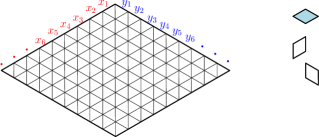
Refer to caption
Figure 9. Triangular grid in the plane with axes x and y. The grid is tiled with three types of lozenges. Horizontal lozenges at position (i,j)𝑖𝑗(i,j) have a weight xiyjsubscript𝑥𝑖subscript𝑦𝑗x_{i}-y_{j} (see Figure 10).

Consider the triangular grid in the plane where we identify two of the axes as x𝑥x and y𝑦y, see Figure 9. Adjacent triangles can be paired into lozenges, which can tile certain prescribed regions in the plane. The lozenges whose long axis is horizontal, are called horizontal lozenges, and are colored in blue in the picture. Each of these lozenges is assigned a local weight, depending on its position with respect to the x𝑥x and y𝑦y axes. More precisely, the weight of the lozenge at position (i,j)𝑖𝑗(i,j), is defined to be  (xiyj)subscript𝑥𝑖subscript𝑦𝑗(x_{i}-y_{j}). Let ΓΓ\Gamma be a region in the plane, and let T𝑇T be a tiling of ΓΓ\Gamma (no holes, no overlaps). Let  𝐡𝐥(T)𝐡𝐥𝑇{{\mathbf{\hskip 0.56917pthl}}}(T)  denote the set of horizontal lozenges ([Uncaptioned image]) of T𝑇T, and let

(7.1) wt(T):=(i,j)𝐡𝐥(T)(xiyj)assignwt𝑇subscriptproduct𝑖𝑗𝐡𝐥𝑇subscript𝑥𝑖subscript𝑦𝑗\operatorname{wt}(T)\,:=\,\prod_{(i,j)\hskip 0.85355pt\in\hskip 0.85355pt{{\mathbf{\hskip 0.56917pthl}}}(T)}\hskip 1.70709pt(x_{i}-y_{j})

be the weight of the tiling T𝑇T.

For a partition μ𝜇\mu and an integer d𝑑d, consider plane partitions of base μ𝜇\mu and height at most d𝑑d, these correspond to the set of tilings Ωμ,dsubscriptΩ𝜇𝑑\Omega_{\mu,d} of the plane in the region whose lower side is given by μ𝜇\mu, and the rest is bounded by the top 4 sides of a hexagon of vertical side length d𝑑d. Given a skew partition λ/μ𝜆𝜇\lambda/\mu, let  Ωμ(λ)subscriptΩ𝜇𝜆\Omega_{\mu}(\lambda)  be the set of lozenge tilings TΩμ,d𝑇subscriptΩ𝜇𝑑T\in\Omega_{\mu,d}, d=max{f1(λ/μ)1,f(μ)(λ/μ)(μ)}𝑑superscriptsubscript𝑓1𝜆𝜇1superscriptsubscript𝑓𝜇𝜆𝜇𝜇d=\max\{f_{1}^{(\lambda/\mu)}-1,f_{\ell(\mu)}^{(\lambda/\mu)}-\ell(\mu)\}, such that on each vertical diagonal ij=k𝑖𝑗𝑘i-j=k there are no horizontal lozenges in T𝑇T with coordinates (i,j)𝑖𝑗(i,j) for j>λi𝑗subscript𝜆𝑖j>\lambda_{i}. The hook weight of T𝑇T at position (i,j)𝑖𝑗(i,j) is obtained from wt(T)wt𝑇\operatorname{wt}(T) by evaluating  xi=(λii+1)subscript𝑥𝑖subscript𝜆𝑖𝑖1x_{i}=(\lambda_{i}-i+1)  and  yj=(λj+j)subscript𝑦𝑗subscriptsuperscript𝜆𝑗𝑗y_{j}=(-\lambda^{\prime}_{j}+j) :

(7.2) wtλ(T):=(i,j)𝐡𝐥(T)(λii+λjj+1).assignsubscriptwt𝜆𝑇subscriptproduct𝑖𝑗𝐡𝐥𝑇subscript𝜆𝑖𝑖subscriptsuperscript𝜆𝑗𝑗1\operatorname{wt}_{\lambda}(T)\,:=\,\prod_{(i,j)\hskip 0.85355pt\in\hskip 0.85355pt{{\mathbf{\hskip 0.56917pthl}}}(T)}(\lambda_{i}-i+\lambda^{\prime}_{j}-j+1)\hskip 1.70709pt.

We define the following map between excited diagrams and lozenge tilings of base μ𝜇\mu. Let D(λ/μ)𝐷𝜆𝜇D\in\mathcal{E}(\lambda/\mu), then define τ(D):=Tassign𝜏𝐷𝑇\tau(D):=T to be the tiling T𝑇T with base μ𝜇\mu, such that if box (i,j)D𝑖𝑗𝐷(i,j)\in D, then T𝑇T has a horizontal lozenge in position (i,j)𝑖𝑗(i,j) in the coordinates defined above. See Figure 10 for an example of τ𝜏\tau.

Example 7.1.

There are five lozenge tilings in Ω21(332)subscriptΩ21332\Omega_{21}(332) corresponding to excited diagrams from Example 2.2 :

[Uncaptioned image]
Theorem 7.2.

The map τ𝜏\tau is a bijection between excited diagrams (λ/μ)𝜆𝜇\mathcal{E}(\lambda/\mu) and lozenge tilings Ωμ(λ)subscriptΩ𝜇𝜆\Omega_{\mu}(\lambda).

Proof.

We first interpret the excited diagram D𝐷D as a plane partition P𝑃P of shape μ𝜇\mu (and nonpositive entries) under Pi,j=ri,j+isubscript𝑃𝑖𝑗subscript𝑟𝑖𝑗𝑖P_{i,j}=-r_{i,j}+i, alternatively a skew RPP Pi,j=ri,jisubscriptsuperscript𝑃𝑖𝑗subscript𝑟𝑖𝑗𝑖P^{\prime}_{i,j}=r_{i,j}-i, where ri,jsubscript𝑟𝑖𝑗r_{i,j} is the row number of the final position of box (i,j)𝑖𝑗(i,j) of μ𝜇\mu after it has been moved under the excited moves from μ𝜇\mu to D𝐷D. Next, P𝑃P corresponds to a lozenge tiling in the obvious way, where we set level 0 to be the top z𝑧z-plane and the horizontal lozenges are moved down to the heights given by Pi,jsubscript𝑃𝑖𝑗P_{i,j}. The condition D[λ]𝐷delimited-[]𝜆D\subset[\lambda] is equivalent to the condition that the boxes on diagonal ij=k𝑖𝑗𝑘i-j=k cannot move beyond the intersection of this diagonal and λ𝜆\lambda, so that the coordinates of a horizontal lozenge (i,j)𝑖𝑗(i,j) must satisfy jλi𝑗subscript𝜆𝑖j\leq\lambda_{i}. Finally, note that excited moves correspond to flips on lozenge tilings, see e.g. [Thu]. Since the starting excited diagram D=[μ]𝐷delimited-[]𝜇D=[\mu] corresponds to top-adjusted horizontal lozenges whose complement can be tiled by non-horizontal lozenges, the same holds for all D(λ/μ)𝐷𝜆𝜇D\in\mathcal{E}(\lambda/\mu). This implies that τ𝜏\tau is the desired bijection. ∎

From the map τ𝜏\tau, adding the corresponding weight of the horizontal lozenges, we obtain the following result.

Corollary 7.3.

For a skew shape λ/μ𝜆𝜇\lambda/\mu, we have

Gλ/μ(𝐱|𝐲)=TΩμ(λ)(i,j)𝐡𝐥(T)(xiyj).subscript𝐺𝜆𝜇conditional𝐱𝐲subscript𝑇subscriptΩ𝜇𝜆subscriptproduct𝑖𝑗𝐡𝐥𝑇subscript𝑥𝑖subscript𝑦𝑗G_{\lambda/\mu}({\bf x}\,|\,{\bf y})\,=\,\sum_{T\in\Omega_{\mu}(\lambda)}\,\prod_{(i,j)\in{{\mathbf{\hskip 0.56917pthl}}}(T)}\hskip 1.70709pt(x_{i}-y_{j})\hskip 1.70709pt.

As in the introduction, denote by  H(a,b,c)H𝑎𝑏𝑐\operatorname{H}(a,b,c)  the  a×b×c×a×b×cdelimited-⟨⟩𝑎𝑏𝑐𝑎𝑏𝑐\langle a\times b\times c\times a\times b\times c\rangle  hexagon with base a×b𝑎𝑏a\times b and height c𝑐c. Denote by  𝒯abcsubscript𝒯𝑎𝑏𝑐\mathcal{T}_{abc}  the set of lozenge tilings of  H(a,b,c)H𝑎𝑏𝑐\operatorname{H}(a,b,c)  weighted as in (7.1).

Corollary 7.4.

For all  a,b,c,d,e𝑎𝑏𝑐𝑑𝑒a,b,c,d,e\in\mathbb{N}, we have

(7.3) T𝒯abc(i,j)𝐡𝐥(T)(kij)=Φ(a+b+c+d+e)Φ(c+d+e)Φ(a+b+c)Φ(a)Φ(b)Φ(c)Φ(a+c+d+e)Φ(b+c+d+e)Φ(a+b)Φ(b+c)Φ(a+c),subscript𝑇subscript𝒯𝑎𝑏𝑐subscriptproduct𝑖𝑗𝐡𝐥𝑇𝑘𝑖𝑗Φ𝑎𝑏𝑐𝑑𝑒Φ𝑐𝑑𝑒Φ𝑎𝑏𝑐Φ𝑎Φ𝑏Φ𝑐Φ𝑎𝑐𝑑𝑒Φ𝑏𝑐𝑑𝑒Φ𝑎𝑏Φ𝑏𝑐Φ𝑎𝑐\sum_{T\in\mathcal{T}_{abc}}\hskip 1.70709pt\prod_{(i,j)\in{{\mathbf{\hskip 0.56917pthl}}}(T)}\hskip 1.70709pt(k-i-j)\,=\,\frac{\Phi(a+b+c+d+e)\hskip 1.70709pt\Phi(c+d+e)\Phi(a+b+c)\hskip 1.70709pt\Phi(a)\hskip 1.70709pt\Phi(b)\hskip 1.70709pt\Phi(c)}{\Phi(a+c+d+e)\hskip 1.70709pt\Phi(b+c+d+e)\hskip 1.70709pt\Phi(a+b)\hskip 1.70709pt\Phi(b+c)\hskip 1.70709pt\Phi(a+c)}\,,

where k=a+b+2c+d+e+1𝑘𝑎𝑏2𝑐𝑑𝑒1k=a+b+2c+d+e+1.

First proof.

By Corollary 7.3 and 3.14 we have that

T𝒯abc(i,j)𝐡𝐥(T)(xiyj)=S((b+c)a+c/0cba)(i,j)S(xiyj).subscript𝑇subscript𝒯𝑎𝑏𝑐subscriptproduct𝑖𝑗𝐡𝐥𝑇subscript𝑥𝑖subscript𝑦𝑗subscript𝑆superscriptsuperscript𝑏𝑐𝑎𝑐superscript0𝑐superscript𝑏𝑎subscriptproduct𝑖𝑗𝑆subscript𝑥𝑖subscript𝑦𝑗\sum_{T\in\mathcal{T}_{abc}}\,\prod_{(i,j)\in{{\mathbf{\hskip 0.56917pthl}}}(T)}\hskip 1.70709pt(x_{i}-y_{j})\,=\,\,\sum_{S\hskip 0.85355pt\in\hskip 0.85355pt\mathcal{E}^{\nearrow}\bigl{(}(b+c)^{a+c}/0^{c}b^{a}\bigr{)}}\prod_{(i,j)\in S}(x_{i}-y_{j})\hskip 0.85355pt.

Next we evaluate xi=kisubscript𝑥𝑖𝑘𝑖x_{i}=k-i and yj=jsubscript𝑦𝑗𝑗y_{j}=j to obtain the hook weight (kij)𝑘𝑖𝑗(k-i-j) for each horizontal lozenge at position (i,j)𝑖𝑗(i,j). Note that this hook weight is constant when (i+j)𝑖𝑗(i+j) is constant. Thus, each NE-excited diagram on the RHS above has the same contribution to the sum. Therefore, the product in the RHS is given by:

(i,j)S(kij)=(i,j)(b+c)a+c/0cba(kij)=Φ(a+b+c+d+e)Φ(c+d+e)Φ(a+c+d+e)Φ(b+c+d+e).subscriptproduct𝑖𝑗𝑆𝑘𝑖𝑗subscriptproduct𝑖𝑗superscript𝑏𝑐𝑎𝑐superscript0𝑐superscript𝑏𝑎𝑘𝑖𝑗Φ𝑎𝑏𝑐𝑑𝑒Φ𝑐𝑑𝑒Φ𝑎𝑐𝑑𝑒Φ𝑏𝑐𝑑𝑒\prod_{(i,j)\in S}(k-i-j)\,=\prod_{(i,j)\in(b+c)^{a+c}/0^{c}b^{a}}(k-i-j)\,=\,\frac{\Phi(a+b+c+d+e)\hskip 1.70709pt\Phi(c+d+e)}{\Phi(a+c+d+e)\hskip 1.70709pt\Phi(b+c+d+e)}\,.

Lastly, the number of excited diagrams is given by (1.2). ∎

Second proof.

Alternatively, by Corollary 7.3 and Lemma 4.6,

T𝒯abc(i,j)𝐡𝐥(T)(kij)=D(λ/μ)(i,j)Dhλ(i,j),subscript𝑇subscript𝒯𝑎𝑏𝑐subscriptproduct𝑖𝑗𝐡𝐥𝑇𝑘𝑖𝑗subscript𝐷𝜆𝜇subscriptproduct𝑖𝑗𝐷subscript𝜆𝑖𝑗\sum_{T\in\mathcal{T}_{abc}}\,\prod_{(i,j)\in{{\mathbf{\hskip 0.56917pthl}}}(T)}\hskip 1.70709pt(k-i-j)\,=\,\sum_{D\in\mathcal{E}(\lambda/\mu)}\hskip 1.70709pt\prod_{(i,j)\in D}\hskip 1.70709pth_{\lambda}(i,j),

where λ/μ=Λ(a,b,c,d,e,0)𝜆𝜇Λ𝑎𝑏𝑐𝑑𝑒0\lambda/\mu=\Lambda(a,b,c,d,e,0). By (NHLF), the RHS is equal to

1n!fΛ(a,b,c,d,e,0)(i,j)λhλ(i,j).1𝑛superscript𝑓Λ𝑎𝑏𝑐𝑑𝑒0subscriptproduct𝑖𝑗𝜆subscript𝜆𝑖𝑗\frac{1}{n!}\hskip 1.70709ptf^{\Lambda(a,b,c,d,e,0)}\hskip 1.70709pt\prod_{(i,j)\in\lambda}h_{\lambda}(i,j)\hskip 1.70709pt.

The result then follows form the product formula for fΛ(a,b,c,d,e,0)superscript𝑓Λ𝑎𝑏𝑐𝑑𝑒0f^{\Lambda(a,b,c,d,e,0)} from Corollary 1.1 and by taking the product of the hooks in λ𝜆\lambda. ∎

Refer to caption
Figure 10. Left: the correspondence between excited diagrams with inner partition μ=32𝜇32\mu=32, lozenge tilings with base μ𝜇\mu, and solid partitions. Right: the x𝑥x and y𝑦y coordinates giving local weights to horizontal lozenges. The highlighted horizontal lozenge has weight  (x3y5)subscript𝑥3subscript𝑦5(x_{3}-y_{5}).

7.2. Determinantal formulas for weighted lozenge tilings

Next, we give determinantal formulas for certain multivariate sums of lozenge tilings in Ωμ(λ)subscriptΩ𝜇𝜆\Omega_{\mu}(\lambda) and in Ωμ,dsubscriptΩ𝜇𝑑\Omega_{\mu,d}. Recall that Δ(𝐱)Δ𝐱\Delta({\bf x}) denotes the Vandermonde determinant.

Theorem 7.5.

Let λ/μ𝜆𝜇\lambda/\mu be a skew shape, and d𝑑d a sufficiently large positive integer, so that λ/μd×(d+μ1)𝜆𝜇𝑑𝑑subscript𝜇1\lambda/\mu\subset d\times(d+\mu_{1}). Let d=d+(μ)superscript𝑑𝑑𝜇d^{\prime}=d+\ell(\mu) and n:=d+d+μ1assign𝑛superscript𝑑𝑑subscript𝜇1n:=d^{\prime}+d+\mu_{1}. Then:

TΩμ(λ)wt(T)=det[(xiy1)(xiyμj+Ljj1)(xixd)(xixLj)]i,j=1nΔ(𝐱)1,subscript𝑇subscriptΩ𝜇𝜆wt𝑇superscriptsubscriptdelimited-[]subscript𝑥𝑖subscript𝑦1subscript𝑥𝑖subscript𝑦subscript𝜇𝑗subscript𝐿𝑗𝑗1subscript𝑥𝑖subscript𝑥superscript𝑑subscript𝑥𝑖subscript𝑥subscript𝐿𝑗𝑖𝑗1𝑛Δsuperscript𝐱1\displaystyle\sum_{T\in\Omega_{\mu}(\lambda)}\operatorname{wt}(T)\,=\,\det\bigl{[}(x_{i}-y_{1})\cdots(x_{i}-y_{\mu_{j}+L_{j}-j-1})(x_{i}-x_{d^{\prime}})\cdots(x_{i}-x_{L_{j}})\bigr{]}_{i,j=1}^{n}\Delta({\bf x})^{-1}\,,

where the sum is over lozenge tilings T𝑇T with base μ𝜇\mu and height d𝑑d, and

Lj:=min{k:λkk+1μjj}.assignsubscript𝐿𝑗:𝑘subscript𝜆𝑘𝑘1subscript𝜇𝑗𝑗L_{j}\hskip 1.70709pt:=\hskip 1.70709pt\min\{k:\lambda_{k}-k+1\leq\mu_{j}-j\}.
Proof.

We use Corollary 7.3 to rewrite the LHS above as the sum Gλ/μ(𝐱|𝐲)subscript𝐺𝜆𝜇conditional𝐱𝐲G_{\lambda/\mu}({\bf x}\,|\,{\bf y}) over excited diagrams. We then use Lemma 3.4 to write this sum as an evaluation of the factorial Schur function sμ(d)(𝐱|𝐳(λ))superscriptsubscript𝑠𝜇superscript𝑑conditional𝐱superscript𝐳𝜆s_{\mu}^{(d^{\prime})}({\bf x}\,|\,{\bf z^{(\lambda)}}) with zλi+(d+1i)=xisubscript𝑧subscript𝜆𝑖superscript𝑑1𝑖subscript𝑥𝑖z_{\lambda_{i}+(d^{\prime}+1-i)}=x_{i} and zd+jλj=yjsubscript𝑧superscript𝑑𝑗subscriptsuperscript𝜆𝑗subscript𝑦𝑗z_{d^{\prime}+j-\lambda^{\prime}_{j}}=y_{j}. Next, we evaluate this factorial Schur function via (2.3) as a determinant of terms (xiz1)(xizμj+dj)subscript𝑥𝑖subscript𝑧1subscript𝑥𝑖subscript𝑧subscript𝜇𝑗superscript𝑑𝑗(x_{i}-z_{1})\cdots(x_{i}-z_{\mu_{j}+d^{\prime}-j}). We note that {z1,,zμj+dj}={y1,,yμj+Lj1,xd,,xL}subscript𝑧1subscript𝑧subscript𝜇𝑗superscript𝑑𝑗subscript𝑦1subscript𝑦subscript𝜇𝑗𝐿𝑗1subscript𝑥superscript𝑑subscript𝑥𝐿\{z_{1},\ldots,z_{\mu_{j}+d^{\prime}-j}\}=\{y_{1},\ldots,y_{\mu_{j}+L-j-1},x_{d^{\prime}},\ldots,x_{L}\}, where L𝐿L gives the smallest index of z𝑧z which is at most μj+djsubscript𝜇𝑗superscript𝑑𝑗\mu_{j}+d^{\prime}-j and evaluates to x𝑥x. In other words, we must have  λL+(d+1L)μj+djsubscript𝜆𝐿superscript𝑑1𝐿subscript𝜇𝑗superscript𝑑𝑗\lambda_{L}+(d^{\prime}+1-L)\leq\mu_{j}+d^{\prime}-j. ∎

Theorem 7.6.

Consider lozenge tilings with base μ𝜇\mu and height d𝑑d. Then we have:

TΩμ,dwt(T)=det[Ai,j(μ,d)]i,j=1d+(μ),subscript𝑇subscriptΩ𝜇𝑑wt𝑇superscriptsubscriptdelimited-[]subscript𝐴𝑖𝑗𝜇𝑑𝑖𝑗1𝑑𝜇\sum_{T\in\Omega_{\mu,d}}\operatorname{wt}(T)\,=\,\det\bigl{[}A_{i,j}(\mu,d)\bigr{]}_{i,j=1}^{d+\ell(\mu)}\hskip 1.70709pt,

where

Ai,j(μ,d)={(xiy1)(xiyd+(μ)j)(xixi+1)1(xixd+(μ))1 if j>(μ),(xiy1)(xiyμj+d)(xixi+1)1(xixd+j)1 if id<j(μ),0 if jid.subscript𝐴𝑖𝑗𝜇𝑑casessubscript𝑥𝑖subscript𝑦1subscript𝑥𝑖subscript𝑦𝑑𝜇𝑗superscriptsubscript𝑥𝑖subscript𝑥𝑖11superscriptsubscript𝑥𝑖subscript𝑥𝑑𝜇1 if 𝑗𝜇subscript𝑥𝑖subscript𝑦1subscript𝑥𝑖subscript𝑦subscript𝜇𝑗𝑑superscriptsubscript𝑥𝑖subscript𝑥𝑖11superscriptsubscript𝑥𝑖subscript𝑥𝑑𝑗1 if 𝑖𝑑𝑗𝜇0 if 𝑗𝑖𝑑A_{i,j}(\mu,d)={\small\begin{cases}(x_{i}-y_{1})\cdots(x_{i}-y_{d+\ell(\mu)-j})(x_{i}-x_{i+1})^{-1}\cdots(x_{i}-x_{d+\ell(\mu)})^{-1}&\text{ if }\ j>\ell(\mu),\\ (x_{i}-y_{1})\cdots(x_{i}-y_{\mu_{j}+d})(x_{i}-x_{i+1})^{-1}\cdots(x_{i}-x_{d+j})^{-1}&\text{ if }\ i-d<j\leq\ell(\mu),\\ 0&\text{ if }\ j\leq i-d.\\ \end{cases}}
Proof.

In Theorem 7.5 we set λ=(μ1+d)d(μ+d)𝜆superscriptsubscript𝜇1𝑑𝑑𝜇𝑑\lambda=(\mu_{1}+d)^{d}(\mu+d), where μ+d𝜇𝑑\mu+d means adding d𝑑d to each part of the partition μ𝜇\mu. In other words, λ𝜆\lambda has the same border as μ𝜇\mu, but endpoints shifted by d𝑑d on both axes. By the bijection τ𝜏\tau from Theorem 7.2, it follows that Ωμ(λ)subscriptΩ𝜇𝜆\Omega_{\mu}(\lambda) correspond to (λ/μ)𝜆𝜇\mathcal{E}(\lambda/\mu), where the height of the lozenges is determined by how far along the diagonals the excited boxes move. By construction of λ𝜆\lambda, each diagonal has length d𝑑d between μ𝜇\mu and the border, so Ωμ(λ)=Ωμ,dsubscriptΩ𝜇𝜆subscriptΩ𝜇𝑑\Omega_{\mu}(\lambda)=\Omega_{\mu,d}.

We apply Theorem 7.5 with the given λ/μ𝜆𝜇\lambda/\mu and d𝑑d. We now plug in the value for λ𝜆\lambda in terms of μ𝜇\mu: λk+d=μk+dsubscript𝜆𝑘𝑑subscript𝜇𝑘𝑑\lambda_{k+d}=\mu_{k}+d for k(μ)𝑘𝜇k\leq\ell(\mu) and λk=d+μ1subscript𝜆𝑘𝑑subscript𝜇1\lambda_{k}=d+\mu_{1} for kd𝑘𝑑k\leq d. If kd𝑘𝑑k\leq d, then for all 1j(μ)1𝑗𝜇1\leq j\leq\ell(\mu) we have λk+1k=d+μ1+1k>μ11μjjsubscript𝜆𝑘1𝑘𝑑subscript𝜇11𝑘subscript𝜇11subscript𝜇𝑗𝑗\lambda_{k}+1-k=d+\mu_{1}+1-k>\mu_{1}-1\geq\mu_{j}-j. If k>d𝑘𝑑k>d, then λk+1k=μkd+1+dk=μi+1isubscript𝜆𝑘1𝑘subscript𝜇𝑘𝑑1𝑑𝑘subscript𝜇superscript𝑖1superscript𝑖\lambda_{k}+1-k=\mu_{k-d}+1+d-k=\mu_{i^{\prime}}+1-i^{\prime}, where i=kdsuperscript𝑖𝑘𝑑i^{\prime}=k-d. Then we see that for j(μ)𝑗𝜇j\leq\ell(\mu) we have Lj=min{k:λk+1kμjj}=d+min{i:μi+1iμjj}=d+j+1subscript𝐿𝑗:𝑘subscript𝜆𝑘1𝑘subscript𝜇𝑗𝑗𝑑:superscript𝑖subscript𝜇superscript𝑖1superscript𝑖subscript𝜇𝑗𝑗𝑑𝑗1L_{j}=\min\{k:\lambda_{k}+1-k\leq\mu_{j}-j\}=d+\min\{i^{\prime}:\mu_{i^{\prime}}+1-i^{\prime}\leq\mu_{j}-j\}=d+j+1. For j>(μ)𝑗𝜇j>\ell(\mu), we must have Lj=d+(μ)+1subscript𝐿𝑗𝑑𝜇1L_{j}=d+\ell(\mu)+1 and there are no (xixd)subscript𝑥𝑖subscript𝑥superscript𝑑(x_{i}-x_{d^{\prime}})\cdots terms. Finally, we observe that Δ(𝐱)=i(xixi+1)(xixd)Δ𝐱subscriptproduct𝑖subscript𝑥𝑖subscript𝑥𝑖1subscript𝑥𝑖subscript𝑥superscript𝑑\Delta({\bf x})=\prod_{i}(x_{i}-x_{i+1})\cdots(x_{i}-x_{d^{\prime}}) and divide each entry on line i𝑖i by the corresponding product (xixi+1)subscript𝑥𝑖subscript𝑥𝑖1(x_{i}-x_{i+1})\cdots. ∎

Corollary 7.7.

Consider lozenge tilings with base μ𝜇\mu, such that (μ)=𝜇\ell(\mu)=\ell and height d𝑑d, such that horizontal lozenges at position (i,j)𝑖𝑗(i,j) have weight xisubscript𝑥𝑖x_{i}. Then we have the following formula for the partition function:

TΩμ,d(i,j)𝐡𝐥(T)xi=det[Bi,j]i,j=1+d,subscript𝑇subscriptΩ𝜇𝑑subscriptproduct𝑖𝑗𝐡𝐥𝑇subscript𝑥𝑖superscriptsubscriptdelimited-[]subscript𝐵𝑖𝑗𝑖𝑗1𝑑\sum_{T\in\Omega_{\mu,d}}\prod_{(i,j)\in{{\mathbf{\hskip 0.56917pthl}}}(T)}x_{i}\,\hskip 1.70709pt=\,\det\bigl{[}B_{i,j}\bigr{]}_{i,j=1}^{\ell+d}\,,

where

Bi,j={xid+j(xixi+1)1(xixd+)1 if j>(μ),xiμj+d(xixi+1)1(xixd+j)1 if id<j,0 if jid.subscript𝐵𝑖𝑗casessuperscriptsubscript𝑥𝑖𝑑𝑗superscriptsubscript𝑥𝑖subscript𝑥𝑖11superscriptsubscript𝑥𝑖subscript𝑥𝑑1 if 𝑗𝜇superscriptsubscript𝑥𝑖subscript𝜇𝑗𝑑superscriptsubscript𝑥𝑖subscript𝑥𝑖11superscriptsubscript𝑥𝑖subscript𝑥𝑑𝑗1 if 𝑖𝑑𝑗0 if 𝑗𝑖𝑑\displaystyle B_{i,j}=\begin{cases}x_{i}^{d+\ell-j}(x_{i}-x_{i+1})^{-1}\cdots(x_{i}-x_{d+\ell})^{-1}&\text{ if }\ j>\ell(\mu),\\ x_{i}^{\mu_{j}+d}(x_{i}-x_{i+1})^{-1}\cdots(x_{i}-x_{d+j})^{-1}&\text{ if }\ i-d<j\leq\ell,\\ 0&\text{ if }\ j\leq i-d.\\ \end{cases}
Proof.

We the apply Theorem 7.6 with yj=0subscript𝑦𝑗0y_{j}=0 and d=d+superscript𝑑𝑑d^{\prime}=d+\ell an obtain the result.∎

As a byproduct of our calculations we obtain the following determinant formula given in [Kra1, Thm. 6.1] with α=β=0𝛼𝛽0\alpha=\beta=0. To state this formula we use the standard notation of the q𝑞q-Pochhammer symbol (a;q)m:=(1a)(1aq)(1aqm1)assignsubscript𝑎𝑞𝑚1𝑎1𝑎𝑞1𝑎superscript𝑞𝑚1(a;q)_{m}:=(1-a)(1-aq)\cdots(1-aq^{m-1}).

Corollary 7.8 ([Kra1]).

Consider the set PPμ(d)𝑃subscript𝑃𝜇𝑑PP_{\mu}(d) of plane partitions of base μ𝜇\mu and entries less than or equal to d𝑑d. Then their volume generating function is given by the following determinantal formula

PPPμ(d)q|P|=qN(μ)det[Ci,j]i,j=1+d,subscript𝑃𝑃subscript𝑃𝜇𝑑superscript𝑞𝑃superscript𝑞𝑁𝜇superscriptsubscriptdelimited-[]subscript𝐶𝑖𝑗𝑖𝑗1𝑑\sum_{P\in PP_{\mu}(d)}q^{|P|}=q^{N(\mu)}\hskip 1.70709pt\det\bigl{[}C_{i,j}\bigr{]}_{i,j=1}^{\ell+d}\,,

where

N(μ)=r=1(μ)rμr,𝑁𝜇superscriptsubscript𝑟1𝜇𝑟subscript𝜇𝑟N(\mu)\hskip 1.70709pt=\hskip 1.70709pt\sum_{r=1}^{\ell(\mu)}\hskip 1.70709ptr\hskip 0.85355pt\mu_{r}\,,
Ci,j={(1)d+iqα(q;q)d+i1 if j>(μ),(1)d+jiqβ(q;q)d+ji1 if id<j,0 if jid,subscript𝐶𝑖𝑗casessuperscript1𝑑𝑖superscript𝑞𝛼subscriptsuperscript𝑞𝑞1𝑑𝑖 if 𝑗𝜇superscript1𝑑𝑗𝑖superscript𝑞𝛽subscriptsuperscript𝑞𝑞1𝑑𝑗𝑖 if 𝑖𝑑𝑗0 if 𝑗𝑖𝑑\displaystyle C_{i,j}=\begin{cases}(-1)^{d+\ell-i}q^{\alpha}(q;q)^{-1}_{d+\ell-i}&\text{ if }\ j>\ell(\mu)\hskip 0.85355pt,\\ (-1)^{d+j-i}q^{\beta}(q;q)^{-1}_{d+j-i}&\text{ if }\ i-d<j\leq\ell\hskip 0.85355pt,\\ 0&\text{ if }\ j\leq i-d\hskip 0.85355pt,\\ \end{cases}

and

α𝛼\displaystyle\alpha =(di)(d+j)(di+)(di1)/2,absent𝑑𝑖𝑑𝑗𝑑𝑖𝑑𝑖12\displaystyle=(d-i)(d+\ell-j)-(d-i+\ell)(d-i-\ell-1)/2\hskip 1.70709pt,
β𝛽\displaystyle\beta =(di)(μj+d)(d+ji)(dij1)/2.absent𝑑𝑖subscript𝜇𝑗𝑑𝑑𝑗𝑖𝑑𝑖𝑗12\displaystyle=(d-i)(\mu_{j}+d)-(d+j-i)(d-i-j-1)/2\hskip 1.70709pt.
Proof.

Let PPPμ(d)𝑃𝑃subscript𝑃𝜇𝑑P\in PP_{\mu}(d). As explained in the proof of Theorem 7.2, it corresponds to a lozenge tiling TΩμ,d𝑇subscriptΩ𝜇𝑑T\in\Omega_{\mu,d}, where the heights of the horizontal lozenges are equal to the corresponding entries in P𝑃P. Suppose that Pr,c=msubscript𝑃𝑟𝑐𝑚P_{r,c}=m, then the corresponding horizontal lozenge has coordinates given by (i,j)=(r+dm,c+dm)𝑖𝑗𝑟𝑑𝑚𝑐𝑑𝑚(i,j)=(r+d-m,c+d-m), i.e. shifted by (dm)𝑑𝑚(d-m) along the diagonal. Let xi=qdisubscript𝑥𝑖superscript𝑞𝑑𝑖x_{i}=q^{d-i}. Then:

(i,j)𝐡𝐥(T)xi=(i,j)𝐡𝐥(T)qdi=(r,c)μqdrd+Pr,c=(r,c)μqrqPr,c=q|P|N(μ).subscriptproduct𝑖𝑗𝐡𝐥𝑇subscript𝑥𝑖subscriptproduct𝑖𝑗𝐡𝐥𝑇superscript𝑞𝑑𝑖subscriptproduct𝑟𝑐𝜇superscript𝑞𝑑𝑟𝑑subscript𝑃𝑟𝑐subscriptproduct𝑟𝑐𝜇superscript𝑞𝑟superscript𝑞subscript𝑃𝑟𝑐superscript𝑞𝑃𝑁𝜇\prod_{(i,j)\in{{\mathbf{\hskip 0.56917pthl}}}(T)}\hskip 1.70709ptx_{i}\,=\hskip 1.70709pt\prod_{(i,j)\in{{\mathbf{\hskip 0.56917pthl}}}(T)}\hskip 1.70709ptq^{d-i}\,=\,\prod_{(r,c)\in\mu}q^{d-r-d+P_{r,c}}\,=\,\prod_{(r,c)\in\mu}\hskip 1.70709ptq^{-r}\hskip 0.85355ptq^{P_{r,c}}\,=\,q^{|P|-N(\mu)}\hskip 1.70709pt.

Therefore, substituting  xiqdisubscript𝑥𝑖superscript𝑞𝑑𝑖x_{i}\leftarrow q^{d-i}  in Corollary 7.7 gives the desired generating function

PPPμ(d)q|P|=qN(μ)TΩμ,d(i,j)𝐡𝐥(T)qdi.subscript𝑃𝑃subscript𝑃𝜇𝑑superscript𝑞𝑃superscript𝑞𝑁𝜇subscript𝑇subscriptΩ𝜇𝑑subscriptproduct𝑖𝑗𝐡𝐥𝑇superscript𝑞𝑑𝑖\sum_{P\in PP_{\mu}(d)}q^{|P|}\,=\,q^{N(\mu)}\hskip 1.70709pt\sum_{T\in\Omega_{\mu,d}}\hskip 1.70709pt\prod_{(i,j)\in{{\mathbf{\hskip 0.56917pthl}}}(T)}q^{d-i}\hskip 1.70709pt.

Thus, the entries in the corresponding determinant are given by

Ai,j(μ,d)|xi=qdi,yj=0={q(di)(d+j)(qdiqdi1)1(qdiq)1 if j>,q(di)(μj+d)(qdiqdi1)1(qdiqj)1 if id<j,0 if jid.evaluated-atsubscript𝐴𝑖𝑗𝜇𝑑formulae-sequencesubscript𝑥𝑖superscript𝑞𝑑𝑖subscript𝑦𝑗0casessuperscript𝑞𝑑𝑖𝑑𝑗superscriptsuperscript𝑞𝑑𝑖superscript𝑞𝑑𝑖11superscriptsuperscript𝑞𝑑𝑖superscript𝑞1 if 𝑗superscript𝑞𝑑𝑖subscript𝜇𝑗𝑑superscriptsuperscript𝑞𝑑𝑖superscript𝑞𝑑𝑖11superscriptsuperscript𝑞𝑑𝑖superscript𝑞𝑗1 if 𝑖𝑑𝑗0 if 𝑗𝑖𝑑\displaystyle A_{i,j}(\mu,d)|_{x_{i}=q^{d-i},y_{j}=0}\,=\,\begin{cases}q^{(d-i)(d+\ell-j)}(q^{d-i}-q^{d-i-1})^{-1}\cdots(q^{d-i}-q^{-\ell})^{-1}&\text{ if }\ j>\ell\hskip 1.70709pt,\\ q^{(d-i)(\mu_{j}+d)}(q^{d-i}-q^{d-i-1})^{-1}\cdots(q^{d-i}-q^{-j})^{-1}&\text{ if }\ i-d<j\leq\ell,\\ 0&\text{ if }j\leq i-d\hskip 1.70709pt.\\ \end{cases}

We can simplify the entries as

q(di)(d+j)(qdiqdi1)(qdiq)=(1)d+iq(di)(d+j)(di+)(di1)/2(q;q)d+isuperscript𝑞𝑑𝑖𝑑𝑗superscript𝑞𝑑𝑖superscript𝑞𝑑𝑖1superscript𝑞𝑑𝑖superscript𝑞superscript1𝑑𝑖superscript𝑞𝑑𝑖𝑑𝑗𝑑𝑖𝑑𝑖12subscript𝑞𝑞𝑑𝑖\frac{q^{(d-i)(d+\ell-j)}}{(q^{d-i}-q^{d-i-1})\cdots(q^{d-i}-q^{-\ell})}\,=\,\frac{(-1)^{d+\ell-i}q^{(d-i)(d+\ell-j)-(d-i+\ell)(d-i-\ell-1)/2}}{(q;q)_{d+\ell-i}}

and

q(di)(μj+d)(qdiqdi1)(qdiqj)=(1)d+jiq(di)(μj+d)(d+ji)(dij1)/2(q;q)d+ji,superscript𝑞𝑑𝑖subscript𝜇𝑗𝑑superscript𝑞𝑑𝑖superscript𝑞𝑑𝑖1superscript𝑞𝑑𝑖superscript𝑞𝑗superscript1𝑑𝑗𝑖superscript𝑞𝑑𝑖subscript𝜇𝑗𝑑𝑑𝑗𝑖𝑑𝑖𝑗12subscript𝑞𝑞𝑑𝑗𝑖\frac{q^{(d-i)(\mu_{j}+d)}}{(q^{d-i}-q^{d-i-1})\cdots(q^{d-i}-q^{-j})}\,=\,\frac{(-1)^{d+j-i}q^{(d-i)(\mu_{j}+d)-(d+j-i)(d-i-j-1)/2}}{(q;q)_{d+j-i}}\,,

which imply the result. ∎


8. Probabilistic applications

Here we present the main application of results in the previous section: product formulas for the probabilities of two special paths in lozenge tilings of a hexagon with hook weights of combinatorial significance.

8.1. Path probabilities

From here on, we assume that xi,yjsubscript𝑥𝑖subscript𝑦𝑗x_{i},y_{j}\in\mathbb{R}, that (xiyj)0subscript𝑥𝑖subscript𝑦𝑗0(x_{i}-y_{j})\geq 0 for all 1ia1𝑖𝑎1\leq i\leq a and 1jb1𝑗𝑏1\leq j\leq b and that xixjsubscript𝑥𝑖subscript𝑥𝑗x_{i}\neq x_{j} for ij𝑖𝑗i\neq j. Recall that  |𝒯abc|subscript𝒯𝑎𝑏𝑐\bigl{|}\mathcal{T}_{abc}\bigr{|}  is given by the MacMahon box formula (1.2). The uniform distribution on 𝒯abcsubscript𝒯𝑎𝑏𝑐\mathcal{T}_{abc} is the special case of (7.1) with xi=1subscript𝑥𝑖1x_{i}=1 and yj=0subscript𝑦𝑗0y_{j}=0, for all i,j𝑖𝑗i,j as above.

In the hexagon  H(a,b,c)H𝑎𝑏𝑐\operatorname{H}(a,b,c), consider a path 𝗉=𝗉(d0,d1,,da+b)𝗉𝗉subscript𝑑0subscript𝑑1subscript𝑑𝑎𝑏\mathsf{p}=\mathsf{p}(d_{0},d_{1},\ldots,d_{a+b}) passing through non-horizontal lozenges and consisting of unit length segments with endpoints (i,di+1/2)𝑖subscript𝑑𝑖12(i,d_{i}+1/2). Here i𝑖i is indexing the vertical line, starting with i=0𝑖0i=0 at the leftmost end of the hexagon, and di+1/2subscript𝑑𝑖12d_{i}+1/2 is the Euclidean distance measured along that vertical line to its intersection with the top axes x>0𝑥0x>0 or y>0𝑦0y>0, depending on which part the vertical line intersects them. Note that we necessarily have  d0=da+bsubscript𝑑0subscript𝑑𝑎𝑏d_{0}=d_{a+b}, |didi+1|1subscript𝑑𝑖subscript𝑑𝑖11|d_{i}-d_{i+1}|\leq 1, didi+1subscript𝑑𝑖subscript𝑑𝑖1d_{i}\leq d_{i+1} if ia𝑖𝑎i\leq a, and didi+1subscript𝑑𝑖subscript𝑑𝑖1d_{i}\geq d_{i+1} if i>a𝑖𝑎i>a. Denote by Prob(𝗉)Prob𝗉{\text{\rm Prob}}(\mathsf{p}) the probability that a random weighted lozenge tiling in 𝒯abcsubscript𝒯𝑎𝑏𝑐\mathcal{T}_{abc} contains the path 𝗉𝗉\mathsf{p}. In addition, given a partition μba𝜇superscript𝑏𝑎\mu\subset b^{a}, denote by μsuperscript𝜇\mu^{\ast} the complement of μ𝜇\mu in basuperscript𝑏𝑎b^{a}.

Example 8.1.

Figure 11 shows an example of a tiling of a hexagon with a=2𝑎2a=2, b=3𝑏3b=3 and height c=4𝑐4c=4, with a path 𝗉=𝗉(2,3,3,3,3,2)𝗉𝗉233332\mathsf{p}=\mathsf{p}(2,3,3,3,3,2) dividing the boxed plane partition into tilings with base μ=3 1𝜇31\mu=3\,1 given by its diagonals (0,1,1,1,1,0)011110(0,1,1,1,1,0), and μ=2 0superscript𝜇20\mu^{\ast}=2\,0.

Theorem 8.2.

Let xi,yjsubscript𝑥𝑖subscript𝑦𝑗x_{i},y_{j}\in\mathbb{R}, 1ia1𝑖𝑎1\leq i\leq a, 1jb1𝑗𝑏1\leq j\leq b, s.t. min{xi}max{yj}subscript𝑥𝑖subscript𝑦𝑗\min\{x_{i}\}\geq\max\{y_{j}\}. Consider the distribution on lozenge tilings T𝑇T of the hexagon  H(a,b,c)H𝑎𝑏𝑐\operatorname{H}(a,b,c), weighted by the product w(T)𝑤𝑇w(T) of  (xiyj)subscript𝑥𝑖subscript𝑦𝑗(x_{i}-y_{j})  over all horizontal lozenges. The partition function is then given by

Z(a,b,c):=T𝒯abcwt(T)=det[Mi,j]i,j=1a+cassign𝑍𝑎𝑏𝑐subscript𝑇subscript𝒯𝑎𝑏𝑐wt𝑇superscriptsubscriptdelimited-[]subscript𝑀𝑖𝑗𝑖𝑗1𝑎𝑐\displaystyle Z(a,b,c)\,:=\,\sum_{T\in\mathcal{T}_{abc}}\operatorname{wt}(T)\,=\,\det\bigl{[}M_{i,j}\bigr{]}_{i,j=1}^{a+c}

where

Mi,j={(xiy1)(xiyc+aj)(xixi+1)1(xixc+a)1 if j>a,(xiy1)(xiyb+c)(xixi+1)1(xixc+j)1 if ic<ja,0, if jic.subscript𝑀𝑖𝑗casessubscript𝑥𝑖subscript𝑦1subscript𝑥𝑖subscript𝑦𝑐𝑎𝑗superscriptsubscript𝑥𝑖subscript𝑥𝑖11superscriptsubscript𝑥𝑖subscript𝑥𝑐𝑎1 if 𝑗𝑎subscript𝑥𝑖subscript𝑦1subscript𝑥𝑖subscript𝑦𝑏𝑐superscriptsubscript𝑥𝑖subscript𝑥𝑖11superscriptsubscript𝑥𝑖subscript𝑥𝑐𝑗1 if 𝑖𝑐𝑗𝑎0 if 𝑗𝑖𝑐M_{i,j}=\begin{cases}(x_{i}-y_{1})\cdots(x_{i}-y_{c+a-j})(x_{i}-x_{i+1})^{-1}\cdots(x_{i}-x_{c+a})^{-1}&\text{ if }\ j>a,\\ (x_{i}-y_{1})\cdots(x_{i}-y_{b+c})(x_{i}-x_{i+1})^{-1}\cdots(x_{i}-x_{c+j})^{-1}&\text{ if }\ i-c<j\leq a,\\ 0,&\text{ if }\ j\leq i-c.\end{cases}

Moreover, the probability of a path 𝗉=𝗉(d0,d1,,da+b)𝗉𝗉subscript𝑑0subscript𝑑1subscript𝑑𝑎𝑏\mathsf{p}=\mathsf{p}(d_{0},d_{1},\ldots,d_{a+b}) in a random lozenge tiling T𝒯abc𝑇subscript𝒯𝑎𝑏𝑐T\in\mathcal{T}_{abc} weighted w(T)𝑤𝑇w(T), is given by

Prob(𝗉)=det[Ai,j(μ,d1)]det[Ai,j(μ,cd11)]Z(a,b,c),Prob𝗉delimited-[]subscript𝐴𝑖𝑗𝜇subscript𝑑1delimited-[]subscriptsuperscript𝐴𝑖𝑗superscript𝜇𝑐subscript𝑑11𝑍𝑎𝑏𝑐{\text{\rm Prob}}(\mathsf{p})\,=\,\frac{\det\bigl{[}A_{i,j}(\mu,d_{1})\bigr{]}\,\det\bigl{[}A^{\ast}_{i,j}(\mu^{\ast},c-d_{1}-1)\bigr{]}}{Z(a,b,c)}\,,

where the partition μ𝜇\mu with (μ)=a𝜇𝑎\ell(\mu)=a is given by its diagonals (0,d2d1,d3d1,)0subscript𝑑2subscript𝑑1subscript𝑑3subscript𝑑1(0,d_{2}-d_{1},d_{3}-d_{1},\ldots), and μsuperscript𝜇\mu^{\ast} is the complement of μ𝜇\mu in basuperscript𝑏𝑎b^{a}. Here the matrix A𝐴A is defined as in Theorem 7.6, while the matrix Asuperscript𝐴A^{\ast} is defined similarly, after the substitution  xixa+c+1isubscript𝑥𝑖subscript𝑥𝑎𝑐1𝑖x_{i}\leftarrow x_{a+c+1-i},  yjyb+c+1jsubscript𝑦𝑗subscript𝑦𝑏𝑐1𝑗y_{j}\leftarrow y_{b+c+1-j}.

Refer to caption
Refer to caption
Refer to caption
Figure 11. (a) example of a tiling of the region in Example 8.1 with the path 𝗉=𝗉(2,3,3,3,3,2)𝗉𝗉233332\mathsf{p}=\mathsf{p}(2,3,3,3,3,2), (b) example of a tiling of the region in Corollary 8.3 for a=b=c=4𝑎𝑏𝑐4a=b=c=4, (c) example of the tiling of region in Corollary 8.4 for a=2𝑎2a=2.
Proof.

The formula for the partition function follows from a direct application of Theorem 7.6 with base basuperscript𝑏𝑎b^{a} and height d=c𝑑𝑐d=c. For the probability, notice that the path 𝗉𝗉\mathsf{p} divides the boxed plane partition via a horizontal section along the path, and the partitions μ𝜇\mu and μsuperscript𝜇\mu^{\ast} are the corresponding bases outlined by the path. For the tiling with base μsuperscript𝜇\mu^{\ast} we observe that it corresponds to a change of the coordinates with origin at the bottom corner of the hexagon, which corresponds to flipping the x𝑥x and y𝑦y coordinates in the opposite order. ∎

8.2. First example

Denote by Probλ(𝗉)subscriptProb𝜆𝗉{\text{\rm Prob}}_{\lambda}(\mathsf{p}) the probability Prob(𝗉)Prob𝗉{\text{\rm Prob}}(\mathsf{p}) in the special case of hook weight  wtλ()subscriptwt𝜆\operatorname{wt}_{\lambda}(\cdot)  defined in (7.2).

Corollary 8.3.

Fix a,b,c𝑎𝑏𝑐a,b,c\in\mathbb{N}, partition  λ=(2b+2c+1)a+2c+1𝜆superscript2𝑏2𝑐1𝑎2𝑐1\hskip 0.85355pt\lambda=(2b+2c+1)^{a+2c+1}, and denote k=a+2b+4c+3𝑘𝑎2𝑏4𝑐3k=a+2b+4c+3. Let wtλ(T)subscriptwt𝜆𝑇\operatorname{wt}_{\lambda}(T) be the corresponding hook weight of a lozenge tiling T𝑇T of the hexagon  H(a,2a,2a+1)H𝑎2𝑎2𝑎1\operatorname{H}(a,2a,2a+1). Finally, if ab𝑎𝑏a\leq b (and analogously if a>b𝑎𝑏a>b), let  𝗉𝗉\mathsf{p}  be the following path in  H(a,2b,2c+1)H𝑎2𝑏2𝑐1\operatorname{H}(a,2b,2c+1)  of length (a+2b)::𝑎2𝑏absent(a+2b)~{}:

𝗉:=𝗉(c,c+1,,(c+a)ba,c+a1,,cb).assign𝗉𝗉𝑐𝑐1superscript𝑐𝑎𝑏𝑎𝑐𝑎1superscript𝑐𝑏\mathsf{p}\,:=\,\mathsf{p}(c,c+1,\cdots,(c+a)^{b-a},c+a-1,\cdots,c^{b})\hskip 0.85355pt.

Then:

Probλ(𝗉)=Q(a,b,c,0,0)Q(a,b,c,c+1,2c+1)Q(a,2b,2c+1,0,0),subscriptProb𝜆𝗉𝑄𝑎𝑏𝑐00𝑄𝑎𝑏𝑐𝑐12𝑐1𝑄𝑎2𝑏2𝑐100{\text{\rm Prob}}_{\lambda}(\mathsf{p})\hskip 1.70709pt=\,\frac{Q(a,b,c,0,0)\hskip 0.85355pt\cdot\hskip 0.85355ptQ(a,b,c,c+1,2c+1)}{Q(a,2b,2c+1,0,0)}\,,

where Q(a,b,c,d,e)𝑄𝑎𝑏𝑐𝑑𝑒Q(a,b,c,d,e) is the RHS of (7.3).

The choice of weights here is made to correspond to counting of the SYT in the previous section. See Figure 11 for an illustration.

Proof.

The path 𝗉𝗉\mathsf{p} partitions the rectangle  [a×2b]delimited-[]𝑎2𝑏[a\times 2b]  into  μ=μ=ba𝜇superscript𝜇superscript𝑏𝑎\mu=\mu^{*}=b^{a}. By the proof of Theorem 8.2

(8.1) Probλ(𝗉)=N(ba)N(ba)Z(a,2b,2c+1),subscriptProb𝜆𝗉𝑁superscript𝑏𝑎superscript𝑁superscript𝑏𝑎𝑍𝑎2𝑏2𝑐1{\text{\rm Prob}}_{\lambda}(\mathsf{p})\,=\,\frac{N(b^{a})\cdot N^{*}(b^{a})}{Z(a,2b,2c+1)}\,,

where

N(ba):=T𝒯abcwt(T),assign𝑁superscript𝑏𝑎subscript𝑇subscript𝒯𝑎𝑏𝑐wt𝑇N(b^{a})\,:=\,\sum_{T\in\mathcal{T}_{abc}}\hskip 1.70709pt\operatorname{wt}(T)\hskip 1.70709pt,

and N(ba)superscript𝑁superscript𝑏𝑎N^{*}(b^{a}) equals N(ba)𝑁superscript𝑏𝑎N(b^{a}) after the substitution  xixa+2c+2isubscript𝑥𝑖subscript𝑥𝑎2𝑐2𝑖x_{i}\leftarrow x_{a+2c+2-i},  yjy2b+2c+2jsubscript𝑦𝑗subscript𝑦2𝑏2𝑐2𝑗y_{j}\leftarrow y_{2b+2c+2-j}.

Next, we evaluate xi=kisubscript𝑥𝑖𝑘𝑖x_{i}=k-i and yj=jsubscript𝑦𝑗𝑗y_{j}=j in (8.1) to obtain the hook weight of the tiling and thus get Probλ(𝗉)subscriptProb𝜆𝗉{\text{\rm Prob}}_{\lambda}(\mathsf{p}). By Corollary 7.4 for the hexagon H(a,2b,2c+1)H𝑎2𝑏2𝑐1\operatorname{H}(a,2b,2c+1), we have:

Z(a,2b,2c+1)|xi=kiyj=j=Q(a,2b,2c+1,0,0).Z(a,2b,2c+1)\,\bigl{|}\,_{\begin{subarray}{c}x_{i}=k-i\\ y_{j}=j\end{subarray}}\,=\,Q(a,2b,2c+1,0,0)\hskip 0.85355pt.

By Corollary 7.4 for the hexagon  H(a,b,c)H𝑎𝑏𝑐\operatorname{H}(a,b,c), we have:

N(ba)|xi=kiyj=j=Q(a,b,c,c+1,2c+1),N(b^{a})\,\bigl{|}\,_{\begin{subarray}{c}x_{i}=k-i\\ y_{j}=j\end{subarray}}\,=\,Q(a,b,c,c+1,2c+1)\hskip 0.85355pt,

and

N(ba)|xi=kiyj=j=Q(a,b,c,0,0).N^{*}(b^{a})\,\bigl{|}\,_{\begin{subarray}{c}x_{i}=k-i\\ y_{j}=j\end{subarray}}\,=\,Q(a,b,c,0,0)\hskip 0.85355pt.

Together, these imply the desired expression for  Probλ(𝗉)subscriptProb𝜆𝗉{\text{\rm Prob}}_{\lambda}(\mathsf{p}). ∎

In the notation of the proposition, let a=b=c𝑎𝑏𝑐a=b=c. Then  Pw(a):=Probλ(𝗉)assignsubscriptP𝑤𝑎subscriptProb𝜆𝗉{\text{\rm P}}_{w}(a):={\text{\rm Prob}}_{\lambda}(\mathsf{p})  is exactly the probability that the random hook weighted lozenge tiling of H(a,2a,2a+1)H𝑎2𝑎2𝑎1\operatorname{H}(a,2a,2a+1) has two frozen a×adelimited-⟨⟩𝑎𝑎\langle a\times a\rangle rombi as in Figure 11, where the weights are chosen to correspond to SYT counting (cf. figures 2 and 17). Of course, in the uniform case the corresponding probability Pu(a)subscriptP𝑢𝑎{\text{\rm P}}_{u}(a) is a little easier to compute:

Pu(a)=|PP(a,a,a)|2|PP(a,2a,2a+1)|,subscriptP𝑢𝑎superscriptPP𝑎𝑎𝑎2PP𝑎2𝑎2𝑎1{\text{\rm P}}_{u}(a)\,=\,\frac{|\operatorname{PP}(a,a,a)|^{2}}{|\operatorname{PP}(a,2a,2a+1)|}\,,

see the MacMahon box formula (1.2). A direct calculation shows that

logPw(a)=αa2+O(aloga),logPu(a)=βa2+O(aloga)andα<β<0.formulae-sequencesubscriptP𝑤𝑎𝛼superscript𝑎2𝑂𝑎𝑎formulae-sequencesubscriptP𝑢𝑎𝛽superscript𝑎2𝑂𝑎𝑎and𝛼𝛽0\log{\text{\rm P}}_{w}(a)\hskip 1.70709pt=\hskip 1.70709pt\alpha\hskip 0.85355pta^{2}+O(a\log a)\hskip 1.70709pt,\quad\log{\text{\rm P}}_{u}(a)\hskip 1.70709pt=\hskip 1.70709pt\beta\hskip 0.85355pta^{2}+O(a\log a)\,\quad\text{and}\ \ \alpha<\beta<0\hskip 0.85355pt.

Since there are  (3aa)=expO(a)binomial3𝑎𝑎𝑂𝑎\binom{3a}{a}=\exp O(a)  possible paths with the same endpoints as 𝗉𝗉\mathsf{p}, this shows that 𝗉𝗉\mathsf{p} is exponentially unlikely in both cases, and even less likely in the hook weighted lozenge tiling.

8.3. Second example

Our next example uses the number of excited diagrams of thick ribbons  δ2a+1/δasubscript𝛿2𝑎1subscript𝛿𝑎\delta_{2a+1}/\delta_{a}, studied extensively in [MPP3, MPP5].

Corollary 8.4.

Fix a𝑎a\in\mathbb{N}, partition  λ=(4a+1)4a+2𝜆superscript4𝑎14𝑎2\lambda=(4a+1)^{4a+2}, and let wtλ(T)subscriptwt𝜆𝑇\operatorname{wt}_{\lambda}(T) be the corresponding hook weight of a lozenge tiling T𝑇T of the hexagon  H(2a+1,2a,2a+1)H2𝑎12𝑎2𝑎1\operatorname{H}(2a+1,2a,2a+1). Finally, let  𝗊𝗊\mathsf{q}  be the zigzag path in  H(2a+1,2a,2a+1)H2𝑎12𝑎2𝑎1\operatorname{H}(2a+1,2a,2a+1)  of length (4a+1)::4𝑎1absent(4a+1)~{}:

𝗊:=(a,a,a+1,a+1,a+2,a+2,,2a,2a,,a,a).assign𝗊𝑎𝑎𝑎1𝑎1𝑎2𝑎22𝑎2𝑎𝑎𝑎\mathsf{q}\,:=\,(a,a,a+1,a+1,a+2,a+2,\ldots,2a,2a,\ldots,a,a)\hskip 0.85355pt.

Then:

(8.2) C(a)|PP(2a+1,2a,2a+1)|Probλ(𝗊)C(a)|RPPδ2a+1(a)|2|PP(2a+1,2a,2a+1)|,𝐶𝑎PP2𝑎12𝑎2𝑎1subscriptProb𝜆𝗊𝐶𝑎superscriptsubscriptRPPsubscript𝛿2𝑎1𝑎2PP2𝑎12𝑎2𝑎1\frac{C(a)}{\bigl{|}\operatorname{PP}(2a+1,2a,2a+1)\bigr{|}}\,\leq\,{\text{\rm Prob}}_{\lambda}(\mathsf{q})\,\leq\,\frac{C(a)\hskip 0.85355pt\cdot\hskip 0.85355pt\bigl{|}\operatorname{RPP}_{\delta_{2a+1}}(a)\bigr{|}^{2}}{\bigl{|}\operatorname{PP}(2a+1,2a,2a+1)\bigr{|}}\,,

where  |RPPδ2a+1(a)|subscriptRPPsubscript𝛿2𝑎1𝑎\bigl{|}\operatorname{RPP}_{\delta_{2a+1}}(a)\bigr{|}  is given by (5.2), and

C(a)=Φ(8a+3)Φ(4a+2)(4a)!2a+1Φ(6a+2)2(6a+2)!2a+1(2a)!.𝐶𝑎Φ8𝑎3Φ4𝑎2superscript4𝑎2𝑎1Φsuperscript6𝑎22superscript6𝑎22𝑎12𝑎C(a)\,=\,\frac{\Phi(8a+3)\hskip 1.70709pt\Phi(4a+2)\hskip 1.70709pt(4a)!^{2a+1}}{\Phi(6a+2)^{2}\hskip 1.70709pt(6a+2)!^{2a+1}\hskip 1.70709pt(2a)!}\,.
Proof.

The proof follows along the same lines as the proof of Corollary 8.3 above. The path 𝗊𝗊\mathsf{q} partitions the rectangle  [(2a+1)×2a]delimited-[]2𝑎12𝑎\bigl{[}(2a+1)\times 2a\bigr{]}  into shapes μ𝜇\mu and μsuperscript𝜇\mu^{*}, where μ=μ=δ2a+1𝜇superscript𝜇subscript𝛿2𝑎1\mu=\mu^{*}=\delta_{2a+1}. By the proof of Theorem 8.2

(8.3) Probλ(𝗊)=N(δ2a+1)N(δ2a+1)Z(2a+1,2a,2a+1),subscriptProb𝜆𝗊𝑁subscript𝛿2𝑎1superscript𝑁subscript𝛿2𝑎1𝑍2𝑎12𝑎2𝑎1{\text{\rm Prob}}_{\lambda}(\mathsf{q})\,=\,\frac{N(\delta_{2a+1})\hskip 1.70709ptN^{*}(\delta_{2a+1})}{Z(2a+1,2a,2a+1)}\,,

where

N(δ2a+1):=TΩδ2a+1,a(i,j)𝐡𝐥(T)wt(T),assign𝑁subscript𝛿2𝑎1subscript𝑇subscriptΩsubscript𝛿2𝑎1𝑎subscriptproduct𝑖𝑗𝐡𝐥𝑇wt𝑇N(\delta_{2a+1})\,:=\,\sum_{T\in\Omega_{\delta_{2a+1},a}}\prod_{(i,j)\in{{\mathbf{\hskip 0.56917pthl}}}(T)}\operatorname{wt}(T)\hskip 1.70709pt,

and N(δ2a+1)superscript𝑁subscript𝛿2𝑎1N^{*}(\delta_{2a+1}) is equal to N(δ2a+1)𝑁subscript𝛿2𝑎1N(\delta_{2a+1}) after the substitution  xix4ai+3subscript𝑥𝑖subscript𝑥4𝑎𝑖3x_{i}\leftarrow x_{4a-i+3}  and  yjy4aj+2subscript𝑦𝑗subscript𝑦4𝑎𝑗2y_{j}\leftarrow y_{4a-j+2}. Next, we evaluate xisubscript𝑥𝑖x_{i} and yjsubscript𝑦𝑗y_{j} as specified to obtain the hook weight of the tiling and get Probλ(𝗊)subscriptProb𝜆𝗊{\text{\rm Prob}}_{\lambda}(\mathsf{q}) (see figures 12 and 12).

Refer to caption
Refer to caption
Figure 12. (a) excited diagram interpretation of the example of a tiling of the region in Corollary 8.4;  (b) skew shapes on both sides of the path 𝗊𝗊\mathsf{q} and values of xi,yjsubscript𝑥𝑖subscript𝑦𝑗x_{i},y_{j} of this example.

By a similar argument to the first proof of Corollary 7.4, the partition function of the denominator factors as follows:

Z(2a+1,2a,2a+1)|wt(T)=wtλ(T)=Φ(6a+2)Φ(2a+1)Φ(4a+2)Φ(4a+1)|PP(2a+1,2a,2a+1)|.evaluated-at𝑍2𝑎12𝑎2𝑎1wt𝑇subscriptwt𝜆𝑇Φ6𝑎2Φ2𝑎1Φ4𝑎2Φ4𝑎1PP2𝑎12𝑎2𝑎1Z(2a+1,2a,2a+1)\bigr{|}_{\operatorname{wt}(T)=\operatorname{wt}_{\lambda}(T)}\,=\,\hskip 1.70709pt\frac{\Phi(6a+2)\hskip 1.70709pt\Phi(2a+1)}{\Phi(4a+2)\hskip 1.70709pt\Phi(4a+1)}\,\hskip 1.70709pt\bigl{|}\operatorname{PP}(2a+1,2a,2a+1)\bigr{|}\hskip 1.70709pt.

We have:

N(δ2a+1)|wt(T)=wtλ(T)=D(π)(i,j)Dhλ(i,j).evaluated-at𝑁subscript𝛿2𝑎1wt𝑇subscriptwt𝜆𝑇subscript𝐷𝜋subscriptproduct𝑖𝑗𝐷subscript𝜆𝑖𝑗N(\delta_{2a+1})\bigr{|}_{\operatorname{wt}(T)=\operatorname{wt}_{\lambda}(T)}\hskip 1.70709pt\,=\,\sum_{D\in\mathcal{E}(\pi)}\prod_{(i,j)\in D}\hskip 1.70709pth_{\lambda}(i,j)\hskip 1.70709pt.

By the proof of the bound in [MPP3, Thm. 1.1], we have:

Φ(8a+3)Φ(6a+3)(6a+2)!2aN(δ2a+1)|wt(T)=wtλ(T)Φ(8a+3)Φ(6a+3)(6a+2)!2a|RPPδ2a+1(a)|.Φ8𝑎3Φ6𝑎3superscript6𝑎22𝑎evaluated-at𝑁subscript𝛿2𝑎1wt𝑇subscriptwt𝜆𝑇Φ8𝑎3Φ6𝑎3superscript6𝑎22𝑎subscriptRPPsubscript𝛿2𝑎1𝑎\frac{\Phi(8a+3)}{\Phi(6a+3)\cdot(6a+2)!^{2a}}\,\leq\,N(\delta_{2a+1})\bigr{|}_{\operatorname{wt}(T)=\operatorname{wt}_{\lambda}(T)}\,\leq\,\frac{\Phi(8a+3)}{\Phi(6a+3)\cdot(6a+2)!^{2a}}\,\bigl{|}\operatorname{RPP}_{\delta_{2a+1}}(a)\bigr{|}\hskip 1.70709pt.

A similar calculation for N(δ2a+1)superscript𝑁subscript𝛿2𝑎1N^{*}(\delta_{2a+1}) gives

Φ(2a)(4a)!2aΦ(4a)N(δ2a+1)|wt(T)=wtλ(T)Φ(2a)(4a)!2aΦ(4a)|RPPδ2a+1(a)|.Φ2𝑎superscript4𝑎2𝑎Φ4𝑎evaluated-atsuperscript𝑁subscript𝛿2𝑎1wt𝑇subscriptwt𝜆𝑇Φ2𝑎superscript4𝑎2𝑎Φ4𝑎subscriptRPPsubscript𝛿2𝑎1𝑎\frac{\Phi(2a)(4a)!^{2a}}{\Phi(4a)}\,\leq\,N^{*}(\delta_{2a+1})\bigr{|}_{\operatorname{wt}(T)=\operatorname{wt}_{\lambda}(T)}\,\leq\,\frac{\Phi(2a)(4a)!^{2a}}{\Phi(4a)}\,\bigl{|}\operatorname{RPP}_{\delta_{2a+1}}(a)\bigr{|}\hskip 1.70709pt.

Applying these bounds on the RHS of (8.3) gives the desired result. ∎

In the notation of the proposition, the probability  Pw(a):=Probλ(𝗊)assignsubscriptP𝑤𝑎subscriptProb𝜆𝗊{\text{\rm P}}_{w}(a):={\text{\rm Prob}}_{\lambda}(\mathsf{q})  is exactly the probability that the random hook weighted lozenge tiling of the hexagon  H(2a+1,2a,2a+1)H2𝑎12𝑎2𝑎1\operatorname{H}(2a+1,2a,2a+1)  has a horizontal zigzag path as in Figure 11, splitting the hexagon into two equal shapes.

For comparison, in the uniform case, the corresponding probability Pu(a)subscriptP𝑢𝑎{\text{\rm P}}_{u}(a) is given by:

Pu(a)=|RPPδ2a+1(a)|2|PP(2a+1,2a,2a+1)|,subscriptP𝑢𝑎superscriptsubscriptRPPsubscript𝛿2𝑎1𝑎2PP2𝑎12𝑎2𝑎1{\text{\rm P}}_{u}(a)\,=\,\frac{\bigl{|}\operatorname{RPP}_{\delta_{2a+1}}(a)\bigr{|}^{2}}{\bigl{|}\operatorname{PP}(2a+1,2a,2a+1)\bigr{|}}\,,

so the second inequality in the corollary can be written as

Pw(a)C(a)Pu(a).subscriptP𝑤𝑎𝐶𝑎subscriptP𝑢𝑎{\text{\rm P}}_{w}(a)\,\leq\,C(a)\hskip 1.70709pt{\text{\rm P}}_{u}(a)\hskip 0.85355pt.

Now direct calculation using the bounds above gives a remarkable contrast between the asymptotics:

logPw(a)=Θ(a2),logPu(a)=γa+O(loga)for someγ<0.formulae-sequencesubscriptP𝑤𝑎Θsuperscript𝑎2formulae-sequencesubscriptP𝑢𝑎𝛾𝑎𝑂𝑎for some𝛾0\log{\text{\rm P}}_{w}(a)\hskip 1.70709pt=\hskip 1.70709pt\Theta(a^{2})\hskip 1.70709pt,\quad\log{\text{\rm P}}_{u}(a)\hskip 1.70709pt=\hskip 1.70709pt\gamma\hskip 0.85355pta+O(\log a)\,\quad\text{for some}\ \ \gamma<0\hskip 0.85355pt.

This supports the intuition that for the uniform distribution path 𝗊𝗊\mathsf{q} is at least as likely as any other path among the (4a+12a)binomial4𝑎12𝑎\binom{4a+1}{2a} possible, while for the hook weighted distribution path 𝗊𝗊\mathsf{q} is extremely unlikely. In the language of limit shapes in Figure 2, this says that in the uniform case, the limit shape (the Arctic circle) touches the vertical sides in the middle, while in the hook weighted case it touches someplace higher.

Example 8.5.

In the case a=1𝑎1a=1, we have:  λ=56𝜆superscript56\lambda=5^{6},  C(1)=54/35𝐶15435C(1)=54/35,  |PP(3,2,3)|=175PP323175|\operatorname{PP}(3,2,3)|=175  and  |RPPδ3(1)|=5subscriptRPPsubscript𝛿315|\operatorname{RPP}_{\delta_{3}}(1)|=5. The bounds for  Pw(1)=Prob(𝗊)subscriptP𝑤1Prob𝗊{\text{\rm P}}_{w}(1)={\text{\rm Prob}}(\mathsf{q})  given by (8.2), are:

546125 0.0088Pw(1)54245 0.2204.5461250.0088subscriptP𝑤1542450.2204\frac{54}{6125}\,\approx\,0.0088\,\leq\,{\text{\rm P}}_{w}(1)\,\leq\,\frac{54}{245}\,\approx\,0.2204\hskip 0.85355pt.

The actual value of the probability is Pw(1)=246/43750.0562subscriptP𝑤124643750.0562\hskip 0.85355pt{\text{\rm P}}_{w}(1)=246/4375\approx 0.0562 . On the other hand, in the uniform case we have  Pu(1)=1/70.1429subscriptP𝑢1170.1429{\text{\rm P}}_{u}(1)=1/7\approx 0.1429 . Note that here we have C(1)>1𝐶11C(1)>1, while asymptotically C(a)<exp(ca2)𝐶𝑎𝑐superscript𝑎2C(a)<\exp(-c\hskip 0.85355pta^{2}), for some c>0𝑐0c>0.


9. Final remarks

9.1. Historical notes

The hook-length formula (HLF) plays an important role in both enumerative and algebraic combinatorics, and has a large number of proofs, extensions and generalizations. We refer to [AdR] for a comprehensive recent survey, and to [MPP1, §§\S9] for a review of the NHLF and other formulas generalizing  fλ/μ=|SYT(λ/μ)|superscript𝑓𝜆𝜇SYT𝜆𝜇f^{\lambda/\mu}\hskip 0.85355pt=\hskip 0.85355pt\bigl{|}\operatorname{{\rm SYT}}(\lambda/\mu)\bigr{|}.

Likewise, the subject of domino and lozenge tilings is a large subject in its own right, with many determinant and product formulas (notably, for the Aztec diamond), weighted extensions, asymptotic and probabilistic results. We refer to [Bet, Lai1] for extensive recent discussions of both and overview of the literature. Note that even among other tiling problems, domino and lozenge tilings are special to have both determinantal formulas and height functions (see [Pak]).

Finally, the subject of Schubert polynomials has several enumerative formulas including Macdonald’s identity (2.6). One of the most celebrated product formula  |R(w0)|=fδn𝑅subscript𝑤0superscript𝑓subscript𝛿𝑛|R(w_{0})|=f^{\delta_{n}}, where w0Snsubscript𝑤0subscript𝑆𝑛w_{0}\in S_{n} is the longest permutation, is due to Stanley. It is now generalized in many directions including the Fomin–Kirillov identity (Corollary 5.7). The formula (5.1) for Schubert polynomials of vexillary permutations appears in the literature in terms of flagged Schur functions of shape μ(w)𝜇𝑤\mu(w) [Man, Thm. 2.6.9]. Also, the Schubert polynomial of a 321321321-avoiding permutation w𝑤w is a flagged skew Schur function of shape skewsh(w)skewsh𝑤\operatorname{skewsh}(w) [BJS, Thm. 2.2]. We refer to [Las, Man] for detailed introductions to the area.

9.2. Bijective proofs for product formulas

The product formulas in Corollaries 1.11.3 and their q𝑞q-analogues beg for bijective or hook-walk type proofs, see [NPS, GNW]. We should warn the reader, however, of many related product formulas which have yet to have a bijective proof. Most famous of this is the product formula for the number of alternating sign matrices (ASM), which in Kuperberg’s proof comes out as an evaluation of a “hidden symmetry” of a multivariate determinant, of similar flavor to our proof [Kup1] (see also [Bre, Kup2]).

Similarly, some years ago the second author proposed giving a combinatorial proof of the Selberg integral by proving an explicit product formula with several parameters counting linear extensions of certain posets (see [Sta2, Ex. 3.11(b)]). The product formulas are superficially similar in flavor to the ones in Corollary 1.1 due to the structure of parameters; in fact they look even simpler. While this project is yet to be realized, this connection was used in reverse direction in an elegant paper [KO1].

Refer to caption
Figure 13. Potential bijection for π=Λ(a,a,c,d,e,0)𝜋Λ𝑎𝑎𝑐𝑑𝑒0\pi=\Lambda(a,a,c,d,e,0).

In a positive direction, we should mention that in the special case of  π=Λ(a,a,c,d,e,0)𝜋Λ𝑎𝑎𝑐𝑑𝑒0\pi=\Lambda(a,a,c,d,e,0), Corollary 1.1 implies that there is a mysterious identity for  fπ=|SYT(π)|superscript𝑓𝜋SYT𝜋f^{\pi}=\bigl{|}\operatorname{{\rm SYT}}(\pi)\bigr{|} :

(9.1) |SYT(π)||SYT((a+c)d+e)|=|SYT((a+c)a+c+d+e/aa)|×\displaystyle\bigl{|}\operatorname{{\rm SYT}}(\pi)\bigr{|}\hskip 1.70709pt\cdot\hskip 1.70709pt\bigl{|}\operatorname{{\rm SYT}}\bigl{(}(a+c)^{d+e}\bigr{)}\bigr{|}\,=\,\bigl{|}\operatorname{{\rm SYT}}\bigl{(}(a+c)^{a+c+d+e}/a^{a}\bigr{)}\bigr{|}\,\hskip 1.70709pt\times
×((a+c)(d+e)(a+c)e)|SYT((a+c)e)||SYT((a+c)d)|.absentbinomial𝑎𝑐𝑑𝑒𝑎𝑐𝑒SYTsuperscript𝑎𝑐𝑒SYTsuperscript𝑎𝑐𝑑\displaystyle\qquad\times\,\binom{(a+c)(d+e)}{(a+c)e}\hskip 1.70709pt\cdot\hskip 1.70709pt\bigl{|}\operatorname{{\rm SYT}}\bigl{(}(a+c)^{e}\bigr{)}\bigr{|}\hskip 1.70709pt\cdot\hskip 1.70709pt\bigl{|}\operatorname{{\rm SYT}}\bigl{(}(a+c)^{d}\bigr{)}\bigr{|}\hskip 1.70709pt.

Since all other terms in the product do have a bijective proof of the corresponding product formulas, a bijective proof of this identity would imply a (rather involved combined) bijective proof of the product formula for |SYT(π)|SYT𝜋\bigl{|}\operatorname{{\rm SYT}}(\pi)\bigr{|}.

Finally, we should note that our Theorem 4.1 should be viewed as a stand-alone coincidence rather than beginning of the emerging pattern. In some sense, we are really saying that for certain families of skew shapes the determinantal formula for fλ/μsuperscript𝑓𝜆𝜇f^{\lambda/\mu} can be further simplified to a product formula. Thus our product formulas have a natural home in Determinantal Calculus [Kra2, Kra3] and lozenge tilings literature (see e.g. [Lai1, Lai2]), rather than the general study of linear extensions of posets.

9.3. Kim–Oh’s theorem

We learned about [KO1] only after this paper was finished. They prove Corollary 1.1 via a product formula for Young books: pairs of SYT of shifted shape Λ(a,c,d,0)superscriptΛ𝑎𝑐𝑑0\Lambda^{\triangledown}(a,c,d,0) and Λ(b,c,e,0)superscriptΛ𝑏𝑐𝑒0\Lambda^{\triangledown}(b,c,e,0) with the same diagonal entries (see § 9.5 for a definition of the shape ΛsuperscriptΛ\Lambda^{\triangledown}). Their tools cannot be used to derive our main product formula in Theorem 4.1. This would require a version of Young books of shapes Λ(a,c,d,m)superscriptΛ𝑎𝑐𝑑𝑚\Lambda^{\triangledown}(a,c,d,m). Note that the q𝑞q-analogue in Corollary 4.3 does not follow from [KO1], but perhaps follows from a q𝑞q-Selberg integral generalization of [KO1] given in [KOk].

9.4. DeWitt’s theorem

The case of the shape Λ(a,b,c,0,0,1)Λ𝑎𝑏𝑐001\Lambda(a,b,c,0,0,1) in Corollary 1.2 might be the most tractable since its product formula is known to count another natural object as we explain next. DeWitt showed in her thesis [DeW] that in this case fλ/μsuperscript𝑓𝜆𝜇f^{\lambda/\mu} counts, up to a power of 222, the number of SYT of a shifted shape. Given nonnegative integers a,b,c𝑎𝑏𝑐a,b,c let T(a,b)𝑇𝑎𝑏T(a,b) be the trapezoid

T(a,b):=(a+b1,a+b3,,|ba|+1),assign𝑇𝑎𝑏𝑎𝑏1𝑎𝑏3𝑏𝑎1T(a,b)\hskip 1.70709pt:=\hskip 1.70709pt(a+b-1,a+b-3,\ldots,|b-a|+1)\hskip 0.85355pt,

and let D(a,b,c)𝐷𝑎𝑏𝑐D(a,b,c) be the shifted shape obtained by flipping by the diagonal y=x𝑦𝑥y=-x the shifted skew shape δa+b+2c/T(a,b)subscript𝛿𝑎𝑏2𝑐𝑇𝑎𝑏\delta_{a+b+2c}/T(a,b). See Figure 14 for an example of this shape.
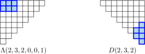
Refer to caption
Figure 14. Examples of the skew shape Λ(a,b,c,0,0,1)Λ𝑎𝑏𝑐001\Lambda(a,b,c,0,0,1) and the shifted shape D(a,b,c)𝐷𝑎𝑏𝑐D(a,b,c) that have equinumerous SYT.
Theorem 9.1 (Thm. V.3 [DeW]).

For the skew shape λ/μ=δa+b+2c/ba𝜆𝜇subscript𝛿𝑎𝑏2𝑐superscript𝑏𝑎\hskip 0.85355pt\lambda/\mu=\delta_{a+b+2c}/b^{a}, we have:

(9.2) sλ/μ=PD(a,b,c).subscript𝑠𝜆𝜇subscript𝑃𝐷𝑎𝑏𝑐s_{\lambda/\mu}\,=\,P_{D(a,b,c)}\hskip 1.70709pt.

By taking the coefficient of x1x2xnsubscript𝑥1subscript𝑥2subscript𝑥𝑛x_{1}x_{2}\ldots x_{n} in the equation above we obtain the following identity between the number of SYT of skew shape Λ(a,b,c,0,0,1)Λ𝑎𝑏𝑐001\Lambda(a,b,c,0,0,1) and shifted shape D(a,b,c)𝐷𝑎𝑏𝑐D(a,b,c).

Corollary 9.2 (Cor. V.7 [DeW]).

For the skew shape λ/μ=δa+b+2c/ba𝜆𝜇subscript𝛿𝑎𝑏2𝑐superscript𝑏𝑎\hskip 0.85355pt\lambda/\mu=\delta_{a+b+2c}/b^{a}, we have:

fλ/μ= 2|λ/μ|ab2c+1gD(a,b,c).superscript𝑓𝜆𝜇superscript2𝜆𝜇𝑎𝑏2𝑐1superscript𝑔𝐷𝑎𝑏𝑐f^{\lambda/\mu}\,=\,2^{|\lambda/\mu|-a-b-2c+1}g^{D(a,b,c)}\hskip 1.70709pt.

Combining this identity with the hook-length formula for gνsuperscript𝑔𝜈g^{\nu} (see e.g. [Sag2, Ex. 3.21]), we obtain a product formula for  fΛ(a,b,c,0,0,1)superscript𝑓Λ𝑎𝑏𝑐001f^{\Lambda(a,b,c,0,0,1)}  coinciding with that of Corollary 1.2. Similarly, by doing a stable principal specialization in (9.2) and using the Kawanaka product formula [Kaw] for this specialization of Schur P𝑃P-functions of straight shifted shapes, we obtain the formula in Corollary 4.4. This identity was obtained earlier and more generally by Krattenthaler and Schlosser, see Eq. (1.2) with n=a+b+2c𝑛𝑎𝑏2𝑐n=a+b+2c, m=b𝑚𝑏m=b and r=a𝑟𝑎r=a in [KS].

Note that DeWitt and Ardila–Serrano [AS] showed independently that the skew Schur function sδm/μsubscript𝑠subscript𝛿𝑚𝜇s_{\delta_{m}/\mu} has a positive expansion in the Schur P𝑃P-functions. From this expansion one can obtain Theorem 9.1.

It is natural to ask for a bijective proof of Corollary 9.2. Such a bijection combined with the hook-walk algorithm for shifted shapes [Sag1] or the bijective proof of the hook-length formula for gνsuperscript𝑔𝜈g^{\nu} [Fis], gives an algorithm to generate SYT of skew shape Λ(a,b,c,0,0,1)Λ𝑎𝑏𝑐001\Lambda(a,b,c,0,0,1) uniformly at random. We obtain the desired bijection in the followup work [M+].

9.5. Shifted shapes

One of the main results of this paper is to give families of skew shapes whose number of SYT is given by a product formula. A natural direction is to study the same question for shifted skew shapes.

Naruse in [Nar] also announced two formulas (of type B𝐵B and type D𝐷D) for the number of standard tableaux of shifted skew shape (see [MPP2, §§\S8]), in terms of analogues of excited diagrams.101010This result was recently proved and further generalized in [NO].

The type B𝐵B excited diagrams are obtained from the diagram of μ𝜇\mu by applying the following type B𝐵B excited moves:

[Uncaptioned image]

and     [Uncaptioned image]

We denote the set of type B𝐵B excited diagrams of shifted skew shape λ/μ𝜆𝜇\lambda/\mu by B(λ/μ)superscript𝐵𝜆𝜇\mathcal{E}^{B}(\lambda/\mu). Following the arguments in Section 2.7 and [MPP1, §3], the type B𝐵B excited diagrams of λ/μ𝜆𝜇\lambda/\mu are equivalent to certain flagged tableaux of shifted shape μ𝜇\mu and to certain non-intersecting paths (cf. [Ste]).

Question 9.3.

Is there a determinantal or Pfaffian formula for |B(λ/μ)|superscript𝐵𝜆𝜇|\mathcal{E}^{B}(\lambda/\mu)| counting the corresponding flagged tableaux of shifted shape μ𝜇\mu?

Given a shifted shape λ𝜆\lambda, the type B𝐵B hook of a cell (i,i)𝑖𝑖(i,i) in the diagonal is the set of cells in row i𝑖i of λ𝜆\lambda. The hook of a cell (i,j)𝑖𝑗(i,j) for ij𝑖𝑗i\leq j is the set of cells in row i𝑖i right of (i,j)𝑖𝑗(i,j), the cells in column j𝑗j below (i,j)𝑖𝑗(i,j), and if (j,j)𝑗𝑗(j,j) is one of these cells below then the hook also includes the cells in the j𝑗jth row of λ𝜆\lambda, thus counting (j,j)𝑗𝑗(j,j) twice overall. See Figure 15. The NHLF then extends verbatim for the number gλ/μsuperscript𝑔𝜆𝜇g^{\lambda/\mu} of standard tableaux of shifted skew shape λ/μ𝜆𝜇\lambda/\mu.

Theorem 9.4 (Naruse [Nar]).

Let λ,μ𝜆𝜇\lambda,\mu be partitions with distinct parts, such that μλ𝜇𝜆\mu\subset\lambda. We have

(9.3) gλ/μsuperscript𝑔𝜆𝜇\displaystyle g^{\lambda/\mu} =|λ/μ|!SB(λ/μ)(i,j)[λ]S1hB(i,j).absent𝜆𝜇subscript𝑆superscript𝐵𝜆𝜇subscriptproduct𝑖𝑗delimited-[]𝜆𝑆1superscript𝐵𝑖𝑗\displaystyle=|\lambda/\mu|!\sum_{S\in\mathcal{E}^{B}(\lambda/\mu)}\prod_{(i,j)\in[\lambda]\setminus S}\frac{1}{h^{B}(i,j)}\,.

Next we describe the shifted analogue of the thick reverse hook (Example 2.5).

Example 9.5 (shifted reverse hook).

For the shape Ra,c:=δa+c+1/δa+1assignsubscript𝑅𝑎𝑐subscript𝛿𝑎𝑐1subscript𝛿𝑎1R_{a,c}:=\delta_{a+c+1}/\delta_{a+1}, the type B𝐵B excited diagrams correspond to symmetric plane partitions with at most a+1𝑎1a+1 rows and largest part at most c𝑐c. By the Andrews–Gordon formula for symmetric plane partitions (see [Sta1]), we have:

|B(Ra,c)|=1ijak=1ci+j+k1i+j+k2=Φ(2a+c)Φ(a)Φ(2a)Φ(a+c)(2a)(c)(2a+c).superscript𝐵subscript𝑅𝑎𝑐subscriptproduct1𝑖𝑗𝑎superscriptsubscriptproduct𝑘1𝑐𝑖𝑗𝑘1𝑖𝑗𝑘2Φ2𝑎𝑐Φ𝑎Φ2𝑎Φ𝑎𝑐2𝑎𝑐2𝑎𝑐|\mathcal{E}^{B}(R_{a,c})|\,=\,\prod_{1\leq i\leq j\leq a}\hskip 1.70709pt\prod_{k=1}^{c}\,\frac{i+j+k-1}{i+j+k-2}\,=\,\hskip 1.70709pt\frac{\Phi(2a+c)\hskip 1.70709pt\Phi(a)}{\Phi(2a)\hskip 1.70709pt\Phi(a+c)}\,\cdot\,\frac{\gimel(2a)\hskip 1.70709pt\gimel(c)}{\gimel(2a+c)}\,.

It is natural to study shifted analogues of our product formulas for skew shapes. For nonnegative integers ac,d𝑎𝑐𝑑a\leq c,d and m𝑚m, let λ/μ=Λ(a,c,d,m)𝜆𝜇superscriptΛ𝑎𝑐𝑑𝑚\lambda/\mu=\Lambda^{\triangledown}(a,c,d,m) be the following shifted skew partition

λ=(c+a,c+a1,,1)+ν,𝜆𝑐𝑎𝑐𝑎11𝜈\lambda\hskip 1.70709pt=\hskip 1.70709pt(c+a,c+a-1,\ldots,1)\hskip 1.70709pt+\hskip 1.70709pt\nu\hskip 0.85355pt,

where ν=(d+(a+c1)m,d+(a+c2)m,,d)𝜈𝑑𝑎𝑐1𝑚𝑑𝑎𝑐2𝑚𝑑\hskip 0.85355pt\nu=(d+(a+c-1)m,d+(a+c-2)m,\ldots,d)  and μ=δa+1𝜇subscript𝛿𝑎1\hskip 0.85355pt\mu=\delta_{a+1}. See Figure 15.

Refer to caption
Figure 15. Left: example of the type B𝐵B hook of a cell (i,j)𝑖𝑗(i,j) of λ𝜆\lambda of length 999 (cell (3,3)33(3,3) is counted twice), and the type B𝐵B hook-lengths of the cells of the shifted shape (5,3,1)531(5,3,1). Right: The shifted skew shape Λ(a,c,d,m)superscriptΛ𝑎𝑐𝑑𝑚\Lambda^{\triangledown}(a,c,d,m) and the shape whose hooks appear in the product formula in Conjecture 9.6.

Computations using the Pfaffian formula for gλ/μsuperscript𝑔𝜆𝜇g^{\lambda/\mu} (see [Iva, Thm. 7.5]), suggest the following conjectured111111This conjecture was recently established in [KY]. product formula for these shifted skew shapes.

Conjecture 9.6.

In the notation above, for  π=Λ(a,c,d,m)𝜋superscriptΛ𝑎𝑐𝑑𝑚\pi=\Lambda^{\triangledown}(a,c,d,m), we have:

gπ=n!2aΦ(2a+c)Φ(a)Φ(2a)Φ(a+c)(2a)(c)(2a+c)uλ(δa+c+1/caδc+1)1hB(u).superscript𝑔𝜋𝑛superscript2𝑎Φ2𝑎𝑐Φ𝑎Φ2𝑎Φ𝑎𝑐2𝑎𝑐2𝑎𝑐subscriptproduct𝑢𝜆subscript𝛿𝑎𝑐1superscript𝑐𝑎subscript𝛿𝑐11subscript𝐵𝑢g^{\pi}\,=\,\frac{n!}{2^{a}}\,\cdot\,\frac{\Phi(2a+c)\hskip 1.70709pt\Phi(a)}{\Phi(2a)\hskip 1.70709pt\Phi(a+c)}\,\cdot\,\frac{\gimel(2a)\hskip 1.70709pt\gimel(c)}{\gimel(2a+c)}\,\cdot\,\prod_{u\in\lambda\setminus(\delta_{a+c+1}/c^{a}\delta_{c+1})}\,\frac{1}{h_{B}(u)}\,.

See Figure 15 for an illustration of the cells of the shifted shape λ𝜆\lambda whose hook-lengths appear in the conjectured formula above. The special case  π=Λ(a,c,d,0)𝜋superscriptΛ𝑎𝑐𝑑0\pi=\Lambda^{\triangledown}(a,c,d,0)  is the (conjugated) truncated rectangle shape, and was established by the third author using a different technique [Pan] and later in [KO1, Cor. 4.6] by yet again different methods. In particular, for  π=Λ(a,c,0,0)𝜋superscriptΛ𝑎𝑐00\pi=\Lambda^{\triangledown}(a,c,0,0), we obtain the product formula for shifted reverse hook in the example above. This both lends support to the conjecture and explains its appearance, which seemed out of place until now, see [AdR].

9.6. Racah and q𝑞q-Racah formulas

In the Appendix of [BGR], the authors generalize the MacMahon box formula (2.1) to five variables, which they formulate in terms of lozenge tilings of H(a,b,c)H𝑎𝑏𝑐\operatorname{H}(a,b,c) with weights F(p,q,u1,u2,u3)𝐹𝑝𝑞subscript𝑢1subscript𝑢2subscript𝑢3F(p,q,u_{1},u_{2},u_{3}) given by products of certain elliptic functions (see Theorem 10.5 in [BGR]). Upon seeing our main technical tool, Theorem 3.10, Eric Rains noticed121212Personal communication. that there is a common special case of both formulas giving the q𝑞q-Racah formula. In the notation of [BGR], let u1=usubscript𝑢1𝑢u_{1}=u, u2=u3=0subscript𝑢2subscript𝑢30u_{2}=u_{3}=0, p0𝑝0p\to 0  to get the following result:

Corollary 9.7 (Appendix to [BGR]).

We have:

(9.4) Π[a×b×c](i,j,k)Πqqj+k2iu1qj+k2i+1u=(i,j,k)[a×b×c](1qi+j+k1)(1qj+ki1u)(1qi+j+k2)(1qj+kiu),subscriptΠdelimited-[]𝑎𝑏𝑐subscriptproduct𝑖𝑗𝑘Π𝑞superscript𝑞𝑗𝑘2𝑖𝑢1superscript𝑞𝑗𝑘2𝑖1𝑢subscriptproduct𝑖𝑗𝑘delimited-[]𝑎𝑏𝑐1superscript𝑞𝑖𝑗𝑘11superscript𝑞𝑗𝑘𝑖1𝑢1superscript𝑞𝑖𝑗𝑘21superscript𝑞𝑗𝑘𝑖𝑢\sum_{\Pi\hskip 1.70709pt\subset\hskip 1.70709pt[a\times b\times c]}\,\prod_{(i,j,k)\hskip 0.85355pt\in\hskip 0.85355pt\Pi}\,\frac{q-q^{j+k-2i}u}{1-q^{j+k-2i+1}u}\ \,=\,\prod_{(i,j,k)\hskip 0.85355pt\in\hskip 1.70709pt[a\times b\times c]}\frac{(1-q^{i+j+k-1})(1-q^{j+k-i-1}u)}{(1-q^{i+j+k-2})(1-q^{j+k-i}u)}\,,

where the summation is over all plane partitions ΠΠ\Pi which fit inside the box  [a×b×c]delimited-[]𝑎𝑏𝑐[a\times b\times c].

In the notation of Theorem 3.10, this identity follows by considering the hexagon  H(b,c,a)H𝑏𝑐𝑎\operatorname{H}(b,c,a) (a𝑎a is the height this time), so μ=bc𝜇superscript𝑏𝑐\mu=b^{c}, then setting  xi=qi+asubscript𝑥𝑖superscript𝑞𝑖𝑎x_{i}=q^{-i+a}, yj=uqja1subscript𝑦𝑗𝑢superscript𝑞𝑗𝑎1y_{j}=uq^{j-a-1}, and noting that the RHS factors. We omit the details.

For u=0𝑢0u=0, equation (9.4) gives the MacMahon q𝑞q-formula (2.2), where the sum is over plane partitions, while the Racah formula follows by letting q,u=qh1𝑞𝑢superscript𝑞1q,\hskip 0.85355ptu=q^{h}\hskip 0.85355pt\to 1

(9.5) Π[a×b×c](i,j,k)Πj+k2i1+hj+k2i+1+h=(i,j,k)[a×b×c](i+j+k1)(j+ki1+h)(i+j+k2)(j+ki+h).subscriptΠdelimited-[]𝑎𝑏𝑐subscriptproduct𝑖𝑗𝑘Π𝑗𝑘2𝑖1𝑗𝑘2𝑖1subscriptproduct𝑖𝑗𝑘delimited-[]𝑎𝑏𝑐𝑖𝑗𝑘1𝑗𝑘𝑖1𝑖𝑗𝑘2𝑗𝑘𝑖\sum_{\Pi\hskip 1.70709pt\subset\hskip 1.70709pt[a\times b\times c]}\,\prod_{(i,j,k)\hskip 0.85355pt\in\hskip 0.85355pt\Pi}\,\frac{j+k-2i-1+h}{j+k-2i+1+h}\,\ =\,\prod_{(i,j,k)\hskip 0.85355pt\in\hskip 1.70709pt[a\times b\times c]}\,\frac{(i+j+k-1)(j+k-i-1+h)}{(i+j+k-2)(j+k-i+h)}\,.

When a=1𝑎1a=1, this gives (3.8), since plane partitions of height 1 correspond to a single lattice path. Finally, when hh\to\infty, this identity gives the MacMahon box formula (2.1).

9.7. Excited diagrams and Grothendieck polynomials

In addition to Theorem 5.1, Knutson–Miller–Yong [KMY, Thm. 5.8] also gave a formula for the Grothendieck polynomials of vexillary permutations in terms of a larger class of diagrams called generalized excited diagrams. For the shape λ/μ𝜆𝜇\lambda/\mu these diagrams are defined as follows: for each active cell (i,j)𝑖𝑗(i,j) we do two types of generalized excited moves:  (i) the usual move replacing (i,j)𝑖𝑗(i,j) by (i+1,j+1)𝑖1𝑗1(i+1,j+1), or (ii) the move which keeps (i,j)𝑖𝑗(i,j) and adds (i+1,j+1)𝑖1𝑗1(i+1,j+1) :

[Uncaptioned image]

or      [Uncaptioned image]

These diagrams were also studied by Kreiman [Kre] and they are in correspondence with set valued flagged tableaux. In [MPP6], we use these diagrams to give a generalization of Naruse’s formula (NHLF) and the analysis in Section 5 for Grothendieck polynomials.
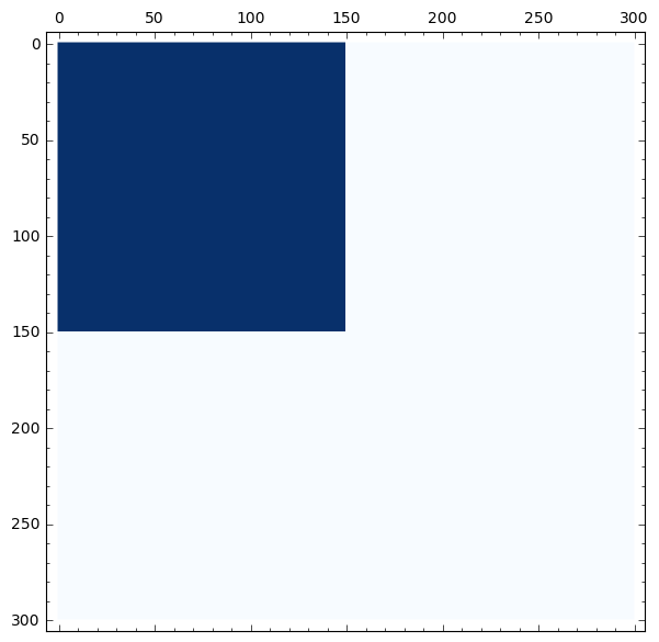
Refer to caption
Refer to caption
Refer to caption
Figure 16. A random excited diagram of shape 300300/150150superscript300300superscript150150300^{300}/150^{150} (left), in the uniform (middle), and the hook-weighted distribution (right).

9.8. Limit shapes

Since excited diagrams are in bijection with lozenge tilings (see Theorem 7.2), one can translate known limit shape results for tilings into the language of excited diagrams. For example, the middle picture in Figure 16 is a random excited diagram of shape  300300/150150superscript300300superscript150150300^{300}/150^{150}. These are obtained by running a Metropolis algorithm for  1010superscript101010^{10}  steps. The visible limit shape is in fact a stretched circle.

Similarly, since SYT(λ/μ)SYT𝜆𝜇\operatorname{{\rm SYT}}(\lambda/\mu) are enumerated by the weighted excited diagrams (by a product of hooks of the squares in the diagram), one can ask about limit shapes of hook weighted lozenge tilings. An example of a clearly visible limit shape is shown in the right picture in Figure 16. Both examples are a larger version of the lozenge tilings in Figure 2.
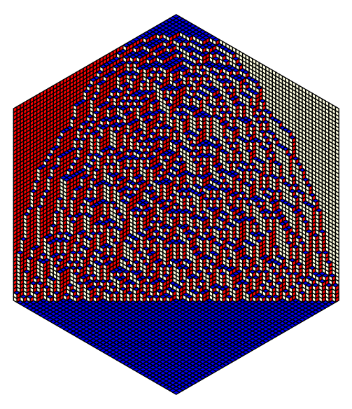
Refer to caption
Refer to caption
Figure 17. Uniform and hook-weighted lozenge tilings of the hexagon H(50,50,50)H505050\operatorname{H}(50,50,50) slanted by a diagonal.

Note that sometimes it is easier to analyze the limit shape for the lozenge tilings than for the other skew shapes like staircases. For examples, in Figure 17 we show two lozenge tilings of the hexagon H(50,50,50)H505050\operatorname{H}(50,50,50) slanted by a diagonal, one corresponding to the uniform excited diagram of the staircase π=δ150/δ50𝜋subscript𝛿150subscript𝛿50\pi=\delta_{150}/\delta_{50}, and another with the hook weights. These random tilings are obtained by running a Metropolis algorithm for  31093superscript1093\cdot 10^{9}  steps. While the limit shapes have roughly similar outlines, in the uniform case the limit shape curves are visibly tangent to the vertical sides of the hexagon, and in the hook weighted case form an acute angle.

The observed behavior in the uniform case here is in line with the cases of lozenge tilings of polygonal regions; for such regions the frozen boundary is an inscribed algebraic curve as shown in e.g. [KO, KOS]. However, the hexagon with slanted diagonal is not a region which has been treated with any of the classical methods even in the uniform case. It would be interesting to obtain the exact form of the limit shape in the hook weighted case in connection with our detailed study of fπsuperscript𝑓𝜋f^{\pi} in [MPP3, MPP5]; see [Rom] for some related results.


Acknowledgements

We are grateful to Sami Assaf, Dan Betea, Sara Billey, Valentin Féray, Vadim Gorin, Zach Hamaker, Tri Lai, Leonid Petrov, Dan Romik, Luis Serrano, Richard Stanley, Hugh Thomas, Nathan Williams, Damir Yeliussizov and Alex Yong for useful comments and help with the references, and to Jane Austen [Aus] for the inspiration behind the first sentence. We are very thankful to Eric Rains for showing us the connections to Racah polynomials (see §§\S9.6), to Christian Krattenthaler for pointing out to us the paper [KS] and graciously allowing us to publish his conjectural formula (5.8), and to Jang Soo Kim for pointing us out that Corollary 1.1 appeared in [KO1]. We thank the anonymous referees for their careful reading, comments, and suggestions. The lozenge tilings in figures 2 and 17 were made using Sage and its algebraic combinatorics features developed by the Sage-Combinat community [Sage]. Martin Tassy generously helped us with the Metropolis simulations. The first author was partially supported by an AMS-Simons travel grant. The second and third authors were partially supported by the NSF.


References

  • [AdR] R. Adin and Y. Roichman, Standard Young tableaux, in Handbook of Enumerative Combinatorics (M. Bóna, editor), CRC Press, Boca Raton, 2015, 895–974.
  • [AsR] R. A. Askey and R. Roy, Barnes G𝐺G-function, in F. W. J. Olver et al., NIST Handbook of Mathematical Functions, Cambridge Univ. Press, 2012.
  • [AS] F. Ardila and L. G. Serrano, Staircase skew Schur functions are Schur P-positive, J. Algebraic Combin. 36 (2012), 409–423.
  • [Aus] J. Austen, Pride and Prejudice, vol. I–III, T. Egerton, London, England, 1813.
  • [Bet] D. Betea, Elliptic Combinatorics and Markov Processes, Ph.D. thesis, Caltech, 2012, 124 pp.
  • [BR] Y. Baryshnikov and D. Romik, Enumeration formulas for Young tableaux in a diagonal strip, Israel J. Math. 178 (2010), 157–186.
  • [BHY] S. Billey, A. E. Holroyd and B. Young, A bijective proof of Macdonald’s reduced word formula, to appear in Algebraic Combinatorics; arXiv:1702.02936.
  • [BJS] S. C. Billey, W. Jockusch and R. P. Stanley, Some Combinatorial Properties of Schubert Polynomials, J. Algebraic Combin. 2 (1993), 345–374.
  • [BG] A. Borodin and V. Gorin, Shuffling algorithm for boxed plane partitions, Adv. Math. 220 (2009), 1739–1770.
  • [BGR] A. Borodin, V. Gorin and E. M. Rains, q𝑞q-distributions on boxed plane partitions, Selecta Math. 16 (2010), 731–789.
  • [Bre] D. M. Bressoud, Proofs and confirmations. The story of the alternating sign matrix conjecture, Cambridge Univ. Press, Cambridge, 1999.
  • [CLP] H. Cohn, M. Larsen and J. Propp, The Shape of a Typical Boxed Plane Partition, New York J. Math. 4 (1998), 137–165.
  • [DeW] E. A. DeWitt, Identities Relating Schur s𝑠s-Functions and Q𝑄Q-Functions, Ph.D. thesis, University of Michigan, 2012, 73 pp.; available at  https://tinyurl.com/y9ktq5v7.
  • [DF] J. Dousse and V. Féray, Asymptotics for skew standard Young tableaux via bounds for characters; arXiv:1710.05652.
  • [Fis] I. Fischer, A bijective proof of the hook-length formula for shifted standard tableaux, arXiv:math/ 0112261.
  • [FS] P. Flajolet and R. Sedgewick, Analytic combinatorics, Cambridge Univ. Press, Cambridge, 2009.
  • [FK] S. Fomin and A. N. Kirillov, Reduced words and plane partitions, J. Algebraic Combin. 6 (1997), 311–319.
  • [GP] V. Gorin and G. Panova, Asymptotics of symmetric polynomials with applications to statistical mechanics and representation theory, Ann. Probab. 43 (2015), 3052–3132.
  • [Gow] W. T. Gowers, The two cultures of mathematics, in Mathematics: frontiers and perspectives, AMS, Providence, RI, 2000, 65–78.
  • [GNW] C. Greene, A. Nijenhuis and H. S. Wilf, A probabilistic proof of a formula for the number of Young tableaux of a given shape, Adv. Math. 31 (1979), 104–109.
  • [IN] T. Ikeda and H. Naruse, Excited Young diagrams and equivariant Schubert calculus, Trans. AMS 361 (2009), 5193–5221.
  • [Iva] V. N. Ivanov, Interpolation Analogs of Schur Q-Functions, J. Math. Sci. 131 (2005), 5495–5507
  • [Kaw] N. Kawanaka, A q𝑞q-series identity involving Schur functions and related topics, Osaka J. Math. 36 (1999), 157–176.
  • [Ken1] R. Kenyon, Height fluctuations in the honeycomb dimer model, Comm. Math. Phys. 281 (2008), 675–709.
  • [Ken2] R. Kenyon, Lectures on dimers, in Statistical Mechanics, AMS, 2009.
  • [KO] R. Kenyon and A. Okounkov, Limit shapes and Burgers equation, Acta Math. 199 (2007), 263–302.
  • [KOS] R. Kenyon, A. Okounkov and S. Sheffield, Dimers and amoebae, Annals of Math. 163 (2006), 1019–1056.
  • [KO1] J. S. Kim and S. Oh, The Selberg integral and Young books, J. Combin. Theory Ser. A 145 (2017), 1–24.
  • [KOk] J. S. Kim and S. Okada, A new q𝑞q-Selberg integral, Schur functions, and Young books, Ramanujan J. 42 (2017), 43–57.
  • [KY] J. S. Kim and M.  Yoo, Product formulas for certain skew tableaux; arXiv:1806.01525.
  • [Kit] S. Kitaev, Patterns in permutations and words, Springer, Heidelberg, 2011.
  • [KMY] A. Knutson, E. Miller and A. Yong, Gröbner geometry of vertex decompositions and of flagged tableaux, J. Reine Angew. Math. 630 (2009), 1–31.
  • [KT] A. Knutson and T. Tao, Puzzles and (equivariant) cohomology of Grassmannians, Duke Math J. 119 (2003), 221–260.
  • [Kra1] C. Kratthenthaler, Generating functions for plane partitions of a given shape, Manuscripta Math. 69 (1990), 173–201.
  • [Kra2] C. Kratthenthaler, Advanced determinant calculus, Sém. Lothar. Combin. 42 (1999), Art. B42q, 67 pp.
  • [Kra3] C. Kratthenthaler, Advanced determinant calculus: a complement, Linear Algebra Appl. 411 (2005), 68–166.
  • [KS] C. Kratthenthaler and M. Schlosser, The major index generating function of standard Young tableaux of shapes of the form “staircase minus rectangle”, Contemp. Math. 627 (2014), 111–122.
  • [Kre] V. Kreiman, Schubert classes in the equivariant K-theory and equivariant cohomology of the Grassmannian; arXiv:math.AG/0512204.
  • [Kup1] G. Kuperberg, Another proof of the alternating-sign matrix conjecture, IMRN 1996, no. 3, 139–150.
  • [Kup2] G. Kuperberg, Symmetry classes of alternating-sign matrices under one roof, Annals of Math. 156 (2002), 835–866.
  • [Lai1] T. Lai, Enumeration of tilings of quasi-hexagons, hexagonal dungeons, quartered hexagons, and variants of the Aztec diamond, Ph.D. thesis, Indiana University, 2014, 217 pp.
  • [Lai2] T. Lai, A q𝑞q-enumeration of lozenge tilings of a hexagon with three dents, Adv. Appl. Math. 82 (2017), 23–57.
  • [LRS] V. Lakshmibai, K. N. Raghavan and P. Sankaran, Equivariant Giambelli and determinantal restriction formulas for the Grassmannian; arXiv:math/0506015.
  • [Las] A. Lascoux, Polynomials, monograph draft, 2013; https://tinyurl.com/y8z2dlna
  • [LS1] A. Lascoux and M.-P. Schützenberger, Polynômes de Schubert (in French), C. R. Acad. Sci. Paris Sér I, Math. 294 (1982), 447–450.
  • [LS2] A. Lascoux and M.-P. Schützenberger, Structure de Hopf de l’anneau de cohomologie et de l’anneau de Grothendieck d’une variété de drapeaux (in French), C. R. Acad. Sci. Paris Sér. I Math. 295 (1982), 629–633.
  • [Mac] I. G. Macdonald, Notes on Schubert polynomials, Publ. LaCIM, UQAM, 1991.
  • [Man] L. Manivel, Symmetric functions, Schubert polynomials and degeneracy loci, SMF/AMS, 2001.
  • [MeS] G. Merzon and E. Smirnov, Determinantal identities for flagged Schur and Schubert polynomials, Eur. J. Math. 2 (2016), 227–245.
  • [MoS] A. I. Molev and B. E. Sagan, A Littlewood–Richardson rule for factorial Schur functions, Trans. AMS 351 (1999), 4429–4443.
  • [M+] A. H. Morales, Z. Hamaker, I. Pak, L. Serrano and N. Williams, in preparation.
  • [MPP1] A. H. Morales, I. Pak and G. Panova, Hook formulas for skew shapes I. q𝑞q-analogues and bijections, J. Combin. Theory, Ser. A 154 (2018), 350–405.
  • [MPP2] A. H. Morales, I. Pak and G. Panova, Hook formulas for skew shapes II. Combinatorial proofs and enumerative applications, SIAM J. Discrete Math. 31 (2017), 1953–1989.
  • [MPP3] A. H. Morales, I. Pak and G. Panova, Asymptotics for the number of standard Young tableaux of skew shape, European J. Combin. 70 (2018), 26–49.
  • [MPP4] A. H. Morales, I. Pak and G. Panova, Asymptotics of principal evaluations of Schubert polynomials for layered permutations, to appear in Proc. AMS; arXiv:1805.04341.
  • [MPP5] A. H. Morales, I. Pak and G. Panova, Asymptotics of the number of standard Young tableaux of skew shape II. The case of thick ribbons, in preparation.
  • [MPP6] A. H. Morales, I. Pak and G. Panova, Hook formulas for skew shapes IV. Increasing tableaux and factorial Grothendieck polynomials, in preparation.
  • [MPT] A. H. Morales, I. Pak and M. Tassy, Asymptotics for the number of standard tableaux of skew shape and for weighted lozenge tilings; arXiv:1805.00992.
  • [Nar] H. Naruse, Schubert calculus and hook formula, talk slides at 73rd Sém. Lothar. Combin., Strobl, Austria, 2014; available at  tinyurl.com/z6paqzu.
  • [NO] H. Naruse and S. Okada, Skew hook formula for d𝑑d-complete posets; arXiv:1802.09748.
  • [NPS] J.-C. Novelli, I. Pak and A. V. Stoyanovskii, A direct bijective proof of the hook-length formula, Discrete Math. Theor. Comput. Sci. 1 (1997), 53–67.
  • [Pak] I. Pak, Tile invariants: new horizons, Theor. Comp. Sci. 303 (2003), 303–331.
  • [Pan] G. Panova, Tableaux and plane partitions of truncated shapes, Adv. Appl. Math. 49 (2012), 196–217.
  • [Pet] L. Petrov, Asymptotics of random lozenge tilings via Gelfand–Tsetlin schemes, Prob. Theory Rel. Fields 160 (2015), 429–487
  • [Pro] R. A. Proctor, New symmetric plane partition identities from invariant theory work of De Concini and Procesi, Europ. J. Combin. 11 (1990), 289–300.
  • [Rom] D. Romik, Arctic circles, domino tilings and square Young tableaux, Ann. Probab. 40 (2012), 611–647.
  • [Rota] G.-C. Rota, Ten lessons I wish I had been taught, Notices AMS 44 (1997), 22–25.
  • [Sag1] B. E. Sagan, On selecting a random shifted Young tableau, J. Algorithms 1 (1980), 213–234.
  • [Sag2] B. E. Sagan, The Symmetric Group, Springer, 2000.
  • [Sage] The Sage-Combinat community. Sage-Combinat: enhancing Sage as a toolbox for computer exploration in algebraic combinatorics, 2017. http://combinat.sagemath.org.
  • [SeS] L. Serrano and C. Stump, Maximal Fillings of Moon Polyominoes, Simplicial Complexes, and Schubert Polynomials, Electron. J. Combin. 19:1 (2012), P16, 18 pp.
  • [OEIS] N. J. A. Sloane, The Online Encyclopedia of Integer Sequences, oeis.org.
  • [Sta1] R. P. Stanley, Plane Partitions: Past, Present, and Future, Ann. N.Y. Acad. Sci. 555 (1989), 397--401.
  • [Sta2] R. P. Stanley, Enumerative Combinatorics, vol. 1 and 2, Cambridge Univ. Press, 2012 and 1999.
  • [Sta3] R. P. Stanley, A survey of alternating permutations, in Combinatorics and graphs, AMS, Providence, RI, 2010, 165--196.
  • [Sta4] R. P. Stanley, Some Schubert shenanigans, arXiv:1704.00851.
  • [Ste] J. R. Stembridge, Nonintersecting paths, pfaffians, and plane partitions, Adv. Math. 83 (1990), 96--131.
  • [Thu] W. P. Thurston, Groups, tilings and finite state automata, in Lecture Notes, AMS Summer Meetings, Bolder, CO, 1989.
  • [Wac] M. Wachs, Flagged Schur functions, Schubert polynomials, and symmetrizing operators, J. Combin. Theory, Ser. A 40 (1985), 276--289.
  • [Wei] A. Weigandt, Schubert polynomials, 132-patterns, and Stanley’s conjecture, to appear in Algebraic Combinatorics; arXiv:1705.02065.
  • [Woo] A. Woo, Catalan numbers and Schubert polynomials for w=1(n+1)2𝑤1𝑛12w=1(n+1)\ldots 2, arXiv:math/0407160.