Aging Feynman-Kac Equation

Wanli Wang    Weihua Deng dengwh@lzu.edu.cn 1School of Mathematics and Statistics, Gansu Key Laboratory of Applied Mathematics and Complex Systems, Lanzhou University, Lanzhou 730000, P.R. China
Abstract

Aging, the process of growing old or maturing, is one of the most widely seen natural phenomena in the world. For the stochastic processes, sometimes the influence of aging can not be ignored. For example, in this paper, by analyzing the functional distribution of the trajectories of aging particles performing anomalous diffusion, we reveal that for the fraction of the occupation time T+/tsubscript𝑇𝑡T_{+}/t of strong aging particles, (T+(t)2)=12t2delimited-⟨⟩superscript𝑇superscript𝑡212superscript𝑡2\langle(T^{+}(t)^{2})\rangle=\frac{1}{2}t^{2} with coefficient 1212\frac{1}{2}, having no relation with the aging time tasubscript𝑡𝑎t_{a} and α𝛼\alpha and being completely different from the case of weak (none) aging. In fact, we first build the models governing the corresponding functional distributions, i.e., the aging forward and backward Feynman-Kac equations; the above result is one of the applications of the models. Another application of the models is to solve the asymptotic behaviors of the distribution of the first passage time, g(ta,t)𝑔subscript𝑡𝑎𝑡g(t_{a},t). The striking discovery is that for weakly aging systems, g(ta,t)taα2t1α2similar-to𝑔subscript𝑡𝑎𝑡superscriptsubscript𝑡𝑎𝛼2superscript𝑡1𝛼2g(t_{a},t)\sim t_{a}^{\frac{\alpha}{2}}t^{-1-\frac{\alpha}{2}}, while for strongly aging systems, g(ta,t)𝑔subscript𝑡𝑎𝑡g(t_{a},t) behaves as taα1tαsuperscriptsubscript𝑡𝑎𝛼1superscript𝑡𝛼t_{a}^{\alpha-1}t^{-\alpha}.

Aging, Renewal Process, Feynman-Kac Equation
pacs:
02. 50. -r, 05. 30. Pr, 05. 40. -a, 05. 10. Gg

I Introduction

One of the most omnipresent phenomena in nature is aging, being clearly a process of time t𝑡t. The models naturally coming into our mind are the stochastic processes, the leading examples of which are the renewal processes. As the generalization of Poisson process Papoulis:84 , in this paper, we mainly focus on the renewal processes with independent identically distributed (i.i.d.) holding times between any adjacent two renews, and the distribution of holding times is power law with divergent first moment. Not like Poisson process, in this case, the power law renewal process is not longer Markovian, which leads to nonstationarity, exhibiting aging behaviors Barkai2002Aging .

For the power law renewal process, if there is a jump for each renewal, we get the compound power law renewal process; the size of jump is generally an i.i.d. random variable with specified probability distribution. This compound renew process can effectively characterize anomalous diffusion Krusemann:01 , whose mean squared displacement is a nonlinear function of time t𝑡t, i.e.,

x2(t)Kαtα;similar-to-or-equalsdelimited-⟨⟩superscript𝑥2𝑡subscript𝐾𝛼superscript𝑡𝛼\left<x^{2}(t)\right>\simeq K_{\alpha}t^{\alpha}; (1)

if the second moment of the variable of the size of the jump is bounded, the process describes subdiffusion, which means α(0,1)𝛼01\alpha\in(0,1); on the other side, if the second moment diverges, the process is for the competition between long rests and long jumps Metzler:00 , and the resulted macroscopic behavior may be superdiffusion, subdiffusion, or even normal diffusion.

Anomalous diffusion phenomena are ubiquitous in real life. For example, they are found in systems including ultra-cold atoms, telomeres in the nucleus of cells Bronstein2009Transient , bacterial motion Nossal1983Stochastic , and even the flight of an albatross Viswanathan1996levy . Anomalous diffusion in the presence or absence of force fields has been modelled in many ways such as generalised diffusion equations OShaughnessy1985Analytical , fractional Brownian motion Mandelbrot1968Fractional , continue time random walk Klafter2011First ; Metzler20001The (CTRW), Langenvin equations Bruce1982Linear ; Fogedby1994Levy , and so on. The compound power law renewal process is a specific class of CTRW model, where both waiting time and jump length are i.i.d. random variables, in particular, the distribution of waiting time is power law with divergent first moment. Generally, for the CTRW model, the physical clock is assumed to start at the first step of the process, i.e., we have to observe or measure the system immediately after its preparation in the present state. For the real physical process, the observation time should not be exactly the starting time of the process. Monthus and Bouchaud Monthus1996Models introduce a CTRW framework, which can be used to study aging behaviors. It is called generalized CTRW or aging continuous time random walk (ACTRW) Barkai2002Aging , where the measure time starts not at time t=0𝑡0t=0 but at some later instant time t=ta>0𝑡subscript𝑡𝑎0t=t_{a}>0 and tasubscript𝑡𝑎t_{a} denotes the aging time.

There are already some research works for the aging in complex systems Barkai2003Aging ; Klafter2011First ; Marinari1993On ; Doussal1999Random ; Sokolov2001Linear ; and the aging behaviors are observed in the fluorescence of single nanocrystals Brokmann2003Statistic , polymers Struick1978Physical , time average of single particle trajectories in scale-free anomalous diffusion processes Schulz2013Aging . Here we further discuss the aging behavior in complex system by analyzing the functional distribution of the trajectories of the aging particles. The functional A𝐴A is defined as

A=0tU(x(τ))𝑑τ,𝐴superscriptsubscript0𝑡𝑈𝑥𝜏differential-d𝜏A=\int_{0}^{t}U(x(\tau))d\tau, (2)

where U𝑈U is a prescribed function and x(t)𝑥𝑡x(t) is the trajectory of the particle. Based on Eq. (2), many interesting applications have been dug out. If one is concerned about the time spent by a particle in a given domain, it can be made by taking U=1𝑈1U=1 if the particle lies in the domain and 00 otherwise Luchinin2014Application ; Bar-Haim1998On ; Wu2016Tempered . The functional is also used to study NMR Grebenkov2007NMR ; under the influence of inhomogeneous magnetic U(x(t))𝑈𝑥𝑡U(x(t)), the total phase accumulated along the trajectory of a nucleus during the time from 00 to t𝑡t is taken as

ϑ(t)=γ0tU(x(τ))𝑑τ,italic-ϑ𝑡𝛾superscriptsubscript0𝑡𝑈𝑥𝜏differential-d𝜏\vartheta(t)=\gamma\int_{0}^{t}U(x(\tau))d\tau,

where γ𝛾\gamma is the nuclear gyromagnetic ratio; and U(x)𝑈𝑥U(x) is respectively specified as x𝑥x and x2superscript𝑥2x^{2} to calculate the macroscopic measured signal E=exp(iϑ(t))𝐸delimited-⟨⟩𝑖italic-ϑ𝑡E=\langle\exp(i\vartheta(t))\rangle; then, NMR indirectly encodes information regarding the trajectory of the particles. If U=δ(xa)𝑈𝛿𝑥𝑎U=\delta(x-a), the functional A𝐴A denotes the local time at the fixed level a𝑎a, which is an important quality in probability Pitman1999The . Yet another instance used in finance is the case U(x)=exp(x)𝑈𝑥𝑥U(x)=\exp(x), which illustrates the price of an Asian stock option in the Black-Scholes framework Fischer1973The . Interestingly, these functionals A𝐴A and their related variants are also used as a powerful tool in mathematics and physics, i.e., Feynman-Kac formula, which allows to study the functionals in a quantum mechanical framework Majumdar2005Brownian ; Kac1949On ; Perret2015On ; Baule2006Investigation ; Majumdar2002Large ; Carmi2010On .

This paper is organized as follows. In Sect. II, based on the ACTRW model, we derive the forward Feynman-Kac equation with (tempered) power law waiting time. We start from the simple case, i.e., the probability density function (PDF) of the step length is taken as f(x)=12[δ(xa)+δ(x+a)]𝑓𝑥12delimited-[]𝛿𝑥𝑎𝛿𝑥𝑎f(x)=\frac{1}{2}[\delta(x-a)+\delta(x+a)], which implies that the particles can only move to the left or right direction with the same probability; then we use Gaussian distribution and power law distribution, respectively, as the PDF of jump length. If letting p=0𝑝0p=0, one obtains a generalization of the Montroll-Weiss equation for ACTRW, which agrees with the previous result Barkai2003Aging ; Klafter2011First . In Sect. III, we obtain the corresponding backward Feynman-Kac equations. Based on the derived equations, some applications are presented, such as the occupation in half space T+superscript𝑇T^{+}, the moments of T+superscript𝑇T^{+} and (T+)2superscriptsuperscript𝑇2(T^{+})^{2}. The behaviors of (T+)2delimited-⟨⟩superscriptsuperscript𝑇2\langle(T^{+})^{2}\rangle are different for strong and weak (none) aging. Furthermore, the asymptotic behaviors of the first passage time are analyzed for both the cases of strong and weak aging. In the last section, we conclude the paper with some discussions.

II Derivation of the fractional forward aging Feynman-Kac Equation

Based on ACTRW, we derive its corresponding forward Feynman-Kac equations, including the cases that the particles move with constant jump length, and the power law jump length and (tempered) power law waiting times. Now, we first briefly outline the main ingredients of the CTRW Montroll1965Random ; Kenkre1973Generalized ; Gorenflo2007Continue and ACTRW Barkai2003Aging ; Klafter2011First ; Marinari1993On ; Brokmann2003Statistic ; Struick1978Physical . CTRW and ACTRW are defined as follows: a walker is trapped on the origin for the time t1subscript𝑡1t_{1}, then makes a jump and the displacement is x1subscript𝑥1x_{1}; the walker is further trapped on x1subscript𝑥1x_{1} for time t2subscript𝑡2t_{2}, and then jumps to a new position; this process is then renewed. Both of them are characterized by a set of waiting times {t1,t2,,tn,}subscript𝑡1subscript𝑡2subscript𝑡𝑛\{t_{1},t_{2},\cdots,t_{n},\cdots\} and the displacements {x1,x2,,xn,}subscript𝑥1subscript𝑥2subscript𝑥𝑛\{x_{1},x_{2},\cdots,x_{n},\cdots\}. For both CTRW and ACTRW, all xisubscript𝑥𝑖x_{i} are i.i.d. with a common PDF f(x)|x|1μsimilar-to𝑓𝑥superscript𝑥1𝜇f(x)\sim|x|^{-1-\mu} or Gaussian distribution. For CTRW, all tisubscript𝑡𝑖t_{i} are i.i.d. with a common PDF ϕ(t)italic-ϕ𝑡\phi(t) and we start to observe the process from the origin t=0𝑡0t=0. While for ACTRW, observation time starts not at time t=0𝑡0t=0 but at later instant of time t=ta>0𝑡subscript𝑡𝑎0t=t_{a}>0, and the time tasubscript𝑡𝑎t_{a} is called the aging time. The ACTRW modifies the statistic of the time for the first jump, then we have to know how long the walk has to wait from its initiation time until making its first step after the observation stated, i.e., the waiting time PDF of the first jump, which is denoted by ω(ta,t)𝜔subscript𝑡𝑎𝑡\omega(t_{a},t). While all the other ti(i>1)subscript𝑡𝑖𝑖1t_{i}\,(i>1) are i.i.d. with a common PDF ϕ(t)italic-ϕ𝑡\phi(t). If ta=0subscript𝑡𝑎0t_{a}=0, we have ω(ta,t)=ϕ(t)𝜔subscript𝑡𝑎𝑡italic-ϕ𝑡\omega(t_{a},t)=\phi(t). Then ACTRW model reduces to CTRW one. We suppose that the walk’s position at t=ta𝑡subscript𝑡𝑎t=t_{a} is x~(ta)~𝑥subscript𝑡𝑎\tilde{x}(t_{a}); from the time on (a new starting point), what we are interested in is its position at time t𝑡t, i.e.,

x(t)=x~(t+ta).𝑥𝑡~𝑥𝑡subscript𝑡𝑎x(t)=\tilde{x}(t+t_{a}). (3)

Consider the broad distribution characterized by a power law heavy tail Klafter2011First ; Godreche2001Statistics

ϕ(t)αΓ(1α)ταt1+α,similar-toitalic-ϕ𝑡𝛼Γ1𝛼superscript𝜏𝛼superscript𝑡1𝛼\phi(t)\sim\frac{\alpha}{\Gamma(1-\alpha)}\frac{\tau^{\alpha}}{t^{1+\alpha}}, (4)

where τ𝜏\tau is a microscopic time scale and the index α>0𝛼0\alpha>0. Note that the moments of ϕ(t)italic-ϕ𝑡\phi(t) diverge for α<1𝛼1\alpha<1, while the first moment τdelimited-⟨⟩𝜏\langle\tau\rangle is finite but the higher moments are divergent for 1<α<21𝛼21<\alpha<2. If α>2𝛼2\alpha>2, both the first and the second moments are bounded. Using the Tauberian theorem Wiley1971An ; Klafter2011First from Eq. (13), in Laplace space, we can obtain

[ϕ(t)]=ϕ(s)1Bαsα,delimited-[]italic-ϕ𝑡italic-ϕ𝑠similar-to1subscript𝐵𝛼superscript𝑠𝛼\mathcal{L}[\phi(t)]=\phi(s)\sim 1-B_{\alpha}s^{\alpha}, (5)

where s𝑠s is conjugate to t𝑡t, Bα=ταsubscript𝐵𝛼superscript𝜏𝛼B_{\alpha}=\tau^{\alpha}, and 0<α<10𝛼10<\alpha<1.

We denote G(x,A,t,ta)𝐺𝑥𝐴𝑡subscript𝑡𝑎G(x,A,t,t_{a}) as the joint PDF of x𝑥x and A𝐴A at time t𝑡t with aging time tasubscript𝑡𝑎t_{a}, where A𝐴A is the functional defined as A=0tU(x(τ))𝑑τ𝐴superscriptsubscript0𝑡𝑈𝑥𝜏differential-d𝜏A=\int_{0}^{t}U(x(\tau))d\tau. The difference between CTRW and ACTRW is the first step, i.e., the distribution of the waiting time of the first step is different, which plays an important role in the process of the derivation of the aging Feynman-Kac equation. Let Q1(x,A,t,ta)subscript𝑄1𝑥𝐴𝑡subscript𝑡𝑎Q_{1}(x,A,t,t_{a}) be the joint PDF of x𝑥x and A𝐴A at time t𝑡t with aging time tasubscript𝑡𝑎t_{a} for the first step. Q0(x,A,t)subscript𝑄0𝑥𝐴𝑡Q_{0}(x,A,t) is the joint PDF of x𝑥x and A𝐴A at the starting observation time t𝑡t.

II.1 Discrete step length PDF

For simplicity, we first consider a particle walking on an infinite one-dimensional lattice and the length of each is a constant a𝑎a. The particle is just allowed to jump to its nearest positions with the same probability to the left or right direction. Using the definition of ACTRW yields

Q1(x,A,t,ta)=0t12ω(ta,τ)(Q0(x+a,AτU(x+a),tτ)+Q0(xa,AτU(xa),tτ))dτ,subscript𝑄1𝑥𝐴𝑡subscript𝑡𝑎superscriptsubscript0𝑡12𝜔subscript𝑡𝑎𝜏subscript𝑄0𝑥𝑎𝐴𝜏𝑈𝑥𝑎𝑡𝜏subscript𝑄0𝑥𝑎𝐴𝜏𝑈𝑥𝑎𝑡𝜏𝑑𝜏\begin{split}Q_{1}(x,&A,t,t_{a})=\int_{0}^{t}\frac{1}{2}\omega(t_{a},\tau)\\ &\Big{(}Q_{0}(x+a,A-\tau U(x+a),t-\tau)\\ &+Q_{0}(x-a,A-\tau U(x-a),t-\tau)\Big{)}d\tau,\end{split} (6)

where Q0(x,A,t)subscript𝑄0𝑥𝐴𝑡Q_{0}(x,A,t) is the initial distribution, and ω(ta,τ)𝜔subscript𝑡𝑎𝜏\omega(t_{a},\tau) is the forward waiting time PDF. Using Laplace transform Dyke2014An ; Oberhettinger1973Tables ; Erdelyi1954Tables with respect to A𝐴A, i.e., Ap𝐴𝑝A\rightarrow p

Q1(x,p,t,ta)=0t12ω(ta,τ)(exp(pτU(x+a))Q0(x+a,p,tτ)+exp(pτU(xa))Q0(xa,p,tτ))dτ.subscript𝑄1𝑥𝑝𝑡subscript𝑡𝑎superscriptsubscript0𝑡12𝜔subscript𝑡𝑎𝜏𝑝𝜏𝑈𝑥𝑎subscript𝑄0𝑥𝑎𝑝𝑡𝜏𝑝𝜏𝑈𝑥𝑎subscript𝑄0𝑥𝑎𝑝𝑡𝜏𝑑𝜏\begin{split}Q_{1}(x,&p,t,t_{a})=\int_{0}^{t}\frac{1}{2}\omega(t_{a},\tau)\\ &\cdot\Big{(}\exp(-p\tau U(x+a))Q_{0}(x+a,p,t-\tau)\\ &+\exp(-p\tau U(x-a))Q_{0}(x-a,p,t-\tau)\Big{)}d\tau.\end{split} (7)

Taking Laplace transform (ts𝑡𝑠t\rightarrow s ) and using the shift property of Fourier transform Oberhettinger1973Tables ; Erdelyi1954Tables (xk𝑥𝑘x\rightarrow k ), we have

Q1(k,p,s,ta)=cos(ka)ω(ta,s+pU(ik))Q0(k,p,s),subscript𝑄1𝑘𝑝𝑠subscript𝑡𝑎𝑘𝑎𝜔subscript𝑡𝑎𝑠𝑝𝑈𝑖𝑘subscript𝑄0𝑘𝑝𝑠Q_{1}(k,p,s,t_{a})=\cos(ka)\omega\Big{(}t_{a},s+pU\Big{(}-i\frac{\partial}{\partial k}\Big{)}\Big{)}Q_{0}(k,p,s), (8)

where we use the relation [g(x)f(x)]=g(ik)f(k)delimited-[]𝑔𝑥𝑓𝑥𝑔𝑖𝑘𝑓𝑘\mathcal{F}[g(x)f(x)]=g(-i\frac{\partial}{\partial k})f(k) and denote f(k)=[f(x)]𝑓𝑘delimited-[]𝑓𝑥f(k)=\mathcal{F}[f(x)]. By the similar way as above, for n1𝑛1n\geqslant 1, there exists

Qn+1(x,A,t,ta)=0tϕ(τ)12(Qn(x+a,AτU(x+a),tτ,ta)+Qn(xa,AτU(xa),tτ,ta))dτ,subscript𝑄𝑛1𝑥𝐴𝑡subscript𝑡𝑎superscriptsubscript0𝑡italic-ϕ𝜏12subscript𝑄𝑛𝑥𝑎𝐴𝜏𝑈𝑥𝑎𝑡𝜏subscript𝑡𝑎subscript𝑄𝑛𝑥𝑎𝐴𝜏𝑈𝑥𝑎𝑡𝜏subscript𝑡𝑎𝑑𝜏\begin{split}Q_{n+1}(x,&A,t,t_{a})=\int_{0}^{t}\phi(\tau)\frac{1}{2}\\ &\cdot\Big{(}Q_{n}(x+a,A-\tau U(x+a),t-\tau,t_{a})+\\ &Q_{n}(x-a,A-\tau U(x-a),t-\tau,t_{a})\Big{)}d\tau,\end{split} (9)

where ϕ(τ)italic-ϕ𝜏\phi(\tau) is the PDF of waiting time between jumps for nth(n1)subscript𝑛𝑡𝑛1n_{th}(n\geqslant 1) step. Using double Laplace transform (Ap𝐴𝑝A\rightarrow p and ts𝑡𝑠t\rightarrow s) and Fourier transform (xk𝑥𝑘x\rightarrow k) we can obtain

Qn+1(k,p,s,ta)=cos(ka)ϕ(s+pU(ik))Qn(k,p,s,ta)subscript𝑄𝑛1𝑘𝑝𝑠subscript𝑡𝑎𝑘𝑎italic-ϕ𝑠𝑝𝑈𝑖𝑘subscript𝑄𝑛𝑘𝑝𝑠subscript𝑡𝑎Q_{n+1}(k,p,s,t_{a})=\cos(ka)\phi\Big{(}s+pU\Big{(}-i\frac{\partial}{\partial k}\Big{)}\Big{)}Q_{n}(k,p,s,t_{a}) (10)

with n1𝑛1n\geq 1, which results in

n=1Qn(k,p,s,ta)=Q1(k,p,s,ta)1cos(ka)ϕ(s+pU(ik))=cos(ka)ω(ta,s+pU(ik))Q0(k,p,s)1cos(ka)ϕ(s+pU(ik)).superscriptsubscript𝑛1subscript𝑄𝑛𝑘𝑝𝑠subscript𝑡𝑎subscript𝑄1𝑘𝑝𝑠subscript𝑡𝑎1𝑘𝑎italic-ϕ𝑠𝑝𝑈𝑖𝑘𝑘𝑎𝜔subscript𝑡𝑎𝑠𝑝𝑈𝑖𝑘subscript𝑄0𝑘𝑝𝑠1𝑘𝑎italic-ϕ𝑠𝑝𝑈𝑖𝑘\begin{split}~{}&\sum_{n=1}^{\infty}Q_{n}(k,p,s,t_{a})=\frac{Q_{1}(k,p,s,t_{a})}{1-\cos(ka)\phi(s+pU(-i\frac{\partial}{\partial k}))}\\ &=\frac{\cos(ka)\omega(t_{a},s+pU(-i\frac{\partial}{\partial k}))Q_{0}(k,p,s)}{1-\cos(ka)\phi(s+pU(-i\frac{\partial}{\partial k}))}.\end{split} (11)

We can now return to our random walk and the joint PDF of a walk at time t𝑡t with aging time tasubscript𝑡𝑎t_{a} is given by

G(x,A,t,ta)=(10tω(ta,τ)𝑑τ)δ(AtU(x))δ(xx0)+0tΦ(τ)n=1Qn(x,AτU(x),tτ,ta)dτ,𝐺𝑥𝐴𝑡subscript𝑡𝑎1superscriptsubscript0𝑡𝜔subscript𝑡𝑎𝜏differential-d𝜏𝛿𝐴𝑡𝑈𝑥𝛿𝑥subscript𝑥0superscriptsubscript0𝑡Φ𝜏superscriptsubscript𝑛1subscript𝑄𝑛𝑥𝐴𝜏𝑈𝑥𝑡𝜏subscript𝑡𝑎𝑑𝜏\begin{split}G(x,A,t,t_{a})&=\Big{(}1-\int_{0}^{t}\omega(t_{a},\tau)d\tau\Big{)}\delta(A-tU(x))\delta(x-x_{0})\\ &+\int_{0}^{t}\Phi(\tau)\sum_{n=1}^{\infty}Q_{n}(x,A-\tau U(x),t-\tau,t_{a})d\tau,\end{split} (12)

where x0subscript𝑥0x_{0} is the initial position, i.e., x0=x(t=0)subscript𝑥0𝑥𝑡0x_{0}=x(t=0) and Φ(t)Φ𝑡\Phi(t) is the survival probability Klafter2011First ; Krusemann2014First on a site, i.e., the probability that the waiting time on a site exceeds t

Φ(t)=tϕ(τ)𝑑τ=10tϕ(τ)𝑑τ.Φ𝑡superscriptsubscript𝑡italic-ϕ𝜏differential-d𝜏1superscriptsubscript0𝑡italic-ϕ𝜏differential-d𝜏\Phi(t)=\int_{t}^{\infty}\phi(\tau)d\tau=1-\int_{0}^{t}\phi(\tau)d\tau. (13)

In Laplace space, Φ(s)=1ϕ(s)sΦ𝑠1italic-ϕ𝑠𝑠\Phi(s)=\frac{1-\phi(s)}{s}. Performing Laplace transform from A𝐴A to p𝑝p leads to

G(x,p,t,ta)=(10tω(ta,τ))exp(tpU(x))δ(xx0)+0tΦ(τ)n=1exp(τpU(x))Qn(x,p,tτ,ta)dτ.𝐺𝑥𝑝𝑡subscript𝑡𝑎1superscriptsubscript0𝑡𝜔subscript𝑡𝑎𝜏𝑡𝑝𝑈𝑥𝛿𝑥subscript𝑥0superscriptsubscript0𝑡Φ𝜏superscriptsubscript𝑛1𝜏𝑝𝑈𝑥subscript𝑄𝑛𝑥𝑝𝑡𝜏subscript𝑡𝑎𝑑𝜏\begin{split}G(&x,p,t,t_{a})=\Big{(}1-\int_{0}^{t}\omega(t_{a},\tau)\Big{)}\exp(-tpU(x))\delta(x-x_{0})\\ &+\int_{0}^{t}\Phi(\tau)\sum_{n=1}^{\infty}\exp(-\tau pU(x))Q_{n}(x,p,t-\tau,t_{a})d\tau.\end{split} (14)

In Laplace space,

G(x,p,s,ta)=1ω(ta,s+pU(x))s+pU(x)δ(xx0)+Φ(s+pU(x))n=1Qn(x,p,s,ta).𝐺𝑥𝑝𝑠subscript𝑡𝑎1𝜔subscript𝑡𝑎𝑠𝑝𝑈𝑥𝑠𝑝𝑈𝑥𝛿𝑥subscript𝑥0Φ𝑠𝑝𝑈𝑥superscriptsubscript𝑛1subscript𝑄𝑛𝑥𝑝𝑠subscript𝑡𝑎\begin{split}G(x,p,s,t_{a})&=\frac{1-\omega(t_{a},s+pU(x))}{s+pU(x)}\delta(x-x_{0})\\ &+\Phi(s+pU(x))\sum_{n=1}^{\infty}Q_{n}(x,p,s,t_{a}).\end{split} (15)

Taking Fourier transform on the above equation yields

G(k,p,s,ta)=1ω(ta,s+pU(ik))s+pU(ik)exp(ikx0)+1ϕ(s+pU(ik))s+pU(ik)cos(ka)ω(ta,s+pU(ik))Q0(k,p,s)1cos(ka)ϕ(s+pU(ik)).𝐺𝑘𝑝𝑠subscript𝑡𝑎1𝜔subscript𝑡𝑎𝑠𝑝𝑈𝑖𝑘𝑠𝑝𝑈𝑖𝑘𝑖𝑘subscript𝑥01italic-ϕ𝑠𝑝𝑈𝑖𝑘𝑠𝑝𝑈𝑖𝑘𝑘𝑎𝜔subscript𝑡𝑎𝑠𝑝𝑈𝑖𝑘subscript𝑄0𝑘𝑝𝑠1𝑘𝑎italic-ϕ𝑠𝑝𝑈𝑖𝑘\begin{split}G(k,p,s,t_{a})&=\frac{1-\omega(t_{a},s+pU(-i\frac{\partial}{\partial k}))}{s+pU(-i\frac{\partial}{\partial k})}\exp(ikx_{0})\\ &+\frac{1-\phi(s+pU(-i\frac{\partial}{\partial k}))}{s+pU(-i\frac{\partial}{\partial k})}\cdot\\ &\frac{\cos(ka)\omega(t_{a},s+pU(-i\frac{\partial}{\partial k}))Q_{0}(k,p,s)}{1-\cos(ka)\phi(s+pU(-i\frac{\partial}{\partial k}))}.\end{split} (16)

Note that Eq. (16) is valid for all kinds of PDF of waiting time. Omitting the singular part of Eq. (16), i.e., the unmoving part, and performing Laplace transform with respect to tasubscript𝑡𝑎t_{a}, tausubscript𝑡𝑎𝑢t_{a}\rightarrow u, result in

G(k,p,s,u)=1ϕ(s+pU(ik))s+pU(ik))cos(ka)ω(u,s+pU(ik))Q0(k,p,s)1cos(ka)ϕ(s+pU(ik)).\begin{split}G(k,p,s,u)&=\frac{1-\phi(s+pU(-i\frac{\partial}{\partial k}))}{s+pU(-i\frac{\partial}{\partial k}))}\\ &\frac{\cos(ka)\omega(u,s+pU(-i\frac{\partial}{\partial k}))Q_{0}(k,p,s)}{1-\cos(ka)\phi(s+pU(-i\frac{\partial}{\partial k}))}.\end{split} (17)

Using previous work given by Godrèche and Luck Godreche2001Statistics , in Laplace space, the forward waiting time PDF of ω(ta,t)𝜔subscript𝑡𝑎𝑡\omega(t_{a},t) can be given by

ω(u,s)=11ϕ(u)ϕ(u)ϕ(s)su.𝜔𝑢𝑠11italic-ϕ𝑢italic-ϕ𝑢italic-ϕ𝑠𝑠𝑢\omega(u,s)=\frac{1}{1-\phi(u)}\frac{\phi(u)-\phi(s)}{s-u}. (18)

Based on Eq. (17) and Eq. (18), we study special case of ϕ(t)italic-ϕ𝑡\phi(t) and obtain its corresponding forward equation. Consider broad distribution of waiting times with index α<1𝛼1\alpha<1. Taking the limit k0𝑘0k\rightarrow 0, substituting Eq. (5) into Eq. (16), and expanding cos(ka)𝑘𝑎\cos(ka) as series in k𝑘k (i.e., cos(ka)1k2a2/2similar-to𝑘𝑎1superscript𝑘2superscript𝑎22\cos(ka)\sim 1-k^{2}a^{2}/2), we get

sG(k,p,s,u)=pU(ik)G(k,p,s,u)a2k2(s+pU(ik))1α2BαG(k,p,s,u)+ω(u,s+pU(ik))Q0(k,p,s).𝑠𝐺𝑘𝑝𝑠𝑢𝑝𝑈𝑖𝑘𝐺𝑘𝑝𝑠𝑢superscript𝑎2superscript𝑘2superscript𝑠𝑝𝑈𝑖𝑘1𝛼2subscript𝐵𝛼𝐺𝑘𝑝𝑠𝑢𝜔𝑢𝑠𝑝𝑈𝑖𝑘subscript𝑄0𝑘𝑝𝑠\begin{split}sG(k,p,s,u)&=-pU\left(-i\frac{\partial}{\partial k}\right)G(k,p,s,u)\\ &-a^{2}\frac{k^{2}(s+pU(-i\frac{\partial}{\partial k}))^{1-\alpha}}{2B_{\alpha}}G(k,p,s,u)\\ &+\omega\left(u,s+pU\left(-i\frac{\partial}{\partial k}\right)\right)Q_{0}(k,p,s).\\ \end{split} (19)

Supposing that the initial distribution Q0(x,A,t=0)=δ(t)δ(xx0)δ(A)subscript𝑄0𝑥𝐴𝑡0𝛿𝑡𝛿𝑥subscript𝑥0𝛿𝐴Q_{0}(x,A,t=0)=\delta(t)\delta(x-x_{0})\delta(A), using the above formulas, and performing the inverse transform, we get

tG(x,p,t,ta)=a22Bα2x2Dt1αG(x,p,t,ta)pU(x)G(x,p,t,ta)δ(t)+exp(tpU(x))ω(ta,t)δ(xx0),𝑡𝐺𝑥𝑝𝑡subscript𝑡𝑎superscript𝑎22subscript𝐵𝛼superscript2superscript𝑥2superscriptsubscript𝐷𝑡1𝛼𝐺𝑥𝑝𝑡subscript𝑡𝑎𝑝𝑈𝑥𝐺𝑥𝑝𝑡subscript𝑡𝑎𝛿𝑡𝑡𝑝𝑈𝑥𝜔subscript𝑡𝑎𝑡𝛿𝑥subscript𝑥0\begin{split}\frac{\partial}{\partial t}G(x,p,t,t_{a})&=\frac{a^{2}}{2B_{\alpha}}\frac{\partial^{2}}{\partial x^{2}}D_{t}^{1-\alpha}G(x,p,t,t_{a})\\ &-pU(x)G(x,p,t,t_{a})-\delta(t)\\ &+\exp(-tpU(x))\omega(t_{a},t)\delta(x-x_{0}),\end{split} (20)

where Dt1αsuperscriptsubscript𝐷𝑡1𝛼D_{t}^{1-\alpha} is the fractional substantial derivative Wu2016Tempered , being defined by

Dt1αG(x,p,t,ta)=1Γ(α)[t+pU(x)]0texp((tτ)pU(x))(tτ)1αG(x,p,τ,ta)dτ;superscriptsubscript𝐷𝑡1𝛼𝐺𝑥𝑝𝑡subscript𝑡𝑎1Γ𝛼delimited-[]𝑡𝑝𝑈𝑥superscriptsubscript0𝑡𝑡𝜏𝑝𝑈𝑥superscript𝑡𝜏1𝛼𝐺𝑥𝑝𝜏subscript𝑡𝑎𝑑𝜏\begin{split}D_{t}^{1-\alpha}&G(x,p,t,t_{a})=\frac{1}{\Gamma(\alpha)}\Big{[}\frac{\partial}{\partial t}+pU(x)\Big{]}\\ &\cdot\int_{0}^{t}\frac{\exp(-(t-\tau)pU(x))}{(t-\tau)^{1-\alpha}}G(x,p,\tau,t_{a})d\tau;\end{split} (21)

andKlafter2011First

ω(ta,t)=sin(πα)π(tat)α1ta+t.𝜔subscript𝑡𝑎𝑡𝜋𝛼𝜋superscriptsubscript𝑡𝑎𝑡𝛼1subscript𝑡𝑎𝑡\omega(t_{a},t)=\frac{\sin(\pi\alpha)}{\pi}\Big{(}\frac{t_{a}}{t}\Big{)}^{\alpha}\frac{1}{t_{a}+t}. (22)

Especially, if setting p=0𝑝0p=0, then G(x,p=0,t,ta)=0G(x,A,t,ta)dAG(x,p=0,t,t_{a})=\int_{0}^{\infty}G(x,A,t,t_{a})dA reduces to the distribution of x𝑥x; and Eq. (16) turns to the well known master equation of ACTRW model

G(k,p=0,t,ta)=1ω(ta,s)s+1ϕ(s)scos(ka)ω(ta,s)1cos(ka)ϕ(s),\begin{split}G(k,p=0,t,t_{a})&=\frac{1-\omega(t_{a},s)}{s}\\ &+\frac{1-\phi(s)}{s}\frac{\cos(ka)\omega(t_{a},s)}{1-\cos(ka)\phi(s)},\end{split} (23)

when x0=0subscript𝑥00x_{0}=0. Eq. (23) is a generalization of the Montroll-Weiss equation for ACTRW. Omitting the motionless part of Eq. (23), yields Barkai2003Aging

𝒟tα0G(x,p=0,t,ta)=a22Bα2x2G(x,p=0,t,ta)+1/Bαω(ta,t)tαΓ(1α)δ(x),\begin{split}{}_{0}\mathcal{D}_{t}^{\alpha}G&(x,p=0,t,t_{a})=\frac{a^{2}}{2B_{\alpha}}\frac{\partial^{2}}{\partial x^{2}}G(x,p=0,t,t_{a})\\ &+1/B_{\alpha}\omega(t_{a},t)*\frac{t^{-\alpha}}{\Gamma(1-\alpha)}\delta(x),\end{split} (24)

where 𝒟tα0subscriptsuperscriptsubscript𝒟𝑡𝛼0{}_{0}\mathcal{D}_{t}^{\alpha} is the Riemann-Liouvile fractional derivative Metzler:00 , and the notation “\ast” represents the convolution of the functions with respect to t𝑡t. In fact, Eq. (24) can also be obtained by taking p=0𝑝0p=0 in Eq. (LABEL:33aeq14). Furthermore, if ta=0subscript𝑡𝑎0t_{a}=0, then ω(ta,t)=ϕ(t)𝜔subscript𝑡𝑎𝑡italic-ϕ𝑡\omega(t_{a},t)=\phi(t), and Eq. (16) reduces to the Feynman-Kac equation in frequency domain for the CTRW model Carmi2010On ,

G(k,p,s,ta=0)=1ϕ(s+pU(ik))s+pU(ik)Q0(k,p,s)1cos(ka)ϕ(s+pU(ik)).𝐺𝑘𝑝𝑠subscript𝑡𝑎01italic-ϕ𝑠𝑝𝑈𝑖𝑘𝑠𝑝𝑈𝑖𝑘subscript𝑄0𝑘𝑝𝑠1𝑘𝑎italic-ϕ𝑠𝑝𝑈𝑖𝑘\begin{split}G(k,p,s,t_{a}=0)&=\frac{1-\phi(s+pU(-i\frac{\partial}{\partial k}))}{s+pU(-i\frac{\partial}{\partial k})}\\ &\cdot\frac{Q_{0}(k,p,s)}{1-\cos(ka)\phi(s+pU(-i\frac{\partial}{\partial k}))}.\end{split} (25)

Then by inverse transform, Eq. (25) yields the imaginary time fractional Schrödinger equation Turgeman2009Fractional

tG(x,p,t)=a22Bα2x2Dt1αG(x,p,t)pU(x)G(x,p,t).𝑡𝐺𝑥𝑝𝑡superscript𝑎22subscript𝐵𝛼superscript2superscript𝑥2superscriptsubscript𝐷𝑡1𝛼𝐺𝑥𝑝𝑡𝑝𝑈𝑥𝐺𝑥𝑝𝑡\begin{split}\frac{\partial}{\partial t}G(x,p,t)&=\frac{a^{2}}{2B_{\alpha}}\frac{\partial^{2}}{\partial x^{2}}D_{t}^{1-\alpha}G(x,p,t)-pU(x)G(x,p,t).\end{split} (26)

II.2 Continuous step length PDF

In the following, we consider another case, i.e., the displacement of each step is not a constant but a random variable following a symmetric PDF f(x)𝑓𝑥f(x). It may be Gaussian distribution or symmetrical power law distribution. We consider the first step of the particle, i.e., the relation between Q0(x,A,t)subscript𝑄0𝑥𝐴𝑡Q_{0}(x,A,t) and Q1(x,A,t,ta)subscript𝑄1𝑥𝐴𝑡subscript𝑡𝑎Q_{1}(x,A,t,t_{a}). For ACTRW, there exists

Q1(x,A,t,ta)=0tω(ta,τ)f(Δx)Q0(xΔx,AτU(xΔx),tτ)dΔxdτ,subscript𝑄1𝑥𝐴𝑡subscript𝑡𝑎superscriptsubscript0𝑡superscriptsubscript𝜔subscript𝑡𝑎𝜏𝑓Δ𝑥subscript𝑄0𝑥Δ𝑥𝐴𝜏𝑈𝑥Δ𝑥𝑡𝜏𝑑Δ𝑥𝑑𝜏\begin{split}Q_{1}(x,A,&t,t_{a})=\int_{0}^{t}\int_{-\infty}^{\infty}\omega(t_{a},\tau)f(\Delta x)\\ &Q_{0}\Big{(}x-\Delta x,A-\tau U(x-\Delta x),t-\tau\Big{)}\\ &d\Delta xd\tau,\end{split} (27)

where the waiting time of the first step is ω(ta,t)𝜔subscript𝑡𝑎𝑡\omega(t_{a},t). For the general case, the variable A𝐴A may be negative. Performing Fourier transform instead of Laplace transform to Eq. (27), leads to

Q1(x,p,t,ta)=0texp(ipτU(xΔx))ω(ta,τ)f(Δx)Q0(xΔx,p,tτ)dΔxdτ,subscript𝑄1𝑥𝑝𝑡subscript𝑡𝑎superscriptsubscript0𝑡superscriptsubscript𝑖𝑝𝜏𝑈𝑥Δ𝑥𝜔subscript𝑡𝑎𝜏𝑓Δ𝑥subscript𝑄0𝑥Δ𝑥𝑝𝑡𝜏𝑑Δ𝑥𝑑𝜏\begin{split}Q_{1}(x,p,t,t_{a})&=\int_{0}^{t}\int_{-\infty}^{\infty}\exp(ip\tau U(x-\Delta x))\omega(t_{a},\tau)\\ &f(\Delta x)Q_{0}(x-\Delta x,p,t-\tau)d\Delta xd\tau,\end{split} (28)

where p𝑝p is conjugate to A𝐴A. By Laplace transform with respect to t𝑡t and Fourier transform with respect to x𝑥x,

Q1(k,p,s,ta)=exp(ikx)ω(ta,sipU(xΔx))f(Δx)Q0(xΔx,p,s)dΔxdx.subscript𝑄1𝑘𝑝𝑠subscript𝑡𝑎superscriptsubscriptsuperscriptsubscript𝑖𝑘𝑥𝜔subscript𝑡𝑎𝑠𝑖𝑝𝑈𝑥Δ𝑥𝑓Δ𝑥subscript𝑄0𝑥Δ𝑥𝑝𝑠𝑑Δ𝑥𝑑𝑥\begin{split}Q_{1}(k,p,s,t_{a})&=\int_{-\infty}^{\infty}\int_{-\infty}^{\infty}\exp(ikx)\omega(t_{a},s-ipU(x-\Delta x))\\ &f(\Delta x)Q_{0}(x-\Delta x,p,s)d\Delta xdx.\end{split} (29)

By variable substitution, i.e., xΔx=y𝑥Δ𝑥𝑦x-\Delta x=y,

Q1(k,p,s,ta)=exp(iky+ikΔx)f(Δx)ω(ta,sipU(y))Q0(y,p,s)dΔxdy=f(k)ω(ta,sipU(ik))Q0(k,p,s).subscript𝑄1𝑘𝑝𝑠subscript𝑡𝑎superscriptsubscriptsuperscriptsubscript𝑖𝑘𝑦𝑖𝑘Δ𝑥𝑓Δ𝑥𝜔subscript𝑡𝑎𝑠𝑖𝑝𝑈𝑦subscript𝑄0𝑦𝑝𝑠𝑑Δ𝑥𝑑𝑦𝑓𝑘𝜔subscript𝑡𝑎𝑠𝑖𝑝𝑈𝑖𝑘subscript𝑄0𝑘𝑝𝑠\begin{split}Q_{1}(k,p,s,t_{a})&=\int_{-\infty}^{\infty}\int_{-\infty}^{\infty}\exp(iky+ik\Delta x)\\ &f(\Delta x)\omega(t_{a},s-ipU(y))Q_{0}(y,p,s)d\Delta xdy\\ &=f(k)\omega\Big{(}t_{a},s-ipU\Big{(}-i\frac{\partial}{\partial k}\Big{)}\Big{)}Q_{0}(k,p,s).\end{split}

For ACTRW, the waiting times of the other steps, i.e., n1𝑛1n\geq 1, following a common PDF ϕ(t)italic-ϕ𝑡\phi(t), there exists

Qn+1(x,A,t,ta)=0tϕ(τ)f(Δx)Qn(xΔx,AτU(xΔx),tτ,ta)dΔxdτ.subscript𝑄𝑛1𝑥𝐴𝑡subscript𝑡𝑎superscriptsubscript0𝑡superscriptsubscriptitalic-ϕ𝜏𝑓Δ𝑥subscript𝑄𝑛𝑥Δ𝑥𝐴𝜏𝑈𝑥Δ𝑥𝑡𝜏subscript𝑡𝑎𝑑Δ𝑥𝑑𝜏\begin{split}Q_{n+1}&(x,A,t,t_{a})=\int_{0}^{t}\int_{-\infty}^{\infty}\phi(\tau)f(\Delta x)\\ &Q_{n}(x-\Delta x,A-\tau U(x-\Delta x),t-\tau,t_{a})d\Delta xd\tau.\end{split}

Using double Fourier transform and Laplace transform, we can obtain

Qn+1(k,p,s,ta)=f(k)ϕ(sipU(ik))Qn(k,p,s,ta).subscript𝑄𝑛1𝑘𝑝𝑠subscript𝑡𝑎𝑓𝑘italic-ϕ𝑠𝑖𝑝𝑈𝑖𝑘subscript𝑄𝑛𝑘𝑝𝑠subscript𝑡𝑎Q_{n+1}(k,p,s,t_{a})=f(k)\phi\Big{(}s-ipU\Big{(}-i\frac{\partial}{\partial k}\Big{)}\Big{)}Q_{n}(k,p,s,t_{a}).

From Eq. (14), we have

G(k,p,s,ta)=1ω(ta,sipU(ik))sipU(ik)exp(ikx0)+1ϕ(sipU(ik))sipU(ik)f(k)ω(ta,sipU(ik))Q0(k,p,s)1f(k)ϕ(sipU(ik)).𝐺𝑘𝑝𝑠subscript𝑡𝑎1𝜔subscript𝑡𝑎𝑠𝑖𝑝𝑈𝑖𝑘𝑠𝑖𝑝𝑈𝑖𝑘𝑖𝑘subscript𝑥01italic-ϕ𝑠𝑖𝑝𝑈𝑖𝑘𝑠𝑖𝑝𝑈𝑖𝑘𝑓𝑘𝜔subscript𝑡𝑎𝑠𝑖𝑝𝑈𝑖𝑘subscript𝑄0𝑘𝑝𝑠1𝑓𝑘italic-ϕ𝑠𝑖𝑝𝑈𝑖𝑘\begin{split}G(k,p,s,t_{a})&=\frac{1-\omega(t_{a},s-ipU(-i\frac{\partial}{\partial k}))}{s-ipU(-i\frac{\partial}{\partial k})}\exp(ikx_{0})\\ &+\frac{1-\phi(s-ipU(-i\frac{\partial}{\partial k}))}{s-ipU(-i\frac{\partial}{\partial k})}\\ &\cdot\frac{f(k)\omega(t_{a},s-ipU(-i\frac{\partial}{\partial k}))Q_{0}(k,p,s)}{1-f(k)\phi(s-ipU(-i\frac{\partial}{\partial k}))}.\end{split} (30)

II.2.1 Power law waiting time

We first consider the case of power law waiting time and Gaussian displacement. For simplicity, we ignore the unmoving part of Eq. (30). Using Eqs. (5) and (30), we have

G(k,p,s,ta)=Bα(sipU(ik))1αω(ta,sipU(ik))Bα(sipU(ik))α+k22.𝐺𝑘𝑝𝑠subscript𝑡𝑎subscript𝐵𝛼superscript𝑠𝑖𝑝𝑈𝑖𝑘1𝛼𝜔subscript𝑡𝑎𝑠𝑖𝑝𝑈𝑖𝑘subscript𝐵𝛼superscript𝑠𝑖𝑝𝑈𝑖𝑘𝛼superscript𝑘22\begin{split}G(k,p,s,t_{a})&=\frac{B_{\alpha}}{(s-ipU(-i\frac{\partial}{\partial k}))^{1-\alpha}}\\ &\cdot\frac{\omega(t_{a},s-ipU(-i\frac{\partial}{\partial k}))}{B_{\alpha}(s-ipU(-i\frac{\partial}{\partial k}))^{\alpha}+\frac{k^{2}}{2}}.\end{split} (31)

It can be noticed that Eq. (31) can be rearranged by the following formula

((sipU(ik))α+k22Bα)(sipU(ik))1αG(k,p,s,ta)=ω(ta,sipU(ik)).superscript𝑠𝑖𝑝𝑈𝑖𝑘𝛼superscript𝑘22subscript𝐵𝛼superscript𝑠𝑖𝑝𝑈𝑖𝑘1𝛼𝐺𝑘𝑝𝑠subscript𝑡𝑎𝜔subscript𝑡𝑎𝑠𝑖𝑝𝑈𝑖𝑘\begin{split}\Big{(}\Big{(}s-ipU&\Big{(}-i\frac{\partial}{\partial k}\Big{)}\Big{)}^{\alpha}+\frac{k^{2}}{2B_{\alpha}}\Big{)}\Big{(}s-ipU\Big{(}-i\frac{\partial}{\partial k}\Big{)}\Big{)}^{1-\alpha}\\ &\cdot G(k,p,s,t_{a})=\omega\Big{(}t_{a},s-ipU\Big{(}-i\frac{\partial}{\partial k}\Big{)}\Big{)}.\end{split}

Taking inverse Laplace and Fourier transform yields

tG(x,p,t,ta)=12Bα2x2Dt1αG(x,p,t,ta)+ipU(x)G(x,p,t,ta)δ(t)+exp(iptU(x))ω(ta,t)δ(xx0).𝑡𝐺𝑥𝑝𝑡subscript𝑡𝑎12subscript𝐵𝛼superscript2superscript𝑥2superscriptsubscript𝐷𝑡1𝛼𝐺𝑥𝑝𝑡subscript𝑡𝑎𝑖𝑝𝑈𝑥𝐺𝑥𝑝𝑡subscript𝑡𝑎𝛿𝑡𝑖𝑝𝑡𝑈𝑥𝜔subscript𝑡𝑎𝑡𝛿𝑥subscript𝑥0\begin{split}\frac{\partial}{\partial t}G(x,p,t,t_{a})&=\frac{1}{2B_{\alpha}}\frac{\partial^{2}}{\partial x^{2}}D_{t}^{1-\alpha}G(x,p,t,t_{a})\\ &+ipU(x)G(x,p,t,t_{a})-\delta(t)\\ &+\exp(iptU(x))\omega(t_{a},t)\delta(x-x_{0}).\end{split} (32)

Furthermore, for the heavy tailed distribution, i.e.,

f(x)A|x|1+βsimilar-to𝑓𝑥𝐴superscript𝑥1𝛽f(x)\sim\frac{A}{|x|^{1+\beta}} (33)

with 0<β<20𝛽20<\beta<2, it has the characteristic function Klafter2011First

f(k)1Aβ|k|β,similar-to𝑓𝑘1subscript𝐴𝛽superscript𝑘𝛽f(k)\sim 1-A_{\beta}|k|^{\beta}, (34)

where Aβ=Aπ/(Γ(1+β)sin(πβ/2))subscript𝐴𝛽𝐴𝜋Γ1𝛽𝜋𝛽2A_{\beta}=A\pi/(\Gamma(1+\beta)\sin(\pi\beta/2)). From Eq. (34) and the unmoving part of Eq. (30), we obtain the fractional Feynman-Kac equation for the ACTRW,

tG(x,p,t,ta)=AβBαxβDt1αG(x,p,t,ta)+ipU(x)G(x,p,t,ta)δ(t)+exp(iptU(x))ω(ta,t)δ(xx0).𝑡𝐺𝑥𝑝𝑡subscript𝑡𝑎subscript𝐴𝛽subscript𝐵𝛼superscriptsubscript𝑥𝛽superscriptsubscript𝐷𝑡1𝛼𝐺𝑥𝑝𝑡subscript𝑡𝑎𝑖𝑝𝑈𝑥𝐺𝑥𝑝𝑡subscript𝑡𝑎𝛿𝑡𝑖𝑝𝑡𝑈𝑥𝜔subscript𝑡𝑎𝑡𝛿𝑥subscript𝑥0\begin{split}\frac{\partial}{\partial t}G(x,p,t,t_{a})&=\frac{A_{\beta}}{B_{\alpha}}\nabla_{x}^{\beta}D_{t}^{1-\alpha}G(x,p,t,t_{a})\\ &+ipU(x)G(x,p,t,t_{a})-\delta(t)\\ &+\exp(iptU(x))\omega(t_{a},t)\delta(x-x_{0}).\end{split} (35)

where xβsuperscriptsubscript𝑥𝛽\nabla_{x}^{\beta} is the Riesz fractional operator Metzler20001The ; Compte1996Stochastic , being defined through

[xβf(x)]=|k|βf(k).delimited-[]superscriptsubscript𝑥𝛽𝑓𝑥superscript𝑘𝛽𝑓𝑘\mathcal{F}[\nabla_{x}^{\beta}f(x)]=-|k|^{\beta}f(k). (36)

II.2.2 Tempered power law waiting time

Next, we consider the aging effects of Feynman-Kac equation with exponentially tempered power law waiting time probability density del-Castillo-Negrete2009Truncation ; Sokolov2004Fractional ; Meerschaert2008Tempered ; Bruno2004A

ϕ(t)=α(t)exp(λαλt)1Γ(α)exp(λt)t1α,italic-ϕ𝑡subscript𝛼𝑡superscript𝜆𝛼𝜆𝑡similar-to1Γ𝛼𝜆𝑡superscript𝑡1𝛼\phi(t)=\ell_{\alpha}(t)\exp(\lambda^{\alpha}-\lambda t)\sim\frac{1}{-\Gamma(-\alpha)}\exp(-\lambda t)t^{-1-\alpha}, (37)

where 0<α<10𝛼10<\alpha<1, α(t)subscript𝛼𝑡\ell_{\alpha}(t) is the Lévy distribution Krusemann2014First ; Metzler20001The with index α𝛼\alpha, and λ>0𝜆0\lambda>0 generally is a small parameter; α𝛼\alpha controls the power law tail, and λ𝜆\lambda governs the exponential tempering. The introduced tempering forces the process to converge from non-Gaussian to Gaussian, and the convergence is very slow, requiring a long time to find the trend. So, with the time passed by, both the non-Gaussian and Gaussian phenomena can be observed. In Laplace space, stable Lévy distribution with index α𝛼\alpha can be shown by 0exp(st)α(t)=exp(sα)superscriptsubscript0𝑠𝑡subscript𝛼𝑡superscript𝑠𝛼\int_{0}^{\infty}\exp(-st)\ell_{\alpha}(t)=\exp(-s^{\alpha}). Using the Laplace transform with a shift we have

ϕ(s)=exp(λα(λ+s)α)1+λα(s+λ)α;italic-ϕ𝑠superscript𝜆𝛼superscript𝜆𝑠𝛼similar-to1superscript𝜆𝛼superscript𝑠𝜆𝛼\phi(s)=\exp(\lambda^{\alpha}-(\lambda+s)^{\alpha})\sim 1+\lambda^{\alpha}-(s+\lambda)^{\alpha}; (38)

notice that ϕ(0)=1italic-ϕ01\phi(0)=1, which means the PDF is normalized. By tempering, the distribution turns from heavy tails to semi-heavy Weron2009Heavy , i.e., the tails are lighter than those of non-Gaussian stables laws, but much heavier than Gaussian distribution, and the existence of conventional moments are ensured, being useful in some applications. Recently, the tempered power law waiting time has been used in many systems; see also more recent works del-Castillo-Negrete2009Truncation ; Rosinski2007Tempering ; Sokolov2004Fractional ; Meerschaert2008Tempered ; Allegrini2003Generalized ; Bruno2004A ; Deng2016Effects . From Eq. (30) without the unmoving part, using f(k)1Aβ|k|βsimilar-to𝑓𝑘1subscript𝐴𝛽superscript𝑘𝛽f(k)\sim 1-A_{\beta}\left|k\right|^{\beta}, we have

G(k,p,s,ta)=(s+λipU(ik))αλαsipU(ik)ω(ta,sipU(ik))(s+λipU(ik))αλα+Aβ|k|β.𝐺𝑘𝑝𝑠subscript𝑡𝑎superscript𝑠𝜆𝑖𝑝𝑈𝑖𝑘𝛼superscript𝜆𝛼𝑠𝑖𝑝𝑈𝑖𝑘𝜔subscript𝑡𝑎𝑠𝑖𝑝𝑈𝑖𝑘superscript𝑠𝜆𝑖𝑝𝑈𝑖𝑘𝛼superscript𝜆𝛼subscript𝐴𝛽superscript𝑘𝛽\begin{split}G(k,p,s,t_{a})&=\frac{(s+\lambda-ipU(-i\frac{\partial}{\partial k}))^{\alpha}-\lambda^{\alpha}}{s-ipU(-i\frac{\partial}{\partial k})}\\ &\frac{\omega(t_{a},s-ipU(-i\frac{\partial}{\partial k}))}{(s+\lambda-ipU(-i\frac{\partial}{\partial k}))^{\alpha}-\lambda^{\alpha}+A_{\beta}|k|^{\beta}}.\end{split} (39)

Then Eq. (39) can be given in another way

(s+λipU(ik))αλα+Aβ|k|β)(sipU(ik))(s+λipU(ik))αλαG(x,p,t,ta)=ω(ta,sipU(ik)).\begin{split}&\frac{(s+\lambda-ipU(-i\frac{\partial}{\partial k}))^{\alpha}-\lambda^{\alpha}+A_{\beta}\left|k\right|^{\beta})(s-ipU(-i\frac{\partial}{\partial k}))}{(s+\lambda-ipU(-i\frac{\partial}{\partial k}))^{\alpha}-\lambda^{\alpha}}G(x,p,t,t_{a})=\omega\Big{(}t_{a},s-ipU\Big{(}-i\frac{\partial}{\partial k}\Big{)}\Big{)}.\end{split} (40)

Taking inverse Laplace and Fourier transforms, we obtain the final result

tG(x,p,t,ta)=Aβxβ(et(λipU(x))tα1Eα,α(λαtα)((tipU(x))G(x,p,t,ta)δ(t))+eiptU(x)ω(ta,t)δ(x)δ(t),\begin{split}\frac{\partial}{\partial t}G(x,p,t,t_{a})&=A_{\beta}\nabla^{\beta}_{x}(e^{-t(\lambda-ipU(x))}t^{\alpha-1}E_{\alpha,\alpha}(-\lambda^{\alpha}t^{\alpha})\ast\Big{(}\Big{(}\frac{\partial}{\partial t}-ipU(x)\Big{)}G(x,p,t,t_{a})-\delta(t)\Big{)}\\ &~{}~{}~{}~{}~{}~{}~{}~{}~{}~{}+e^{iptU(x)}\omega(t_{a},t)\delta(x)-\delta(t),\end{split} (41)

where δ(x)𝛿𝑥\delta(x) is the dirac delta function. For tempered power law waiting time, ω(ta,t)𝜔subscript𝑡𝑎𝑡\omega(t_{a},t) can be shown through simple integration Deng2016Effects . If β>2𝛽2\beta>2, the operator xβsuperscriptsubscript𝑥𝛽\nabla_{x}^{\beta} reduces to 2x2superscript2superscript𝑥2\frac{\partial^{2}}{\partial x^{2}}. Especially, setting λ=0𝜆0\lambda=0, Eq. (41) reduces to Eq. (35). Furthermore, supposing p=0𝑝0p=0, Eq. (41) agrees with the aging diffusion equation with tempered power law waiting time and Gaussian step length distribution Deng2016Effects .

III Derivation of the Backward Feynman-Kac equation from ACTRW

We further consider the distribution of A𝐴A, which is useful in some applications, such as, calculating the first passage timeRedner2001A , solving the occupation time Barkai2006Residence ; Majumdar2002Local . One way is to integrate G(x,p,t)𝐺𝑥𝑝𝑡G(x,p,t) over x𝑥x from -\infty to \infty, which is inconvenient in some cases. Letting the process start at x0subscript𝑥0x_{0}, we can derive an equation of Gx0(A,t,ta)subscript𝐺subscript𝑥0𝐴𝑡subscript𝑡𝑎G_{x_{0}}(A,t,t_{a}), i.e., the backward Feynman-Kac equation for ACTRW. Supposing the length of each step is a𝑎a, and the particles have the same probability to jump to the left or right, from the definition of ACTRW we have the relation among Gx0(A,t,ta)subscript𝐺subscript𝑥0𝐴𝑡subscript𝑡𝑎G_{x_{0}}(A,t,t_{a}), Gx0a(A,t,ta)subscript𝐺subscript𝑥0𝑎𝐴𝑡subscript𝑡𝑎G_{x_{0}-a}(A,t,t_{a}) and Gx0+a(A,t,ta)subscript𝐺subscript𝑥0𝑎𝐴𝑡subscript𝑡𝑎G_{x_{0}+a}(A,t,t_{a})

Gx0(A,t,ta)=0tω(ta,τ)12(Gx0+a(AτU(x0),tτ,ta)+Gx0a(AτU(x0),tτ,ta))𝑑τ+tω(ta,τ)𝑑τδ(AtU(x0)).subscript𝐺subscript𝑥0𝐴𝑡subscript𝑡𝑎superscriptsubscript0𝑡𝜔subscript𝑡𝑎𝜏12subscript𝐺subscript𝑥0𝑎𝐴𝜏𝑈subscript𝑥0𝑡𝜏subscript𝑡𝑎subscript𝐺subscript𝑥0𝑎𝐴𝜏𝑈subscript𝑥0𝑡𝜏subscript𝑡𝑎differential-d𝜏superscriptsubscript𝑡𝜔subscript𝑡𝑎𝜏differential-d𝜏𝛿𝐴𝑡𝑈subscript𝑥0G_{x_{0}}(A,t,t_{a})=\int_{0}^{t}\omega(t_{a},\tau)\frac{1}{2}\Big{(}G_{x_{0}+a}(A-\tau U(x_{0}),t-\tau,t_{a})+G_{x_{0}-a}(A-\tau U(x_{0}),t-\tau,t_{a})\Big{)}d\tau+\int_{t}^{\infty}\omega(t_{a},\tau)d\tau\delta(A-tU(x_{0})). (42)

Performing Laplace transform with respect to A𝐴A, there exists

Gx0(p,t,ta)=0tω(ta,τ)12exp(pτU(x0))(Gx0+a(p,tτ,ta)+Gx0a(p,tτ,ta))𝑑τ+tω(ta,τ)𝑑τexp(ptU(x0)).subscript𝐺subscript𝑥0𝑝𝑡subscript𝑡𝑎superscriptsubscript0𝑡𝜔subscript𝑡𝑎𝜏12𝑝𝜏𝑈subscript𝑥0subscript𝐺subscript𝑥0𝑎𝑝𝑡𝜏subscript𝑡𝑎subscript𝐺subscript𝑥0𝑎𝑝𝑡𝜏subscript𝑡𝑎differential-d𝜏superscriptsubscript𝑡𝜔subscript𝑡𝑎𝜏differential-d𝜏𝑝𝑡𝑈subscript𝑥0G_{x_{0}}(p,t,t_{a})=\int_{0}^{t}\omega(t_{a},\tau)\frac{1}{2}\exp(-p\tau U(x_{0}))\Big{(}G_{x_{0}+a}(p,t-\tau,t_{a})+G_{x_{0}-a}(p,t-\tau,t_{a})\Big{)}d\tau+\int_{t}^{\infty}\omega(t_{a},\tau)d\tau\exp(-ptU(x_{0})). (43)

Using Laplace transform, ts𝑡𝑠t\rightarrow s, we have

Gx0(p,s,ta)=ω(ta,s+pU(x0))12(Gx0+a(p,s,ta)+Gx0a(p,s,ta))+1ω(ta,s+pU(x0))s+pU(x0).subscript𝐺subscript𝑥0𝑝𝑠subscript𝑡𝑎𝜔subscript𝑡𝑎𝑠𝑝𝑈subscript𝑥012subscript𝐺subscript𝑥0𝑎𝑝𝑠subscript𝑡𝑎subscript𝐺subscript𝑥0𝑎𝑝𝑠subscript𝑡𝑎1𝜔subscript𝑡𝑎𝑠𝑝𝑈subscript𝑥0𝑠𝑝𝑈subscript𝑥0G_{x_{0}}(p,s,t_{a})=\omega(t_{a},s+pU(x_{0}))\frac{1}{2}\Big{(}G_{x_{0}+a}(p,s,t_{a})+G_{x_{0}-a}(p,s,t_{a})\Big{)}+\frac{1-\omega(t_{a},s+pU(x_{0}))}{s+pU(x_{0})}. (44)

Taking Fourier transform, x0k0subscript𝑥0subscript𝑘0x_{0}\rightarrow k_{0}, leads to

Gk0(p,s,ta)=ω(ta,s+pU(ik0))cos(k0a)Gk0(p,s,ta)+1ω(ta,s+pU(ik0))s+pU(ik0)δ(k0).subscript𝐺subscript𝑘0𝑝𝑠subscript𝑡𝑎𝜔subscript𝑡𝑎𝑠𝑝𝑈𝑖subscript𝑘0subscript𝑘0𝑎subscript𝐺subscript𝑘0𝑝𝑠subscript𝑡𝑎1𝜔subscript𝑡𝑎𝑠𝑝𝑈𝑖subscript𝑘0𝑠𝑝𝑈𝑖subscript𝑘0𝛿subscript𝑘0G_{k_{0}}(p,s,t_{a})=\omega\Big{(}t_{a},s+pU\Big{(}-i\frac{\partial}{\partial k_{0}}\Big{)}\Big{)}\cos(k_{0}a)G_{k_{0}}(p,s,t_{a})+\frac{1-\omega(t_{a},s+pU(-i\frac{\partial}{\partial k_{0}}))}{s+pU(-i\frac{\partial}{\partial k_{0}})}\delta(k_{0}). (45)

Eq. (45) can be rewritten as

(s+pU(ik0))Gk0(p,s,ta)=(s+pU(ik0))ω(ta,s+pU(ik0))cos(k0a)Gk0(p,s,ta)+(1ω(ta,s+pU(ik0)))δ(k0).𝑠𝑝𝑈𝑖subscript𝑘0subscript𝐺subscript𝑘0𝑝𝑠subscript𝑡𝑎𝑠𝑝𝑈𝑖subscript𝑘0𝜔subscript𝑡𝑎𝑠𝑝𝑈𝑖subscript𝑘0subscript𝑘0𝑎subscript𝐺subscript𝑘0𝑝𝑠subscript𝑡𝑎1𝜔subscript𝑡𝑎𝑠𝑝𝑈𝑖subscript𝑘0𝛿subscript𝑘0\begin{split}\Big{(}s+pU\Big{(}-i\frac{\partial}{\partial k_{0}}\Big{)}\Big{)}G_{k_{0}}(p,s,t_{a})&=\Big{(}s+pU\Big{(}-i\frac{\partial}{\partial k_{0}}\Big{)}\Big{)}\omega\Big{(}t_{a},s+pU\Big{(}-i\frac{\partial}{\partial k_{0}}\Big{)}\Big{)}\cos(k_{0}a)G_{k_{0}}(p,s,t_{a})\\ &~{}~{}~{}~{}+\Big{(}1-\omega\Big{(}t_{a},s+pU\Big{(}-i\frac{\partial}{\partial k_{0}}\Big{)}\Big{)}\Big{)}\delta(k_{0}).\end{split} (46)

Performing inverse Fourier transform on Eq. (46) with respect to k0subscript𝑘0k_{0}

(s+pU(x0))Gx0(p,s,ta)1=(s+pU(x0))ω(ta,s+pU(x0))(1+a222x02)Gk0(p,s,ta)ω(ta,s+pU(x0)).𝑠𝑝𝑈subscript𝑥0subscript𝐺subscript𝑥0𝑝𝑠subscript𝑡𝑎1𝑠𝑝𝑈subscript𝑥0𝜔subscript𝑡𝑎𝑠𝑝𝑈subscript𝑥01superscript𝑎22superscript2superscriptsubscript𝑥02subscript𝐺subscript𝑘0𝑝𝑠subscript𝑡𝑎𝜔subscript𝑡𝑎𝑠𝑝𝑈subscript𝑥0\begin{split}(s+pU(x_{0}))G_{x_{0}}(p,s,t_{a})-1&=(s+pU(x_{0}))\omega(t_{a},s+pU(x_{0}))\Big{(}1+\frac{a^{2}}{2}\frac{\partial^{2}}{\partial x_{0}^{2}}\Big{)}G_{k_{0}}(p,s,t_{a})-\omega(t_{a},s+pU(x_{0})).\end{split} (47)

Further taking inverse Laplace transform with respect to s𝑠s, we get

tGx0(p,t,ta)=t(exp(ptU(x0))ω(ta,t)(1+a222x02))Gx0(p,t,ta)pU(x0)Gx0(p,t,ta)+pU(x0)(exp(ptU(x0))ω(ta,t)(1+a222x02))Gx0(p,t,ta)exp(ptU(x0))ω(ta,t),𝑡subscript𝐺subscript𝑥0𝑝𝑡subscript𝑡𝑎𝑡𝑝𝑡𝑈subscript𝑥0𝜔subscript𝑡𝑎𝑡1superscript𝑎22superscript2superscriptsubscript𝑥02subscript𝐺subscript𝑥0𝑝𝑡subscript𝑡𝑎𝑝𝑈subscript𝑥0subscript𝐺subscript𝑥0𝑝𝑡subscript𝑡𝑎𝑝𝑈subscript𝑥0𝑝𝑡𝑈subscript𝑥0𝜔subscript𝑡𝑎𝑡1superscript𝑎22superscript2superscriptsubscript𝑥02subscript𝐺subscript𝑥0𝑝𝑡subscript𝑡𝑎𝑝𝑡𝑈subscript𝑥0𝜔subscript𝑡𝑎𝑡\begin{split}\frac{\partial}{\partial t}G_{x_{0}}(p,t,t_{a})&=\frac{\partial}{\partial t}\Big{(}\exp(-ptU(x_{0}))\omega(t_{a},t)\Big{(}1+\frac{a^{2}}{2}\frac{\partial^{2}}{\partial x_{0}^{2}}\Big{)}\Big{)}*G_{x_{0}}(p,t,t_{a})-pU(x_{0})G_{x_{0}}(p,t,t_{a})\\ &+pU(x_{0})\Big{(}\exp(-ptU(x_{0}))\omega(t_{a},t)\Big{(}1+\frac{a^{2}}{2}\frac{\partial^{2}}{\partial x_{0}^{2}}\Big{)}\Big{)}*G_{x_{0}}(p,t,t_{a})-\exp(-ptU(x_{0}))\omega(t_{a},t),\end{split} (48)

where “*” is the Laplace convolution operator with respect to t𝑡t. Especially, letting ta=0subscript𝑡𝑎0t_{a}=0, Gk0(p,s,ta)Gk0(p,s)subscript𝐺subscript𝑘0𝑝𝑠subscript𝑡𝑎subscript𝐺subscript𝑘0𝑝𝑠G_{k_{0}}(p,s,t_{a})\rightarrow G_{k_{0}}(p,s) and Eq. (45) reduces to the Feynman-Kac equation for CTRW model,

Gk0(p,s)=ϕ(s+pU(ik0))cos(k0a)Gk0(p,s)+1ϕ(s+pU(ik0))s+pU(ik0)δ(k0).subscript𝐺subscript𝑘0𝑝𝑠italic-ϕ𝑠𝑝𝑈𝑖subscript𝑘0subscript𝑘0𝑎subscript𝐺subscript𝑘0𝑝𝑠1italic-ϕ𝑠𝑝𝑈𝑖subscript𝑘0𝑠𝑝𝑈𝑖subscript𝑘0𝛿subscript𝑘0\begin{split}G_{k_{0}}(p,s)&=\phi\Big{(}s+pU\Big{(}-i\frac{\partial}{\partial k_{0}}\Big{)}\Big{)}\cos(k_{0}a)G_{k_{0}}(p,s)\\ &+\frac{1-\phi(s+pU(-i\frac{\partial}{\partial k_{0}}))}{s+pU(-i\frac{\partial}{\partial k_{0}})}\delta(k_{0}).\end{split}

Performing inverse transform to the above equation yields Carmi2010On

tGx0(p,t)=a22BαDt1α2x02Gx0(p,t)pU(x0)Gx0(p,t).𝑡subscript𝐺subscript𝑥0𝑝𝑡superscript𝑎22subscript𝐵𝛼superscriptsubscript𝐷𝑡1𝛼superscript2superscriptsubscript𝑥02subscript𝐺subscript𝑥0𝑝𝑡𝑝𝑈subscript𝑥0subscript𝐺subscript𝑥0𝑝𝑡\frac{\partial}{\partial t}G_{x_{0}}(p,t)=\frac{a^{2}}{2B_{\alpha}}D_{t}^{1-\alpha}\frac{\partial^{2}}{\partial x_{0}^{2}}G_{x_{0}}(p,t)-pU(x_{0})G_{x_{0}}(p,t).

If the functional A𝐴A is not necessarily positive, see Appendix A for its governing equation.

IV Application

In this section, we consider some applications of the distribution of the paths of particles performing anomalous diffusion. With the help of functional of anomalous diffusion path, it’s convenient to obtain the occupation time in half space, fluctuations of occupation fraction, and the first passage time.

IV.1 Occupation time in half space for ACTRW

In the following, we consider the occupation time of particles in half space, which is a hot topic in mathematic or physics. We introduce T+superscript𝑇T^{+}, the occupation time in x>0𝑥0x>0

Refer to caption
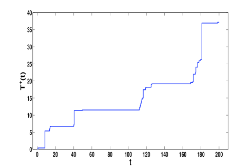
Figure 1: Occupation time of an ACTRW with power law waiting time and Gaussian distribution of step lengths (with zero mean and unit dispersion).
Refer to caption
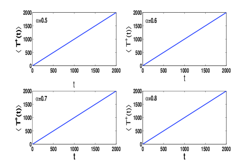
Figure 2: The relation between T+delimited-⟨⟩superscript𝑇\langle T^{+}\rangle and the observation time t𝑡t for various α𝛼\alpha with t>ta𝑡subscript𝑡𝑎t>t_{a}. The number of particles is 400040004000, ta=10subscript𝑡𝑎10t_{a}=10, t=2000𝑡2000t=2000, and α=0.5𝛼0.5\alpha=0.5, 0.60.60.6, 0.70.70.7, and 0.80.80.8. The real lines are obtained by averaging 400040004000 trajectories. It can be noticed that T+delimited-⟨⟩superscript𝑇\langle T^{+}\rangle grows linearly with time t𝑡t.
T+=0tθ(x(τ))𝑑τ,superscript𝑇superscriptsubscript0𝑡𝜃𝑥𝜏differential-d𝜏T^{+}=\int_{0}^{t}\theta(x(\tau))d\tau, (49)

where θ(x)=1𝜃𝑥1\theta(x)=1 for x0𝑥0x\geq 0 and is zeros otherwise. In Fig. 1, we give a trajectory of T+superscript𝑇T^{+} getting from a trajectory of ACTRW model. Furthermore, taking U(x(t))=θ(x(t))𝑈𝑥𝑡𝜃𝑥𝑡U(x(t))=\theta(x(t)), we have the relation A=T+𝐴superscript𝑇A=T^{+}. In order to derive the PDF of T+superscript𝑇T^{+}, we consider the backward Feynman-Kac equation Eq. (47), i.e., power law waiting time and regular jump length, in Laplace space

Gx0(p,s,ta)={Kaω(ta,s)1ω(ta,s)2x02Gx0(p,s,ta)+1s,x0<0;Kaω(ta,s+p)1ω(ta,s+p)2x02Gx0(p,s,ta)+1s+p,x0>0,subscript𝐺subscript𝑥0𝑝𝑠subscript𝑡𝑎casessubscript𝐾𝑎𝜔subscript𝑡𝑎𝑠1𝜔subscript𝑡𝑎𝑠superscript2superscriptsubscript𝑥02subscript𝐺subscript𝑥0𝑝𝑠subscript𝑡𝑎1𝑠x0<0;subscript𝐾𝑎𝜔subscript𝑡𝑎𝑠𝑝1𝜔subscript𝑡𝑎𝑠𝑝superscript2superscriptsubscript𝑥02subscript𝐺subscript𝑥0𝑝𝑠subscript𝑡𝑎1𝑠𝑝x0>0,G_{x_{0}}(p,s,t_{a})=\left\{\begin{array}[]{ll}\frac{K_{a}\omega(t_{a},s)}{1-\omega(t_{a},s)}\frac{\partial^{2}}{\partial x_{0}^{2}}G_{x_{0}}(p,s,t_{a})+\frac{1}{s},&\hbox{$x_{0}<0$;}\\ \frac{K_{a}\omega(t_{a},s+p)}{1-\omega(t_{a},s+p)}\frac{\partial^{2}}{\partial x_{0}^{2}}G_{x_{0}}(p,s,t_{a})+\frac{1}{s+p},&\hbox{$x_{0}>0$,}\end{array}\right. (50)

where Ka=1/2a2subscript𝐾𝑎12superscript𝑎2K_{a}=1/2a^{2} and ω(ta,s)𝜔subscript𝑡𝑎𝑠\omega(t_{a},s) denotes as the PDF of the forward waiting time. From Eq. (22), we obtain

ω(ta,s)=1Γ(α)exp(sta)Γ(α,sta),𝜔subscript𝑡𝑎𝑠1Γ𝛼𝑠subscript𝑡𝑎Γ𝛼𝑠subscript𝑡𝑎\omega(t_{a},s)=\frac{1}{\Gamma(\alpha)}\exp(st_{a})\Gamma(\alpha,st_{a}), (51)

where Γ(α,y)Γ𝛼𝑦\Gamma(\alpha,y) is the incomplete Gamma function Abramowitz1984Handbook and Γ(α,y)=yexp(z)zα1𝑑zΓ𝛼𝑦superscriptsubscript𝑦𝑧superscript𝑧𝛼1differential-d𝑧\Gamma(\alpha,y)=\int_{y}^{\infty}\exp(-z)z^{\alpha-1}dz. Supposing Gx0(p,s,ta)0subscript𝐺subscript𝑥0𝑝𝑠subscript𝑡𝑎0G_{x_{0}}(p,s,t_{a})\rightarrow 0 for |x0|subscript𝑥0|x_{0}|\rightarrow\infty, it’s easy to solve the second order, ordinary differential equation about x0subscript𝑥0x_{0},

Gx0(p,s,ta)={C0exp(x01ω(ta,s)Kaω(ta,s))+1s,x0<0;C1exp(x01ω(ta,s+p)Kaω(ta,s+p))+1s+p,x0>0.subscript𝐺subscript𝑥0𝑝𝑠subscript𝑡𝑎casessubscript𝐶0subscript𝑥01𝜔subscript𝑡𝑎𝑠subscript𝐾𝑎𝜔subscript𝑡𝑎𝑠1𝑠x0<0;subscript𝐶1subscript𝑥01𝜔subscript𝑡𝑎𝑠𝑝subscript𝐾𝑎𝜔subscript𝑡𝑎𝑠𝑝1𝑠𝑝x0>0.G_{x_{0}}(p,s,t_{a})=\left\{\begin{array}[]{ll}C_{0}\exp\Big{(}x_{0}\sqrt{\frac{1-\omega(t_{a},s)}{K_{a}\omega(t_{a},s)}}\Big{)}+\frac{1}{s},&\hbox{$x_{0}<0$;}\\ C_{1}\exp\Big{(}-x_{0}\sqrt{\frac{1-\omega(t_{a},s+p)}{K_{a}\omega(t_{a},s+p)}}\Big{)}+\frac{1}{s+p},&\hbox{$x_{0}>0$.}\end{array}\right. (52)

Here C0subscript𝐶0C_{0} and C1subscript𝐶1C_{1} are undetermined coefficients. It can be noticed the particles can never reach the right plane if the initial position x0subscript𝑥0x_{0}\rightarrow-\infty, i.e., Gx0(T+,t,ta)=δ(T+)subscript𝐺subscript𝑥0superscript𝑇𝑡subscript𝑡𝑎𝛿superscript𝑇G_{x_{0}}(T^{+},t,t_{a})=\delta(T^{+}); furthermore, performing Laplace transform we have Gx0(p,s,ta)=1ssubscript𝐺subscript𝑥0𝑝𝑠subscript𝑡𝑎1𝑠G_{x_{0}}(p,s,t_{a})=\frac{1}{s}, which agrees with Eq. (52). If x0+subscript𝑥0x_{0}\rightarrow+\infty, the probability of the particles to reach the left plane is 00, namely Gx0(T+,t,ta)=δ(T+t)subscript𝐺subscript𝑥0superscript𝑇𝑡subscript𝑡𝑎𝛿superscript𝑇𝑡G_{x_{0}}(T^{+},t,t_{a})=\delta(T^{+}-t) and Gx0(p,s,ta)=1s+psubscript𝐺subscript𝑥0𝑝𝑠subscript𝑡𝑎1𝑠𝑝G_{x_{0}}(p,s,t_{a})=\frac{1}{s+p}, which is consistent with Eq. (52). If assuming that Gx0(p,s,ta)subscript𝐺subscript𝑥0𝑝𝑠subscript𝑡𝑎G_{x_{0}}(p,s,t_{a}) and its first derivative about x0subscript𝑥0x_{0} are continuous at x0=0subscript𝑥00x_{0}=0, we obtain

{C0+1s=C1+1s+pC01ω(ta,s)Kaω(ta,s)=C11ω(ta,s+p)Kaω(ta,s+p).casessubscript𝐶01𝑠subscript𝐶11𝑠𝑝missing-subexpressionsubscript𝐶01𝜔subscript𝑡𝑎𝑠subscript𝐾𝑎𝜔subscript𝑡𝑎𝑠subscript𝐶11𝜔subscript𝑡𝑎𝑠𝑝subscript𝐾𝑎𝜔subscript𝑡𝑎𝑠𝑝absent\left\{\begin{array}[]{ll}C_{0}+\frac{1}{s}=C_{1}+\frac{1}{s+p}&\\ -C_{0}\sqrt{\frac{1-\omega(t_{a},s)}{K_{a}\omega(t_{a},s)}}=C_{1}\sqrt{\frac{1-\omega(t_{a},s+p)}{K_{a}\omega(t_{a},s+p)}}&.\end{array}\right. (53)

From the above equation, there exists

{C0=ps(s+p)(1ω(ta,s+p))ω(ta,s)ω(ta,s+p)(1ω(ta,s))+ω(ta,s)(1ω(ta,s+p)),C1=ps(s+p)(1ω(ta,s))ω(ta,s+p)ω(ta,s+p)(1ω(ta,s))+ω(ta,s)(1ω(ta,s+p)).casessubscript𝐶0𝑝𝑠𝑠𝑝1𝜔subscript𝑡𝑎𝑠𝑝𝜔subscript𝑡𝑎𝑠𝜔subscript𝑡𝑎𝑠𝑝1𝜔subscript𝑡𝑎𝑠𝜔subscript𝑡𝑎𝑠1𝜔subscript𝑡𝑎𝑠𝑝missing-subexpressionsubscript𝐶1𝑝𝑠𝑠𝑝1𝜔subscript𝑡𝑎𝑠𝜔subscript𝑡𝑎𝑠𝑝𝜔subscript𝑡𝑎𝑠𝑝1𝜔subscript𝑡𝑎𝑠𝜔subscript𝑡𝑎𝑠1𝜔subscript𝑡𝑎𝑠𝑝missing-subexpression\left\{\begin{array}[]{ll}C_{0}=-\frac{p}{s(s+p)}\frac{\sqrt{(1-\omega(t_{a},s+p))\omega(t_{a},s)}}{\sqrt{\omega(t_{a},s+p)(1-\omega(t_{a},s))}+\sqrt{\omega(t_{a},s)(1-\omega(t_{a},s+p))}},&\\ C_{1}=\frac{p}{s(s+p)}\frac{\sqrt{(1-\omega(t_{a},s))\omega(t_{a},s+p)}}{\sqrt{\omega(t_{a},s+p)(1-\omega(t_{a},s))}+\sqrt{\omega(t_{a},s)(1-\omega(t_{a},s+p))}}.&\end{array}\right. (54)

For simplicity, let the particle start at x0=0subscript𝑥00x_{0}=0, from Eq. (52) we have G0(p,ta,t)=C0+1/ssubscript𝐺0𝑝subscript𝑡𝑎𝑡subscript𝐶01𝑠G_{0}(p,t_{a},t)=C_{0}+1/s, i.e.,

G0(p,s,ta)=1s(s+p)(p+s)(1ω(ta,s))ω(ta,s+p)+s(1ω(ta,s+p))ω(ta,s)ω(ta,s+p)(1ω(ta,s))+ω(ta,s)(1ω(ta,s+p)).subscript𝐺0𝑝𝑠subscript𝑡𝑎1𝑠𝑠𝑝𝑝𝑠1𝜔subscript𝑡𝑎𝑠𝜔subscript𝑡𝑎𝑠𝑝𝑠1𝜔subscript𝑡𝑎𝑠𝑝𝜔subscript𝑡𝑎𝑠𝜔subscript𝑡𝑎𝑠𝑝1𝜔subscript𝑡𝑎𝑠𝜔subscript𝑡𝑎𝑠1𝜔subscript𝑡𝑎𝑠𝑝\begin{split}G_{0}(p,s,t_{a})=\frac{1}{s(s+p)}\frac{(p+s)\sqrt{(1-\omega(t_{a},s))\omega(t_{a},s+p)}+s\sqrt{(1-\omega(t_{a},s+p))\omega(t_{a},s)}}{\sqrt{\omega(t_{a},s+p)(1-\omega(t_{a},s))}+\sqrt{\omega(t_{a},s)(1-\omega(t_{a},s+p))}}.\end{split} (55)

Especially, if ta=0subscript𝑡𝑎0t_{a}=0, ω(ta=0,t)=ϕ(t)𝜔subscript𝑡𝑎0𝑡italic-ϕ𝑡\omega(t_{a}=0,t)=\phi(t), we have ω(ta=0,s)=ϕ(s)𝜔subscript𝑡𝑎0𝑠italic-ϕ𝑠\omega(t_{a}=0,s)=\phi(s) and ω(ta=0,s+p)=ϕ(s+p)𝜔subscript𝑡𝑎0𝑠𝑝italic-ϕ𝑠𝑝\omega(t_{a}=0,s+p)=\phi(s+p), and Eq. (55) reduces to

G0(p,s)=sα/21+(s+p)α/21sα/2+(s+p)α/2.subscript𝐺0𝑝𝑠superscript𝑠𝛼21superscript𝑠𝑝𝛼21superscript𝑠𝛼2superscript𝑠𝑝𝛼2G_{0}(p,s)=\frac{s^{\alpha/2-1}+(s+p)^{\alpha/2-1}}{s^{\alpha/2}+(s+p)^{\alpha/2}}. (56)

Using the technique given by Godrèche and Luck Godreche2001Statistics , the PDF of y=T+/t𝑦superscript𝑇𝑡y=T^{+}/t can be shown by the Lamperti PDF Carmi2010On , i.e.,

g(y)=sin(πα/2)πyα/21(1y)α/21yα+(1y)α+2yα/2(1y)α/2cos(πα/2).𝑔𝑦𝜋𝛼2𝜋superscript𝑦𝛼21superscript1𝑦𝛼21superscript𝑦𝛼superscript1𝑦𝛼2superscript𝑦𝛼2superscript1𝑦𝛼2𝜋𝛼2\begin{split}g(y)&=\frac{\sin(\pi\alpha/2)}{\pi}\\ &\cdot\frac{y^{\alpha/2-1}(1-y)^{\alpha/2-1}}{y^{\alpha}+(1-y)^{\alpha}+2y^{\alpha/2}(1-y)^{\alpha/2}\cos(\pi\alpha/2)}.\end{split} (57)

For more details, see Godreche2001Statistics ; Lamperti1958An ; Baldassarri1999Statistics . Eq. (55) works well for all time t𝑡t and shows the trend of T+superscript𝑇T^{+}, while it’s difficult to invert Eq. (55) analytically.

IV.2 Fluctuation of occupation fraction

We further introduce η(t)=T+t𝜂𝑡superscript𝑇𝑡\eta(t)=\frac{T^{+}}{t}, a quantity to illustrate the fraction of time that the particle spends within a given domainThaler2002A ; Bel2006Weak ; Godreche2001Statistics . Eq. (55) is very useful to obtain the moments of T+superscript𝑇T^{+}, i.e.,

(T+(s))n=(1)nnpnG0(p,s,ta)|p=0.delimited-⟨⟩superscriptsuperscript𝑇𝑠𝑛evaluated-atsuperscript1𝑛superscript𝑛superscript𝑝𝑛subscript𝐺0𝑝𝑠subscript𝑡𝑎𝑝0\langle(T^{+}(s))^{n}\rangle=(-1)^{n}\frac{\partial^{n}}{\partial p^{n}}G_{0}(p,s,t_{a})|_{p=0}. (58)

From Eq. (55) and Eq. (51), we can obtain

G0(p,s,ta)=1s(s+p)(p+s)(Γ(αestaΓ(α,sta))eptaΓ(α,(s+p)ta)+s(Γ(αe(s+p)taΓ(α,(s+p)ta))Γ(α,sta)(Γ(αestaΓ(α,sta))eptaΓ(α,(s+p)ta)+(Γ(αe(s+p)taΓ(α,(s+p)ta))Γ(α,sta).\begin{split}G_{0}(p,s,t_{a})=\frac{1}{s(s+p)}\frac{(p+s)\sqrt{(\Gamma(\alpha-e^{st_{a}}\Gamma(\alpha,st_{a}))e^{pt_{a}}\Gamma(\alpha,(s+p)t_{a})}+s\sqrt{(\Gamma(\alpha-e^{(s+p)t_{a}}\Gamma(\alpha,(s+p)t_{a}))\Gamma(\alpha,st_{a})}}{\sqrt{(\Gamma(\alpha-e^{st_{a}}\Gamma(\alpha,st_{a}))e^{pt_{a}}\Gamma(\alpha,(s+p)t_{a})}+\sqrt{(\Gamma(\alpha-e^{(s+p)t_{a}}\Gamma(\alpha,(s+p)t_{a}))\Gamma(\alpha,st_{a})}}.\end{split} (59)

Since it is difficult to take inverse transform to Eq. (59) analytically, we just consider the asymptotic behaviors of the moments, inlcuding the first and the second moments of T+superscript𝑇T^{+}. Setting n=1𝑛1n=1 and using the relation between Eq. (58) and Eq. (59), yield

T+(s)=pG0(p,s,ta)|p=0=12s2,delimited-⟨⟩superscript𝑇𝑠evaluated-at𝑝subscript𝐺0𝑝𝑠subscript𝑡𝑎𝑝012superscript𝑠2\langle T^{+}(s)\rangle=-\frac{\partial}{\partial p}G_{0}(p,s,t_{a})|_{p=0}=\frac{1}{2s^{2}}, (60)

by inverse Laplace transform, which leads to

{T+(t)=t/2η(t)=1/2.casesdelimited-⟨⟩superscript𝑇𝑡𝑡2missing-subexpressiondelimited-⟨⟩𝜂𝑡12missing-subexpression\left\{\begin{array}[]{ll}\langle T^{+}(t)\rangle=t/2&\hbox{}\\ \langle\eta(t)\rangle=1/2.&\hbox{}\end{array}\right. (61)

That is to say, for both the weakly and strongly aging systems, the aging time tasubscript𝑡𝑎t_{a} makes no difference to T+(t)delimited-⟨⟩superscript𝑇𝑡\langle T^{+}(t)\rangle. In Fig. 2, we give the simulation results getting from trajectories for ttamuch-greater-than𝑡subscript𝑡𝑎t\gg t_{a}; it can be noticed T+(t)delimited-⟨⟩superscript𝑇𝑡\langle T^{+}(t)\rangle increases linearly with time t𝑡t, which agrees with our theory results Eq. (61). In Laplace space, the second moment of T+(t)superscript𝑇𝑡T^{+}(t) can be given by

T+(s)2=(sta)αestaΓ(α,sta)(4+sta)Γ(α)+4e2staΓ(α,sta)24s3Γ(α,sta)esta(estaΓ(α,sta)Γ(α)).delimited-⟨⟩superscript𝑇superscript𝑠2superscript𝑠subscript𝑡𝑎𝛼superscript𝑒𝑠subscript𝑡𝑎Γ𝛼𝑠subscript𝑡𝑎4𝑠subscript𝑡𝑎Γ𝛼4superscript𝑒2𝑠subscript𝑡𝑎Γsuperscript𝛼𝑠subscript𝑡𝑎24superscript𝑠3Γ𝛼𝑠subscript𝑡𝑎superscript𝑒𝑠subscript𝑡𝑎superscript𝑒𝑠subscript𝑡𝑎Γ𝛼𝑠subscript𝑡𝑎Γ𝛼\begin{split}&\langle T^{+}(s)^{2}\rangle~{}\\ &=\frac{(st_{a})^{\alpha}-e^{st_{a}}\Gamma(\alpha,st_{a})(4+st_{a})\Gamma(\alpha)+4e^{2st_{a}}\Gamma(\alpha,st_{a})^{2}}{4s^{3}\Gamma(\alpha,st_{a})e^{st_{a}}(e^{st_{a}}\Gamma(\alpha,st_{a})-\Gamma(\alpha))}.\end{split} (62)

We first consider weakly aging system, i.e., tatmuch-less-thansubscript𝑡𝑎𝑡t_{a}\ll t. For small y𝑦y, the incomplete Gamma function has the following relation

Γ(α,y)=Γ(α)(1exp(y)n=0yn+αΓ(1+α+n))Γ(α)(1exp(y)yαΓ(1+α)).Γ𝛼𝑦Γ𝛼1𝑦superscriptsubscript𝑛0superscript𝑦𝑛𝛼Γ1𝛼𝑛similar-toΓ𝛼1𝑦superscript𝑦𝛼Γ1𝛼\begin{split}\Gamma(\alpha,y)&=\Gamma(\alpha)\Big{(}1-\exp(-y)\sum_{n=0}^{\infty}\frac{y^{n+\alpha}}{\Gamma(1+\alpha+n)}\Big{)}\\ &\sim\Gamma(\alpha)\Big{(}1-\exp(-y)\frac{y^{\alpha}}{\Gamma(1+\alpha)}\Big{)}.\end{split} (63)

Using Eq. (62) and Eq. (63), for tatmuch-less-thansubscript𝑡𝑎𝑡t_{a}\ll t, i.e., tas0subscript𝑡𝑎𝑠0t_{a}s\rightarrow 0, after a few simple calculations, there exists

T+(s)2(1α/4)s3.similar-todelimited-⟨⟩superscript𝑇superscript𝑠21𝛼4superscript𝑠3\langle T^{+}(s)^{2}\rangle\sim\frac{(1-\alpha/4)}{s^{3}}. (64)

Hence, inverse Laplace transforming Eq. (64) with respect to s𝑠s yields

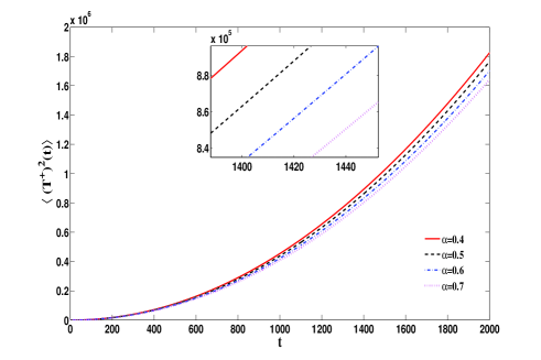
(T+)2(t)(12α8)t2,similar-todelimited-⟨⟩superscriptsuperscript𝑇2𝑡12𝛼8superscript𝑡2\langle(T^{+})^{2}(t)\rangle\sim\left(\frac{1}{2}-\frac{\alpha}{8}\right)t^{2}, (65)

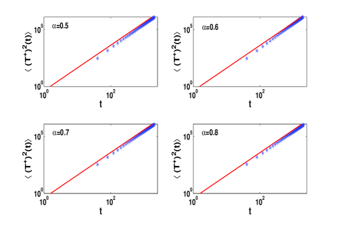
or η(t)2(1/2α/8)similar-todelimited-⟨⟩𝜂superscript𝑡212𝛼8\langle\eta(t)^{2}\rangle\sim(1/2-\alpha/8). In Fig. 3, it can be noticed the theory results are consistent with the simulation results. In addition, the fluctuation of the occupation fraction is

Δη2(t)=η2(t)(η(t))214α8.delimited-⟨⟩subscriptsuperscriptΔ2𝜂𝑡delimited-⟨⟩superscript𝜂2𝑡superscriptdelimited-⟨⟩𝜂𝑡2similar-to14𝛼8\begin{split}\langle\Delta^{2}_{\eta}(t)\rangle&=\langle\eta^{2}(t)\rangle-(\langle\eta(t)\rangle)^{2}\\ &\sim\frac{1}{4}-\frac{\alpha}{8}.\end{split} (66)
Refer to caption
Figure 3: Time evolution of the ensemble average of the occupation time (T+)2(t)delimited-⟨⟩superscriptsuperscript𝑇2𝑡\langle(T^{+})^{2}(t)\rangle with the waiting time PDF Eq. (4) for aging slightly. The parameters are taken as ta=10subscript𝑡𝑎10t_{a}=10, t=2000𝑡2000t=2000, and α=0.5𝛼0.5\alpha=0.5, 0.60.60.6, 0.70.70.7, and 0.80.80.8. The real (red) lines are for the analytical result Eq. (65) and the other symbol lines are obtained by averaging 400040004000 trajectories.

We further consider the strongly aging system, i.e., ttamuch-less-than𝑡subscript𝑡𝑎t\ll t_{a}. For large values of y𝑦y, Γ(α,y)Γ𝛼𝑦\Gamma(\alpha,y) behaves as

Γ(α,y)yα1ey.similar-toΓ𝛼𝑦superscript𝑦𝛼1superscript𝑒𝑦\Gamma(\alpha,y)\sim y^{\alpha-1}e^{-y}. (67)

Substituting Eq. (67) into Eq. (62), there exists

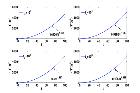
T+(t)2=12t2.delimited-⟨⟩superscript𝑇superscript𝑡212superscript𝑡2\langle T^{+}(t)^{2}\rangle=\frac{1}{2}t^{2}. (68)

Eq. (68) is verified by Fig. 4.

Refer to caption
Figure 4: Time evolution of the ensemble average of the occupation time (T+)2(t)delimited-⟨⟩superscriptsuperscript𝑇2𝑡\langle(T^{+})^{2}(t)\rangle for strongly aging system. The parameters are taken as α=0.6𝛼0.6\alpha=0.6, t=100𝑡100t=100, N=4000𝑁4000N=4000 and ta=103subscript𝑡𝑎superscript103t_{a}=10^{3}, 104superscript10410^{4}, 105superscript10510^{5}, and 106superscript10610^{6}. The solid lines are obtained by averaging 400040004000 trajectories. (T+)2(t)=0.5204t1.976delimited-⟨⟩superscriptsuperscript𝑇2𝑡0.5204superscript𝑡1.976\langle(T^{+})^{2}(t)\rangle=0.5204t^{1.976}, 0.5286t1.9870.5286superscript𝑡1.9870.5286t^{1.987}, 0.51t1.9970.51superscript𝑡1.9970.51t^{1.997}, and 0.4961t1.9990.4961superscript𝑡1.9990.4961t^{1.999} are the fitting results for small t𝑡t and large tasubscript𝑡𝑎t_{a}, which agree with Eq. (68).

Furthermore, we get

Δη2(t)14.similar-todelimited-⟨⟩subscriptsuperscriptΔ2𝜂𝑡14\langle\Delta^{2}_{\eta}(t)\rangle\sim\frac{1}{4}. (69)

From Eq. (69) and Eq. (66), it can be noted that the fluctuation of occupation fraction for strongly aging system is larger than the one of weakly aging system. This can be intuitively explained as follows. For t<<tamuch-less-than𝑡subscript𝑡𝑎t<<t_{a}, i.e, the time t𝑡t is small, the first steps of most particles have not completed and they still stay at the initial position and long waiting time plays an important role. Furthermore, the coefficient of (T+)2(t)delimited-⟨⟩superscriptsuperscript𝑇2𝑡\langle(T^{+})^{2}(t)\rangle increases as the decrease of α𝛼\alpha for weakly aging, which is confirmed by Fig. 5. While, for strongly aging systems, the coefficient of (T+)2(t)delimited-⟨⟩superscriptsuperscript𝑇2𝑡\langle(T^{+})^{2}(t)\rangle is a constant.

Refer to caption
Figure 5: Time evolution of the ensemble average of the occupation time (T+)2(t)delimited-⟨⟩superscriptsuperscript𝑇2𝑡\langle(T^{+})^{2}(t)\rangle for weak aging system. The parameters are taken as ta=2subscript𝑡𝑎2t_{a}=2, t=2000𝑡2000t=2000, and α=0.4𝛼0.4\alpha=0.4, 0.50.50.5, 0.60.60.6, and 0.70.70.7. The symbol lines are obtained by averaging 150001500015000 trajectories.

IV.3 First passage time

First passage times Bel2005Weak ; Buonocore1987A ; Krusemann2014First ; Weihua2017Mean are central features of many families of stochastic processes, including Poisson processes, Wiener processes, gamma processes, and Markov chains, to name but a few. The first passage time, also called the first hitting time, is defined as the time Tfsubscript𝑇𝑓T_{f}, that takes a particle starting at x0=bsubscript𝑥0𝑏x_{0}=-b to hit x=0𝑥0x=0 for the first time with b>0𝑏0b>0. Using the relation between the occupation time functional and the distribution of the first passage time Kac1951On

Pr(Tf>t)=Pr(max0τtx(τ)<0)=limpGx0(p,t,ta),subscript𝑃𝑟subscript𝑇𝑓𝑡subscript𝑃𝑟subscript0𝜏𝑡𝑥𝜏0subscript𝑝subscript𝐺subscript𝑥0𝑝𝑡subscript𝑡𝑎P_{r}(T_{f}>t)=P_{r}(\max_{0\leq\tau\leq t}x(\tau)<0)=\lim_{p\rightarrow\infty}G_{x_{0}}(p,t,t_{a}),

where Gx0(p,t,ta)subscript𝐺subscript𝑥0𝑝𝑡subscript𝑡𝑎G_{x_{0}}(p,t,t_{a}) is the Laplace transform of Gx0(T+,t,ta)subscript𝐺subscript𝑥0superscript𝑇𝑡subscript𝑡𝑎G_{x_{0}}(T^{+},t,t_{a}) w.r.t. T+=0tθ(x(t))𝑑tsuperscript𝑇superscriptsubscript0𝑡𝜃𝑥𝑡differential-d𝑡T^{+}=\int_{0}^{t}\theta(x(t))dt. In fact, Pr(max0<τ<tx(τ)<0)=Pr(T+=0)=limT+00T+Gx0(A,t,ta)𝑑Asubscript𝑃𝑟subscript0𝜏𝑡𝑥𝜏0subscript𝑃𝑟superscript𝑇0subscriptsuperscript𝑇0superscriptsubscript0superscript𝑇subscript𝐺subscript𝑥0𝐴𝑡subscript𝑡𝑎differential-d𝐴P_{r}(\displaystyle\max_{0<\tau<t}x(\tau)<0)=P_{r}(T^{+}=0)=\lim_{T^{+}\rightarrow 0}\int_{0}^{T^{+}}G_{x_{0}}(A,t,t_{a})dA; using the initial value theorem of Laplace transform Dyke2014An , there exists

Pr(T+=0)=limpp[0T+Gx0(A,t,ta)𝑑A]=limpGx0(p,t,ta).subscript𝑃𝑟superscript𝑇0subscript𝑝𝑝delimited-[]superscriptsubscript0superscript𝑇subscript𝐺subscript𝑥0𝐴𝑡subscript𝑡𝑎differential-d𝐴subscript𝑝subscript𝐺subscript𝑥0𝑝𝑡subscript𝑡𝑎\begin{split}P_{r}(T^{+}=0)&=\lim_{p\rightarrow\infty}p\mathcal{L}\left[\int_{0}^{T^{+}}G_{x_{0}}(A,t,t_{a})dA\right]\\ &=\lim_{p\rightarrow\infty}G_{x_{0}}(p,t,t_{a}).\end{split}

Supposing x0=bsubscript𝑥0𝑏x_{0}=-b and p𝑝p\rightarrow\infty, from Eqs. (50) and (54), we can obtain

limpGx0(p,s,ta)=limp1sps(s+p)Γ(α)e(s+p)taΓ(α,(s+p)ta)Γ(α,sta)ebΓ(α)estaΓ(α,sta)KaestaΓ(α,sta)Γ(α)e(s+p)taΓ(α,(s+p)ta)Γ(α,sta)+eptaΓ(α,(s+p)ta)Γ(α)estaΓ(α,sta)Γ(α,sta).subscript𝑝subscript𝐺subscript𝑥0𝑝𝑠subscript𝑡𝑎subscript𝑝1𝑠𝑝𝑠𝑠𝑝Γ𝛼superscript𝑒𝑠𝑝subscript𝑡𝑎Γ𝛼𝑠𝑝subscript𝑡𝑎Γ𝛼𝑠subscript𝑡𝑎superscript𝑒𝑏Γ𝛼superscript𝑒𝑠subscript𝑡𝑎Γ𝛼𝑠subscript𝑡𝑎subscript𝐾𝑎superscript𝑒𝑠subscript𝑡𝑎Γ𝛼𝑠subscript𝑡𝑎Γ𝛼superscript𝑒𝑠𝑝subscript𝑡𝑎Γ𝛼𝑠𝑝subscript𝑡𝑎Γ𝛼𝑠subscript𝑡𝑎superscript𝑒𝑝subscript𝑡𝑎Γ𝛼𝑠𝑝subscript𝑡𝑎Γ𝛼superscript𝑒𝑠subscript𝑡𝑎Γ𝛼𝑠subscript𝑡𝑎Γ𝛼𝑠subscript𝑡𝑎\begin{split}&\lim_{p\rightarrow\infty}G_{x_{0}}(p,s,t_{a})\\ &=\lim_{p\rightarrow\infty}\frac{1}{s}-\frac{p}{s(s+p)}\frac{\sqrt{\Gamma(\alpha)-e^{(s+p)t_{a}}\Gamma(\alpha,(s+p)t_{a})\Gamma(\alpha,st_{a})}e^{-b\sqrt{\frac{\Gamma(\alpha)-e^{st_{a}}\Gamma(\alpha,st_{a})}{K_{a}e^{st_{a}}\Gamma(\alpha,st_{a})}}}}{\sqrt{\Gamma(\alpha)-e^{(s+p)t_{a}}\Gamma(\alpha,(s+p)t_{a})\Gamma(\alpha,st_{a})}+\sqrt{e^{pt_{a}}\Gamma(\alpha,(s+p)t_{a})\Gamma(\alpha)-e^{st_{a}}\Gamma(\alpha,st_{a})\Gamma(\alpha,st_{a})}}.\end{split} (70)

Using Eq. (67), it yields

limpGx0(p,s,ta)=1s1sexp(bΓ(α)estaΓ(α,sta)KaestaΓ(α,sta)).subscript𝑝subscript𝐺subscript𝑥0𝑝𝑠subscript𝑡𝑎1𝑠1𝑠𝑏Γ𝛼superscript𝑒𝑠subscript𝑡𝑎Γ𝛼𝑠subscript𝑡𝑎subscript𝐾𝑎superscript𝑒𝑠subscript𝑡𝑎Γ𝛼𝑠subscript𝑡𝑎\lim_{p\rightarrow\infty}G_{x_{0}}(p,s,t_{a})=\frac{1}{s}-\frac{1}{s}\exp\Big{(}-b\sqrt{\frac{\Gamma(\alpha)-e^{st_{a}}\Gamma(\alpha,st_{a})}{K_{a}e^{st_{a}}\Gamma(\alpha,st_{a})}}\Big{)}. (71)

According to the definition of the first passage time, we can obtain its corresponding PDF

g(ta,t)=t(1Pr(Tf>t))=tlimpGb(p,t,ta).𝑔subscript𝑡𝑎𝑡𝑡1subscript𝑃𝑟subscript𝑇𝑓𝑡𝑡subscript𝑝subscript𝐺𝑏𝑝𝑡subscript𝑡𝑎g(t_{a},t)=\frac{\partial}{\partial t}(1-P_{r}(T_{f}>t))=-\frac{\partial}{\partial t}\lim_{p\rightarrow\infty}G_{-b}(p,t,t_{a}).

Performing Laplace transform with respect to t𝑡t, leads to

g(ta,s)=exp(bΓ(α)exp(sta)Γ(α,sta)Kaexp(sta)Γ(α,sta)).𝑔subscript𝑡𝑎𝑠𝑏Γ𝛼𝑠subscript𝑡𝑎Γ𝛼𝑠subscript𝑡𝑎subscript𝐾𝑎𝑠subscript𝑡𝑎Γ𝛼𝑠subscript𝑡𝑎g(t_{a},s)=\exp\left(-b\sqrt{\frac{\Gamma(\alpha)-\exp(st_{a})\Gamma(\alpha,st_{a})}{K_{a}\exp(st_{a})\Gamma(\alpha,st_{a})}}\right). (72)

This demonstrates that Eq. (72) is valid for all kinds of s𝑠s and tasubscript𝑡𝑎t_{a}. While, it seems difficult to invert Eq. (72) analytically. In the following, we consider the asymptotic behaviors of the density of the first passage time. For sta0𝑠subscript𝑡𝑎0st_{a}\rightarrow 0, i.e., tatmuch-less-thansubscript𝑡𝑎𝑡t_{a}\ll t, a simple calculation gives

g(ta,s)=exp(b1esta(1esta(sta)αΓ(1+α))Kaesta(1esta(sta)αΓ(1+α)))exp(b1KaΓ(1+α)(sta)α2),𝑔subscript𝑡𝑎𝑠𝑏1superscript𝑒𝑠subscript𝑡𝑎1superscript𝑒𝑠subscript𝑡𝑎superscript𝑠subscript𝑡𝑎𝛼Γ1𝛼subscript𝐾𝑎superscript𝑒𝑠subscript𝑡𝑎1superscript𝑒𝑠subscript𝑡𝑎superscript𝑠subscript𝑡𝑎𝛼Γ1𝛼similar-to𝑏1subscript𝐾𝑎Γ1𝛼superscript𝑠subscript𝑡𝑎𝛼2\begin{split}g(t_{a},s)&=\exp\left(-b\sqrt{\frac{1-e^{st_{a}}(1-e^{-st_{a}}\frac{(st_{a})^{\alpha}}{\Gamma(1+\alpha)})}{K_{a}e^{st_{a}}\left(1-e^{-st_{a}}\frac{(st_{a})^{\alpha}}{\Gamma(1+\alpha)}\right)}}\right)\\ &\sim\exp\left(-b\sqrt{\frac{1}{K_{a}\Gamma(1+\alpha)}}(st_{a})^{\frac{\alpha}{2}}\right),\end{split} (73)

which yields

g(ta,t)Γ(1+α)Ka2αtab2αα2(Γ(1+α)Ka2αb2αtta),similar-to𝑔subscript𝑡𝑎𝑡superscriptΓ1𝛼subscript𝐾𝑎2𝛼subscript𝑡𝑎superscript𝑏2𝛼subscript𝛼2superscriptΓ1𝛼subscript𝐾𝑎2𝛼superscript𝑏2𝛼𝑡subscript𝑡𝑎g(t_{a},t)\sim\frac{\sqrt{\Gamma(1+\alpha)K_{a}}^{\frac{2}{\alpha}}}{t_{a}b^{\frac{2}{\alpha}}}\ell_{\frac{\alpha}{2}}\Big{(}\frac{\sqrt{\Gamma(1+\alpha)K_{a}}^{\frac{2}{\alpha}}}{b^{\frac{2}{\alpha}}}\frac{t}{t_{a}}\Big{)}, (74)

with α(t)subscript𝛼𝑡\ell_{\alpha}(t) being the one sided Lévy distribution Klafter2011First , and in Laplace space, 0exp(st)α(t)𝑑t=exp(sα)superscriptsubscript0𝑠𝑡subscript𝛼𝑡differential-d𝑡superscript𝑠𝛼\int_{0}^{\infty}\exp(-st)\ell_{\alpha}(t)dt=\exp(-s^{\alpha}) for s>0𝑠0s>0. For large values of tta𝑡subscript𝑡𝑎\frac{t}{t_{a}}, g(ta,t)𝑔subscript𝑡𝑎𝑡g(t_{a},t) falls off as a power law

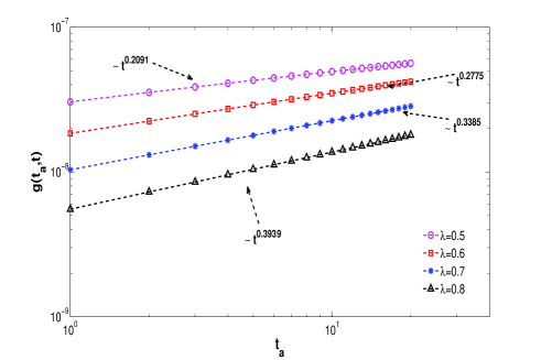
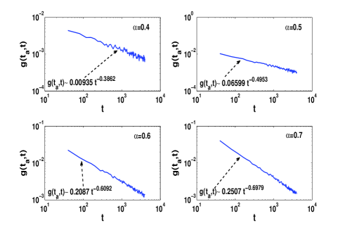
g(ta,t)taα2t1α2,similar-to𝑔subscript𝑡𝑎𝑡superscriptsubscript𝑡𝑎𝛼2superscript𝑡1𝛼2g(t_{a},t)\sim t_{a}^{\frac{\alpha}{2}}t^{-1-\frac{\alpha}{2}}, (75)

which is confirmed by Fig. 6. For small tasubscript𝑡𝑎t_{a} and large t𝑡t, g(ta,t)t1α/2similar-to𝑔subscript𝑡𝑎𝑡superscript𝑡1𝛼2g(t_{a},t)\sim t^{-1-\alpha/2} and g(ta,t)𝑔subscript𝑡𝑎𝑡g(t_{a},t) tends to 00 slowly, which is the same as the behaviors of none aging systemsBarkai2001Fractional .
Refer to caption
Figure 6: Behaviors of first passage time density g(ta,t)𝑔subscript𝑡𝑎𝑡g(t_{a},t) generated by the trajectories of particles for constant jumping length with ta=10subscript𝑡𝑎10t_{a}=10, t=4000𝑡4000t=4000, b=0.05𝑏0.05b=0.05 and α=0.4𝛼0.4\alpha=0.4, 0.50.50.5, 0.60.60.6, and 0.70.70.7. The solid lines are obtained by averaging 106superscript10610^{6} trajectories and the formulaes are the fitting results.
Refer to caption
Figure 7: The relation between first passage time density and tasubscript𝑡𝑎t_{a} for weakly aging system. The parameters are taken as ta=20subscript𝑡𝑎20t_{a}=20, t=106𝑡superscript106t=10^{6}, b=0.05𝑏0.05b=0.05 and α=0.5𝛼0.5\alpha=0.5, 0.60.60.6, 0.70.70.7, and 0.80.80.8. The symbol lines are obtained by the inversion of Eq.  (73). The formulaes are the fitting results for α=0.5𝛼0.5\alpha=0.5, 0.60.60.6, 0.70.70.7, and 0.80.80.8, respectively.

While, if sta𝑠subscript𝑡𝑎st_{a}\rightarrow\infty, corresponding to ttamuch-less-than𝑡subscript𝑡𝑎t\ll t_{a}, from Eq.  (72), we have

g(ta,s)exp(bΓ(α)Kataα1s1α2).similar-to𝑔subscript𝑡𝑎𝑠𝑏Γ𝛼subscript𝐾𝑎superscriptsubscript𝑡𝑎𝛼1superscript𝑠1𝛼2g(t_{a},s)\sim\exp\left(-b\sqrt{\frac{\Gamma(\alpha)}{K_{a}t_{a}^{\alpha-1}}}s^{\frac{1-\alpha}{2}}\right). (76)

Taking the inversion of Eq. (76), there exists

g(ta,t)((KabΓ(α))21α/ta)1α2((KabΓ(α))21αtta).similar-to𝑔subscript𝑡𝑎𝑡superscriptsubscript𝐾𝑎𝑏Γ𝛼21𝛼subscript𝑡𝑎subscript1𝛼2superscriptsubscript𝐾𝑎𝑏Γ𝛼21𝛼𝑡subscript𝑡𝑎g(t_{a},t)\sim\Big{(}\Big{(}\frac{\sqrt{K_{a}}}{b\sqrt{\Gamma(\alpha)}}\Big{)}^{\frac{2}{1-\alpha}}/t_{a}\Big{)}\ell_{\frac{1-\alpha}{2}}\Big{(}\Big{(}\frac{\sqrt{K_{a}}}{b\sqrt{\Gamma(\alpha)}}\Big{)}^{\frac{2}{1-\alpha}}\frac{t}{t_{a}}\Big{)}. (77)

Keeping in mind that t/ta𝑡subscript𝑡𝑎t/t_{a} is a small number, therefore, we can not expand α(t)subscript𝛼𝑡\ell_{\alpha}(t) as tα1superscript𝑡𝛼1t^{-\alpha-1} to obtain its asymptotic form. By numerically inverting Eq. (76) and combining with the form of Eq. (77), we predict that

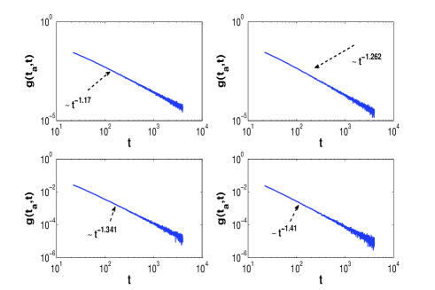
g(ta,t)taα1tα.similar-to𝑔subscript𝑡𝑎𝑡superscriptsubscript𝑡𝑎𝛼1superscript𝑡𝛼g(t_{a},t)\sim t_{a}^{\alpha-1}t^{-\alpha}. (78)

Eq. (78) is confirmed by the simulation of trajectories of the particles; see Fig. 8.
Refer to caption
Figure 8: First passage time density for strongly aging system. The parameters are taken as ta=105subscript𝑡𝑎superscript105t_{a}=10^{5}, t=4000𝑡4000t=4000, b=0.05𝑏0.05b=0.05 and α=0.4𝛼0.4\alpha=0.4, 0.50.50.5, 0.60.60.6, and 0.70.70.7. The solid lines are obtained by averaging 2×1052superscript1052\times 10^{5} trajectories. The formulaes in the lower-left corner of subplots are the fitting results for α=0.4𝛼0.4\alpha=0.4, 0.50.50.5, 0.60.60.6, and 0.70.70.7, respectively.

From Eq. (75) and (78), we can find that the aging times play an important role for the first passage time. For the weakly aging system, the scaling exponent of t𝑡t is 1α21𝛼2-1-\frac{\alpha}{2}, which changes to α𝛼-\alpha for strong aging system. While, for the weakly aging system, the power of tasubscript𝑡𝑎t_{a} is α𝛼\alpha, which becomes α1𝛼1\alpha-1 for strongly aging system.

V SUMMARY AND DISCUSSION

The functionals of the trajectories of particles are very general statistical observables characterizing the motion of particles. In this paper, based on the ACTRW, we derive the forward and backward Feynman-Kac equations governing the distribution of the functionals of the trajectories of particles performing anomalous diffusion with (tempered) power law waiting time and/or jump length distributions. For deep studying the aging phenomena of anomalous diffusion, according to the built models, we more specifically calculate the statistical observables: fraction of the occupation time; first passage time. The fluctuation of the occupation fraction is also analyzed, discovering that the aging time has no influence on its first moment but greatly impacts the second moment. Another striking discovery is for the distribution of the first passage time g(ta,t)𝑔subscript𝑡𝑎𝑡g(t_{a},t), which shows that for slightly (none) aging systems, g(ta,t)taα2t1α2similar-to𝑔subscript𝑡𝑎𝑡superscriptsubscript𝑡𝑎𝛼2superscript𝑡1𝛼2g(t_{a},t)\sim t_{a}^{\frac{\alpha}{2}}t^{-1-\frac{\alpha}{2}}, while for strongly aging systems, g(ta,t)taα1tαsimilar-to𝑔subscript𝑡𝑎𝑡superscriptsubscript𝑡𝑎𝛼1superscript𝑡𝛼g(t_{a},t)\sim t_{a}^{\alpha-1}t^{-\alpha}.

Acknowledgments

This work was supported by the National Natural Science Foundation of China under Grant No. 11671182, and the Fundamental Research Funds for the Central Universities under Grant No. lzujbky-2017-it57 and lzujbky-2017-ot10.

Appendix A Backward Feynman-Kac equation with power law jump length

Here we derive the backward Feynman-Kac equation, and the functional is not necessary positive. From the definition of ACTRW model, the particle waits a time τ𝜏\tau at the position of x0subscript𝑥0x_{0} with the waiting time PDF ω(ta,τ)𝜔subscript𝑡𝑎𝜏\omega(t_{a},\tau), then moves to x0+Δxsubscript𝑥0Δ𝑥x_{0}+\Delta x, the PDF of ΔxΔ𝑥\Delta x being f(Δx)𝑓Δ𝑥f(\Delta x). For simplicity, supposing f(Δx)𝑓Δ𝑥f(\Delta x) has the asymptotic behavior of power law, i.e., f(Δx)|Δx|β1similar-to𝑓Δ𝑥superscriptΔ𝑥𝛽1f(\Delta x)\sim|\Delta x|^{-\beta-1}, there exists

Gx0(A,t,ta)=0tω(ta,t)f(Δx)Gx0+Δx(AτU(x0),tτ,ta)dΔxdτ+(10tω(ta,τ)𝑑τ)δ(AtU(x0)).subscript𝐺subscript𝑥0𝐴𝑡subscript𝑡𝑎superscriptsubscript0𝑡𝜔subscript𝑡𝑎𝑡superscriptsubscript𝑓Δ𝑥subscript𝐺subscript𝑥0Δ𝑥𝐴𝜏𝑈subscript𝑥0𝑡𝜏subscript𝑡𝑎𝑑Δ𝑥𝑑𝜏1superscriptsubscript0𝑡𝜔subscript𝑡𝑎𝜏differential-d𝜏𝛿𝐴𝑡𝑈subscript𝑥0\begin{split}G_{x_{0}}(A,t,t_{a})&=\int_{0}^{t}\omega(t_{a},t)\int_{-\infty}^{\infty}f(\Delta x)\\ &G_{x_{0}+\Delta x}(A-\tau U(x_{0}),t-\tau,t_{a})d\Delta xd\tau\\ &+\Big{(}1-\int_{0}^{t}\omega(t_{a},\tau)d\tau\Big{)}\delta(A-tU(x_{0})).\end{split} (79)

Performing Fourier transform with respect to A𝐴A leads to

Gx0(p,t,ta)=0tω(ta,t)exp(iptU(x0))f(Δx)Gx0+Δx(p,tτ,ta)𝑑Δx𝑑τ+(10tω(ta,τ)𝑑τ)exp(iptU(x0)).subscript𝐺subscript𝑥0𝑝𝑡subscript𝑡𝑎superscriptsubscript0𝑡𝜔subscript𝑡𝑎𝑡superscriptsubscript𝑖𝑝𝑡𝑈subscript𝑥0𝑓Δ𝑥subscript𝐺subscript𝑥0Δ𝑥𝑝𝑡𝜏subscript𝑡𝑎differential-dΔ𝑥differential-d𝜏1superscriptsubscript0𝑡𝜔subscript𝑡𝑎𝜏differential-d𝜏𝑖𝑝𝑡𝑈subscript𝑥0\begin{split}G_{x_{0}}(p,t,t_{a})=\int_{0}^{t}\omega(t_{a},t)\int_{-\infty}^{\infty}\exp(iptU(x_{0}))f(\Delta x)G_{x_{0}+\Delta x}(p,t-\tau,t_{a})d\Delta xd\tau+\Big{(}1-\int_{0}^{t}\omega(t_{a},\tau)d\tau\Big{)}\exp(iptU(x_{0})).\end{split} (80)

Then by Laplace and Fourier transform, we have

Gk0(p,s,ta)=ω(ta,sipU(ik0))f(k0)Gk0(p,s,ta)+1ω(ta,sipU(ik0))sipU(ik0)δ(k0).subscript𝐺subscript𝑘0𝑝𝑠subscript𝑡𝑎𝜔subscript𝑡𝑎𝑠𝑖𝑝𝑈𝑖subscript𝑘0𝑓subscript𝑘0subscript𝐺subscript𝑘0𝑝𝑠subscript𝑡𝑎1𝜔subscript𝑡𝑎𝑠𝑖𝑝𝑈𝑖subscript𝑘0𝑠𝑖𝑝𝑈𝑖subscript𝑘0𝛿subscript𝑘0\begin{split}G_{k_{0}}(p,s,t_{a})&=\omega\Big{(}t_{a},s-ipU\Big{(}-i\frac{\partial}{\partial k_{0}}\Big{)}\Big{)}f(k_{0})G_{k_{0}}(p,s,t_{a})+\frac{1-\omega(t_{a},s-ipU(-i\frac{\partial}{\partial k_{0}}))}{s-ipU(-i\frac{\partial}{\partial k_{0}})}\delta(k_{0}).\end{split} (81)

Rearranging Eq. (81), yields

(sipU(ik0))Gk0(p,s,ta)=(sipU(ik0))ω(ta,sipU(ik0))f(k0)Gk0(p,s,ta)+(1ω(ta,sipU(ik0)))δ(k0).𝑠𝑖𝑝𝑈𝑖subscript𝑘0subscript𝐺subscript𝑘0𝑝𝑠subscript𝑡𝑎𝑠𝑖𝑝𝑈𝑖subscript𝑘0𝜔subscript𝑡𝑎𝑠𝑖𝑝𝑈𝑖subscript𝑘0𝑓subscript𝑘0subscript𝐺subscript𝑘0𝑝𝑠subscript𝑡𝑎1𝜔subscript𝑡𝑎𝑠𝑖𝑝𝑈𝑖subscript𝑘0𝛿subscript𝑘0\begin{split}\Big{(}s-ipU\Big{(}-i\frac{\partial}{\partial k_{0}}\Big{)}\Big{)}G_{k_{0}}(p,s,t_{a})&=\Big{(}s-ipU\Big{(}-i\frac{\partial}{\partial k_{0}}\Big{)}\Big{)}\omega\Big{(}t_{a},s-ipU\Big{(}-i\frac{\partial}{\partial k_{0}}\Big{)}\Big{)}f(k_{0})G_{k_{0}}(p,s,t_{a})\\ &+\Big{(}1-\omega\Big{(}t_{a},s-ipU\Big{(}-i\frac{\partial}{\partial k_{0}}\Big{)}\Big{)}\Big{)}\delta(k_{0}).\end{split} (82)

Performing inverse transform, we obtain the final result

tGx0(p,t,ta)=t(exp(iptU(x0))ω(ta,t))(1+Aβx0β)Gx0(p,t,ta)+ipU(x0)Gx0(p,t,ta)ipU(x0)(exp(iptU(x0))ω(ta,t))(1+Aβx0β)Gx0(p,t,ta)exp(iptU(x0))ω(ta,t),𝑡subscript𝐺subscript𝑥0𝑝𝑡subscript𝑡𝑎𝑡𝑖𝑝𝑡𝑈subscript𝑥0𝜔subscript𝑡𝑎𝑡1subscript𝐴𝛽superscriptsubscriptsubscript𝑥0𝛽subscript𝐺subscript𝑥0𝑝𝑡subscript𝑡𝑎𝑖𝑝𝑈subscript𝑥0subscript𝐺subscript𝑥0𝑝𝑡subscript𝑡𝑎𝑖𝑝𝑈subscript𝑥0𝑖𝑝𝑡𝑈subscript𝑥0𝜔subscript𝑡𝑎𝑡1subscript𝐴𝛽superscriptsubscriptsubscript𝑥0𝛽subscript𝐺subscript𝑥0𝑝𝑡subscript𝑡𝑎𝑖𝑝𝑡𝑈subscript𝑥0𝜔subscript𝑡𝑎𝑡\begin{split}\frac{\partial}{\partial t}G_{x_{0}}(p,t,t_{a})=&\frac{\partial}{\partial t}\Big{(}\exp(iptU(x_{0}))\omega(t_{a},t)\Big{)}*\Big{(}1+A_{\beta}\nabla_{x_{0}}^{\beta}\Big{)}G_{x_{0}}(p,t,t_{a})+ipU(x_{0})G_{x_{0}}(p,t,t_{a})\\ &-ipU(x_{0})\Big{(}\exp(iptU(x_{0}))\omega(t_{a},t)\Big{)}*\Big{(}1+A_{\beta}\nabla_{x_{0}}^{\beta}\Big{)}G_{x_{0}}(p,t,t_{a})-\exp(iptU(x_{0}))\omega(t_{a},t),\end{split} (83)

where x0βsubscriptsuperscript𝛽subscript𝑥0\nabla^{\beta}_{x_{0}} is the Riesz operator, in Fourier space, defined as, [xβg(x)]=|k|βg(k)delimited-[]superscriptsubscript𝑥𝛽𝑔𝑥superscript𝑘𝛽𝑔𝑘\mathcal{F}[\nabla_{x}^{\beta}g(x)]=-|k|^{\beta}g(k); compared to Eq. (48), Eq. (83) is a more general result. In particular, if β=2𝛽2\beta=2, there exists x0β=2x02superscriptsubscriptsubscript𝑥0𝛽superscript2superscriptsubscript𝑥02\nabla_{x_{0}}^{\beta}=\frac{\partial^{2}}{\partial x_{0}^{2}}.

References

  • (1) A. Papoulis, Probability, Random Variables, and Stochastic Processes 2nd ed. (New York: McGraw-Hill, pp. 548-549, 1984).
  • (2) E. Barkai and Y. C. Cheng, J. Chem. Phys. 118, 6167 (2003). 
  • (3) H. Krüsemann, R. Schwarzl, and R. Metzler, Transp. Porous Med. 115, 327 (2016).
  • (4) R. Metzler and J. Klafter, Phys. Rep. 339, 1 (2000).
  • (5) I. Bronstein, Y. Israel, E. Kepten, S. Mai, Y. Shav-Tal, E. Barkai, and Y. Garini, Phys. Rev. Lett. 103, 018102 (2009).
  • (6) R. Nossal, J. Stat. Phys. 30, 391 (1983).
  • (7) G. M. Viswanathan, V. Afanasyev, S. Buldyrev, E. Murphy, P. Prince, H. E. Stanley, et al., Nature 381, 413 (1996).
  • (8) B. O’Shaughnessy and I. Procaccia, Phys. Rev. Lett. 54, 455 (1985).
  • (9) B. B. Mandelbrot and J. W. Van Ness, SIAM Rev. 10, 422 (1968).
  • (10) J. Klafter and I. M. Sokolov, First Steps in Random Walks: From Tools to Applications (Oxford University Press, Oxford, 2011).
  • (11) R. Metzler and J. Klafter, Phys. Rep. 339, 1 (2000).
  • (12) B. J. West and V. Seshadri, Physica A 113, 203 (1982).
  • (13) H. C. Fogedby, Phys. Rev. Lett. 73, 2517 (1994).
  • (14) C. Monthus and J.-P. Bouchaud, J. Phys. A 29, 3847 (1996).
  • (15) E. Marinari and G. Parisi, J. Phys. A 26, L1149 (1993).
  • (16) P. Le Doussal, C. Monthus, and D. S. Fisher, Phys. Rev. E 59, 4795 (1999).
  • (17) I. Sokolov, A. Blumen, and J. Klafter, Phys. A 302, 268 (2001).
  • (18) E. Barkai, Phys. Rev. Lett. 90, 104101 (2003).
  • (19) X. Brokmann, J.-P. Hermier, G. Messin, P. Desbiolles, J.-P. Bouchaud, and M. Dahan, Phys. Rev. Lett. 90, 120601 (2003).
  • (20) L. C. E. Struik, Polym. Eng. Sci. 17, 165 (1977).
  • (21) J. H. P. Schulz, E. Barkai, and R. Metzler, Phys. Rev. Lett. 110, 020602 (2013).
  • (22) A. G. Luchinin and L. S. Dolin, Dokl. Phys. 59, 170 (2014).
  • (23) A. Bar-Haim and J. Klafter, J. Chem. Phys. 109, 5187 (1998).
  • (24) X. H. Wu, W. H. Deng, and E. Barkai, Phys. Rev. E 93, 032151 (2016).
  • (25) D. S. Grebenkov, Rev. Mod. Phys. 79, 1077 (2007).
  • (26) J. Pitman, The Distribution of Local Times of a Brownian Bridge (Springer, Berlin, 1999).
  • (27) M. S. Fischer Black, J. Polit. Econ. 81, 637 (1973).
  • (28) S. N. Majumdar, Current Sci. 89, 2076 (2005).
  • (29) M. Kac, Trans. Amer. Math. Soc. 65, 1 (1949).
  • (30) A. Perret, A. Comtet, S. N. Majumdar, and G. Schehr, J. Stat. Phys. 161, 1112 (2015).
  • (31) A. Baule and R. Friedrich, Phys. Lett. A 350, 167 (2006).
  • (32) S. N. Majumdar and A. J. Bray, Phys. Rev. E 65, 051112 (2002).
  • (33) S. Carmi, L. Turgeman, and E. Barkai, J. Stat. Phys. 141, 1071 (2010).
  • (34) E. W. Montroll and G. H. Weiss, J. Math. Phys. 6, 167 (1965).
  • (35) V. M. Kenkre, E. W. Montroll, and M. F. Shlesinger, J. Stat. Phys. 9, 45 (1973).
  • (36) R. Gorenflo, F. Mainardi, and A. Vivoli, Chaos Solitons Fractals 34, 87 (2007).
  • (37) C. Godrèche and J. M. Luck, J. Stat. Phys. 104, 489 (2001).
  • (38) W. Feller, An Introduction to Probability Theory and Its Applications (John Wiley & Sons, Inc., New York, 1971).
  • (39) P. Dyke, An introduction to Laplace transforms and Fourier series. Springer Undergraduate Mathematics Series (Springer, London, 2014).
  • (40) F. Oberhettinger and L. Badii, Tables of Laplace Transforms (Springer, New York, 1973).
  • (41) A. Erdélyi, W. Magnus, F. Oberhettinger, and F. G. Tricomi, Tables of Integral Transforms (McGraw-Hill Book Company, Inc., New York, 1954).
  • (42) H. Krüsemann, A. Godec, and R. Metzler, Phys. Rev. E 89, 040101 (2014).
  • (43) L. Turgeman, S. Carmi, and E. Barkai, Phys. Rev. Lett. 103, 190201 (2009).
  • (44) A. Compte, Phys. Rev. E 53, 4191 (1996).
  • (45) D. del Castillo-Negrete, Phys. Rev. E 79, 031120 (2009).
  • (46) I. Sokolov, A. Chechkin, and J. Klafter, Phys. A 336, 245 (2004).
  • (47) M. M. Meerschaert, Y. Zhang, and B. Baeumer, Geophys. Res. Lett. 35, L17403 (2008).
  • (48) R. Bruno, L. Sorriso-Valvo, V. Carbone, and B. Bavassano, Europhys. Lett. 66, 146 (2004).
  • (49) R. Weron, Math. Methods Oper. Res. 69, 457 (2009).
  • (50) J. Rosiński, Stochastic Process. Appl. 117, 677 (2007).
  • (51) P. Allegrini, G. Aquino, P. Grigolini, L. Palatella, and A. Rosa, Phys. Rev. E 68, 056123 (2003).
  • (52) W. H. Deng, W. L. Wang, X. C. Tian, and Y. J. Wu, J. Stat. Phys. 164, 377 (2016).
  • (53) S. Redner, A Guide to First-Passage Processes (Cambridge University Press, Cambridge, 2001).
  • (54) E. Barkai, J. Stat. Phys. 123, 883 (2006).
  • (55) S. N. Majumdar and A. Comtet, Phys. Rev. Lett. 89, 060601 (2002).
  • (56) M. Abramowitz and I. A. Stegun (eds.), Handbook of Mathematical Functions with Formulas, Graphs, and Mathematical Tables (John Wiley & Sons, Inc., New York, 1984).
  • (57) J. Lamperti, Trans. Amer. Math. Soc. 88, 380 (1958).
  • (58) A. Baldassarri, J. P. Bouchaud, I. Dornic, and C. Godrèche, Phys. Rev. E 59, R20 (1999).
  • (59) M. Thaler, Ergodic Theory Dynam. Systems 22, 1289 (2002).
  • (60) G. Bel and E. Barkai, Europhys. Lett. 74, 15 (2006).
  • (61) G. Bel and E. Barkai, Phys. Rev. Lett. 94, 240602 (2005).
  • (62) A. Buonocore, A. G. Nobile, and L. M. Ricciardi, Adv. Appl. Probab. 19, 784 (1987).
  • (63) W. H. Deng, X. C. Wu, and W. L. Wang, EPL 117, 10009 (2017).
  • (64) M. Kac, In Proceedings of the Second Berkeley Symposium on Mathematical Statistics and Probability, 189–215 (University of California Press, Berkeley, 1951).
  • (65) E. Barkai, Phys. Rev. E 63, 046118 (2001).

.