Higher-order compatible finite element schemes for the nonlinear rotating shallow water equations on the sphere

Abstract

We describe a compatible finite element discretisation for the shallow water equations on the rotating sphere, concentrating on integrating consistent upwind stabilisation into the framework. Although the prognostic variables are velocity and layer depth, the discretisation has a diagnostic potential vorticity that satisfies a stable upwinded advection equation through a Taylor-Galerkin scheme; this provides a mechanism for dissipating enstrophy at the gridscale whilst retaining optimal order consistency. We also use upwind discontinuous Galerkin schemes for the transport of layer depth. These transport schemes are incorporated into a semi-implicit formulation that is facilitated by a hybridisation method for solving the resulting mixed Helmholtz equation. We demonstrate that our discretisation achieves the expected second order convergence and provide results from some standard rotating sphere test problems.

1 Introduction

The development of new numerical discretisations based on finite element methods is being driven by the need for more flexibility in mesh geometry. The scalability bottleneck arising from the latitude-longitude grid means that weather and climate model developers are searching for numerical discretisations that are stable and accurate on pseudo-uniform grids without sacrificing properties of conservation, balance and wave propagation that are important for accurate atmosphere modelling on the scales relevant to weather and climate (Staniforth and Thuburn, 2012). There is also ongoing interest in adaptively refined meshes as a way of seamlessly coupling global scale and local scale atmosphere simulations, as well as dynamic adaptivity or even moving meshes; using these meshes requires numerical methods that can remain stable and accurate on multiscale meshes. Further, there is an interest in using higher-order spaces to try to offset the inhomogeneity in the error due to using grids that break rotational symmetry.

Compatible finite element methods are a form of mixed finite element methods (meaning that different finite element spaces are used for different fields) that allow the exact representation of the standard vector calculus identities div-curl=0 and curl-grad=0. This necessitates the use of H(div) finite element spaces for velocity, such as Raviart-Thomas and Brezzi-Douglas-Marini, and discontinuous finite element spaces for pressure (stable pairing of velocity and pressure space relies on the existence of bounded commuting projections from continuous to discrete spaces, as detailed in Boffi et al. (2013), for example). The main reason for choosing compatible finite element spaces is that they have a discrete Helmholtz decomposition of the velocity space; this means that there is a clean separation between divergence-free and rotational velocity fields. Cotter and Shipton (2012) used this decomposition to demonstrate that compatible finite element discretisations for the linear shallow water equations on arbitrary grids satisfy the basic conservation, balance and wave propagation properties listed in Staniforth and Thuburn (2012). In particular, it was shown that the discretisation has a geostrophic balancing pressure for every velocity field in the divergence-free subspace of the H(div) finite element space. A survey of the stability and approximation properties of compatible finite element spaces is provided in Natale et al. (2016), including a proof of the absence of spurious inertial oscillations.

The challenge of building atmosphere models using compatible finite elements is that there is no freedom to select finite element spaces in order to ensure good representation of the nonlinear equations (such as conservation, or accurate advection, for example), because the choice has already been made to satisfy linear requirements. In the case of the rotating shallow water equations, the use of discontinuous finite element spaces for the layer depth field encourages us to use upwind discontinuous Galerkin methods, to solve the continuity equation describing layer depth transport.

The nonlinearity in the momentum/velocity equation is more challenging. In McRae and Cotter (2014), the energy-enstrophy conserving formulation of Arakawa and Lamb (1981) was extended to compatible finite element methods. This extension is closely related to C-grid methods for the shallow water equations on more general meshes in Ringler et al. (2010); Thuburn and Cotter (2012). Following these approaches, the compatible finite element formulation, which has velocity and height as prognostic variables, has a diagnostic potential vorticity that satisfies a conservation equation that is implied by the prognostic dynamics for velocity and height. A finite element exterior calculus structure in this formulation was exposed in Cotter and Thuburn (2014), which also provided an alternative formulation based around low-order finite element methods on dual grids. In Thuburn and Cotter (2015), the close relationship of the dual grid formulation to finite volume methods was exploited to obtain a stable discretisation of the nonlinear shallow water equations on the sphere where the finite element formulation of the wave dynamics was coupled with high-order finite volume methods for the layer depth and prognostic potential vorticity fields. The essential idea is to select a particular stable accurate finite volume scheme for the diagnostic potential vorticity, and to then find the update for the prognostic velocity which implies it. In this paper we address the issue of extending this idea to higher-order finite element spaces, for which there is no analogue of the dual grid spaces. This means that we must return to the formulation of McRae and Cotter (2014), where the potential vorticity is stored in a continuous finite element space. We then seek stable accurate higher-order discretisations of the potential vorticity equation using continuous finite element methods that make it possible to find the corresponding update for prognostic velocity. It turns out that this is indeed possible for advection methods from the SUPG/Taylor-Galerkin family of methods.

Finally, we show how these discretisations can be embedded within a semi-implicit time-integration scheme. We again follow the formulation in Thuburn and Cotter (2015), in which advection terms are obtained from explicit time integration methods applied using the (iterative) velocity at time level $n+1/2$. The linear system solved during each nonlinear iteration for the corrections to the field values also requires attention. The standard approach of eliminating velocity to solve a Helmholtz problem for the correction to the layer depth is problematic because the inverse velocity mass matrix is dense. We instead use a hybridised formulation where one solves for the Lagrange multipliers that enforce normal continuity of the velocity field (Boffi et al., 2013, for example).

In section 2 we describe the shallow water model, including the spatial and temporal discretisation; we present finite element spaces that satisfy the properties outlined above and provide details of how to construct such spaces on the sphere and describe advection schemes for both discontinuous and continuous fields as required. In section 3 we present the results of applying our scheme to some of the standard set of test cases for simulation of the rotating shallow water equations on the sphere as described in Williamson et al. (1992) and Galewsky et al. (2004). Section 4 provides a summary and brief outlook.

2 The shallow water model

2.1 Shallow water equations

We begin with the vector invariant form of the nonlinear shallow water equations on a two dimensional surface $\Omega$ embedded in three dimensions,

$$\boldsymbol{u}_{t}+(\zeta+f)\boldsymbol{u}^{\perp}+\nabla\left(g(D+b)+\frac{1}{2}|\boldsymbol{u}|^{2}\right) = 0,$$ (1)

$$D_{t}+\nabla\cdot(\boldsymbol{u}D) = 0,$$ (2)

where $\boldsymbol{u}$ is the horizontal velocity, $D$ is the layer depth, $b$ is the height of the lower boundary, $g$ is the gravitational acceleration, $f$ is the Coriolis parameter and $\zeta=\nabla^{\perp}\cdot\boldsymbol{u}:=(\boldsymbol{k}\times\nabla)\cdot\boldsymbol{u}$ is the vorticity, $\boldsymbol{u}^{\perp}=\boldsymbol{k}\times\boldsymbol{u}$, $\boldsymbol{k}$ is the normal to the surface $\Omega$, and where the $\nabla$ and $\nabla\cdot$ operators are defined intrinsically on the surface. These equations have the important property that the shallow water potential vorticity (PV)

$$q=\frac{\zeta+f}{D}$$ (3)

satisfies a local conservation law,

$$\frac{\partial}{\partial t}(Dq)+\nabla\cdot(\boldsymbol{u}qD)=0.$$ (4)

This can be seen by applying $\nabla^{\perp}\cdot$ to equation (1). Equation (2) then implies that $q$ is constant along characteristics moving with the flow velocity $\boldsymbol{u}$, i.e.,

$$\frac{\partial q}{\partial t}+\left(\boldsymbol{u}\cdot\nabla\right)q=0.$$ (5)

Numerical discretisations that preserve some aspects of these properties have been demonstrated to be very successful at obtaining long time integrations of the rotating shallow water equations on sphere in the quasi-geostrophic flow regime. This is partially because they provide a way to avoid discretising the vector advection term $(\boldsymbol{u}\cdot\nabla)\boldsymbol{u}$ in the velocity equation directly; instead one can choose a suitable stable, accurate and conservative scalar advection scheme for the potential vorticity (treated as a diagnostic variable with $\boldsymbol{u}$ and $D$ being prognostic variables) and use it to diagnose a form of the $(\zeta+f)\boldsymbol{u}^{\perp}$ term in equation (1) that leads to stable advection of $\boldsymbol{u}$. These ideas were introduced in the compatible finite element context in McRae and Cotter (2014) in order to obtain energy-enstrophy conserving discretisations; here we concentrate on stable, accurate and conservative advection of $q$, improving on the low-order APVM stabilisation suggested there. We also replace the centred discretisation of equation (2) with stable and accurate Discontinuous Galerkin (DG) advection schemes for $D$, and show how these can be incorporated into the PV conserving formulation.

2.2 Spatial discretisation

2.2.1 Finite element spaces

In this section we shall summarise the properties we require from our finite element spaces and the operators between them. We start with the space $H(\textrm{div})$ of square integrable velocity fields, whose divergence in also square integrable. The condition that the discrete velocity belongs to the finite element subspace $\mathbb{V}_{1}\subset H(\textrm{div})$ means that the velocity must have continuous normal components across element edges. Having chosen $\mathbb{V}_{1}$, we select a finite element space $\mathbb{V}_{2}\subset L^{2}$ such that

$$\{\nabla\cdot\boldsymbol{w}:\boldsymbol{w}\in\mathbb{V}_{1}\}\subset\mathbb{V}_{2}.$$ (6)

This necessarily requires that $\mathbb{V}_{2}$ is a discontinuous space. We also define a space $\mathbb{V}_{0}\subset H^{1}$ consisting of continuous fields $\gamma$ such that $\boldsymbol{k}\times\nabla\psi\in\mathbb{V}_{1}$, where the curl $\boldsymbol{k}\times\nabla$, henceforth written as $\nabla^{\perp}$, maps from $\mathbb{V}_{0}$ onto the kernel of $\nabla\cdot$ in $\mathbb{V}_{1}$.

The proof that the mixed finite element discretisation of the linear shallow water equations has steady geostrophic modes relies on the existence of a discrete Helmholtz decomposition for the velocity field (Cotter and Shipton, 2012). As described in Arnold et al. (2006), this decomposition exists if the following diagram commutes with bounded projections $\pi_{1}$, $\pi_{2}$, $\pi_{3}$,

$$\begin{CD}H^{1}@>{\nabla^{\perp}}>{}>H(\textrm{div})@>{\nabla\cdot}>{}>L^{2}\\ @V{}V{\pi_{0}}V@V{}V{\pi_{1}}V@V{}V{\pi_{2}}V\\ \mathbb{V}_{0}@>{\nabla^{\perp}}>{}>\mathbb{V}_{1}@>{\nabla\cdot}>{}>\mathbb{V}_{2}\end{CD}$$ (7)

that is, the result of applying an operator to the continuous field and projecting into the discrete space is the same as the result of first projecting the field into the discrete space and then applying the operator.

Cotter and Shipton (2012) reviewed several sets of finite element spaces that satisfy these requirements, together with further requirements on the degree-of-freedom (DOF) ratios between $\mathbb{V}_{1}$ and $\mathbb{V}_{2}$ that are necessary to exclude the possibility of spurious mode branches in the dispersion relation for the linear shallow water equations. In this paper with shall present results from choosing $\mathbb{V}_{1}$ to be the first order Brezzi-Douglas-Marini ($\textrm{BDM}_{2}$) function space on triangles which requires that $\mathbb{V}_{0}$ is $\textrm{P}_{3}$, the space of piecewise continuous cubic functions. $\mathbb{V}_{2}$ is the space $\textrm{P}_{1}^{DG}$ of piecewise linear functions that can be discontinuous at the element boundaries.

2.2.2 Constructing the finite element spaces on the sphere

In order to implement the finite element method, we need to expand our variables in terms of suitable basis functions and compute integrals of combinations of these basis functions over elements. This is done by defining a reference element on which these integrals can be calculated and mappings from each reference element to the physical element, which we describe in this section. A more detailed and general exposition, plus description of how these mappings are implemented in the FEniCS project, is provided in Rognes et al. (2013). In the rest of this section, hatted quantities refer to those defined on the reference element.

We start by defining finite element spaces $\mathbb{V}_{i}(\hat{e})$, $i=0,1,2$, on the reference element $\hat{e}$. These are constructed from polynomials in the usual manner for the chosen spaces as described in Boffi et al. (2013), for example. Then, for each element $e$, we construct a polynomial mapping $\boldsymbol{g}_{e}:\hat{e}\mapsto\mathbb{R}^{3}$, such that

$$\hat{\Omega}=\cup_{i=1}^{N_{e}}\boldsymbol{g}_{e_{i}}(\hat{e}),\quad\boldsymbol{g}_{e_{1}}(\hat{e})\cap\boldsymbol{g}_{e_{2}}(\hat{e})=\emptyset,\,\mbox{ if }e_{1}\neq e_{2},$$ (8)

where $\hat{\Omega}$ is the computational domain, which is a piecewise polynomial approximation to the sphere domain $\Omega$. Then, we use $\boldsymbol{g}_{e}$ to relate functions in our finite element spaces on $\hat{\Omega}$, restricted to each element $e$ in $\hat{\Omega}$, to functions in $\mathbb{V}_{i}(\hat{e})$.

For $\mathbb{V}_{0}$, $\mathbb{V}_{2}$, these functions are simply related by function composition, i.e.,

$$\psi\in\mathbb{V}_{0}\implies\psi|_{e}\circ\boldsymbol{g}_{e}\in\mathbb{V}_{0}(\hat{e}),\quad\phi\in\mathbb{V}_{2}\implies\phi|_{e}\circ\boldsymbol{g}_{e}\in\mathbb{V}_{2}(\hat{e}),$$ (9)

For $\mathbb{V}_{1}$, we use the Piola transformation (Boffi et al., 2013)

$$\boldsymbol{u}|_{e}\left(\boldsymbol{g}_{e}(\hat{\boldsymbol{x}})\right)=\frac{J_{e}\hat{\boldsymbol{u}}}{\det J_{e}},$$ (10)

where $\boldsymbol{u}|_{e}$ is the restriction of $\boldsymbol{u}$ to element $e$, and

$$J_{e}=\frac{\partial\boldsymbol{g}_{e}}{\partial\hat{\boldsymbol{x}}}$$ (11)

is the Jacobian of $\boldsymbol{g}$ in element $e$, to ensure that $\boldsymbol{u}$ is tangent to $\Omega$. The Piola transformation has the crucial property that

$$\nabla\cdot\boldsymbol{u}\left(\boldsymbol{g}_{e}(\hat{\boldsymbol{x}})\right)=\frac{\hat{\nabla}\cdot\hat{\boldsymbol{u}}(\hat{\boldsymbol{x}})}{\det J_{e}\left(\hat{\boldsymbol{x}}\right)}.$$ (12)

When the discrete space is made up of flat elements, as in Cotter and Shipton (2012) and McRae and Cotter (2014), $\det J_{e}$ is constant. This guarantees that if $\hat{\nabla}\cdot\hat{\boldsymbol{u}}\in\hat{\mathbb{V}}_{1}$ then $\nabla\cdot\boldsymbol{u}\in\mathbb{V}_{1}$. However, for meshes made up of general quadrilaterals (i.e. cubed sphere meshes such as those in Putman and Lin (2007)) or high-order, curved triangles, the mapping $\boldsymbol{g}$ is no longer affine and the determinant of its Jacobian is no longer constant. This means that in general $\nabla\cdot\boldsymbol{u}\notin\mathbb{V}_{1}$. This clearly violates the commutative diagram property (7). There are 3 ways to remedy the situation.

1. Modify the mapping for $\mathbb{V}_{2}$ to become

   $$\phi\in\mathbb{V}_{2}\implies\det J_{e}\phi|_{e}\circ\boldsymbol{g}_{e}\in\mathbb{V}_{2}(\hat{e}).$$ (13)

   This option is the choice that is most consistent with the finite element exterior calculus methodology.

2. Modify the mapping for $\mathbb{V}_{1}$ so that the factor of $\det J_{e}$ in $\nabla\cdot\boldsymbol{u}|_{e}\circ\boldsymbol{g}_{e}$ is replaced by the element average of $\det J_{e}$. This approach was described in Boffi and Gastaldi (2009) for the case of lowest order Raviart-Thomas elements; the extension to other H(div) elements is straightforward but the construction is quite complicated.

3. Replace the divergence operator $\nabla\cdot$ in the commutative diagram by $\tilde{\nabla}\cdot$ to be the $L_{2}$ projection $\pi_{2}$ of $\nabla\cdot$ into $\mathbb{V}_{1}$, defined by

   $$\int_{\Omega}\phi\tilde{\nabla}\cdot\boldsymbol{u}\operatorname{d\!}V=\int_{\Omega}\phi\nabla\cdot\boldsymbol{u}\operatorname{d\!}V,\quad\forall\phi\in\mathbb{V}_{2}.$$ (14)

   By defining a new divergence operator in this way we immediately recover the required commutation property, since $\pi_{2}$ appears in the commutative diagram (7) and is a projection. This is a generalisation of the “rehabilitation” technique described for lowest order Raviart-Thomas elements applied to mixed elliptic problems in Bochev and Ridzal (2008). In fact, as Bochev and Ridzal noticed, introduction of the $\tilde{\nabla}\cdot$ operator does not require any changes to a code implementation for mixed elliptic operators since the $\tilde{\nabla}\cdot$ operator only appears in an inner product with a test function from $\mathbb{V}_{2}$, and hence can be safely replaced by $\nabla\cdot$ there. We shall see that this continues to be the case in our nonlinear shallow water formulation.

In general, Option 1 is the most mathematically elegant choice. However, since our software implementation is based upon the Firedrake finite element library (Rathgeber et al., 2016; Luporini et al., 2016) which is already used to develop DG schemes that use the transformations in (9), Option 3 was much less pervasive through the code base. We will investigate the differences between Options 1 and 3 in future work.

Arnold et al. (2014) showed that there is a potential problem with loss of consistency with compatible finite elements on quadrilateral and cubic curvilinear cells; it is likely that this problem also can be exhibited on triangular cells. In particular, for general constructions there may be loss of consistency for the $\mathbb{V}_{1}$ spaces used here (the consistency problem for $\mathbb{V}_{2}$ is avoided through rehabilitation). However, Holst and Stern (2012) demonstrated that consistent approximation can still be obtained if the computational domain can be obtained via a transformation from a mesh of affine elements onto the higher-order nodal interpolation of a $C^{\infty}$ manifold (such as the sphere). This aspect is discussed further in the context of geophysical fluid dynamics in Natale et al. (2016).

2.2.3 Mixed finite element formulation

The mixed finite element discretisation of equations (1)-(2) is formed by restricting $\boldsymbol{u}\in\mathbb{V}_{1}$, $D\in\mathbb{V}_{2}$, multiplying the equations by appropriate test functions, $\boldsymbol{w}\in\mathbb{V}_{1}$ and $\phi\in\mathbb{V}_{2}$, and integrating over the domain, giving

$$\int_{\Omega}\boldsymbol{w}\cdot\boldsymbol{u}_{t}\operatorname{d\!}V+\int_{\Omega}\boldsymbol{w}\cdot\boldsymbol{Q}^{\perp}\operatorname{d\!}V-\int_{\Omega}\nabla\cdot\boldsymbol{w}\left(g\left(D+b\right)+\frac{1}{2}|\boldsymbol{u}|^{2}\right)\operatorname{d\!}V =0,\quad\forall\boldsymbol{w}\in\mathbb{V}_{1},$$ (15)

$$\int_{\Omega}\phi\left(D_{t}+\tilde{\nabla}\cdot\boldsymbol{F}\right)\operatorname{d\!}V =0,\quad\forall\phi\in\mathbb{V}_{2}.$$ (16)

where we have introduced the mass flux $\boldsymbol{F}\in\mathbb{V}_{1}$ (an approximation to $\boldsymbol{u}D$), and the vorticity flux $\boldsymbol{Q}$ (an approximation to $\boldsymbol{u}Dq$). $\boldsymbol{F}$ and $\boldsymbol{Q}$ are defined by appropriate choice of advection schemes for $D$ and the diagnostic potential vorticity $q$, which we shall define later.

We have integrated the gradient term in equation (15) by parts to avoid taking the gradient of the layer depth which is undefined since $D\in\mathbb{V}_{2}$ is discontinuous. A similar problem is posed for the definition of the potential vorticity $q$ since $\zeta=\nabla^{\perp}\cdot\boldsymbol{u}$, which appears in the definition of $q$, is similarly undefined. In order to fix this we integrate the $\nabla^{\perp}$ term by parts (with no surface term since we are solving our equations on the sphere), defining our discrete potential vorticity $q\in\mathbb{V}_{0}$ as

$$\int_{\Omega}\gamma qD\operatorname{d\!}V=\int_{\Omega}-\nabla^{\perp}\gamma\cdot\boldsymbol{u}\operatorname{d\!}V+\int_{\Omega}\gamma f\operatorname{d\!}V\quad\forall\gamma\in\mathbb{V}_{0}.$$ (17)

Provided $D$ remains positive (this can be enforced using a slope limiter, although in the test cases used here the mean depth is sufficiently high that a slope limiter is not required), then this equation can be solved for $q\in\mathbb{V}_{0}$ from known $D$ and $\boldsymbol{u}$. This provides a one-to-one mapping between $q$ and the weak curl of $\boldsymbol{u}$, which leads to a one-to-one mapping between $q$ and the divergence-free part of $\boldsymbol{u}$ via the discrete Helmholtz decomposition (without needing to solve a global Poisson problem). Hence, control of $q$ in the $L^{2}$ norm from a chosen stable advection scheme provides strong control over the divergence-free component of $\boldsymbol{u}$ without compromising the divergent part. This is one reason for the success of this type of potential vorticity conserving discretisation for the rotating shallow water equations.

We differentiate this equation in time, and substitute for $\boldsymbol{u}_{t}$ using equation (15) with $\boldsymbol{w}=-\nabla^{\perp}\gamma$. Since $\nabla\cdot\nabla^{\perp}\equiv 0$ and we assume $f_{t}=0$, this gives

$$\int_{\Omega}\gamma(qD)_{t}\operatorname{d\!}V-\int_{\Omega}\nabla\gamma\cdot\boldsymbol{Q}\operatorname{d\!}V=0,\quad\forall\gamma\in\mathbb{V}_{0},$$ (18)

which is the Galerkin projection of the PV conservation law into $\mathbb{V}_{0}$. If we select $\gamma=1$, then we obtain conservation of total PV,

$$\frac{\operatorname{d\!}}{\operatorname{d\!}t}\int_{\Omega}qD\operatorname{d\!}V=0.$$ (19)

On the other hand, if we are on the sphere, then this quantity is zero as can be computed directly from (17); this topological result stems from the fact that in this case $\boldsymbol{w}=-\nabla{{}^{\perp}}\gamma=0$.

If we choose our advection scheme so that $\boldsymbol{Q}=q\boldsymbol{F}$ and if $q$ is a constant, then we may integrate (18) by parts without introducing error (since $q\in H^{1}$ and $\boldsymbol{F}\in H(\mbox{div})$), and we obtain

$$\int_{\Omega}\gamma(qD)_{t}\operatorname{d\!}V=-\int_{\Omega}\gamma{q}\nabla\cdot(\boldsymbol{F})\operatorname{d\!}V,$$ (20)

and hence

$$\int_{\Omega}\gamma Dq_{t}\operatorname{d\!}V=-\int_{\Omega}\gamma q\left(D_{t}+\nabla\cdot\boldsymbol{F}\right)\operatorname{d\!}V.$$ (21)

For flat elements, or if we had chosen Option 1, the right hand side is zero since $D$ and $\nabla\cdot\boldsymbol{F}$ are in the same finite element space and therefore equation (16) holds pointwise, i.e.,

$$D_{t}+\nabla\cdot\boldsymbol{F}=0.$$ (22)

Hence, we conclude that if $q$ is constant, then $q_{t}=0$, and so $q$ remains constant. As well as being a statement of first-order consistency for the advection scheme for $q$, this is also an important property of equation (5).

The formulation requires some adaptation for the finite element spaces used in this paper to obtain this result, since $\nabla\cdot\boldsymbol{F}$ is not guaranteed to be in the same space as $D$, so equation (22) does not hold pointwise. To recover it, some further “rehabiliation” is required; we amend equation (17) by defining $\tilde{D}\in{\mathbb{V}_{2}}$ such that

$$\frac{\tilde{D}_{t}}{\tau}+\nabla\cdot\boldsymbol{F}=0,$$ (23)

where

$$\tau|_{e}=\det J_{e}\circ g_{e}.$$ (24)

Comparing the weak form of this equation with (16) we see that

$$\int_{\Omega}\phi\frac{\tilde{D}_{t}}{\tau}\operatorname{d\!}V=\int_{\Omega}\phi D_{t}\operatorname{d\!}V\quad\forall\phi\in\mathbb{V}_{2},$$ (25)

which is consistent with the definition

$$\int_{\Omega}\phi\frac{\tilde{D}}{\tau}\operatorname{d\!}V=\int_{\Omega}\phi D\operatorname{d\!}V\quad\forall\phi\in\mathbb{V}_{2},$$ (26)

hence we can solve for $\tilde{D}$ (since $\tau$ is a positive quantity and just alters the metric). $\tilde{D}$ is discontinuous and hence this equation can be solved separately in each element.

Using this in equation (17) gives

$$\int_{\Omega}\gamma q\frac{\tilde{D}}{\tau}\operatorname{d\!}V=-\int_{\Omega}\nabla^{\perp}\gamma\cdot\boldsymbol{u}\operatorname{d\!}V+\int_{\Omega}\gamma f\operatorname{d\!}V\quad\forall\gamma\in\mathbb{V}_{0}.$$ (27)

Differentiating, rearranging and assuming $q$ is constant as before we obtain

$$\int_{\Omega}\gamma\frac{\tilde{D}}{\tau}q_{t}\operatorname{d\!}V=-\int_{\Omega}\gamma q\left(\frac{\tilde{D}{{}_{t}}}{\tau}+\nabla\cdot\boldsymbol{F}\right)\operatorname{d\!}V=0,$$ (28)

as required.

In fact, the finite element formulation allows us to go beyond the first order consistency result. For example, if we choose $\boldsymbol{Q}=\boldsymbol{F}q$, we have enough continuity to integrate by parts, and we obtain

$$\int_{\Omega}\gamma\left((qD)_{t}+\nabla\cdot(\boldsymbol{F}q)\right)\operatorname{d\!}V=0,\quad\forall\gamma\in\mathbb{V}_{0}.$$ (29)

The left-hand side vanishes if $q$ is an exact solution of the equation

$$(qD)_{t}+\nabla\cdot(\boldsymbol{F}q)=0,$$ (30)

where $D$ and $\boldsymbol{F}$ are the discrete mass and mass flux, indicating that the discretisation is consistent at the order of approximation of the finite element space $\mathbb{V}_{0}$. Unfortunately, this is not a good choice for $\boldsymbol{Q}$ since the implied discrete advection operator is not stable. An alternative is to choose

$$\boldsymbol{Q}=\boldsymbol{F}q-\alpha\boldsymbol{F}\frac{\boldsymbol{F}}{|\boldsymbol{F}|}\cdot\nabla q,$$ (31)

where $\alpha$ is a stabilisation parameter. Substitution, rearrangement and integration by parts on the $\boldsymbol{F}q$ term leads to

$$\int_{\Omega}\bigg{(}\gamma+\alpha\frac{\boldsymbol{F}}{|\boldsymbol{F}|}\cdot\nabla{\gamma}\bigg{)}\big{(}(qD)_{t}+\nabla\cdot(\boldsymbol{F}q)\big{)}\operatorname{d\!}V=0,\quad\forall\gamma\in\mathbb{V}_{0},$$ (32)

which is a streamline-upwind Petrov-Galerkin (SUPG) spatial discretisation of the PV conservation equation. This discretisation is stable, and also consistent, i.e. the equation vanishes when the exact solution to (30) is substituted.

In this paper we will use a Taylor-Galerkin discretisation for the potential vorticity equation; this discretisation achieves the same aims as the SUPG discretisation described above, but arises more naturally in the discrete time setting and hence we shall postpone our discussion of it until we have described the time-discrete formulation of the full shallow water system in the next section.

We remark that all of the results above are assuming that integrations are evaluated exactly. Due to the factors of $1/\det J$ arising from the Piola transformation, not all integrands are polynomial and hence exact quadrature is difficult. However, as noted in Cotter and Thuburn (2014), the structure of terms of the following forms,

$$\int_{\Omega}\nabla g\cdot\boldsymbol{v}\operatorname{d\!}x,\quad\int_{\Omega}g\boldsymbol{w}\cdot\boldsymbol{v}^{\perp}\operatorname{d\!}x,\quad\quad\int_{\Omega}g\nabla\cdot\boldsymbol{w}\operatorname{d\!}x,$$ (33)

where $g$ is an arbitrary scalar function (such as a product of scalar functions) and $\boldsymbol{w}$ and $\boldsymbol{v}$ are Piola-mapped functions, means that the factors of $\det J$ cancel after transforming to the reference element, and the integral after change of variables has a polynomial integrand after all. Later on this will also apply to integrals of the form

$$\int_{f}\boldsymbol{v}\cdot\boldsymbol{n}g\operatorname{d\!}S,$$ (34)

where $f$ is an element facet. This means that all of the conservation properties in this paper also hold for inexact quadrature provided that it is sufficiently high order to integrate these polynomial integrands exactly, after appropriately redefining inner products using a quadrature rule instead of an exact integral.

2.3 Time discretisation

We shall build a semi-implicit time discrete formulation. First we write

$$\boldsymbol{u}^{*}=\theta\boldsymbol{u}^{n+1}+(1-\theta)\boldsymbol{u}^{n},D^{*}=\theta D^{n+1}+(1-\theta)D^{n}$$ (35)

and

$$\Delta\boldsymbol{u}=\boldsymbol{u}^{n+1}-\boldsymbol{u}^{n},\Delta D=D^{n+1}-D^{n}.$$ (36)

We can now write equations (15) and (16) as

$$\int_{\Omega}\boldsymbol{w}\cdot\Delta\boldsymbol{u}\operatorname{d\!}V+\Delta t\int_{\Omega}\boldsymbol{w}\cdot\boldsymbol{Q}^{\perp}\operatorname{d\!}V-\Delta t\int_{\Omega}\nabla\cdot\boldsymbol{w}\left(g({D}^{*}+b)+K(\boldsymbol{u}^{*})\right)\operatorname{d\!}V =0,\quad\forall\boldsymbol{w}\in\mathbb{V}_{1},$$ (37)

$$\int_{\Omega}\phi\Delta D\operatorname{d\!}V+\Delta t\int_{\Omega}\phi\nabla\cdot\boldsymbol{F}\operatorname{d\!}V= 0,\quad\forall\phi\in\mathbb{V}_{2},$$ (38)

where

$$K(\boldsymbol{u})=\frac{1}{2}|\boldsymbol{u}|^{2},$$ (39)

and where the time-averaged mass and vorticity fluxes $\boldsymbol{F}$ and $\boldsymbol{Q}$ are yet to be defined. The idea is that we choose $\boldsymbol{F}$ to be a time-independent function such that $D^{n+1}$ is obtained from $D^{n}$ via a high-order stable time discretisation over one timestep for the equation

$$D_{t}+\nabla\cdot(\boldsymbol{u}^{*}D)=0,$$ (40)

i.e. with the advecting velocity frozen to the value of $\boldsymbol{u}^{*}$. Similarly, $\boldsymbol{Q}$ is chosen so that $q^{n+1}$ is related to $q^{n}$ via a high-order stable time discretisation over one timestep for the equation

$$(qD)_{t}+\nabla\cdot(\boldsymbol{F}q)=0,$$ (41)

i.e. with the advecting mass flux frozen to the time-averaged flux $\boldsymbol{F}$. This means that for $\theta=1/2$ we obtain a scheme that is overall second-order in time, but that uses higher-order advection schemes for $D$ and $q$. The rationale is that for near-linear waves, we would like the propagation to be as conservative as possible, so the semi-linear formulation should be based around a time-centred scheme. However, we would also like to obtain good quality solutions over long integrations when close to geostrophic balance, in which case the important quantity is $q$, and it is important that we transport $D$ consistently with $q$ to stay close to the balanced state. In that regime, it is thought to be important to use a high odd-order time integration scheme, since for odd-order schemes the error is dominated by diffusion rather than dispersion (the latter leads to oscillations near to near-discontinuous data). It is also thought that the use of a time-averaged velocity to transport $q$ and $D$ helps to preserve geostrophic balance. This was also the rationale behind choosing the 3rd order Forward-in-Time advection schemes used in Thuburn and Cotter (2015).

An implicit formulation such as the one above requires Newton or Picard iterations to iterate to convergence. In practice, we perform a small fixed number (4) of Picard iterations per timestep, since our aim is to obtain a stable timestepping method with accurate $q$ and $D$ transport, rather than iterating to convergence to obtain an exact implementation of the fully implicit scheme described above. In the Picard iteration we replace the Jacobian obtained from linearisation around the current state with the Jacobian linearised around the system at a state of rest. This means that it is possible to reduce the system as described in the next section, and that the same solver context can be reused during each Picard iteration and timestep.

Hence, each Picard cycle consists of the following steps.

1. Initialise $\Delta\boldsymbol{u}=0$, $\Delta D=0$.

2. Use the current values of $\Delta\boldsymbol{u}$ and $\Delta D$ to compute corresponding values for $\boldsymbol{u}^{*}$, $D^{*}$.

3. Use the chosen mass advection scheme with velocity $\boldsymbol{u}^{*}$ to update from $D^{n}$ to $D^{n+1}$, and find $\boldsymbol{F}$ such that

   $$\int_{\Omega}\phi\left({D}^{n+1}-{D}^{n}+\Delta t\nabla\cdot\boldsymbol{F}\right)\operatorname{d\!}V{=0},\quad\forall\phi\in\mathbb{V}_{2}.$$ (42)

   We will explain how to construct $\boldsymbol{F}$ in section 2.3.2. The mass residual $R_{D}:\mathbb{V}_{2}\to\mathbb{R}$ is defined as

   $$R_{D}[\phi]=\int_{\Omega}\phi(\Delta D+\Delta t\nabla\cdot\boldsymbol{F}{)}\operatorname{d\!}V.$$ (43)

4. Diagnose the PV $q^{n}$ at time $t^{n}$.

5. Use the chosen PV advection scheme with mass flux $\boldsymbol{F}$ to update from $q^{n}$ to $q^{n+1}$ and compute the corresponding PV flux $\boldsymbol{Q}$ such that

   $$\int_{\Omega}\gamma\left(q^{n+1}\frac{\tilde{D}^{n+1}}{\tau}-q^{n}\frac{\tilde{D}^{n}}{\tau}\right)\operatorname{d\!}V-\Delta t\int_{\Omega}\nabla\gamma\cdot\boldsymbol{Q}\operatorname{d\!}V=0,\quad\forall\gamma\in\mathbb{V}_{0}.$$ (44)

6. The velocity residual $R_{\boldsymbol{u}}:\mathbb{V}_{1}\to\mathbb{R}$ is defined as

   $$R_{\boldsymbol{u}}[\boldsymbol{w}]=\int_{\Omega}\boldsymbol{w}\cdot\Delta\boldsymbol{u}\operatorname{d\!}V+\Delta t\int_{\Omega}\boldsymbol{w}\cdot\boldsymbol{Q}{{}^{\perp}}\operatorname{d\!}V+\Delta t\int_{\Omega}\nabla\cdot\boldsymbol{w}\left(g({D}^{*}+b)+K(\boldsymbol{u}^{*})\right)\operatorname{d\!}V.$$ (45)

7. The increments

   $$\Delta\boldsymbol{u}\mapsto\Delta\boldsymbol{u}+\delta\boldsymbol{u},\quad\Delta D\mapsto\Delta D+\delta D$$ (46)

   are then obtained by solving the coupled system

   $$\int_{\Omega}\boldsymbol{w}\cdot\delta\boldsymbol{u}\operatorname{d\!}V+\theta\Delta t\int_{\Omega}f\boldsymbol{w}\cdot\delta\boldsymbol{u}^{\perp}\operatorname{d\!}V-\theta\Delta t\int_{\Omega}\nabla\cdot\boldsymbol{w}g\delta D\operatorname{d\!}V =-R_{\boldsymbol{u}}[\boldsymbol{w}],\quad\forall\boldsymbol{w}\in\mathbb{V}_{1},$$ (47)

   $$\int_{\Omega}\phi\left(\delta D+\theta\Delta tH_{0}\nabla\cdot\delta\boldsymbol{u}\right)\operatorname{d\!}V =-R_{D}[\phi],\quad\forall\phi\in\mathbb{V}_{2},$$ (48)

   where $H_{0}$ is the mean layer depth at rest.

8. If we have not completed 4 iterations, apply these updates and return to 2.

In the following sections we describe the construction of $\boldsymbol{F}$, $\boldsymbol{Q}$ and the solution of the coupled system in detail.

2.3.1 Solving the coupled linear system

In our formulation, we use hybridisation to solve equations ((47)-(48)). Hybridisation is a technique for efficiently solving mixed finite element problems that has been used since the 1960s; in the 1980s it was also discovered that the hybridised formulation could also be used to obtain more accurate approximations of the solution (see Boffi et al. (2013) for a general survey).

Obtaining a hybridised formulation requires two steps. First, we introduce a finite element space $\tilde{\mathbb{V}}_{1}$ by relaxing the normal continuity constraints within $\mathbb{V}_{1}$. In other words, functions in $\tilde{\mathbb{V}}_{1}$ have the same local polynomial representation as functions in $\mathbb{V}_{1}$, but there are no requirements of continuity between edges. In particular, we note that $\mathbb{V}_{1}\subset\tilde{\mathbb{V}}_{1}$. Second, we introduce a trace space $\operatorname{Tr}(\mathbb{V}_{1})$, defined on the element facet set $\Gamma$, such that functions $\lambda\in\operatorname{Tr}(\mathbb{V}_{1})$ are scalar functions which when restricted to a single element facet $f$, are from the same polynomial space as $\boldsymbol{u}\cdot\boldsymbol{n}$ restricted to that facet. Having relaxed the continuity requirements for $\delta\boldsymbol{u}\in\tilde{\mathbb{V}}_{1}$, we enforce them again by adding another equation,

$$\int_{\Gamma}\mu\llbracket\boldsymbol{u}\rrbracket dS=0,\quad\forall\mu\in\operatorname{Tr}(\mathbb{V}_{1}),$$ (49)

where we use the usual “jump” notation

$$\llbracket\boldsymbol{u}\rrbracket=\boldsymbol{u}^{+}\cdot\boldsymbol{n}^{+}+\boldsymbol{u}^{-}\cdot\boldsymbol{n}^{-},$$ (50)

having arbitrarily labelled each side of each facet with $+$ and $-$, so that $\boldsymbol{n}^{+}$ points from the $+$ side to the $-$ side and vice versa. To avoid an over-determined system, we introduce Lagrange multipliers $\lambda\in\operatorname{Tr}(\mathbb{V}_{1})$ and rewrite equations ((47)-(48)) as

$$\int_{\Omega}\boldsymbol{w}\cdot\delta\boldsymbol{u}\operatorname{d\!}V+\theta\Delta t\int_{\Omega}f\boldsymbol{w}\cdot\boldsymbol{u}^{\perp}\operatorname{d\!}V-\theta\Delta t\int_{\Omega}\nabla\cdot\boldsymbol{w}g\delta D\operatorname{d\!}V+\int_{\Gamma}\lambda\llbracket\boldsymbol{w}\rrbracket\operatorname{d\!}S =-R_{\boldsymbol{u}}[\boldsymbol{w}],\quad\forall\boldsymbol{w}\in\tilde{\mathbb{V}}_{1},$$ (51)

$$\int_{\Omega}\phi\left(\delta D+\theta\Delta tH_{0}\nabla\cdot\delta\boldsymbol{u}\right)\operatorname{d\!}V =-R_{D}[\phi],\quad\forall\phi\in\mathbb{V}_{2},$$ (52)

together with equation (49). Note that the residual $R_{\boldsymbol{u}}$ must now be evaluated with $\boldsymbol{w}\in\tilde{\mathbb{V}}_{1}$. All of the inter-element coupling in equations ((51)-(52)) takes place in the $\lambda$ term. This means that if $\lambda$ is known, then it is possible to obtain $\boldsymbol{u}$ and $D$ independently in each element. To enable elimination of $\boldsymbol{u}$ and $D$, we define a lifting operator $L:\operatorname{Tr}(\mathbb{V}_{1})\to\tilde{\mathbb{V}}_{1})$, which gives the solution $\boldsymbol{u}$ for a given $\lambda$ in the case when $R_{D}[\phi]$ and $R_{\boldsymbol{u}}[\boldsymbol{w}]$ are replaced by zero. We also define $\boldsymbol{u}_{0}$ which is the solution obtained when $\lambda$ is zero, but $R_{D}[\phi]$ and $R_{\boldsymbol{u}}[\boldsymbol{w}]$ are present. Then, the general solution of this equation given particular $R_{D}$ and $R_{\boldsymbol{u}}$ is

$$\boldsymbol{u}=L\lambda+\boldsymbol{u}_{0}.$$ (53)

Substituting into equation (49) gives

$$\int_{\Gamma}\mu\llbracket L\lambda\rrbracket\operatorname{d\!}S=-\int_{\Gamma}\mu\llbracket\boldsymbol{u}_{0}\rrbracket\operatorname{d\!}S,\quad\forall\mu\in\operatorname{Tr}(\mathbb{V}_{1}).$$ (54)

This reduced equation can be solved for $\lambda$ before reconstructing $\boldsymbol{u}$ and $D$ by solving equations ((51)-(52)) independently in each element. Since the value of $L\lambda$ in each element only depends on the values of $\lambda$ on the facets of that element, equation (54) only couples together values of $\lambda$ on facets that share an element. This means that the matrix-vector form of this equation is very sparse. In fact, the matrix can be assembled by visiting each element separately, performing inversion on element block systems. Further, this equation has the same spectral properties as the Helmholtz operator, and hence can be solved with Krylov methods and standard preconditioners such as SOR, algebraic multigrid; a geometric multigrid for general higher-order hybridised mixed finite element elliptic problems was provided in Gopalakrishnan and Tan (2009). Note that the Coriolis term can be included in the linear system in this approach without altering the sparsity of the reduced system. One important aspect is that if the solver for this system is not iterated to convergence, the resulting velocity field will not be exactly div-conforming. We address this in our implementation by simply projecting the velocity back into $\mathbb{V}_{1}$ after reconstruction, which appears not to cause any problems with stability. A more sophisticated approach would use the hybridised solver as a preconditioner for the $(\Delta u,\Delta{D})$ system on $(\mathbb{V}_{1},\mathbb{V}_{2})$; we will investigate this in further work.

2.3.2 Advection scheme for layer depth $D$

We now need to solve the mass continuity equation (16) for the update to $D$. As $D\in\mathbb{V}_{2}$ and is therefore discontinuous, we can use standard upwind discontinuous Galerkin methods to obtain an approximation to $D_{t}$,

$$\int_{e}\phi D_{t}\operatorname{d\!}V=\Delta t\int_{e}\nabla\phi\cdot\boldsymbol{u}^{*}{D}\operatorname{d\!}V-\Delta t\int_{\partial e}\phi D^{u}\boldsymbol{u}^{*}\cdot\boldsymbol{n}\operatorname{d\!}S,\quad\forall\phi\in\mathbb{V}_{2}(e),$$ (55)

for each element $e$, where $\mathbb{V}_{1}(e)$ is the space $\mathbb{V}_{1}$ restricted to the element $e$, and $D^{u}$ is the value of $D$ on the upwind side of the element boundary $\partial e$. We then use the standard 3-stage Strong Stability Preserving Runge-Kutta scheme (Gottlieb et al., 2001),

$$D^{1} =D^{n}+\Delta tD_{t}^{n},$$ (56)

$$D^{2} =\frac{3}{4}D^{n}+\frac{1}{4}\left(D^{1}+\Delta tD_{t}^{1}\right),$$ (57)

$$D^{n+1} =\frac{1}{3}D^{n}+\frac{2}{3}\left(D^{2}+\Delta tD_{t}^{2}\right).$$ (58)

Later we shall discuss a consistency property of the potential vorticity conserving discretisation of the velocity equation; this property requires that we find a time-integrated mass flux $\bar{\boldsymbol{F}}\in\mathbb{V}_{1}$ that satisfies

$$\Delta D=-\Delta t\nabla\cdot\bar{\boldsymbol{F}}.$$ (59)

This is done by finding $\boldsymbol{F}$ given $D_{t}$ such that

$$D_{t}+\nabla\cdot\boldsymbol{F}=0,$$ (60)

and then substituting into equations ((56)-(58)) to construct $\bar{\boldsymbol{F}}$. To find a flux $\boldsymbol{F}$ for each Runge-Kutta stage, we solve

$$\int_{f}\kappa\boldsymbol{F}\cdot\boldsymbol{n}\operatorname{d\!}s =\int_{f}\kappa D^{u}\boldsymbol{u}^{*}\cdot\boldsymbol{n}\operatorname{d\!}s \forall\kappa\in\operatorname{Tr}{{}_{f}}(\mathbb{V}_{1}),{\quad\forall f\in\partial e}$$ (61)

$$\int_{e}\boldsymbol{w}\cdot\boldsymbol{F}\operatorname{d\!}x =\int_{e}\boldsymbol{w}\cdot\boldsymbol{u}^{*}D\operatorname{d\!}x \forall\phi\in\mathring{\mathbb{V}}_{1}^{*}(e),$$ (62)

where $\mathring{\mathbb{V}}^{*}_{1}(e)$ is the right size to close the system and $\nabla\phi\in\mathring{{\mathbb{V}}}_{1}^{*}(e)$ for all $\phi\in\mathbb{V}_{2}(e)$. The left-hand sides of equations ((61)-(62)) are the same as the left-hand sides of the definition of the commuting operator $\pi:\operatorname{H(div)}\to\mathbb{V}_{1}$ that features in stability proofs for mixed finite element methods (see Boffi et al. (2013), for example). This means that the above construction is well-posed. To check that equation (60) is satisfied, we integrate (59) by parts. Then, substituting the above relations (61)-(62) (with $\boldsymbol{w}=\nabla\phi)$, we see that

$$\int_{e}\phi D_{t}\operatorname{d\!}V =-\Delta t\int_{e}\phi\nabla\cdot\boldsymbol{F}\operatorname{d\!}V$$

$$=\Delta t\int_{e}\nabla\phi\cdot\boldsymbol{F}\operatorname{d\!}V-\Delta t\int_{\delta e}\phi\boldsymbol{F}\cdot\boldsymbol{n}\operatorname{d\!}S$$

$$=\Delta t\int_{e}\nabla\phi\cdot\boldsymbol{u}^{*}D\operatorname{d\!}V-\Delta t\int_{\delta e}\phi D^{u}\boldsymbol{u}^{*}\cdot\boldsymbol{n}\operatorname{d\!}S,$$

as required.

We note, although we did not use it in this paper, that the use of a slope limiter can also be incorporated into the mass flux computation. If a slope limiter is used after a Runge-Kutta stage, then $D$ is replaced by $D^{\prime}$, with $\int_{e}D-D^{\prime}\operatorname{d\!}x=0$. If we seek $\boldsymbol{F}^{\prime}$ such that

$$D^{\prime}-D+\Delta t\nabla\cdot\boldsymbol{F}^{\prime}=0,$$ (63)

then integration over a single element immediately tells us that this can be satisfied by

$$\int_{f}\kappa\boldsymbol{F}^{\prime}\cdot\boldsymbol{n}\operatorname{d\!}S=0,\quad\forall\kappa\in\operatorname{Tr}{{}_{f}}(\mathbb{V}_{1}),{\quad\forall f\in\partial e},$$ (64)

i.e. $\boldsymbol{F}^{\prime}\cdot\boldsymbol{n}=0$ on the boundary $\partial e$. We then solve a local mixed problem for $(\boldsymbol{F}^{\prime},p)\in(\mathbb{V}_{1}(e),\mathbb{V}_{2}(e))$, given by

$$\int_{e}\phi\nabla\cdot\boldsymbol{F}^{\prime}\operatorname{d\!}x =\int_{e}\phi(D^{\prime}-D)\operatorname{d\!}x,{\quad\forall\phi\in\mathbb{V}_{2}(e)},$$ (65)

$$\int_{e}\boldsymbol{w}\cdot\boldsymbol{F}^{\prime}+\nabla\cdot\boldsymbol{w}p\operatorname{d\!}x =0,{\quad\forall\boldsymbol{w}\in\mathbb{V}_{1}(e)},$$ (66)

subject to the above zero Dirichlet boundary conditions for $\boldsymbol{F}^{\prime}$, where $p$ is introduced to determine a unique $\boldsymbol{F}^{\prime}$.

2.3.3 Advection scheme for velocity $\boldsymbol{u}$

The advection scheme described in this section follows the following design strategy: find an advection scheme for $q$ that is compatible with equation (37), and select the corresponding $\boldsymbol{Q}$ for insertion into that equation to compute $R_{\boldsymbol{u}}[\boldsymbol{w}]$. Selecting $\boldsymbol{w}=-\nabla^{\perp}\gamma$ in equation (37), evaluating equation (17) at time levels $n$ and $n+1$ and substituting gives

$$\int_{\Omega}\gamma q^{n+1}D^{n+1}\operatorname{d\!}x-\int_{\Omega}\gamma q^{n}D^{n}\operatorname{d\!}x-\Delta t\int_{\Omega}\nabla\gamma\cdot\boldsymbol{Q}\operatorname{d\!}x=0,\quad\forall\gamma\in\mathbb{V}^{0},$$ (67)

after noting that $\boldsymbol{w}$ is divergence-free. McRae and Cotter (2014) used $\boldsymbol{Q}=\bar{\boldsymbol{F}}q^{n+1/2}$ to obtain an implicit midpoint rule time discretisation for an energy-enstrophy conserving formulation. In this paper, we aim to use higher-order stabilised advection schemes in order to obtain accurate representation of potential vorticity transport. We note that Streamline Upwind Petrov Galerkin methods (Brooks and Hughes, 1982) and Taylor-Galerkin methods (Donea, 1984) all result in time-discrete formulations equivalent to equation (67).

It is desirable to use a higher order timestepping scheme for $q$, to obtain accurate transport of potential vorticity using the balanced flow. In particular, odd-ordered schemes are attractive since the leading order error is diffusive rather than dispersive. Hence, in this paper we make use of the two-step third-order unconditionally-stable Taylor-Galerkin scheme of Safjan and Oden (1993).

Taylor-Galerkin schemes are built by transforming time derivatives into space derivatives using the advection equation.

The general form of a multistage Taylor-Galerkin method is

$${Z}_{i}-\eta(\Delta t)^{2}(Z_{i})_{tt}=Z^{n}+\Delta t\sum_{j=1}^{i}\mu_{ij}(Z_{j})_{t}+(\Delta t)^{2}\sum_{j=1}^{i}\nu_{ij}(Z_{j})_{tt},\quad i=1,\ldots,k,$$ (68)

where $\eta$ is a stabilisation parameter, the subscript $i$ is the stage index, and the $\{\mu\}_{ij}$ and $\{\nu\}_{ij}$ are coefficients defined in Safjan and Oden (1993). After computing these stage variables, the value of $Z_{k}$ is copied into $Z^{n+1}$.

In our discretisation we use a formulation where $Z=qD$. Then we have

$$\int_{\Omega}\gamma(qD)_{t}\operatorname{d\!}x =\int_{\Omega}\nabla\gamma\cdot\left(\bar{\boldsymbol{F}}q\right)\operatorname{d\!}x,\quad\forall\gamma\in\mathbb{V}_{0},$$ (69)

$$\int_{\Omega}\gamma(qD)_{tt}\operatorname{d\!}x =\int_{\Omega}\nabla\gamma\cdot\left(\bar{\boldsymbol{F}}q_{t}\right)\operatorname{d\!}x=-\int_{\Omega}\nabla\gamma\cdot\left(\bar{\boldsymbol{F}}\frac{\bar{\boldsymbol{F}}}{\bar{D}}\cdot{\nabla}q\right)\operatorname{d\!}x,\quad\forall\gamma\in\mathbb{V}_{0},$$ (70)

recalling that $\bar{F}=\bar{D}\bar{\boldsymbol{u}}$ is considered to be time-independent over the advection step as part of the semi-implicit discretisation. Combination with Equation (68) leads to

$$\int_{\Omega}\gamma q_{i}D^{n+1}+\eta\Delta t^{2}\frac{\bar{\boldsymbol{F}}}{\bar{D}}\cdot\nabla\gamma\bar{\boldsymbol{F}}\cdot\nabla q_{i}\operatorname{d\!}x =\int_{\Omega}\gamma q^{n}D^{n}+\Delta t\sum_{j=1}^{i}\mu_{ij}\int_{\Omega}\nabla\gamma\cdot\bar{\boldsymbol{F}}q_{j}\operatorname{d\!}x-$$

$$\qquad(\Delta t)^{2}\sum_{j=1}^{i}\nu_{ij}\int_{\Omega}\frac{\bar{\boldsymbol{F}}}{\bar{D}}\cdot\nabla\gamma\bar{\boldsymbol{F}}\cdot\nabla q_{j}\operatorname{d\!}x,\quad\forall\gamma\in\mathbb{V}_{0}.$$ (71)

Note that this equation involves solving a Helmholtz-type equation with derivatives in the streamline direction for each stage variable. This equation is symmetric positive definite and well-conditioned for $\mathcal{O}(1)$ Courant numbers; the conjugate gradient method converges quickly with simple SOR preconditioning.

In this paper we took the following coefficients

$$\eta=0.48,\,c_{1}=\frac{1}{2}\left(1+(-\frac{1}{3}+8\eta)^{\frac{1}{2}}\right),\,\mu_{11}=c_{1},\,\mu_{12}=0,\,\mu_{21}=\frac{1}{2}\left(3-\frac{1}{c_{1}}\right),\,$$

$$\mu_{22}=\frac{1}{2}\left(\frac{1}{c_{1}}-1\right),\,\nu_{11}=\frac{1}{2}c_{1}^{2}-\eta,\,\nu_{12}=0,\,\nu_{21}=\frac{1}{4}\left(3c_{1}-1\right)-\eta,\,\nu_{22}=\frac{1}{4}\left(1-c_{1}\right).$$ (72)

Safjan and Oden (1993) showed this scheme to be third order and unconditionally stable for $\eta>0.473$.

Having solved for $q^{n+1}$, we take $i=2$, and notice that equation (71) takes the form of equation (67), and hence $\boldsymbol{Q}$ can be extracted for insertion into equation (37). For the case of curved elements, $D$ must be replaced by $\tilde{D}/\tau$ throughout.

3 Numerical Results

In this section we show numerical results from three standard test cases on icosahedral grids, using the spaces $(P_{3},BDM_{2},DG_{1})$, and a piecewise cubic approximation to the surface of the sphere. The code was implemented using the Firedrake finite element framework, which permits the symbolic implementation of the mixed finite element techniques discussed in this paper. Using the Unified Form Language (see Alnæs et al. (2014)), which provides a high-level mathematical description of the finite element problem, code is automatically generated which forms the resulting matrix equations by assembling the local contributions from each cell and/or facet of the mesh. These equations are provided directly to PETSc (Balay et al., 2016, 1997), which provides direct access to runtime configurable iterative solvers and preconditioners. The hybridisation of the implicit system for the linear updates is implemented using the Slate framework (Gibson et al., 2018), which performs the local elimination and recovery operations. The reduced equation for the trace variables is numerically inverted using the conjugate gradient method and PETSc’s smooth aggregation multigrid preconditioner (GAMG).

The first two test cases are numbers $2$ (solid body rotation) and $5$ (flow over a mountain) from Williamson et al. (1992) and the third is the barotropically unstable jet from Galewsky et al. (2004). Table 1 contains information on the properties of the 4 grids that we use for the Williamson convergence tests, along with the timesteps used. The timestep was chosen to give a constant Courant number across the different resolutions; $0.2$ in the solid body rotation test and $0.06$ in the flow over a mountain test, although we note that in order to see second order convergence, we had to further reduce the timestep for the highest resolution mountain simulation because at this resolution the time discretisation errors start to dominate. Figure 1 shows the lowest resolution icosahedral grid that we use.

Grid properties				DOFs			Test 2	Test 5
cells	nodes	$\Delta x_{\max}$ (km)	$\Delta x_{\min}$ (km)	$\boldsymbol{u}$	$D$	$q$	$\Delta t$ (s)	$\Delta t$ (s)
1280	642	1054	720	9600	3840	5762	3000	$900$[t]
5120	2562	527	348	38400	15360	23042	1500	$450$
20480	10242	263	171	153600	61440	92162	750	$225$
81920	40962	132	85	614400	245760	368642	375	$84.375$

Table 1: Grid properties for the 4 grids used in the convergence tests, including the number of degrees of freedom (DOFs) for velocity $\boldsymbol{u}$, depth $D$ and potential vorticity $q$, along with the timestep used for the solid body rotation test (2) and flow over a mountain test (5).

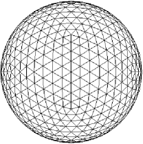
Figure 1: Icosahedral sphere grid, viewed looking down on the North pole, corresponding to the lowest resolution described in table 1.

Where shown, normalised errors in a field $q$ are computed as in Williamson et al. (1992) as

$$L_{2}(q) =\frac{\left(\int_{\Omega}(q-q_{T})^{2}\operatorname{d\!}V\right)^{\frac{1}{2}}}{\left(\int_{\Omega}q_{T}^{2}\operatorname{d\!}V\right)^{\frac{1}{2}}},$$ (73)

$$L_{\infty}(q) =\frac{\max|q-q_{T}|}{\max|q_{T}|},$$ (74)

where $q_{T}$ is the true solution, specified either analytically (as in the solid body rotation test) or from a high resolution reference solution (as in the flow over a mountain test).

3.1 Solid body rotation (Williamson, test case 2)

This test case is initialised with depth and velocity fields that are in geostrophic balance:

$$D =D_{0}-\left(R\Omega u_{0}+\frac{u_{0}^{2}}{2}\right)\frac{z^{2}}{gR^{2}},$$ (75)

$$u =\frac{u_{0}}{R}(-y,x,0),$$ (76)

where $R=6.37122\times 10^{6}\text{m}$ is the radius of the Earth, $\Omega=7.292\times 10^{-5}\text{s}^{-1}$ is the rotation rate of the Earth, $(x,y,z)$ are the $3D$ Cartesian coordinates, $g=9.80616\text{ms}^{-2}$ is the gravitational acceleration, $D_{0}=2.94\times 10^{4}/g\approx 2998\text{m}$ and $u_{0}=2\pi R/(12\text{ days})\approx 38.6\text{ms}^{-1}$. Since there is no topography or other forcing, the flow should remain in this steady, balanced state. As the flow is steady we have an analytic solution which allows us to compute errors and hence an order of convergence for our method. We present these results in table 2 and Figure 2 reveals that our method is converging at second order. The depth error at day 15, shown in Figure 3, is large scale and shows some evidence of grid imprinting.

cells	$L_{2}(D)$	$L_{\infty}(D)$	$L_{2}(\boldsymbol{u})$	$L_{\infty}(\boldsymbol{u})$
1280	$5.929\text{\times}{10}^{-5}$	$2.177\text{\times}{10}^{-4}$	$7.180\text{\times}{10}^{-4}$	$1.701\text{\times}{10}^{-3}$
5120	$9.154\text{\times}{10}^{-6}$	$4.405\text{\times}{10}^{-5}$	$1.261\text{\times}{10}^{-4}$	$2.978\text{\times}{10}^{-4}$
20480	$1.840\text{\times}{10}^{-6}$	$1.062\text{\times}{10}^{-5}$	$2.761\text{\times}{10}^{-5}$	$6.588\text{\times}{10}^{-5}$
81920	$4.288\text{\times}{10}^{-7}$	$2.636\text{\times}{10}^{-6}$	$6.640\text{\times}{10}^{-6}$	$1.551\text{\times}{10}^{-5}$

Table 2: Normalised depth, $D$, and velocity, $\boldsymbol{u}$, errors at day 15 for the solid body rotation test case.

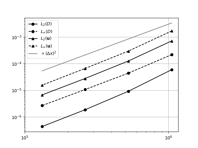
Figure 2: Solid body rotation test case: normalised depth, $D$, and velocity, $\boldsymbol{u}$, errors at day 15 versus average mesh size $\Delta x$.

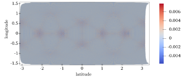
Figure 3: Solid body rotation test case: depth error (in metres) at day 15. The range is min:$-5.8\text{\times}{10}^{-3}$m, max: $7.9\text{\times}{10}^{-3}$m.

3.2 Flow over a mountain (Williamson, test case 5)

This test case uses the same zonal flow initial conditions (75)-(76) as the previous test but with $D_{0}=5960\text{m}$ and $u_{0}=20\text{m}$. An isolated, conical mountain, given by

$$D_{s}=D_{s0}(1-r/R_{0})$$ (77)

with $D_{s0}=2000\text{m}$, $R_{0}=\pi/9$ and $r^{2}=\min[R_{0}^{2},(\phi-\phi_{c})^{2}+(\lambda-\lambda_{c})^{2}]$ is placed with its centre at latitude $\phi=\pi/6$ and longitude $\lambda=-\pi/2$. As the zonal flow interacts with the mountain, it produces waves that travel around the globe. As there is no analytical solution for this problem, the model output at 15 days is compared to a high resolution (a 2048 by 1024 grid, with a timestep of 45s) reference solution generated using a semi-Lagrangian shallow water code provided by John Thuburn. We plot the depth errors at day 15 in Figure 5. We can see that the error is small scale and is not dominated by errors due to grid imprinting.

cells	$L_{2}(D)$	$L_{\infty}(D)$
1280	$1.406\text{\times}{10}^{-3}$	$7.963\text{\times}{10}^{-3}$
5120	$6.776\text{\times}{10}^{-4}$	$3.317\text{\times}{10}^{-3}$
20480	$2.136\text{\times}{10}^{-4}$	$1.200\text{\times}{10}^{-3}$
81920	$4.159\text{\times}{10}^{-5}$	$2.989\text{\times}{10}^{-4}$

Table 3: Normalised depth errors at day 15 for the flow over a mountain test case.

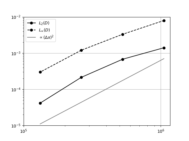
Figure 4: Flow over a mountain test case: normalised depth errors at day 15 versus average mesh size $\Delta x$.

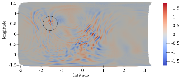
Figure 5: Flow over a mountain test case: depth errors (in metres) at day 15. The range is min:$-1.74\text{m}$, max: $1.78\text{m}$.

Up until this point the flow is only weakly nonlinear (see Figure 7) so, as in Thuburn et al. (2013), we continued the highest resolution simulation until day 50. By this time, fine scale structure has been generated as the flow becomes more nonlinear; the PV field develops sharp gradients and filaments that stretch out and roll up. These features can be seen in the potential vorticity field at 50 days, shown in Figure 7.

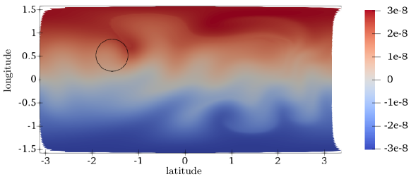
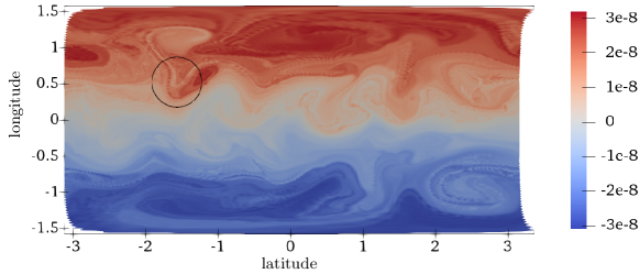
Figure 6: Flow over a mountain test case: potential vorticity at day 15. The range is min:$-3.05\times 10^{-8}(\text{ms})^{-1}$, max: $3.05\times 10^{-8}(\text{ms})^{-1}$. The circle indicates the position of the mountain.

Figure 7: Flow over a mountain test case: potential vorticity at day 50. The range is min:$-3.1\times 10^{-8}(\text{ms})^{-1}$, max: $3.2\times 10^{-8}(\text{ms})^{-1}$. The circle indicates the position of the mountain.

3.3 Barotropically unstable jet (Galewsky)

The details of this test case are specified in Galewsky et al. (2004). The initial condition consists of a strong midlatitude jet, with an added perturbation, which is barotropically unstable and evolves to produce vortices and small scale structure. It has become a particularly useful test for models on grids that are not aligned with latitude/longitude because these grids can induce early development of the instability and even lead to the final solution (at day 6) having the incorrect wavenumber. Again, there is no analytic solution so results are compared to those in the literature (see for example Thuburn et al. (2013) and Weller (2013)). An important feature to reproduce is the relatively straight path of the jet across approximately quarter of the globe - this is not seen in models where grid imprinting has resulted in the generation of instability along the length of the jet (Weller, 2013).

Figure 8 shows the vorticity field, computed on the highest resolution grid (see table 1) with timestep of $120\text{s}$, in the Northern hemisphere after 6 days. The maximum Courant number reached during this simulation is $0.28$. We note that the jet has the correct wavenumber and the expected quiescent section. Lower resolution simulations, as others have found (Thuburn et al., 2013), did not have these requisite features. The conservation properties of the algorithm are demonstrated in table 4 which gives values of the normalised integral of the potential vorticity over the sphere,

$$Q=\frac{\int_{\Omega}qD\operatorname{d\!}V}{\|q_{0}\|_{L^{2}}\|D_{0}\|_{L^{2}}}$$ (78)

where $q_{0}$ and $D_{0}$ are the initial values of the potential vorticity and depth respectively, and $\|\cdot\|_{L^{2}}$ indicates the (un-normalised) $L^{2}$ norm. This is conserved (and zero) by construction (see equation 19 and the following discussion).

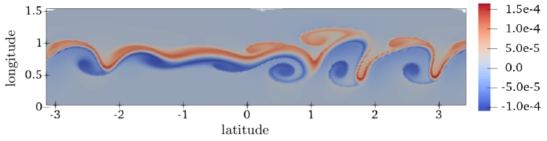
Figure 8: Snapshot of the northern hemisphere relative vorticity field at day 6 for the Galewsky jet test. The range is min: $-1.10\times 10^{-4}(\text{ms})^{-1}$, max: $1.66\times 10^{-4}(\text{ms})^{-1}$.

Time (days)	$Q$		$Q$
0	$-5.70\text{\times}{10}^{-15}$	Min:	$-1.80\text{\times}{10}^{-14}$
2	$-5.22\text{\times}{10}^{-15}$	Max:	$1.73\text{\times}{10}^{-14}$
4	$1.05\text{\times}{10}^{-14}$	Mean:	$4.23\text{\times}{10}^{-16}$
6	$-2.02\text{\times}{10}^{-16}$	Standard deviation:	$4.36\text{\times}{10}^{-15}$

Table 4: Values of $Q$ (see equation 78) for the Galewsky test case.

4 Summary and Outlook

We have built upon the work of Cotter and Shipton (2012) and McRae and Cotter (2014) to produce a semi-implicit compatible finite element model for the nonlinear rotating shallow water equations on the sphere. The important features are that we introduce higher-order upwind advection schemes that maintain PV conservation, and consistency of PV advection with the mass conservation law. By applying the model to standard test cases we have demonstrated that this model has the expected second order convergence rate and can produce the required features of both large scale balanced flows and unstable turbulent flows. The developments of this paper inform our ongoing development of a three dimensional dynamical core on the sphere.

Acknowledgements

The authors would like to thank John Thuburn for providing the semi-Lagrangian code that was used for the Williamson 5 convergence test, and the Firedrake project (Rathgeber et al., 2016; Luporini et al., 2016; Homolya et al., 2017; Kirby and Mitchell, 2017; Gibson et al., 2018), along with PETSc (Balay et al., 2016, 1997) and other upstream tools (Hendrickson and Leland, 1995; Dalcin et al., 2011) for making the code development in this paper possible. This research was conducted with support from Natural Environment Research Council grants NE/I000747/1 and NE/K006789/1.

References

- Alnæs et al. [2014] Martin S. Alnæs, Anders Logg, Kristian B. Ølgaard, Marie E. Rognes, and Garth N. Wells. Unified form language: A domain-specific language for weak formulations of partial differential equations. ACM Transactions on Mathematical Software (TOMS), 40(2):9, 2014.
- Arakawa and Lamb [1981] Akio Arakawa and Vivian R. Lamb. A potential enstrophy and energy conserving scheme for the shallow water equations. Monthly Weather Review, 109(1):18–36, 1981.
- Arnold et al. [2006] DN Arnold, RS Falk, and R Winther. Finite element exterior calculus, homological techniques, and applications. Acta Numerica, 15(1):1–155, 2006.
- Arnold et al. [2014] DN Arnold, D Boffi, and F Bonizzoni. Finite element differential forms on curvilinear cubic meshes and their approximation properties. Numer. Math., 2014. doi: 10.1007/s00211-014-0631-3. arXiv:1204.2595.
- Balay et al. [1997] Satish Balay, William D. Gropp, Lois Curfman McInnes, and Barry F. Smith. Efficient management of parallelism in object oriented numerical software libraries. In E. Arge, A. M. Bruaset, and H. P. Langtangen, editors, Modern Software Tools in Scientific Computing, pages 163–202. Birkhäuser Press, 1997.
- Balay et al. [2016] Satish Balay, Shrirang Abhyankar, Mark F. Adams, Jed Brown, Peter Brune, Kris Buschelman, Lisandro Dalcin, Victor Eijkhout, William D. Gropp, Dinesh Kaushik, Matthew G. Knepley, Lois Curfman McInnes, Karl Rupp, Barry F. Smith, Stefano Zampini, Hong Zhang, and Hong Zhang. PETSc users manual. Technical Report ANL-95/11 - Revision 3.7, Argonne National Laboratory, 2016.
- Bochev and Ridzal [2008] PB Bochev and D Ridzal. Rehabilitation of the lowest-order Raviart-Thomas element on quadrilateral grids. SIAM Journal on Numerical Analysis, 47(1):487–507, 2008.
- Boffi and Gastaldi [2009] D Boffi and L Gastaldi. Some remarks on quadrilateral mixed finite elements. Computers & Structures, 87(11):751–757, 2009.
- Boffi et al. [2013] D Boffi, F Brezzi, and M Fortin. Mixed finite element methods and applications. Springer, 2013.
- Brooks and Hughes [1982] Alexander N Brooks and Thomas JR Hughes. Streamline upwind/Petrov-Galerkin formulations for convection dominated flows with particular emphasis on the incompressible Navier-Stokes equations. Computer methods in applied mechanics and engineering, 32(1):199–259, 1982.