Learning Deep Energy Models: Contrastive Divergence vs. Amortized MLE
Abstract
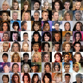
We propose a number of new algorithms for learning deep energy models from data motivated by a recent Stein variational gradient descent (SVGD) algorithm, including a Stein contrastive divergence (SteinCD) that integrates CD with SVGD based on their theoretical connections, and a SteinGAN that trains an auxiliary generator to generate the negative samples in maximum likelihood estimation (MLE). We demonstrate that our SteinCD trains models with good generalization (high test likelihood), while SteinGAN can generate realistic looking images competitive with GAN-style methods. We show that by combing SteinCD and SteinGAN, it is possible to inherent the advantage of both approaches.
1 Introduction
Energy-based models (EBMs) capture dependencies between variables by associating a scalar energy to each configuration of the variables. Learning EBMs consists in finding an energy function that assigns low energy to correct values, and high energy to incorrect values. Energy-based learning provides a unified framework for many learning models, such as undirected graphical models (LeCun et al., 2006), deep generative models (Ngiam et al., 2011; Xie et al., 2016).
Maximum likelihood estimator (MLE) provides a fundamental approach for learning energy-based probabilistic models from data. Unfortunately, exact MLE is intractable to calculate due to the difficulty of evaluating the normalization constant and its gradient. This problem has attracted a vast literature in the last few decades, based on either approximating the likelihood objective, or developing alternative surrogate loss functions (see e.g., Koller & Friedman, 2009; Goodfellow et al., 2016, for reviews). Contrastive divergence (CD) (Hinton, 2002) is one of the most important algorithms, which avoids estimating the normalization constant by optimizing a contrastive objective that measures how much KL divergence can be improved by running a small numbers of Markov chain steps towards the intractable energy model. CD has been widely used for learning models like restricted Boltzmann machines and Markov random fields (Carreira-Perpinan & Hinton, 2005; Hinton & Salakhutdinov, 2006).
Although being able to train models that have high testing likelihood, CD and other traditional energy-based learning algorithms can not generate high quality samples that resemble real-world instances, such as realistic-looking images. This is because the real world instances live a relatively low manifold which the the energy-based models can not capture. This problem has been addressed by the recent generative adversarial networks (GAN) (e.g., Goodfellow et al., 2014; Radford et al., 2015; Salimans et al., 2016; Arjovsky et al., 2017, to name only a few), which, instead of training energy models, directly train generative networks that output random samples to match the observed data by framing the divergence minimization problem into a minimax game. By designing the generator using deep convolutional networks (Radford et al., 2015), the prior knowledge of the real-world manifold can be incorporated into learning. However, GAN does not explicitly assign an energy score for each data point, and can over-fit on a subset of the training data, and ignore the remaining ones. A promising direction is to combine GAN-type methods with traditional energy-based learning to integrate the advantages of both.
Based on a recent Stein variational gradient descent (SVGD) algorithm for approximate inference (Liu & Wang, 2016), we propose a number of new algorithms for training deep energy models, including a Stein contrastive divergence (SteinCD) that combines CD with SVGD based on their theoretical connections, and a SteinGAN algorithm that approximates MLE using a sampler (generator) that amortizes the negative sample approximation. We show that SteinCD and SteinGAN exhibit opposite properties, SteinCD tends to learn models with high testing likelihood but can not generate high quality images, while SteinGAN generates realistic looking images but does not generalize well. Our SteinGAN approach suggests that it is possible to generate high quality images comparable with GAN-type methods using energy-based models, opening the possibility of combining the traditional energy-based learning techniques with GAN approaches. In experiments, we show evidence that by simply mixing SteinCD and SteinGAN updates it is possible to obtain algorithms that combine the advantage of both.
Outline
2 Background
In this section, we first introduce the background of Stein variational gradient descent (SVGD) which forms the foundation of our work, and then review energy-based probabilistic models and contrastive divergence (CD). Our introduction highlights the connection between SVGD and CD which motivates us to propose SteinCD in Section 3.
2.1 Stein Variational Gradient Descent (SVGD)
Stein variational gradient descent (SVGD) (Liu & Wang, 2016) is a general purpose deterministic approximate sampling method. The idea is to iteratively evolve a set of particles to yield the fastest decrease of KL divergence locally.
Let be a positive density function in that we want to approximate. Assume we start with a set of particles whose empirical distribution is , and want to move closer to the target distribution to improve the approximation quality. To do so, assume we update the particles by a transform of form
where is a small step size and is a velocity field that decides the perturbation direction of the particles. Ideally, should be chosen to maximally decrease the KL divergence with ; this can be framed as the following optimization problem:
| (1) |
where is the (empirical) distribution of when , and is a predefined function space that we optimize over. Note that although can be infinite (or illy defined) when is an empirical delta measure, the difference of KL divergence in Eq. (1) can be finite because the infinite parts cancel out with each other. This can be checked by first approximating by a Gaussian mixture with variance , and then show that the limit exists and is finite when taking to zero.
Equation (1) defines a challenging nonlinear functional optimization problem. It can be simplified by assuming the step size , in which case the decreasing rate of KL divergence can be approximated by the gradient of the KL divergence w.r.t. at , that is,
| (2) |
Further, Liu & Wang (2016) showed that the gradient objective in (2) can be expressed as a linear functional of ,
where is a linear operator acting on a vector-valued function and returns a scalar-valued function, and is called the Stein operator in connection with the so called Stein’s identity, which says that when as a result of integration by parts.
Therefore, the optimization in (2) reduces to
| (3) |
where provides a notation of discrepancy measure between and and is known as the Stein discrepancy. If is taken to be rich enough, only if there exists no velocity field that can decrease the KL divergence between and , which must imply .
The problem can be further simplified by taking a set to have “simple” structures, but still remain to be infinite dimensional to catch all the possible useful velocity fields. A natural choice, motivated by kernel methods (e.g., Scholkopf & Smola, 2001), is to take to be the unit ball of a vector-valued reproducing kernel Hilbert space (RKHS) , where each is a scalar-valued RKHS associated with a positive definite kernel , that is,
Briefly speaking, is the closure of functions of form , , , equipped with norm . With this choice, Liu et al. (2016) showed the optimal solution of (3) is , where
| (4) |
where denotes the outer product version of Stein operator, which acts on a scalar-valued function and outputs a vector-valued function (velocity field).
Therefore, provides the best update direction within RKHS . By repeatedly applying this update starting with a set of initial particles, we obtain the SVGD algorithm:
| (5) | ||||
Update (5) mimics a gradient dynamics at the particle level, where the two terms in play different roles: the term with the gradient drives the particles toward the high probability regions of , while the term with serves as a repulsive force to encourage diversity as shown in Liu & Wang (2016).
It is easy to see from (5) that reduces to the typical gradient when there is only a single particle () and when , in which cases SVGD reduces to the standard gradient ascent for maximizing (i.e., maximum a posteriori (MAP)).
2.2 Learning Energy Models
SVGD is an inference process in which we want to find a set of particles (or “data”) to approximate a given distribution . The goal of this paper is to investigate the learning problem, the opposite of inference, in which we are given a set of observed data and we want to construct a distribution , found in a predefined distribution family, to best approximate the data.
In particular, we assume the observed data is i.i.d. drawn from an unknown distribution indexed by a parameter , of form
| (6) | ||||
where is a scalar-valued function that represents the negative energy of the distribution, and is the partition function which normalizes the distribution. A fundamental approach for estimating is the maximum likelihood estimation (MLE):
| (7) |
where is the log-likelihood function. For the energy-based model in (6), the gradient of can be shown to be
| (8) |
where we still use to denote the empirical distribution of data . This gives a gradient ascent update for solving MLE:
where is the step size. Intuitively, this update rule iteratively decreases the energy of the observed data (or the positive samples), while increases the energy of the negative samples, drawn from the hypothesized model . When the algorithm converges, we should have , which is a moment matching condition between the empirical and the model-based averages of .
However, critical computational challenges arise, because it is intractable to exactly calculate the model-based expectation and efficient approximation is needed. One way is to use Markov chain Monte Carlo (MCMC) to approximate the expectation (e.g., Geyer, 1991; Snijders, 2002). Unfortunately, MCMC-MLE is often too slow in practice, given that we need to approximate the expectation repeatedly at each gradient update step.
Contrastive Divergence
Maximum likelihood estimation can be viewed as finding the optimal to minimize the KL divergence between the empirical data distribution and the assumed model :
| (9) |
Contrastive divergence (Hinton, 2002) is an alternative method that optimizes a different objective function:
| (10) |
where is a distribution obtained by moving towards for k steps, more precisely, by running steps of Markov transitions whose equilibrium distribution , starting from the empirical distribution . is always non-negative because running Markov chain forward can only decrease the KL divergence (Cover & Thomas, 2012), and equals zero only if matches . Observe that Eq. (10) and (1) share a similar objective function, but optimize different variables ( vs. ). Their similarity is the main motivation of our Stein contrastive divergence algorithm (Section 3).
Taking gradient descent on the objective (without differentiating through ) gives the following update rule:
| (11) |
Compared with the MLE update (8), the CD- update replaces the “ideal” negative sample drawn from with a local -step perturbation of the observed data. Although CD- can be viewed as MLE, the key observation of Hinton (2002) is that even by using a small , such as , we obtain useful contrastive information about how the parameter should be improved.
3 Stein Contrastive Divergence
The performance of CD depends on the choice of Markov chain it uses; it is clear that we should select the Markov chain to minimize and hence maximize the contrastive objective (10), bringing it closer to the MLE objective (9). However, it is unclear how to frame the optimal choice of Markov chains into an solvable optimization problem. SVGD provides a natural solution for this, given that it explicitly provides the best perturbation direction that maximizes the very same contrastive objective.
To be more specific, assume we perturb the observed data with a deterministic transform as in SVGD, where the velocity field is decided jointly with the model parameter by solving the following minimax problem:
| (12) |
We then solve this problem by alternating between minimizing and maximizing . Following the derivation of SVGD, with small step size , has a closed form solution shown in (4), and the gradient update of is
| (13) |
where we update using the result of one step of SVGD update on the observed data as the negative samples. This gives our Stein contrastive divergence shown in Algorithm 1, which replaces the -step Markov chain perturbation in typical CD with a SVGD update.
Stein Score Matching
We should keep the step size small to make the derivation valid. If we explicitly take , then the minimax problem in (12) reduces to minimizing the Stein discrepancy between the data distribution and model , that is,
| (14) |
which is the result of Eq. (2) and (3). From this perspective, it is possible to take (14) and directly derive a gradient descent algorithm for minimizing the Stein discrepancy (14). From , we can derive that
where is the -valued cross derivative of where and are the dimensions of and , respectively. This gives the following update:
| (15) |
We call this update rule Stein score matching in connection with the score matching algorithm (Hyvärinen, 2005) which minimizes Fisher divergence.
In practice, it can be cumbersome to calculate the cross derivative . It turns out the SteinCD update (13) can be viewed as approximating in (15) with a finite difference approximation:
| (16) |
Alternatively, it is also possible to use a symmetric finite difference formula:
This corresponds to
| (17) |
which perturbs the data on both opposite directions and uses the difference to guild the update of .
In practice, we prefer the original update (13) because of its simplicity. Note that unlike SVGD, there is no cost in using a small step size beyond the error caused by numerical rounding, since we just need to obtain a correct moving direction, do not need to actually move the particles (the observed data) to . Therefore, we can use a relatively small , in which case (13), (15) and (17) are all close to each other.
It is worth comparing Stein score matching (15) with the (Fisher) score matching (Hyvärinen, 2005), which estimates by minimizing the Fisher divergence:
| (18) |
Fisher divergence is a stronger divergence measure than Stein discrepancy, which equals infinite (like KL divergence) if is an empirical delta measure, because does not exist for delta measures. In contrast, Stein discrepancy remains to be finite for empirical measure because it depends on only through the empirical averaging .
Nevertheless, like the case of KL divergence, the infinite part of Fisher divergence does not depend on , and it is still possible to minimize (18) as shown in Hyvärinen (2005), by using integration by parts. The main disadvantage of Fisher score matching is that it has a relatively complex formula, and involves calculating a third order derivative that makes it difficult to implement. In contrast, SteinCD only involves calculating the first order derivatives and is straightforward to implement.
4 Amortized MLE
CD-type algorithms have been widely used for learning energy-based models, and can often train models with good test likelihood. However, models trained by CD can not generate realistic looking images (when is used to model image pixels). This is because CD learns the models based on a local perturbation in the neighborhood of the observed data, and does not explicitly train the model to create images from scratch. This problem has been addressed recently by generative adversarial networks (GAN) (Goodfellow et al., 2014; Radford et al., 2015), which explicitly train a generator, a deep neural network that takes random noise and outputs images, to match the observed data with the help of a discriminator that acts adversarially, to distinguish the generated data from the observed ones. Motivated by GAN, we modify the MLE and CD idea to explicitly incorporate a generator into the training process.
Our idea is based on “amortizing” the sampling process of with a generator and use the simulated samples as the negative samples to update . To be specific, let be a neural network that takes a random noise as input and outputs a sample , with a parameter which we shall adjust adaptively to make the distribution of approximates the model , and we update by
| (19) |
where denotes the average on random variable The key question here is how to update so that the distribution of closely approximates the target distribution . This problem is addressed by a recent amortized SVGD algorithm (Wang & Liu, 2016), as we introduce as follows.
Amortized SVGD
The idea of amortized SVGD is to leverage the Stein variational gradient direction (2) to guid the update of the generator , in order to match its output distribution with . To be specific, at each iteration of amortized SVGD, we generate a batch of random outputs where , based on the current parameter . The Stein variational gradient in (5) would then ensure that forms a better approximation of the target distribution . Therefore, we should adjust to make the output of the generator match the updated points . This can be done by updating via
| (20) |
Essentially, this projects the non-parametric perturbation direction to the change of the finite dimensional network parameter . Assume the step size is taken to be small, so that a single step of gradient descent provides a good approximation of Eq. (20). This gives a simpler update rule:
| (21) |
which can be intuitively interpreted as a form of chain rule that back-propagates the SVGD gradient to the network parameter . In fact, when there is only one particle, (21) reduces to the standard gradient ascent for , in which is trained to “learn to optimize” (e.g., Andrychowicz et al., 2016), instead of “learn to sample” . Importantly, as there are more than one particles, the repulsive term in becomes active, and enforces an amount of diversity on the network output that is consistent with the variation in .
Amortized MLE
Updating and alternatively with (19) and (20) or (21) allows us to simultaneously train an energy model together with a generator (sampler). This approach is presented as Algorithm 2. Compared with the traditional methods based on MCMC-MLE or contrastive divergence, we amortize the sampler as we train, which saves computation in long term and simultaneously provides a high quality generative neural network that can generate realistic-looking images.
Formally, our method can be viewed as approximately solving the following minimax objective function based on KL divergence:
| (22) |
where denotes the distribution of the output of the generator . Here the energy model , serving as a discriminator, attempts to get closer to the observed data , and keep away from the “fake” data distribution , both in terms of KL divergence, while the generator attempts to get closer to the energy model using amortized SVGD. We call our method SteinGAN to reflect this interpretation. It can be viewed as a KL-divergence variant of the GAN-style adversarial game (Goodfellow et al., 2014).
| (23) |
Related Work
The idea of training energy models with neural samplers was also discussed by Kim & Bengio (2016); Zhai et al. (2016); one of the key differences is that the neural samplers in Kim & Bengio (2016); Zhai et al. (2016) are trained with the help of heuristic diversity regularizers, while SVGD enforces the diversity in a more principled way. Another method by Zhao et al. (2016) also trains an energy function to distinguish real and simulated samples, but within a non-probabilistic framework.
Generative adversarial network (GAN) and its variants have recently gained remarkable success in generating realistic-looking images (Goodfellow et al., 2014; Salimans et al., 2016; Radford et al., 2015; Li et al., 2015; Dziugaite et al., 2015; Nowozin et al., 2016; Arjovsky et al., 2017, to name a few). All these methods are set up to train implicit models specified by the generators, and are different from the energy model assumption. The main motivation of SteinGAN is to show the possibility of obtaining comparable image generation results using energy-based learning, allowing us to combine the advantages of these two types of approaches.
test data log likelihood
|
inception score
 test data log likelihood
|
|
 |
| (a) Iterations () | (b) CD update ratio () | (c) SteinGAN | (d) SteinGAN w/o kernel |
5 Experiments
We evaluated SteinCD and SteinGAN on four datasets, including MNIST, CIFAR-10, CelebA (Liu et al., 2015), and Large-scale Scene Understanding (LSUN) (Yu et al., 2015). We observe: 1) SteinCD tends to outperform typical CD equipped with Langevin dynamics; 2) SteinCD tends to provide better test likelihood than SteinGAN, while SteinGAN generates better images; 3) by interleaving SteinCD and SteinGAN updates, it is possible to combine advantages of both, obtaining both good testing likelihood and images. We will provide code to reproduce our experiments.
5.1 Restricted Boltzmann Machine on MNIST
In this section, we evaluate our methods on MNIST and use a simple Gaussian-Bernoulli Restricted Boltzmann Machines (RBM) as our energy-based model, which allows us to accurately evaluate the test likelihood. Gaussian-Bernoulli RBM is a hidden variable model of form
where is a continuous observed variable and is a binary hidden variable; is the normalization constant. By marginalizing out the hidden variable , we obtain with negative energy
where . To evaluate the test likelihood exactly, we use a small model with only hidden units which allows us to calculate using exact variable elimination. We use mini-batches of size 100 and Adam (Kingma & Ba, 2014) for our gradient updates. Following Liu & Wang (2016), we use a RBF kernel in SVGD, with the bandwidth selected to be ( is the median of the pairwise distance of and is the minibatch size). For SteinGAN, the generator consists of 2 fully connected layers, followed by 2 deconvolution layers with filters.
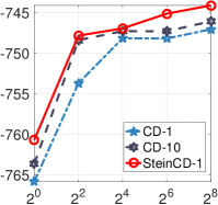
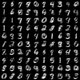
Figure 1(a) shows the test likelihood of the CD-type methods, where we can find that SteinCD (with a single step of SVGD) outperforms both CD-1 and CD-10 equipped with Langevin dynamics. We also evaluated the test likelihood of SteinGAN but find it gives worse test likelihood (not shown in the figure). The advantage of SteinGAN, however, is that it trains a generator that produces high quality and diverse images (Figure 1(c)), which SteinCD can not generate (even when we train another generator on the energy model obtained by SteinCD, which has better test likelihood).
Mixing SteinCD and SteinGAN
It seems that SteinCD and SteinGAN have opposite properties in terms of test likelihood and image quality. This motivates us to integrate SteinCD and SteinGAN to combine their advantages. In order to do this, we replace the neural-simulated sample (step 4 in Algorithm 2) with the SVGD-updated sample in SteinCD (step 2 of Algorithm 1) with a probability . We use SteinCD-GAN() to denote this algorithm, which reduces to SteinCD with and SteinGAN with .
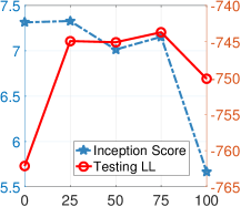
The performance of SteinCD-GAN() with different -values is shown in Figure 1(b), where we find that mixing even a small percentage of CD-updates (e.g., ) can significantly improve the test likelihood, even slightly higher than the pure SteinCD algorithm.
We also evaluate the inception score of the images generated by SteinCD-GAN(), using an inception model trained on the MNIST training set (result averaged on 50,000 generated images). As shown in Figure 1(b), we find that adding CD updates seems to deteriorate the image quality, but only slightly unless we use CD updates (). Overall, Figure 1(b) suggests that by mixing SteinGAN with a small percentage of CD updates (e.g., ), we obtain results that perform well both in terms of test likelihood and image quality.
Effect of the Repulsive Force
As it is discussed in Section 2.1, the repulsive term in SVGD (5) enforces the particles to be different from each other and produces an amount of variability required for generating samples from . In order to investigate the effect of the repulsive term . We test a variant of SteinGAN in which the Stein variational gradient is replaced by the typical gradient (or, effectively, use a constant kernel in )); this corresponds to an amortized variant of Viterbi learning (Koller & Friedman, 2009), or Herding algorithm (Welling, 2009) that maximizes as the learning objective function.
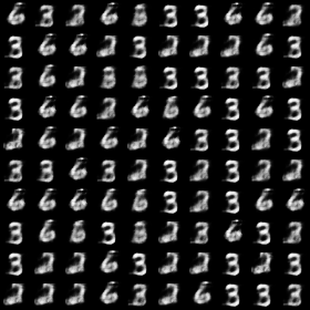
As shown in Figure 1(d), SteinGAN without the kernel tends to produce much less diverse images. This suggests that the repulsive term is responsible for generating diverse images in SteinGAN.
| airplane automobile bird cat deer dog frog horse ship truck |
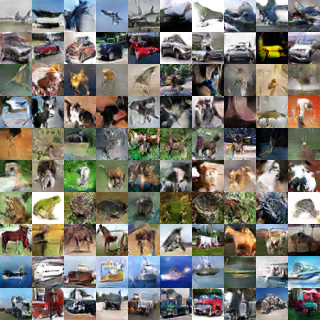
|
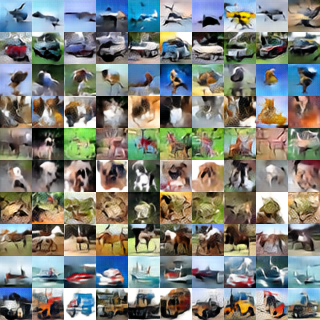 |
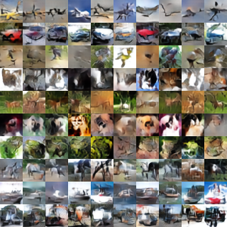 |
|---|---|---|---|
| DCGAN | SteinGAN | SteinGAN w/o kernel |
| Real Training Set | 500 Duplicate | DCGAN | SteinGAN | SteinGAN w/o kernel | |
|---|---|---|---|---|---|
| Inception Score | 11.237 | 11.100 | 6.581 | 6.711 | 6.243 |
| Testing Accuracy | 92.58 % | 44.96 % | 44.78 % | 61.09 % | 60.50 % |
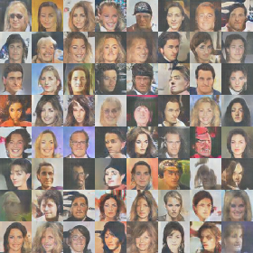 |
 |
| DCGAN | SteinGAN |
 |
 |
 |
| DCGAN | SteinGAN |
5.2 Deep Autoencoder-based SteinGAN
In order to obtain better results on realistic datasets, we test a more complex energy model based on deep autoencoder:
| (24) |
where denotes the image and , is a pair of encoder/decoder function, indexed by parameter . This choice is motivated by Energy-based GAN (Zhao et al., 2016) in which the autoencoder is used as a discriminator but without a probabilistic interpretation. We assume to be a neural network whose input is a -dimensional random vector drawn by . Leveraging the latent representation of the autoencoder, we find it useful to define the kernel on the encoder function, that is, We take the bandwidth to be , where is the median of the pairwise distances between on the image simulated by . This makes the kernel change adaptively based on both (through ) and (through bandwidth ). Note that the theory of SVGD does not put constraints on the choice of positive definite kernels, and it allows us to obtain better results by changing the kernel adaptively during the algorithm.
Some datasets include both images and their associated discrete labels . In these cases, we train a joint energy model on to capture both the inner structure of the images and its predictive relation with the label, which allows us to simulate images with a control on the category which it belongs to. Our joint energy model is defined by
| (25) |
where is the cross entropy loss function of a fully connected output layer. In this case, our neural sampler first draws a label randomly according to the empirical counts in the dataset, and then passes into a neural network together with a random vector to generate image . This allows us to generate images for particular categories by controlling the value of input .
We compare our algorithm with DCGAN. We use the same generator architecture as DCGAN. To be fair, our energy model has comparable or less parameters than the discriminator in the DCGAN. The number of parameters used are summarized in Table 1.
Stabilization
In practice, we find it is useful to modify (23) in Algorithm 2 to be
where is a discount factor (which we take to be ). This is equivalent to maximizing a regularized likelihood:
where is the log-partition function (see (6)); note that is a conjugate prior of .
We initialize the weights of both the generator and discriminator from Gaussian distribution , and train them using Adam (Kingma & Ba, 2014) with a learning rate of for the generator and for the energy model (the discriminator). To keep the generator and discriminator approximately aligned during training, we speed up the -update (by increasing the discount factor to ) when the energy of the real data batch is larger than the energy of the simulated images. We used the architecture guidelines for stable training suggested in DCGAN (Radford et al., 2015).
| Cifar10 | CelebA & LSUN | |
|---|---|---|
| DCGAN | ||
| SteinGAN |
Discussion
CIFAR-10 includes diverse objects, but has only 50,000 training examples. Figure 2 shows examples of simulated images by DCGAN and SteinGAN generated conditional on each category, which look equally well visually. It is still an open question on how to quantitively evaluate the quantities of simulated images. In order to gain some understanding, here we report two different scores, including the inception score proposed by Salimans et al. (2016), and the classification accuracy when training ResNet using simulated images as train sets, evaluated on a separate held-out testing set never seen by the GAN models. Besides DCGAN and SteinGAN, we also evaluate another simple baseline obtained by subsampling 500 real images from the training set and duplicating them 100 times. We observe that these scores capture rather different perspectives of image generation: the inception score favors images that look realistic individually and have uniformly distributed labels; as a result, the inception score of the duplicated 500 images is almost as high as the real training set. We find that the inception score of SteinGAN is comparable with DCGAN. On the other hand, the classification accuracy measures the amount information (in terms of classification using ResNet) captured in the simulated image sets; we find that SteinGAN achieves higher classification accuracy, suggesting that it captures, at least in some perspective, more information in the training set.
6 Conclusion
We propose a number of new algorithms for learning deep energy models, and demonstrate their properties. We show that our SteinCD performs well in term of test likelihood, while SteinGAN performs well in terms of generating realistic looking images. Our results suggest promising directions for learning better models by combining GAN-style methods with traditional energy-based learning.
References
- Andrychowicz et al. (2016) Andrychowicz, Marcin, Denil, Misha, Gomez, Sergio, Hoffman, Matthew W, Pfau, David, Schaul, Tom, and de Freitas, Nando. Learning to learn by gradient descent by gradient descent. arXiv preprint arXiv:1606.04474, 2016.
- Arjovsky et al. (2017) Arjovsky, Martin, Chintala, Soumith, and Bottou, Léon. Wasserstein gan. arXiv preprint arXiv:1701.07875, 2017.
- Carreira-Perpinan & Hinton (2005) Carreira-Perpinan, Miguel A and Hinton, Geoffrey E. On contrastive divergence learning. In AISTATS, volume 10, pp. 33–40. Citeseer, 2005.
- Cover & Thomas (2012) Cover, Thomas M and Thomas, Joy A. Elements of information theory. John Wiley & Sons, 2012.
- Dziugaite et al. (2015) Dziugaite, Gintare Karolina, Roy, Daniel M., and Ghahramani, Zoubin. Training generative neural networks via maximum mean discrepancy optimization. In Conference on Uncertainty in Artificial Intelligence (UAI), 2015.
- Geyer (1991) Geyer, Charles J. Markov chain monte carlo maximum likelihood. 1991.
- Goodfellow et al. (2014) Goodfellow, Ian, Pouget-Abadie, Jean, Mirza, Mehdi, Xu, Bing, Warde-Farley, David, Ozair, Sherjil, Courville, Aaron, and Bengio, Yoshua. Generative adversarial nets. In Advances in Neural Information Processing Systems, pp. 2672–2680, 2014.
- Goodfellow et al. (2016) Goodfellow, Ian, Bengio, Yoshua, and Courville, Aaron. Deep learning. MIT Press, 2016.
- He et al. (2016) He, Kaiming, Zhang, Xiangyu, Ren, Shaoqing, and Sun, Jian. Deep residual learning for image recognition. In Proceedings of the IEEE Conference on Computer Vision and Pattern Recognition, pp. 770–778, 2016.
- Hinton (2002) Hinton, Geoffrey E. Training products of experts by minimizing contrastive divergence. Neural computation, 14(8):1771–1800, 2002.
- Hinton & Salakhutdinov (2006) Hinton, Geoffrey E and Salakhutdinov, Ruslan R. Reducing the dimensionality of data with neural networks. science, 313(5786):504–507, 2006.
- Hyvärinen (2005) Hyvärinen, Aapo. Estimation of non-normalized statistical models by score matching. In Journal of Machine Learning Research, pp. 695–709, 2005.
- Kim & Bengio (2016) Kim, Taesup and Bengio, Yoshua. Deep directed generative models with energy-based probability estimation. arXiv preprint arXiv:1606.03439, 2016.
- Kingma & Ba (2014) Kingma, Diederik and Ba, Jimmy. Adam: A method for stochastic optimization. arXiv preprint arXiv:1412.6980, 2014.
- Koller & Friedman (2009) Koller, Daphne and Friedman, Nir. Probabilistic graphical models: principles and techniques. MIT press, 2009.
- LeCun et al. (2006) LeCun, Yann, Chopra, Sumit, Hadsell, Raia, Ranzato, M, and Huang, F. A tutorial on energy-based learning. Predicting structured data, 1:0, 2006.
- Li et al. (2015) Li, Yujia, Swersky, Kevin, and Zemel, Richard. Generative moment matching networks. In International Conference on Machine Learning, pp. 1718–1727, 2015.
- Liu & Wang (2016) Liu, Qiang and Wang, Dilin. Stein variational gradient descent: A general purpose bayesian inference algorithm. In Advances In Neural Information Processing Systems, pp. 2370–2378, 2016.
- Liu et al. (2016) Liu, Qiang, Lee, Jason D, and Jordan, Michael I. A kernelized Stein discrepancy for goodness-of-fit tests. In Proceedings of the International Conference on Machine Learning (ICML), 2016.
- Liu et al. (2015) Liu, Ziwei, Luo, Ping, Wang, Xiaogang, and Tang, Xiaoou. Deep learning face attributes in the wild. In Proceedings of International Conference on Computer Vision (ICCV), 2015.
- Ngiam et al. (2011) Ngiam, Jiquan, Chen, Zhenghao, Koh, Pang W, and Ng, Andrew Y. Learning deep energy models. In Proceedings of the 28th International Conference on Machine Learning (ICML-11), pp. 1105–1112, 2011.
- Nowozin et al. (2016) Nowozin, Sebastian, Cseke, Botond, and Tomioka, Ryota. f-gan: Training generative neural samplers using variational divergence minimization. arXiv preprint arXiv:1606.00709, 2016.
- Radford et al. (2015) Radford, Alec, Metz, Luke, and Chintala, Soumith. Unsupervised representation learning with deep convolutional generative adversarial networks. arXiv preprint arXiv:1511.06434, 2015.
- Salimans et al. (2016) Salimans, Tim, Goodfellow, Ian, Zaremba, Wojciech, Cheung, Vicki, Radford, Alec, and Chen, Xi. Improved techniques for training gans. In Advances in Neural Information Processing Systems, pp. 2226–2234, 2016.
- Scholkopf & Smola (2001) Scholkopf, Bernhard and Smola, Alexander J. Learning with kernels: support vector machines, regularization, optimization, and beyond. MIT press, 2001.
- Snijders (2002) Snijders, Tom AB. Markov chain monte carlo estimation of exponential random graph models. Journal of Social Structure, 3(2):1–40, 2002.
- Wang & Liu (2016) Wang, Dilin and Liu, Qiang. Learning to draw samples: With application to amortized mle for generative adversarial learning. arXiv preprint arXiv:1611.01722, 2016.
- Welling (2009) Welling, Max. Herding dynamical weights to learn. In Proceedings of the 26th Annual International Conference on Machine Learning, pp. 1121–1128. ACM, 2009.
- Xie et al. (2016) Xie, Jianwen, Lu, Yang, Zhu, Song-Chun, and Wu, Ying Nian. A theory of generative convnet. arXiv preprint arXiv:1602.03264, 2016.
- Yu et al. (2015) Yu, Fisher, Seff, Ari, Zhang, Yinda, Song, Shuran, Funkhouser, Thomas, and Xiao, Jianxiong. Lsun: Construction of a large-scale image dataset using deep learning with humans in the loop. arXiv preprint arXiv:1506.03365, 2015.
- Zhai et al. (2016) Zhai, Shuangfei, Cheng, Yu, Feris, Rogerio, and Zhang, Zhongfei. Generative adversarial networks as variational training of energy based models. arXiv preprint arXiv:1611.01799, 2016.
- Zhao et al. (2016) Zhao, Junbo, Mathieu, Michael, and LeCun, Yann. Energy-based generative adversarial network. arXiv preprint arXiv:1609.03126, 2016.