On Dark Matter Interactions with the Standard Model through an Anomalous $Z^{\prime}$

Abstract

We study electroweak scale Dark Matter (DM) whose interactions with baryonic matter are mediated by a heavy anomalous $Z^{\prime}$. We emphasize that when the DM is a Majorana particle, its low-velocity annihilations are dominated by loop suppressed annihilations into the gauge bosons, rather than by p-wave or chirally suppressed annihilations into the SM fermions. Because the $Z^{\prime}$ is anomalous, these kinds of DM models can be realized only as effective field theories (EFTs) with a well-defined cutoff, where heavy spectator fermions restore gauge invariance at high energies. We formulate these EFTs, estimate their cutoff and properly take into account the effect of the Chern-Simons terms one obtains after the spectator fermions are integrated out. We find that, while for light DM collider and direct detection experiments usually provide the strongest bounds, the bounds at higher masses are heavily dominated by indirect detection experiments, due to strong annihilation into $W^{+}W^{-}$, $ZZ$, $Z\gamma$ and possibly into $gg$ and $\gamma\gamma$. We emphasize that these annihilation channels are generically significant because of the structure of the EFT, and therefore these models are prone to strong indirect detection constraints. Even though we focus on selected $Z^{\prime}$ models for illustrative purposes, our setup is completely generic and can be used for analyzing the predictions of any anomalous $Z^{\prime}$-mediated DM model with arbitrary charges.

1 Introduction

While experimental evidence for dark matter (DM) has been well established for decades, the precise nature of DM remains unknown to this day. Searches for non-gravitational interactions of DM use a broad array of techniques to test different models, from tabletop experiments probing axions to ton-scale detectors that are sensitive to DM much heavier than the proton. With many proposed mechanisms for realizing DM in nature, the development of new DM detection methods is a highly active field. Simultaneously, theoretical advances have guided experiment by exploring frameworks that incorporate DM naturally into extensions of the Standard Model (SM).

From a cosmological perspective, thermal freeze-out is one of the simplest ways to account for the observed abundance of DM. The idea that DM is a thermal relic is also attractive phenomenologically, as it implies a connection between the DM relic density and the strength of potential signatures. Now, it is well known that thermal relic DM candidates are subject to strong model-independent constraints, based on unitarity considerations of DM annihilation Griest:1989wd . In particular, a thermal relic DM particle cannot have a mass exceeding $\sim 300$ TeV. In practice, this limit is not easy to saturate and within concrete models the mass bound on a thermal relic is expected to be significantly more modest. While the DM is not necessarily a thermal relic and a plethora of other consistent candidates have been studied in the literature (for reviews see Bertone:2004pz ; Petraki:2013wwa ; Baer:2014eja ), thermal relics are still appealing candidates, both for theoretical reasons and because these bounds tightly constrain their allowed parameter space and in principle allow a thorough study with collider, direct and indirect detection experiments.

Within the thermal freeze-out scenario, it is well known that a particle that interacts weakly and is near the electroweak scale $\sim 1$ TeV would provide approximately the observed DM relic abundance. These so-called weakly interacting massive particles (WIMPs) are still the most popular DM thermal relic candidates, in spite of the fact that large parts of their parameter space have already been ruled out both by direct and indirect detection experiments. Specifically, while the XENON1T experiment provides the strongest direct detection bounds on WIMPs Aprile:2017iyp , indirect limits arise from the observations of Dwarf Spheroidal Galaxies (dSph) by Fermi-LAT Drlica-Wagner:2015xua ; Ackermann:2015zua and of diffuse $\gamma$ rays from the Galactic Center by HESS Abdallah:2016ygi .

In this regard, there is good motivation to consider a broader set of thermal relic candidates, beyond the “standard” WIMP paradigm. This led to the emergence of dark matter effective field theories (EFTs) Goodman:2010yf ; Bai:2010hh ; Goodman:2010ku , which posit higher-dimension operators between DM and SM states. While dark matter EFTs, especially in their non-relativistic formulations Fan:2010gt ; Fitzpatrick:2012ix , are relevant for interpreting the results of direct detection experiments, they are unable to accurately describe the physics of processes where the momentum transfer is comparable to the EFT cut-off scale, as is common in collider searches Busoni:2013lha ; Buchmueller:2013dya ; Busoni:2014sya ; Busoni:2014haa . The requirement to consider ultraviolet completions of dark matter EFTs in these regimes subsequently resulted in the development of simplified DM models. A typical simplified DM model extends the SM by a DM candidate as well as a mediator that communicates between the SM and dark sectors.

Even though it is hard to believe that any simplified model accurately describes all physics beyond the SM, the essential idea is that the key ingredients that determine the experimental signatures related to the DM should be captured correctly by these models. For these purposes simplified models must be able to make proper predictions for the thermal relic abundance, direct detection experiments, neutrino telescopes, $\gamma$ ray telescopes and collider experiments, such as the LHC or a future 100 TeV machine. We will closely investigate this requirement in our work in the context of simplified models with spin-1 mediators.

The idea that the interaction between the SM particles and DM is mediated by a heavy neutral spin-1 boson, that we will further call $Z^{\prime}$, is not new. Refs An:2012va ; Frandsen:2012rk ; Arcadi:2013qia ; Chu:2013jja ; Dudas:2013sia ; Fairbairn:2014aqa ; Lebedev:2014bba ; Alves:2015pea ; Alves:2015mua ; Kahlhoefer:2015bea form merely a partial list of the related contributions. In this particular work we will concentrate on a Majorana fermion DM candidate whose interactions with the SM are mediated by the heavy $Z^{\prime}$, corresponding to a symmetry that appears to be anomalous at the electroweak scale. Anomaly cancellation at high scales is necessary for the overall consistency of the theory, as well as for more practical purposes, most notably the calculation of the couplings of the $Z^{\prime}$ to the SM gauge bosons, which in turn largely determine the DM signatures in indirect detection experiments. This point has been recently emphasized in Jacques:2016dqz . Moreover, many of the $Z^{\prime}$ models employed in describing the results of LHC searches, including the “axial” $Z^{\prime}$ model, are anomalous Boveia:2016mrp ; Albert:2017onk . All such “anomalous” theories must descend from the UV complete ones, where the anomalies are either canceled by spectator fermions Ismail:2016tod , or via the Green-Schwarz mechanism Green:1984sg ; Coriano:2005own; Armillis:2008vp. As has been recently shown in Ref. Ellis:2017tkh , these spectator fermions can be potentially responsible for non-trivial collider signatures and can be more easily accessible at the LHC than the DM itself.

In this paper we will take a different approach. In fact, it is not always necessary to analyze a full UV-complete model to make important predictions for DM signatures in relevant experiments. In particular, we will be especially interested in the anomalous $Z^{\prime}$ couplings to the SM gauge bosons. These couplings determine the annihilation cross sections of DM into SM gauge bosons, affecting the $\gamma$ ray fluxes from dSph and the Galactic Center, as well as signals in neutrino telescopes. To calculate these observables, it is sufficient to consider an EFT with the anomalous $Z^{\prime}$ after the heavy spectators have been integrated out.

In fact, EFTs with low-energy anomalies from integrating out heavy chiral fermions have been considered as early as the 1980s, mostly in the context of the SM without the top quark DHoker:1984mif ; DHoker:1984izu . Indeed the $SU(2)\times U(1)$ electroweak symmetry is anomalous in the absence of the top quark and should be analyzed as an effective field theory with extra degrees of freedom with couplings which compensate for the loss of gauge invariance at the 1-loop level. This approach was further generalized by Preskill in Ref Preskill:1990fr . More recently, the influence of anomalous $Z^{\prime}$ couplings to the SM gauge bosons has been studied in the context of DM Mambrini:2009ad ; Dudas:2009uq ; Dudas:2013sia ; Domingo:2013tna ; Arcadi:2017jqd .

In this work we essentially take the same approach. We formulate “simplified models” of DM with anomalous $Z^{\prime}$ mediators as consistent effective field theories with a cutoff $\Lambda$. We will show, in agreement with the results of Preskill:1990fr , that this cutoff can be much heavier than the mass of the $Z^{\prime}$ and therefore the non-decoupling effects of the heavy spectators can be efficiently captured by the EFT, without explicitly considering these fermionic degrees of freedom. As expected, this EFT uniquely determines the couplings between the heavy $Z^{\prime}$ and the SM gauge bosons in which we will be interested Chu:1996fr; Bilal:2008qx .

Because we are considering an EFT, we will find that some of our amplitudes, including $\chi\chi\to VV$, where $V$ is a SM gauge boson, grow quadratically with energy. This should not be surprising, as the EFT necessarily contains higher dimensional operators, without which gauge invariance is lost. The growth of such amplitudes is tamed at the scale $\Lambda$, where the spectator fermions appear.

In this work we explicitly calculate the annihilation rates of the dark matter into the SM gauge bosons and estimate the bounds, associated with these rates. We choose as examples several anomalous $Z^{\prime}$ models, that illustrate some generic patterns. We emphasize, that while the concrete bounds are always model dependent, the techniques that we illustrate here are completely generic and can be used in any EFT with an anomalous $Z^{\prime}$ mediator.

We find that for DM heavier than $\sim 200$ GeV, these higher dimensional operators dictate that DM annihilation at low velocities is dominated by final states involving gauge bosons. This results in considerable bounds from indirect detection experiments. At larger velocities, such as at DM freeze-out, $p$-wave annihilation into fermions overcomes these operators, which are loop suppressed, and so the DM relic abundance calculation is mostly unaffected by the requirement of anomaly cancellation. We also compare our new indirect detection constraints with direct detection and collider limits. We find that for heavy DM, $\gamma$ ray and neutrino telescopes (depending on the concrete model) provide the strongest bounds on anomalous $Z^{\prime}$ simplified DM models.

The remainder of this paper is organized as follows. In Sec. 2, we describe the effect of integrating out heavy fermions in a consistent theory, yielding an EFT with apparent anomalies at low energy scales. We focus on the induced loop level operators corresponding to these anomalies, and show that the maximum EFT cutoff can be significantly larger than the $Z^{\prime}$ mass. Then in Sec. 3 we specialize to the case of simplified models of DM and motivate a selection of toy models which serve to illustrate the effects of the higher dimensional operators on physical observables. Sec. 4 contains the experimental bounds on these simplified models, paying particular attention to the impact of loop-induced DM annihilation to gauge bosons on indirect detection constraints. We briefly discuss some limitations of our analysis in Sec. 5, including the assumption that the spectator fermions are heavy. Sec. 6 contains our conclusions. Some important numerical results of our calculation are relegated to the Appendix.

2 Low-Energy Effective Theory

In this section we will review building of an EFT for a new gauge group which appears to be anomalous at low energies. We will introduce the new couplings that should necessarily be introduced to restore gauge invariance of the full theory. We will also describe how the couplings between the exotic and SM gauge bosons should be calculated, from anomaly considerations. Throughout we will closely follow the original work by Preskill Preskill:1990fr (as well as slightly more detailed handwritten notes Preskill:1983 ). We also borrow some results from more recent works Anastasopoulos:2008jt ; Racioppi:2009yxa that made practical use of these results in a slightly different context of MSSM augmented with anomalous $Z^{\prime}$s. The reader familiar with this subject may safely skip this section and proceed directly to Sec. 3, where we explain in detail the DM models that we consider, and Sec. 4, where we present our results.

The EFTs that we are describing here can be thought of as descending from fully gauge invariant theories with spontaneously broken gauge symmetry, after some heavy fermions have been integrated out. Given that these fermions are chiral and get masses from gauge symmetry breaking, like the fermions in the SM, the theory below the scale of the heavy fermions appears to be anomalous. In fact, this is exactly what happens in the SM if we integrate out the top quark, as it is the heaviest fermion of the SM D'Hoker:1984ph ; D'Hoker:1984pc . Although the full SM is perfectly anomaly free, as one would expect from a consistent gauge invariant theory, integrating out the top leaves both the hypercharge and the $SU(2)_{L}$ symmetries anomalous, as well as giving rise to the $SU(2)_{L}\times U(1)_{Y}$ mixed anomaly.

The basic procedure of canceling the anomalies in this low energy EFT comes at the price of introducing non-renormalizability. To see this in a working example, let us consider first the $U(1)^{\prime 3}$ triangle in an anomalous Abelian theory. Since the theory is anomalous, gauge invariance is lost and under the $U(1)^{\prime}$ gauge transformation $A_{\mu}\to A_{\mu}+\partial_{\mu}\omega/g^{\prime}$ the effective action transforms as

$$\delta_{\omega}\Gamma=\frac{g^{\prime 2}}{96\pi^{2}}\sum_{i}Q_{i}^{3}\int d^{4}x\,\omega\,\epsilon_{\mu\nu\rho\sigma}F^{\mu\nu}F^{\rho\sigma}~{}.$$ (1)

where $F$ is the field strength associated with $A$. Here $g^{\prime}$ stands for the “gauge” coupling of the $U(1)^{\prime}$ and the sum runs over all the fermions that are charged under the $U(1)^{\prime}$. This transformation simply manifests the fact that in an anomalous theory the gauge invariance is lost. There will also be mixed anomalies between the $U(1)^{\prime}$ and the SM gauge groups, which we consider below.

In our example, the $U(1)^{\prime}$ gauge invariance can be easily restored by introducing a scalar $a$ that transforms under a gauge transformation as $a\to a+v\,\omega$, where $v$ stands for the scale of the $U(1)^{\prime}$ breaking, or, equivalently $v\equiv m_{Z^{\prime}}/g^{\prime}$. Then, the transformation (1) can be restored by introducing the following term:

$${\cal L}=-\frac{g^{\prime 2}}{96\pi^{2}}\sum_{i}Q_{i}^{3}\epsilon_{\mu\nu\rho\sigma}\frac{aF^{\mu\nu}F^{\rho\sigma}}{v}~{}.$$ (2)

Even though (2) appears to cancel the anomaly with a new degree of freedom, this term is merely a Wess-Zumino counterterm that we have added to the action and $a$ is not a genuine degree of freedom. First, it is worth noticing that in spite of the form of Lagrangian term (2), the total Lagrangian is independent of the field $a$ and depends only on its derivative $\partial_{\mu}a$. This fact becomes manifest if we perform a rotation on the fermions $\psi_{i}\to e^{-iQ_{i}a/v}\psi_{i}$. While such a rotation eliminates the term (2), the path integral measure transforms non-trivially under this rotation, inducing a term in the effective action that looks like $\sim\partial_{\mu}a\psi^{\dagger}\bar{\sigma}^{\mu}\psi$.

The kinetic term of the field $a$, which should also be gauge invariant, is of the form

$${\cal L}=\frac{1}{2}\left(\partial_{\mu}a-g^{\prime}vZ^{\prime}_{\mu}\right)^{2}$$ (3)

Even if we start from a theory that does not have this term, it is induced radiatively by the diagrams depicted in Fig. 1, similarly to the Green-Schwarz mechanism.

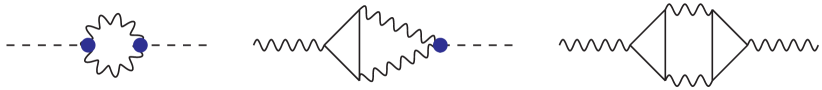
Figure 1: Kinetic term for the field $a$ and the mass term for the $Z^{\prime}$ gauge boson induced by the radiative corrections in the $U(1)$ anomalous theory. Note that each blob corresponds to the couplings (2) and is therefore naturally of the size of the fermionic triangle loop.

This Lagrangian is nothing but a $U(1)$ theory that has been higgsed via a Stückelberg mechanism. In the unitary gauge the scalar degree of freedom $a$ can be set (locally) to zero at any point in space, leaving us simply with an effective theory of the massive gauge bosons with anomalous fermionic field content.

Of course, our effective theory cannot be extrapolated to infinitely high energies, and the calculability requirement sets the cutoff of the theory. In any non-unitary gauge, the presence of the cutoff is evident from the term (2) in the Lagrangian, while in the unitary gauge we can see it from the bad UV behavior of the two-point function of the $Z^{\prime}$. In order to estimate the cutoff of the effective theory, we should remember that loop effects, similar to those that produce the term (3) (see Fig. 1), will also produce terms that look like

$$\sim\frac{1}{(4\pi v)^{p-2}}\frac{1}{v^{p-2}}\left(\partial_{\mu}a-g^{\prime}vZ^{\prime}_{\mu}\right)^{p}$$ (4)

for every power $p\geq 2$. In order to have a consistent EFT, each order in the perturbative expansion (4) should be smaller than its predecessor such that the expansion is valid. Taking this requirement into account (see Preskill:1990fr for the details of this derivation) one finds the following cutoff estimation of the EFT:

$$\Lambda\sim\frac{64\pi^{3}m_{Z}^{\prime}}{\left|g^{\prime}\sum_{i}Q_{i}^{3}\right|}~{}.$$ (5)

Now we can extend this logic to models with more complicated gauge symmetries and mixed anomalies between the $U(1)^{\prime}$ and the non-Abelian gauge groups. This is exactly the situation in which we are interested, where the anomalous $Z^{\prime}$ couples to the DM, and the mixed anomaly will eventually determine the strength of its interaction with the SM gauge bosons.

The treatment of the mixed anomalies will follow a similar logic to one we used in the $U(1)^{\prime}$ case. Let us consider $U(1)^{\prime}\times SU(N)$ symmetry with a mixed anomaly

$$\sum_{i}{\rm Tr}(t^{a}t^{b}Q_{i})={\cal A}\,\delta^{ab}$$ (6)

where $t^{a}$ are the generators of $SU(N)$ The matrix element of this theory between the $Z^{\prime}$ and the $SU(N)$ gauge bosons is nominally divergent, signaling that the theory is non-renormalizable, because there is no tree level coupling between the $Z^{\prime}$ and the $SU(N)$ gauge bosons.

In this case the form of the anomalous transformation is slightly less straightforward to derive. However, it can be obtained by invoking the Wess-Zumino consistency condition Wess:1971yu . Under $U(1)^{\prime}$ and $SU(N)$ transformations with transformation parameters $\omega_{1}$ and $\omega_{N}$, respectively, the action transforms as:

$$\delta_{\omega_{1}}\Gamma = C_{1}\frac{g_{N}^{2}}{16\pi^{2}}{\cal A}\operatorname{Tr}\int d^{4}x\omega_{1}\left(F_{N}^{\mu\nu}\tilde{F}_{N\mu\nu}\right)$$ (7)

$$\delta_{\omega_{N}}\Gamma = C_{N}\frac{g^{\prime}_{1}g_{N}}{8\pi^{2}}{\cal A}\int d^{4}x\tilde{F}_{1}^{\mu\nu}\operatorname{Tr}\left(\omega_{N}\partial_{\mu}A_{N\nu}\right)$$ (8)

Note that we have only kept the components of the transformations that correspond to the mixed anomaly, and their sum is fixed by the Wess-Zumino consistency condition to be $C_{1}+C_{N}=1$. In particular, the presence of the mixed anomaly means that we cannot simultaneously have $SU(N)\times U(1)^{\prime}$ gauge invariance, since either $C_{1}$ or $C_{N}$ must be non-zero. Conversely, the orthogonal combination $C_{1}-C_{N}$ is unconstrained. This combination depends on the Wess-Zumino counterterm which shifts the value of $C_{1}-C_{N}$. That counterterm can be added to the action with an arbitrary strength.

In an arbitrary $SU(N)\times U(1)^{\prime}$ gauge theory, there is no a priori motivation to choose particular values of $C_{1}$ and $C_{N}$, which can be used, in particular, to insist that the anomaly preserves either $U(1)^{\prime}$ or $SU(N)$ gauge invariance. However, in the SM augmented with the anomalous $Z^{\prime}$ the situation is different. While we expect that at the scale $\Lambda$, or below, the spectator fermions restore the full gauge invariance, we should also insist that even below the spectator fermion scale the SM electroweak gauge group is exactly gauge invariant. Otherwise, the anomaly would affect electroweak gauge group. This requirement will set for us the coefficient in front of the Wess-Zumino counterterm and consequently the value of the combination $C_{1}-C_{N}$. Indeed, using the freedom to set $C_{1}-C_{N}$ we can always choose the counterterm such that either $C_{1}=0$, namely require the $U(1)$ gauge invariance, or $C_{N}=0$, which would mean that the $SU(N)$ is gauge invariant. In the SM with the $Z^{\prime}$, we will have to insist that the corresponding gauge transformations of the $SU(2)_{L}\times U(1)_{Y}$ vanish, but not of the $U(1)^{\prime}$.

This requirement of the gauge transformation of the electroweak group is crucial for our further calculation. It further removes any ambiguities in the calculation of the $Z^{\prime}$ vertex with any pair of the SM gauge bosons. We will now outline this calculation. For illustrative purposes we will assume here an unbroken electroweak symmetry with massless fermions. Of course in the SM the electroweak symmetry is broken and we consider the effects of the breaking, including fermion masses and the contributions from the Nambu-Goldstone bosons of $SU(2)_{L}\times U(1)_{Y}$, in our explicit calculation in Sec. 4. However, eventually the spontaneous electroweak symmetry breaking is a minor effect that does not change the picture conceptually.

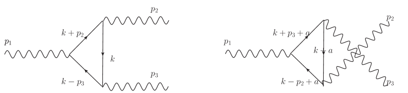
Figure 2: Diagrams relevant for the $Z^{\prime}VV$ vertex function calculation. The integration variable $k$ of one diagram can be shifted with respect to another by an arbitrary momentum $a$.

The calculation of the $Z^{\prime}VV$ vertex function involves the calculation of the pair of diagrams shown in Fig. 2, where we understand the sum over all the fermions charged under the $U(1)^{\prime}$ and the relevant SM gauge group. In an anomaly free theory one can always shift the integration momentum of one diagram with respect to the other by an arbitrary momentum $a_{\mu}$, without changing the finite answer. This is no longer true in an anomalous theory. As we will immediately see the momentum shift $a$ is not arbitrary in our setup, and in fact for a given Wess-Zumino counterterm it will be completely determined by the required gauge invariance of the EW group.

Our objective is to make sure that only the gauge transformation of the effective action with respect to the $U(1)^{\prime}$ does not vanish, which is equivalent to the requirement that the Ward (Slavnov-Taylor) identities for the EW gauge group hold. Namely, in the case of the unbroken $SU(2)_{L}\times U(1)_{Y}$ we get

$$p_{\mu}\Gamma_{\text{3-point}}^{\mu\nu\rho}=0$$ (9)

when $p_{\mu}$ is the momentum of the SM gauge boson, which would correspond to $p_{2}$ and $p_{3}$ in Fig. 2. When we will move to the broken EW symmetry, Eq. (9) will be accompanied by an extra piece, corresponding to the Goldstone boson contribution, that we will take care of later.

When we are dealing with the mixed anomaly, the expression that one gets in (9) is $a_{\mu}$-dependent. Because the anomalies do not cancel out, each separate term of $\Gamma^{\mu\nu\rho}_{\text{3-point}}$ is nominally linearly divergent. Therefore, because of the freedom to shift the integration momentum by $a_{\mu}$, we expect the Ward identity to have a form

$$p_{\mu}\Gamma^{\mu\nu\rho}\sim\int d^{4}k\left(f^{\mu\nu\rho}(k_{\sigma}+a^{\prime}_{\sigma})-f^{\mu\nu\rho}(k_{\sigma})\right)~{},$$ (10)

with the leading term of $f^{\mu\nu\rho}$ in $k$ leading to the linear divergence of the integral. Note, that generically the shift momentum $a^{\prime}$ need not be exactly equal to $a$, but rather can involve a linear combination of the external momenta as well. After expanding the first term we find that the result does not vanish, but rather reduces to a surface term

$$2i\pi^{2}a^{\prime\sigma}\lim_{k^{2}\to\infty}k^{2}k_{\sigma}f^{\mu\nu\rho}(k)~{},$$ (11)

which is finite and $a$-dependent. There is no choice of $a_{\mu}$ to set the Ward identities in Eq. 10 to zero simultaneously for all three incoming momenta $p_{i}$ in Fig. 2. However, there is always a choice of $a_{\mu}$ that preserves the Ward identities of the electroweak gauge group. This is exactly the choice we will proceed with.

It is also worth noting that there is in fact a one-to-one correspondence between the Wess-Zumino counterterm (and, consequently $C_{1}-C_{N}$ combination in Eqs. (7) and (8)) and the momentum shift $a$ that we are required to choose. If we choose the counterterm such that $C_{N}$ vanishes, and consequently, the effective action is invariant under the $SU(N)$ transformation (that we identify with the EW group transformation), we will not need any momentum shift between the two diagrams to restore gauge invariance. This is because the counterterm is imposing EW gauge invariance already. On the other hand, if we are not enforcing gauge invariance at the Lagrangian level with an appropriate Wess-Zumino counterterm, we are obliged to do it by choosing a non-trivial momentum shift, so that eventually all the three (and higher) point functions of the theory are well defined. In all of our further calculations we will set the counterterm to zero and calculate the necessary momentum shift to restore gauge invariance.

Finally, we briefly comment on the restoration of gauge invariance of the spontaneously broken gauge theory, that is the case in the EW group, and is relevant for the calculation of the 3-point function of the $Z^{\prime}$ with $W$ and $Z$ bosons. In principle, we use exactly the same procedure that we have described before, except that when calculating the Ward identities, we have to include the piece contributed by the Goldstone boson. Further details of this procedure are described in Ref. Racioppi:2009yxa . Practically, instead of Eq. (9) we must demand

$$-ip_{\mu}\Gamma^{\mu\nu\rho}+m_{V}\Gamma^{\nu\rho}_{\text{NG}}=0$$ (12)

where $\Gamma^{\nu\rho}_{\text{NG}}$ stands for the three-point function with the gauge boson $V_{\mu}$ replaced by its corresponding Goldstone boson.

3 Dark Matter Models with Heavy Anomalous $Z^{\prime}$

In this section we describe in more detail the dark matter models with $Z^{\prime}$ mediated interactions that we will consider. As we outline these models, we will make no requirement that the low-energy fermion content of our theory cancels all the gauge anomalies. This is a common step in the DM literature, which typically assumes that extra fermions, resolving anomaly cancellation, appear at high scales. Below the mass scale of these fermions we get an effective field theory similar to the one that we have formulated in the previous section.

We begin with a SM singlet Majorana fermion $\chi$ that couples axially to the gauge boson $Z^{\prime}$ of some new $U(1)^{\prime}$ symmetry. The choice of this setup is mostly motivated by the null results of DM direct detection experiments. The vectorial couplings of the Majorana fermion to the $Z^{\prime}$ are naturally precluded and therefore the scattering in the direct detection experiments is either spin-dependent or velocity-suppressed at tree level. The spin and velocity independent interactions are often negligible. Because the DM is not charged under the SM gauge groups, it has no impact on the mixed anomalies, in which we are mostly going to be interested in order to calculate the DM annihilations into SM particles.

While Majorana particles, being real fields, cannot be charged under an exact Abelian group, they can couple to the gauge boson if the gauge group is broken. In the latter case the fermions get their masses via the Higgs mechanism (e.g. via couplings like $\sim\Phi\psi\psi$), or, in the case of vector-like fermions, as a result of mixing with other singlet fermions. Because of the possible mixing effects, the coupling of $Z^{\prime}$ to DM need not be equal to the coupling to the SM.

In general, the $U(1)^{\prime}$ will be anomalous without the introduction of additional fermions besides $\chi$. Indeed, gauging any flavor-universal symmetry other than $B-L$, $Y$-sequential or linear combination thereof, leads to mixed anomalies between the gauge groups of the SM and the new $U(1)^{\prime}$. These must be resolved by new fermions with non-trivial SM charge. Here we do not try to build a full UV-complete model (for explicit attempts to do this see e.g. Ismail:2016tod ; Ellis:2017tkh ), as for our purposes the only relevant quantities are the anomaly coefficients in the EFT that solely include the SM, $\chi$, and $Z^{\prime}$. At sufficiently high energies, above the cutoff $\Lambda$ (see Sec. 2), all gauge anomalies must cancel.

As we are interested in the effects of anomalies, it is interesting to consider explicit models and discern the phenomenological importance of the effects of the $Z^{\prime}$ couplings to the gauge bosons. The first model we will be concerned with is one where the SM fermions are axially charged under $U(1)^{\prime}$. In choosing this particular case we are mostly motivated by the vast existing literature on DM simplified models, that usually assumes a $U(1)^{\prime}$ with pure axial charges as a standard benchmark point Lebedev:2014bba ; Boveia:2016mrp ; Albert:2017onk . This choice however comes with its own obvious shortcoming, that eventually renders it somewhat non-generic compared to the landscape of other options.

For a SM fermion $f$ the usual SM Yukawa coupling $y_{f}H\bar{f}f$ is gauge invariant only if the Higgs doublet also has dark charge Bell:2016uhg . If $H$ is charged under $U(1)^{\prime}$, in turn, then the $Z^{\prime}$ acquires at least some mass from electroweak symmetry breaking and mixes with the $Z$. This $Z$-$Z^{\prime}$ mixing is constrained by electroweak precision, and even though it can be viable if the $Z^{\prime}$ mass is heavier than a few TeV Jacques:2016dqz , we prefer to avoid these complications, which would defocus us from the goal of showing the phenomenological impact of anomaly-induced interactions. If we assume that the SM Higgs is not charged under the $U(1)^{\prime}$, the only option is to promote the Yukawa couplings to $U(1)^{\prime}$ spurions, by writing the Yukawa terms as

$$\left(\frac{\langle\Phi\rangle}{M_{*}}\right)^{2n}\tilde{y}_{f}H\bar{f}f~{},$$ (13)

where $\langle\Phi\rangle$ is the vacuum expectation value of a field $\Phi$ that spontaneously breaks $U(1)^{\prime}$, $M_{*}$ is some suppression scale dictated by the UV completion, and $n$ is the ratio of the fermion axial $U(1)^{\prime}$ charge to the $\Phi$ charge. In this framework, the natural size of the Yukawa couplings is driven by the size of $\langle\Phi\rangle/M_{*}$. Although this approach is generally consistent with the smallness of the SM Yukawas, it becomes difficult to reproduce the top Yukawa coupling in this way. To “fix” this problem we assume that the top quark couples vectorially to the $Z^{\prime}$. The other fermions are taken to have axial couplings, except for the neutrinos which necessarily have purely left-handed couplings. We will further call this particular symmetry $U(1)_{\text{ax}}^{\prime\,c_{V}^{t}}$.

As with the scalar that could be responsible for a DM Majorana mass term, the particular characteristics of the scalars that generate SM fermion Yukawas are not relevant to the interactions at hand. For our purposes, the only other effect of the scalars which acquire $U(1)^{\prime}$-breaking vacuum expectation values is to provide mass to the $Z^{\prime}$. We simply parametrize these effects by a mass term $\frac{1}{2}m_{Z^{\prime}}^{2}(Z^{\prime})^{2}$, and generally ignore the details of the scalar sector from here on.

In order to summarize these considerations and to fix our notation, we show here the newly added terms to the Lagrangian:

$$\mathcal{L}_{\text{DM}}=-\frac{1}{4}Z^{\prime}_{\mu\nu}Z^{\prime\,\mu\nu}+\frac{1}{2}m_{Z^{\prime}}^{2}Z^{\prime\,2}_{\mu}+\frac{1}{2}\overline{\chi}(i\not{\partial}-m_{\chi})\chi\\ +\frac{1}{2}g_{\chi}Z^{\prime\,\mu}\overline{\chi}\gamma_{\mu}\gamma_{5}\chi+g_{Z^{\prime}}Z^{\prime}_{\mu}\sum_{f}\overline{f}\,\left(g_{V}^{f}\gamma^{\mu}+g_{A}^{f}\gamma^{\mu}\gamma_{5}\right)\,f\,,$$ (14)

where the coupling of the $Z^{\prime}$ to the SM fermions $f$ is given by $g_{Z^{\prime}}$ times the charges $g_{V}^{f}$ and $g_{A}^{f}$, which are given in Table 1, and $g_{\chi}$ is the coupling to the Majorana DM $\chi$.

It is easy to note in what sense this “modified axial model” $U(1)_{\text{ax}}^{\prime\,c_{V}^{t}}$ is not generic. If we do not tighten the solution of the flavor problem with the DM theory (which is possible but by no means necessary) yet still insist that the SM Higgs is uncharged under the new force, the charges of the SM fermions are vectorlike under the $U(1)^{\prime}$. This immediately implies that the mixed anomalies with the $U(1)_{\text{EM}}$ and the SM color group must vanish. At sufficiently large DM masses this strongly suppresses the $\gamma\gamma$ and $gg$ annihilation channels of the DM, but does not qualitatively change other channels. As an example of this model we choose $U(1)^{\prime}_{B+L}$, which is simply one representative point in a large class of models.

Finally we choose to also show a leptophilic model (for this purpose, $U(1)^{\prime}_{L}$). This choice is special because we have no constraints from the LHC and direct detection, and all the constraints come from indirect detection searches.

	$SU(3)$	$SU(2)$	$U(1)_{Y}$	$U(1)_{B-L}$	$U(1)_{\text{ax}}^{\prime\,c_{V}^{t}}$	$U(1)^{\prime}_{B+L}$	$U(1)^{\prime}_{L}$
$\begin{pmatrix}\nu^{e}_{L}\\ e^{i}_{L}\end{pmatrix}$, $\begin{pmatrix}\nu^{\mu}_{L}\\ \mu^{i}_{L}\end{pmatrix}$, $\begin{pmatrix}\nu^{\tau}_{L}\\ \tau^{i}_{L}\end{pmatrix}$	1	2	$-\tfrac{1}{2}$	$-1$	$-1$	$+1$	$+1$
$\left(e^{i}_{R}\right)^{\text{C}}$, $\left(\mu^{i}_{R}\right)^{\text{C}}$, $\left(\tau^{i}_{R}\right)^{\text{C}}$	1	1	$1$	$+1$	$-1$	$-1$	$-1$
$\begin{pmatrix}u_{L}\\ d_{L}\end{pmatrix}$, $\begin{pmatrix}c_{L}\\ s_{L}\end{pmatrix}$	3	2	$\tfrac{1}{6}$	$+\tfrac{1}{3}$	$-1$	$+\tfrac{1}{3}$	$0$
$\left(u_{R}\right)^{\text{C}}$, $\left(c_{R}\right)^{\text{C}}$	$\overline{\textbf{3}}$	1	$-\tfrac{2}{3}$	$-\tfrac{1}{3}$	$-1$	$-\frac{1}{3}$	$0$
$\left(d_{R}\right)^{\text{C}}$, $\left(s_{R}\right)^{\text{C}}$	$\overline{\textbf{3}}$	1	$\tfrac{1}{3}$	$-\tfrac{1}{3}$	$-1$	$-\tfrac{1}{3}$	$0$
$\begin{pmatrix}t_{L}\\ b_{L}\end{pmatrix}$	3	2	$\tfrac{1}{6}$	$+\tfrac{1}{3}$	$-1$	$+\tfrac{1}{3}$	$0$
$\left(t_{R}\right)^{\text{C}}$	$\overline{\textbf{3}}$	1	$-\tfrac{2}{3}$	$-\tfrac{1}{3}$	$+1$	$-\tfrac{1}{3}$	$0$
$\left(b_{R}\right)^{\text{C}}$	$\overline{\textbf{3}}$	1	$\tfrac{1}{3}$	$-\tfrac{1}{3}$	$-1$	$-\tfrac{1}{3}$	$0$
Higgs $\begin{pmatrix}\phi^{+}\\ \phi^{0}\end{pmatrix}$	1	2	$\frac{1}{2}$	$0$	$0$	$0$	$0$

Table 1: Charges of the SM matter content under some choices of $U(1)^{\prime}$ that we further analyze in the paper.

Taking all this into account we present the charges of the SM fields under the new $U(1)^{\prime}$s in Table 1. For comparison, we also show $B-L$, which is of course anomaly free and does not require any extra terms in the effective action.

Since our axial vector model features flavor non-universal $Z^{\prime}$ quark couplings, we parenthetically consider here the flavor constraints on this kind of $Z^{\prime}$. Even though the axial-$Z^{\prime}$ couplings are diagonal in the flavor basis, the quark rotations that diagonalize the Yukawa matrix generally induce off-diagonal couplings between quark mass eigenstates Abdallah:2015ter . To estimate the size of the associated flavor-changing neutral currents (FCNCs), we must make assumptions about the structure of the quark rotations. Note that the only measured misalignment between the quark flavor and mass eigenstates is from the CKM matrix $V_{\mathrm{CKM}}$, which is a combination of the two left-handed quark rotations. Conversely, the $U(1)_{\text{ax}}^{\prime\,c_{V}^{t}}$ model only contains non-universality in the right-handed up-quark sector. Of course, if the mixing angles in the RH sectors are completely anarchical, the structure that we discuss is not viable. However, this is not the only option, especially if we take into account the hierarchical structure of $V_{\mathrm{CKM}}$. First, FCNCs may be completely avoided if the right-handed quark flavor and mass eigenstates are identical (this would invoke either a fine-tuning or some other structure that would explain the vanishing rotation angles).

Alternatively, let us assume that the flavor structures of the RH and LH quark sectors are similar, such that the product of the rotations between the up- and down-type RH quark U(1)’ flavor and mass eigenstates is $\sim V_{\mathrm{CKM}}$. Then, since the non-universality is only in the third generation, the $Z^{\prime}\bar{c}_{R}u_{R}$ coupling will go as $\sim V_{\mathrm{CKM}}^{ub*}V_{\mathrm{CKM}}^{cb}$, which is quite small, without dangerous consequences for $D$ mixing. Non-universal couplings in the down-type sector are also induced at the loop level, leading to effects such as $B-\overline{B}$ mixing.

Finally we note that a kinetic mixing term $B_{\mu\nu}F^{\prime\mu\nu}$, where $B$ and $F$ are the $U(1)_{Y}$ and $U(1)^{\prime}$ field strengths respectively, is fully allowed by the symmetries of the theory. Sizable kinetic mixing can lead to observable effects that are interesting but separate from those caused by the triple gauge vertices induced by anomalies. We henceforth assume negligible mixing, and concentrate on the anomalous couplings among the SM and $U(1)^{\prime}$ gauge bosons.

4 Application to Dark Matter Models

In this section we present the main results of our paper. First, we will use the results of Sec. 2 to explicitly calculate the annihilation cross sections of the DM particle into the SM gauge bosons. In the following subsections we show the prospects for the direct and indirect detection, as well as LHC searches. We will emphasize the complementarity of these searches to properly analyze the possible parameter space of these models.

4.1 Annihilation cross sections into the SM gauge bosons

The objective in this part of our paper is to explicitly calculate the relevant annihilation cross sections that arise only at the one-loop level. To begin, we outline the calculation of the coupling between three gauge bosons induced by anomalies, starting with the $Z^{\prime}$-$\gamma$-$\gamma$ vertex. We take a single fermion $f$ of electric charge $Q_{f}^{em}$ to run in the loop diagrams of Fig. 2, whose amplitude we write as $\epsilon_{\mu}(p_{1})\epsilon^{*}_{\nu}(p_{2})\epsilon^{*}_{\rho}(p_{3})\Gamma^{\mu\nu\rho}$. Note that we use $p_{1}$ for the $Z^{\prime}$ momentum, while the momenta $p_{2},\ p_{3}$ stand for the photon momenta. If the fermion’s $U(1)^{\prime}$ coupling is vectorial, then by Furry’s theorem the vertex vanishes. Without loss of generality we assume a $Z^{\prime}f\bar{f}$ vertex with strength $ig_{Z^{\prime}}\gamma^{\mu}(g_{V}+g_{A}\gamma^{5})$ with the understanding that only $g_{A}$ will contribute. As described in Sec. 2, contracting the external gauge boson momenta with the triangle amplitude gives non-vanishing results due to surface terms (see Preskill:1983 ; Racioppi:2009yxa for further calculation details). The resulting Ward identities depend, as explained in Sec. 2, on the loop momentum shift $a$:

$$(p_{1})_{\mu}\Gamma^{\mu\nu\rho} = \frac{g_{Z^{\prime}}e^{2}g_{A}(Q_{f}^{em})^{2}}{8\pi^{2}}\epsilon^{\nu\rho\alpha\beta}a_{\alpha}(p_{1})_{\beta}$$

$$(p_{2})_{\nu}\Gamma^{\mu\nu\rho} = \frac{g_{Z^{\prime}}e^{2}g_{A}(Q_{f}^{em})^{2}}{8\pi^{2}}\epsilon^{\mu\rho\alpha\beta}(a+2p_{3})_{\alpha}(p_{2})_{\beta}$$ (15)

$$(p_{3})_{\rho}\Gamma^{\mu\nu\rho} = \frac{g_{Z^{\prime}}e^{2}g_{A}(Q_{f}^{em})^{2}}{8\pi^{2}}\epsilon^{\mu\nu\alpha\beta}(a-2p_{2})_{\alpha}(p_{3})_{\beta}$$

At this stage we can either tune the Wess-Zumino conterterm to get rid of any $a_{\mu}$ dependence in these expressions or, alternatively, set the Wess-Zumino counterterm to zero and find an appropriate momentum shift to maintain the necessary Ward identities. We choose the latter recipe to resolve this problem. We make the phenomenologically motivated choice of retaining $U(1)_{\text{EM}}$ gauge invariance, which corresponds to the requirement that the second and third lines of Eq. (4.1) vanish. This, in turn, may be accomplished by setting $a=2(p_{2}-p_{3})$, yielding the Ward identities

$$(p_{1})_{\mu}\Gamma^{\mu\nu\rho} = \frac{g^{\prime}e^{2}Q_{f}(Q_{f}^{em})^{2}}{2\pi^{2}}\epsilon^{\nu\rho\alpha\beta}(p_{2})_{\alpha}(p_{3})_{\beta}$$

$$(p_{2})_{\nu}\Gamma^{\mu\nu\rho} = (p_{3})_{\rho}\Gamma^{\mu\nu\rho}=0$$ (16)

Next, to calculate the relevant cross section, we write the most general form of the amplitude using the standard Rosenberg parametrization Rosenberg:1962pp

$$\Gamma^{\mu\nu\rho} = \frac{g_{Z^{\prime}}e^{2}g_{A}(Q_{f}^{em})^{2}}{\pi^{2}}\Big{(}I_{1}\epsilon^{\alpha\nu\rho\mu}(p_{2})_{\alpha}+I_{2}\epsilon^{\alpha\nu\rho\mu}(p_{3})_{\alpha}$$

$$\ +\ I_{3}\epsilon^{\alpha\beta\nu\mu}(p_{2})^{\rho}(p_{2})_{\alpha}(p_{3})_{\beta}+I_{4}\epsilon^{\alpha\beta\nu\mu}(p_{3})^{\rho}(p_{2})_{\alpha}(p_{3})_{\beta}$$

$$\ +\ I_{5}\epsilon^{\alpha\beta\rho\mu}(p_{2})^{\nu}(p_{2})_{\alpha}(p_{3})_{\beta}+I_{6}\epsilon^{\alpha\beta\rho\mu}(p_{3})^{\nu}(p_{2})_{\alpha}(p_{3})_{\beta}\Big{)}$$

where $I_{i},1\leq i\leq 6$ are form factors to be computed. By dimensional analysis, it is clear that the effect of any divergences must be in $I_{1}$ and $I_{2}$, while the remaining form factors are finite. We thus use the Ward identities of Eq. (4.1) to fix the divergent form factors, and calculate the others explicitly. The final result is Racioppi:2009yxa

$$I_{1}(p_{2},p_{3};m_{f}) = (p_{2}\cdot p_{3})I_{3}(p_{2},p_{3};m_{f})+p_{3}^{2}I_{4}(p_{2},p_{3};m_{f})$$

$$I_{2}(p_{2},p_{3};m_{f}) = -I_{1}(p_{3},p_{2};m_{f})$$

$$I_{3}(p_{2},p_{3};m_{f}) = -C_{12}(p_{3}^{2},p_{1}^{2},p_{2}^{2},m_{f}^{2},m_{f}^{2},m_{f}^{2})$$ (18)

$$I_{4}(p_{2},p_{3};m_{f}) = C_{11}(p_{3}^{2},p_{1}^{2},p_{2}^{2},m_{f}^{2},m_{f}^{2},m_{f}^{2})+C_{1}(p_{3}^{2},p_{1}^{2},p_{2}^{2},m_{f}^{2},m_{f}^{2},m_{f}^{2})$$

$$I_{5}(p_{2},p_{3};m_{f}) = -I_{4}(p_{3},p_{2};m_{f})$$

$$I_{6}(p_{2},p_{3};m_{f}) = -I_{3}(p_{2},p_{3};m_{f})$$

where the $C$ functions are Passarino-Veltman loop functions Hahn:1998yk . When there are multiple fermions charged under both electromagnetism and $U(1)^{\prime}$, Eq. (4.1) is readily generalized by summing over the available loop fermions.

The above vertex may now be used to calculate physical observables. For instance, the amplitude for DM annihilation to photons immediately follows, and the resulting cross section takes a rather compact form

$$\sigma(\chi\chi\to\gamma\gamma)=\frac{\alpha_{\text{em}}^{2}g_{\chi}^{2}g_{Z^{\prime}}^{4}}{\pi^{3}}\frac{m_{\chi}^{2}\sqrt{s}}{m_{Z^{\prime}}^{4}\sqrt{s-4m_{\chi}^{2}}}\times\Bigg{|}\sum_{f}c_{A}^{f}N_{c}^{f}Q_{f}^{2}\Big{[}2m_{f}^{2}C_{0}(0,0,s,m_{f}^{2},m_{f}^{2},m_{f}^{2})+1\Big{]}\Bigg{|}^{2}\,,$$ (19)

where the explicit form of the Passarino-Veltman function involved is

$$C_{0}(0,0,s,m_{f}^{2},m_{f}^{2},m_{f}^{2})=\frac{1}{2s}\log^{2}\Bigg{(}\frac{\sqrt{s(s-4m_{f}^{2})}+2m_{f}^{2}-s}{2m_{f}^{2}}\Bigg{)}\,.$$ (20)

This should be compared to the cross section for DM annihilation to fermions,

$$\sigma(\chi\chi\to f\bar{f})=\frac{g_{\chi}^{2}g_{Z^{\prime}}^{4}\,N_{c}^{f}}{3\pi s\big{(}(s-m_{Z^{\prime}}^{2})^{2}+\Gamma_{Z^{\prime}}^{2}m_{Z^{\prime}}^{2}\big{)}}\sqrt{\frac{s-4m_{f}^{2}}{s-4m_{\chi}^{2}}}\Bigg{(}g_{V}^{2}(s-4m_{\chi}^{2})(s+2m_{f}^{2})\\ \ +\ g_{A}^{2}\bigg{(}s(s-4m_{\chi}^{2})+4m_{f}^{2}\Big{(}m_{\chi}^{2}\Big{(}7-6\frac{s}{m_{Z^{\prime}}^{2}}+3\frac{s^{2}}{m_{Z^{\prime}}^{4}}\Big{)}-s\Big{)}\bigg{)}\Bigg{)}\,.$$ (21)

The key difference between these cross sections is that the annihilation to photons remains constant with increasing center-of-mass energy, unlike the annihilation to fermions which eventually falls as $1/s$. Of course this “constant” annihilation rate cannot proceed to arbitrarily high energy because it would eventually break the unitarity of the theory. We will comment on this issue later in the section.

We calculate the form factors for the annihilations into the rest of the gauge bosons, using exactly the machinery that we have shown here. We list the relevant results in Appendix A. For simplicity we take the $Z^{\prime}$ width to be $\Gamma_{Z^{\prime}}=m_{Z^{\prime}}/10$ throughout our calculations. This choice only affects the extent of the influence of resonant effects in our results.

Before we present our results, it is instructive to see how the annihilation cross sections $\sigma v$ scale with the kinetic energy of the fermions for fixed DM mass. We show this scaling within the EFT on Fig. 3 (we use for this illustration the $U(1)_{\text{ax}}^{\prime\,c_{V}^{t}}$ model). While the cross sections into the fermions fall at the high energies as $1/s$ (as one would expect), the annihilations into the gauge bosons stay constant as a function of $s$, signaling an inevitable breakdown of unitarity at high energies. This breakdown is expected from the way we have formulated our EFT in Sec. 2, in particular because of the higher dimensional interactions that we were forced to introduce. Of course these cross sections are tamed at the scale where the spectator fermions show up. This can in turn happen at or below the scale $\Lambda$ as defined in Eq. (5) (modulo replacing the Abelian anomaly by a mixed one).

Note also that unitarity will often dominate the exact bound on the cutoff $\Lambda$, although it will often be of order (5). For example, a simple back-of-the-envelope estimation leads us to the conclusion that the unitarity of the model depicted on Fig. 3 will break down at a scale $\sim 100$ TeV. In this sense the very right corner of this plot is not meaningful and the physics there should be described by a full UV complete theory rather than the EFT.

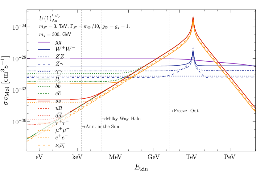
Figure 3: Annihilation cross sections in the $U(1)_{\text{ax}}^{\prime\,c_{V}^{t}}$ model as a function of the DM kinetic energy within the EFT that we describe. The blue curves indicate gauge boson final states that receive contributions from anomalies. Annihilations into heavy quarks, light quarks, and leptons are shown in green, red, and yellow, respectively. Kinetic energies corresponding to DM in the Sun, the Milky Way halo, and at freezeout are indicated. Note that above the scale $\sim 100$ TeV the EFT cannot give the correct solution due to the inevitable unitarity breakdown.

Note also the difference between the fermions that couple axially and ones that couple vectorially to the $Z^{\prime}$. While annihilations into the former final states (in this particular example, all the SM fermions except the top) are constant at low energies, the latter in this range scale as $v^{2}$, and therefore linearly with the kinetic energy. This can also be clearly observed in Eq. (21).

Another important lesson that we learn from Fig. 3 is the dominance of the various channels in different physical situations. For example, the velocity is still high enough during the thermal freeze-out to render the annihilation into the gauge bosons unimportant, such that the relic abundance is determined almost completely by the annihilations into the fermions. However at lower velocities (annihilation in the Galactic halo or at the center of the Sun) the entire signal is essentially determined by the radiative annihilations into the gauge bosons.

Finally let us notice, that even in the models where the respective mixed anomaly vanishes, the annihilation channels into the gauge bosons are induced by finite radiative corrections. However, because these contributions do not grow with energy, they are much smaller than the anomaly-augmented annihilations, and can be neglected.

4.2 Relic abundance

We first briefly comment on the DM relic abundance, if we assume that the DM is the thermal relic (which might or might not be the case). WIMP freezeout typically happens near $x=m_{\chi}/T\approx 25$, with the particular decoupling temperature only logarithmically sensitive to the annihilation cross section. The annihilation channels which determine the relic abundance are thus simply the modes which dominate at a DM velocity of $\sqrt{\frac{3}{x}}\sim 1/3$. From Fig. 3, it is apparent that DM annihilation to fermions is primarily responsible for setting the relic abundance. Consequently, the impact of anomalies in the DM relic density calculation is minimal. We thus expect the values of the couplings and masses that reproduce the observed DM abundance to be similar to previous calculations in the literature, see e.g. Arcadi:2017kky .

4.3 Indirect detection

Today very little kinetic energy is available for DM annihilation because the typical velocity of a DM in the Milky Way halo is $\sim 10^{-3}$. In our models the gauge boson modes can dominate the annihilations, and so the DM can be probed through searches for annihilation to $gg$, $W^{+}W^{-}$, $\gamma\gamma$, $Z\gamma$ and $ZZ$.

We illustrate this point on Fig. 4, where we show the branching ratios into the various annihilation channels of the DM in our galaxy as a function of the DM mass. If the DM is relatively light, $\sim 10$ GeV, the BRs are dominated by the fermionic channels, particularly $b\bar{b}$. However at sufficiently high DM masses the $gg$ (if the mixed anomaly of the $U(1)^{\prime}$ with the SM does not vanish) and $W^{+}W^{-}$ channels dominate the annihilations at such low DM velocities, and therefore the indirect detection signatures. We also point out the importance of the $\gamma\gamma$ (when present) and $Z\gamma$ annihilation channels. Although the latter channels are heavily suppressed compared to the $W^{+}W^{-}$, the photon emission is monochromatic, leading to the prediction of a $\gamma$ ray line.

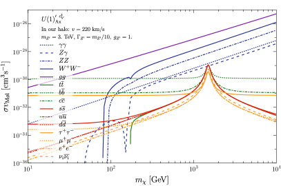
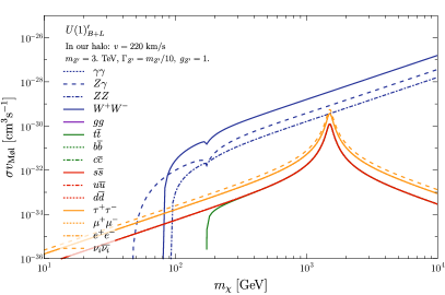
Figure 4: Left: DM mass vs. annihilation branching ratios in the $U(1)_{\text{ax}}^{\prime\,c_{V}^{t}}$ model. The DM velocity is taken to be 220 km/s, characteristic of the Milky Way halo. The curves are colored as in Fig. 3. Right: same for the $U(1)^{\prime}_{B+L}$ model. The quark lines all overlap on the red line. The branching ratios of the $U(1)^{\prime}_{L}$ model are analogous to the ones of $U(1)^{\prime}_{B+L}$, without the quark channels.

4.3.1 Gamma ray continuum searches

We first consider limits from the continuum $\gamma$ ray spectrum, where the strongest current bound comes from dSph Fermi-LAT observations Drlica-Wagner:2015xua ; Ackermann:2015zua and, for TeV scale DM masses, from HESS observation of the continuum emission from the Galactic Center Abdallah:2016ygi .

These bounds depend on the products of DM annihilation, as different SM particles yield distinct photon spectra. In order to apply the $\gamma$ ray limits, we thus consider the annihilation branching ratios to different final states. At low DM mass, the fermionic annihilation channels are dominant, as seen in Fig. 4.

We start by discussing the $U(1)_{\text{ax}}^{\prime\,c_{V}^{t}}$ model, where all such channels except for $t\bar{t}$ are chirally suppressed, and the $b\bar{b}$ and $\tau^{+}\tau^{-}$ annihilations are more common than those into the light fermions. In practice, the limits on annihilations to $b\bar{b}$ and $\tau^{+}\tau^{-}$ are quite close to one another Ackermann:2015zua . Similarly, DM annihilations to charm quarks produce similar photon spectra as to up quarks Cirelli:2010xx , for which the limits are in turn close to those for annihilations to $b\bar{b}$. We thus choose to compare the total fermionic annihilation cross section to the Fermi-LAT limit on DM annihilating to bottom quarks for DM masses below approximately 200 GeV.

At larger DM masses, the $gg$, $W^{+}W^{-}$ and $ZZ$ channels take over. Again, since the resulting $\gamma$ ray spectra from these annihilation modes are similar, we simply compare the total bosonic annihilation cross section to the Fermi-LAT limit on DM annihilations to $W^{+}W^{-}$ (which gives a slightly weaker bound than $gg$). Finally, in the resonance region $m_{\chi}\approx m_{Z^{\prime}}/2$, fermionic annihilations take over again and we switch back to comparing the total annihilation cross section to the $b\bar{b}$ limit from Fermi-LAT once more. Throughout, we assume that $\chi$ makes up all of the observed DM.

In the $U(1)^{\prime}_{B+L}$ and $U(1)^{\prime}_{L}$ models the procedure is analogous, with the notable difference that the $gg$ channel disappears. At low DM masses the annihilations to fermions, which now couple vectorially to the $Z^{\prime}$, are velocity suppressed.

We show the bounds on the suppression scale $m_{Z^{\prime}}/\sqrt{g_{Z^{\prime}}g_{\chi}}$ in the three models as a function of the DM mass in Fig. 5. These bounds are insensitive to the choice of DM profile Ackermann:2015zua . The bound on the $U(1)_{\text{ax}}^{\prime\,c_{V}^{t}}$ model is significantly stronger than those on the $B+L$ and $L$ models because of the dominance of the $gg$ annihilation channel, which is prolific in $\gamma$ rays due to its secondary production of pions. As the mixed anomaly of the latter two $U(1)$s with the color group vanishes, the annihilations into $gg$ in these models are much more modest.

The choice of the mediator mass has no effect on the bounds except in the resonance region, and so while the limits correspond to somewhat large couplings for the indicated $m_{Z^{\prime}}$. Lighter mediators will have similar constraints. Note that if the DM is significantly heavier than the mediator mass, the coupling $g_{\chi}$ should be sufficiently small to avoid unitarity constraints on the DM self-scattering Kahlhoefer:2015bea .

We show the HESS continuum Galactic Center bounds in Fig. 5, assuming three different DM profiles (see Sec. 4.3.2 for more details). For each profile we compute the integrated J-factor between 0.3° and 1° around the direction of the Galactic Center using the tables from Cirelli:2010xx and scale the HESS bound appropriately.

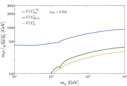
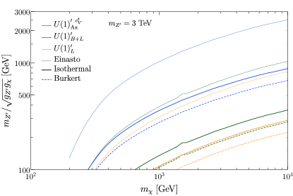
Figure 5: Limits from continuum $\gamma$ ray emission on the three models we consider. Left: bounds from Fermi-LAT observations of dSphs Drlica-Wagner:2015xua ; Ackermann:2015zua . Right: bounds from HESS observation of the Galactic Center Abdallah:2016ygi , for three choices of the DM profile distribution.

4.3.2 Gamma ray line searches

Given the potential for annihilation to $\gamma\gamma$ or $Z\gamma$ through anomalies, we now discuss the impact of $\gamma$ ray line searches on our benchmark models, as performed by Fermi-LAT Ackermann:2015lka and HESS Abramowski:2013ax . Fermi-LAT is typically sensitive to photons below several hundred GeV in energy, while HESS, being a terrestrial telescope, has the best sensitivity for much more energetic $\gamma$ rays.

The bounds from line searches generally depend on the DM halo profile, and so we will show their variation when different profiles are considered; for an overview of DM halo profiles see for instance Ref. Lisanti:2016jxe . Fermi-LAT optimizes the signal region of interest to maximize the bound depending on the profile, for several different halo shape choices. For instance, the optimal bound is obtained for a region subtending 16° around the galactic center for the Einasto profile, but 90° for an isothermal profile. HESS only shows limits for the Einasto profile, using a signal region of radius 1°. We choose to show bounds for Einasto, isothermal and Burkert DM halo profiles, by rescaling the Fermi-LAT and HESS limits using the ratios of J-factors for different profiles over the signal regions of interest Cirelli:2010xx . In the case of Fermi-LAT, we obtain the limit for a Burkert profile by rescaling the constraint for an isothermal profile, as these halo shapes are both relatively cored.

We further calculate the expected annihilation cross section to photons and compare with the Fermi-LAT and HESS $\gamma$ ray line search bounds, computed as described above for different halo profiles. We notice that even if the $\gamma\gamma$ channel is absent (up to finite terms that we neglect here) because of the vanishing mixed anomaly with the $U(1)_{\text{EM}}$, as is the case for $U(1)^{\prime}_{B+L}$ and $U(1)^{\prime}_{L}$, the $Z\gamma$ channel can be present, because it is controlled by the mixed anomaly with the hypercharge. Most monochromatic photons come from DM annihilation to $\gamma\gamma$ when it is present, as the $Z\gamma$ mode is less common and provides half as many photons per annihilation. In the $U(1)_{\text{ax}}^{\prime\,c_{V}^{t}}$ we include the $Z\gamma$ channel above $m_{\chi}\gtrsim 140$ GeV, where the difference in energies between photons from $\gamma\gamma$ and $Z\gamma$ annihilations is expected to be below the resolution of Fermi-LAT; that of HESS is worse. For simplicity, below this threshold we ignore annihilations to $Z\gamma$, which should not significantly affect our final results due to the lower cross section for this channel.

The resulting constraints are presented in Fig. 6, and they clearly illustrate the impact of the anomalies on indirect detection constraints. Conversely, anomaly-free models often do not face meaningful limits from $\gamma$ ray line searches, due to suppressed annihilation cross sections to photons Jacques:2016dqz . In the two models $U(1)^{\prime}_{B+L}$ and $U(1)^{\prime}_{L}$, where only $Z\gamma$ contributes to the signal, the final bound is clearly much weaker, but still non-negligible for a DM mass of a few TeV. The limits are quite sensitive to the choice of halo profile, particularly for HESS which presents limits for a $\gamma$ ray line search in a very narrow region around the Galactic Center. As expected, the best limits are obtained for the cuspy Einasto profile. The sensitivity of line searches is considerably weakened in the resonance region, where annihilation to $\gamma\gamma$ is forbidden due to Landau-Yang theorem and only the $Z\gamma$ mode contributes.

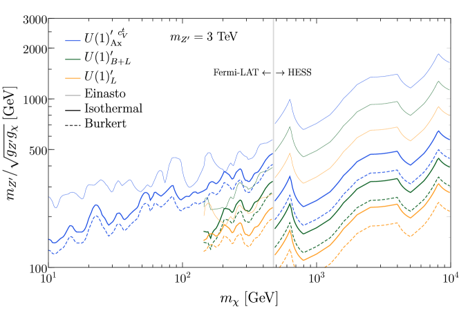
Figure 6: Limits from Fermi-LAT Ackermann:2015lka and HESS Abramowski:2013ax searches for $\gamma$ ray lines. Below (above) DM masses of 500 GeV, Fermi-LAT (HESS) provides the constraint. The choice of mediator mass affects only the resonance region $m_{\chi}\approx m_{Z^{\prime}}/2$.

4.3.3 Neutrino telescopes

We finally consider DM annihilation to neutrinos in the Sun, and the associated bounds from three years of observations of IceCube Aartsen:2016zhm . In particular, annihilations to $W^{+}W^{-}$, $ZZ$ and $\tau^{+}\tau^{-}$ produce high-energy neutrinos which are tightly constrained, while annihilations to $b\bar{b}$ are less strongly limited because of the softer neutrino spectrum. To obtain the limit on the overall annihilation cross section – and hence the scale of DM-SM interactions – in any given model, we must convolve the various IceCube limits on different annihilation channels with the annihilation branching ratios in the model, as we did above for the continuum $\gamma$ ray bounds.

For DM that is captured in the Sun, the typical kinetic energy is of the same order as the temperature at the center of the Sun, $10^{7}~{}\mathrm{K}\sim$ keV, which corresponds to negligible velocity for DM heavier than the MeV scale. At such energies, $p$-wave annihilation is essentially non-existent, and the annihilation branching ratios are similar to those in the Milky Way halo shown previously in Fig. 4.

The IceCube bounds on annihilations into $b\bar{b}$ are weaker than the bounds on annihilations into $\tau^{+}\tau^{-}$ by 2-3 orders of magnitude. Therefore at low DM mass $\tau^{+}\tau^{-}$ annihilations always provide the most constrained source of neutrinos, even in the $U(1)_{\text{ax}}^{\prime\,c_{V}^{t}}$ model when bottom quarks are the main products of DM annihilation.

At higher masses, $W^{+}W^{-}$ and $ZZ$ annihilations face bounds from IceCube that are nearly as strong as $\tau^{+}\tau^{-}$ Aartsen:2016zhm , and annihilations to $Z\gamma$ produce half as many neutrinos as $ZZ$. Thus we use the stronger of the bounds on annihilations to $\tau^{+}\tau^{-}$ and $W^{+}W^{-},ZZ,Z\gamma$, scaling the IceCube limits by the appropriate branching ratios and assuming that the neutrino spectrum for the latter channels are all similar to that for $W^{+}W^{-}$.

The translation of the IceCube bounds on the SD DM-proton scattering cross section $\sigma_{p}^{\text{SD}}$ to bounds on the EFT scale $m_{Z^{\prime}}/\sqrt{g_{Z^{\prime}}g_{\chi}}$ requires some care about the form factor assumed for DM capture in the Sun. When providing a bound on $\sigma_{p}^{\text{SD}}$, IceCube assumes that DM and the SM interact through the NR operator $\mathcal{O}_{4}^{\text{NR}}$ (according to the standard notation, see e. g. DelNobile:2013sia ; Catena:2015uha ). This is indeed the operator that arises in the $U(1)_{\text{ax}}^{\prime\,c_{V}^{t}}$ model, but for the $U(1)^{\prime}_{B+L}$ model, the leading interaction is the SI velocity-suppressed operator $\mathcal{O}_{8}^{\text{NR}}$. To convert between bounds on these operators, we use the capture form factors provided by Catena:2015uha . In the leptophilic model $U(1)^{\prime}_{L}$ the DM capture rate is negligible, given the small momentum exchange between DM and free electrons in the Sun, and the suppressed loop interaction with nucleons, so IceCube bounds do not apply.

The results are shown in Fig. 7. Because the IceCube bounds are sensitive to the branching ratios of DM annihilations rather than to the absolute annihilation cross sections, in the $U(1)_{\text{ax}}^{\prime\,c_{V}^{t}}$ model the bounds are weakened due to the large branching ratio into gluons, which yield a negligible neutrino spectrum. In the $U(1)^{\prime}_{B+L}$ model, while there are no annihilations into gluons, the velocity-suppressed capture rate results in an even looser bound. We will see in the next section that in this model, direct detection bounds are much stronger due to coherent enhancement of the spin-independent scattering cross section.

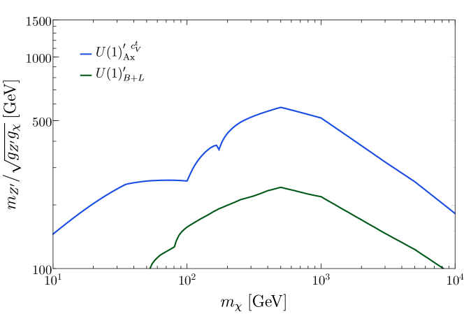
Figure 7: Bounds due to IceCube Aartsen:2016zhm searches for neutrinos originating from DM annihilations in the Sun, on the models we consider.

4.4 Colliders and direct detection

In addition to the above indirect detection searches which can be significantly affected by the presence of anomalies, simplified models of DM face complementary constraints from collider and direct detection experiments. In order to present a complete account of the limits on the models we consider, here we discuss these bounds and compare them to the exclusions derived previously that rely on anomalies.

At the LHC, the main probes of simplified DM models are missing energy-based searches, such as monojets and monophotons, and direct searches for the mediator decaying to SM particles.

The stronger constraints from direct $Z^{\prime}$ searches come from searches for dilepton resonances. We use the combined 8 + 13 TeV CMS dilepton analysis Khachatryan:2016zqb . Because the resonant mediator searches do not involve the DM-mediator coupling, their reach cannot be presented in terms of the DM-SM interaction suppression scale without additional assumptions. Instead, we choose to show in Fig. 8 the upper limit on the $U(1)^{\prime}$ coupling as a function of the mediator mass. The bound on the $U(1)^{\prime}_{B+L}$ model is rescaled to account for the different charge of light quarks in this model. In the leptophilic model $U(1)^{\prime}_{L}$ the LHC bound does not apply, since the production of $Z^{\prime}$ at the LHC is absent at tree level. The bound from the dilepton searches for the $Z^{\prime}$ is quite strong for mediators that are kinematically accessible, and would push us to very low $Z^{\prime}$ couplings to SM fermions.

Figure 8: Bounds from resonant dilepton searches on a $Z^{\prime}$ at LHC from the 8 + 13 TeV combined analysis Khachatryan:2016zqb , presented in the $g_{Z^{\prime}}$-$m_{Z^{\prime}}$ plane for $U(1)_{\text{ax}}^{\prime\,c_{V}^{t}}$ and $U(1)^{\prime}_{B+L}$ ($U(1)^{\prime}_{L}$ is obviously unconstrained).

We also rescale the limits of the 8 TeV CMS monojet search Khachatryan:2014rra for Majorana DM and show the results in Fig. 9. For DM below the TeV scale, monojets provide the dominant bound on the models that we consider.

The LHC monojet analysis clearly does not apply in the $U(1)^{\prime}_{L}$ model, for which we rely on the recast done in Fox:2011fx of the monophoton + missing transverse energy searches performed by the DELPHI collaboration at LEP Abdallah:2003np ; Abdallah:2008aa . Due to the lower energy reach of LEP, the exclusion limit extends up to $m_{\chi}\sim 100$ GeV.

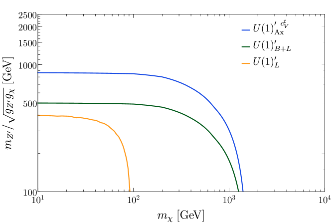
Figure 9: Bounds from the CMS monojet search Khachatryan:2014rra (for the models $U(1)_{\text{ax}}^{\prime\,c_{V}^{t}}$ and $U(1)^{\prime}_{B+L}$), and the monophoton search performed by DELPHI and recast in Fox:2011fx for the $U(1)^{\prime}_{L}$ model.

Two models, out the three we consider, also produce direct detection signatures. The $U(1)_{\text{ax}}^{\prime\,c_{V}^{t}}$ model mainly produces spin-dependent interactions because of the axial couplings. The most powerful direct detection bound for our purposes comes from PICO Amole:2017dex , and is shown in Fig. 10. The bound is comparable to the monojet exclusion limit, and is superseded by Fermi-LAT observations of dSph at DM masses around 500 GeV.

The $U(1)^{\prime}_{B+L}$ model induces instead a spin-independent and velocity-suppressed interaction. The most recent experimental bound comes from XENON-1T Aprile:2017iyp . The collaboration provides a limit obtained assuming that the interaction between DM and nuclei occurs via the canonical spin-independent operator $\mathcal{O}_{1}^{q}$ in the NR EFT of the DM. In our case the dominant interaction is $\mathcal{O}_{6}^{q}$ rather than $\mathcal{O}_{1}^{q}$ Fitzpatrick:2012ix ; Fitzpatrick:2012ib ; Anand:2013yka . We perform a recast by means of the tables provided by DelNobile:2013sia . The result is shown in Fig. 11. The exclusion limit from direct detection is the most powerful for $m_{\chi}$ up to a few TeV, where it is superseded by $\gamma$ ray line searches only if we assume a cuspy profile of the DM density distribution like Einasto.

4.5 Summary of results

The combinations of all the constraints described above are shown in Figs. 10, 11 and 12 respectively for the three models $U(1)_{\text{ax}}^{\prime\,c_{V}^{t}}$, $U(1)^{\prime}_{B+L}$ and $U(1)^{\prime}_{L}$.

Indirect detection provides the strongest bounds at large DM mass, driven by loop annihilations of DM to gauge bosons. Depending on the choice of halo profile, either the HESS $\gamma$ ray line search or the Fermi-LAT dSph continuum $\gamma$ ray spectrum analysis is most constraining in this regime, depending in ultimate analysis on whether the $gg$ channel is anomaly-induced or not. For models where there is no mixed anomaly between the $Z^{\prime}$ and $U(1)_{\text{EM}}$, the $\gamma$ ray line searches are only weakly constraining. For lighter DM, monojets and/or direct searches still provide the tightest bound on the interaction scale. Notice that in the leptophilic model $U(1)^{\prime}_{L}$ these constraints are absent, as is the IceCube bound, and the monophoton searches performed at LEP have a lower reach in $m_{\chi}$. In this model, the only limits above LEP are provided by $\gamma$ ray searches.

Outside of the resonance region, the limits are independent of the mediator mass. Consequently, the dilepton searches presented on Fig. 8 should be considered as an orthogonal bound to those in Fig. 10. For very heavy mediators, on the other hand, only large couplings can currently be constrained. However, future experiments will probe regions of our model which can more naturally accommodate a $Z^{\prime}$ weighing several TeV, and at such mass scales resonant LHC searches lose sensitivity quite rapidly.

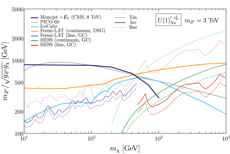
Figure 10: Combined limits from indirect detection, collider, and direct detection bounds on the $U(1)_{\text{ax}}^{\prime\,c_{V}^{t}}$ model with a 3 TeV mediator. For heavy DM, the anomaly-induced annihilations to gauge bosons lead to strong indirect detection bounds. Some of the indirect detection limits are sensitive to the halo profile, and for these the impact of choosing different halo profiles is shown.

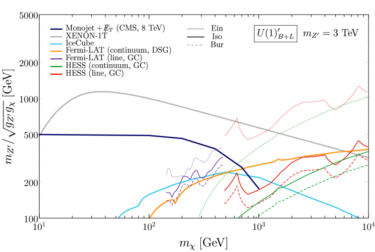
Figure 11: The same as in Fig. 10, shown for the $U(1)^{\prime}_{B+L}$ model.

Figure 12: The same as in Fig, 10, shown for the $U(1)^{\prime}_{L}$ model.

5 Comments on Validity of Our Results

Throughout our discussion, we have assumed that anomalies are canceled by fermions that are sufficiently decoupled so as to be effectively infinitely heavy for the processes that they mediate. Since the main effects of the Wess-Zumino terms are in DM annihilation, this corresponds to $m_{f}\gg m_{\chi}$. It is instructive to ask how our results change as the anomaly-canceling fermions are brought closer to the DM mass.

Let us illustrate this point with the particular example of DM annihilation in a $U(1)^{\prime}$ model where the charge of every SM fermion is equal to its usual hypercharge. Above the scale of the heaviest SM fermion, the top quark, there are no mixed $U(1)^{\prime}$-SM anomalies. Below the top mass, however, anomalies should appear and induce Wess-Zumino terms. At some point, where the DM becomes sufficiently lighter than the top mass, the EFT should give a good approximation to the full anomaly-free theory.

We compare these two calculation methods in Fig. 13, by varying the mass of the DM. The solid curve in Fig. 13 shows the annihilation cross section, calculated in the full UV complete theory, while the dashed line stands for the EFT calculation. By comparing the two curves, we see that the anomaly-canceling fermions can be treated as having infinite mass so long as they are at least 2-3 times heavier than the CM energy of the process being studied. In principle it is a very optimistic conclusion, that suggests that as long as the spectator fermions are not at the scale of the DM, our results are valid.

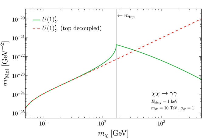
Figure 13: The effect of decoupling the top quark in a sequential hypercharge model. The green (solid) curve shows the cross section for DM annihilation to photons with $m_{t}=175$ GeV, while the red (dashed) curve shows the same cross section with an infinite top quark mass. In general, anomaly-induced effects rise with energy until the mass scale where the anomaly is resolved.

We also notice that in this particular example we have chosen the mass of the $Z^{\prime}$ to be very high, 10 TeV. Even though the top mass is much smaller than $m_{Z}^{\prime}$, the EFT is clearly valid in the case of light DM, showing again that the scale of the $Z^{\prime}$ plays no role in setting the validity range of the EFT.

6 Conclusions

Simplified models of DM are frequently used to present experimental results, yet the most common spin-1 mediator models often contain anomalies. While these may be resolved at high scales through the introduction of additional chiral fermions, in this work we have demonstrated that this is not without consequence. Integrating out heavy fermions generates Wess-Zumino terms, whose derivative couplings can create significant effects at high energies despite the loop suppression.

In particular, mixed anomalies cause couplings between the $Z^{\prime}$ and the SM gauge bosons. These interactions affect DM annihilation through the $Z^{\prime}$, and have the most impact on indirect detection probes of DM. We have evaluated the resulting bounds for a selection of $U(1)^{\prime}$ possibilities. The Wess-Zumino terms that we have computed depend only on the anomaly coefficients, and so DM annihilation cross sections to gauge bosons for an arbitrary $U(1)^{\prime}$ can in principle be obtained by scaling our results. If a new $U(1)$’ has vector couplings, the only anomaly-induced terms involve the $SU(2)_{L}$ bosons, and so the annihilation cross sections tend to be smaller. This leads to weaker constraints from indirect detection searches involving photons, under the assumption that the DM relic density is set by some external mechanism.

We have compared bounds from indirect detection with those from direct detection and colliders. We find that $\gamma$-ray searches can often provide the most stringent limits on heavy DM, with either continuum or line searches being more constraining depending on the choice of halo profile. For intermediate masses between a few hundred GeV and 1 TeV, IceCube can provide bounds comparable to direct searches if the scattering cross section with protons is SD. At small DM mass, direct detection is more effective at limiting a $Z^{\prime}$ which couples to quarks. Monojet and monophoton bounds can also constrain lighter DM, and while resonance searches are not directly comparable, dileptons still provide the best bounds if the mediator is kinematically accessible at the LHC and couples to quarks.

While most of our calculations assumed that the fermions which cancel anomalies are completely decoupled, we also considered the effect of restoring gauge invariance at smaller scales. As long as the anomalies persist up to energies that are a few times higher than the DM mass, which is the relevant energy scale for annihilation, our results remain completely valid.

In our study we have assumed that DM is a Majorana fermion, in part to emphasize our new indirect detection limits over the usual direct detection bounds, which are strong for spin-independent interactions that arise when the DM and quarks both couple vectorially to the $Z^{\prime}$. It would nevertheless be interesting to examine the interplay between direct and indirect detection bounds in more general models. For instance, if the DM is a Dirac fermion with a vector $U(1)^{\prime}$ coupling but the SM quarks couple axially under $U(1)^{\prime}$, the leading spin-independent direct detection interaction is velocity-suppressed. Dressing such an interaction with Higgses yields a pure vector interaction, but as the main effect involves a top loop, it can be avoided if the top does not couple to the $Z^{\prime}$. On the other hand, if the top does carry $U(1)^{\prime}$ charge but the light quarks do not, the $SU(3)_{C}^{2}\times U(1)^{\prime}$ anomaly could be relevant for collider searches as there is no tree-level DM production from light quark initial states.

In characterizing the sensitivities of DM searches, models that are employed to show experimental results should be consistent with theoretical considerations. In addition to the recently well-studied requirement that such models provide unitary scattering amplitudes, we have shown here how gauge invariance necessitates the inclusion of additional interactions beyond the minimal Lagrangian of generic simplified DM models. We look forward to future developments in this direction as searches for DM continue.

Appendix A Effective triple gauge boson couplings

Equation 4.1 gives the effective $Z^{\prime}$-$\gamma$-$\gamma$ vertex. Here, we provide the form of this vertex for other gauge boson channels.

The calculation of the $Z^{\prime}$-$g$-$g$ vertex is the same as for $Z^{\prime}$-$\gamma$-$\gamma$ up to a color factor and coupling constants:

$$\Gamma_{gg}^{\mu\nu\rho}=2\left(\frac{g_{s}}{eQ_{f}^{em}N_{c}}\right)^{2}\Gamma^{\mu\nu\rho}$$ (22)

For massive gauge bosons, we include the Goldstone amplitude in the Ward identities, as described in Sec. 2. Unlike the photon and gluon cases, a triangle vertex arises even if the $U(1)^{\prime}$ coupling of the loop fermion is vector-like, because the weak interactions violate parity. Similarly to the $Z^{\prime}$ coupling to fermions, we write the $Z$-fermion-fermion vertex as $i\frac{g_{w}}{c_{w}}\gamma^{\rho}(g_{V}^{Z}+g_{A}^{Z}\gamma^{5})$. Then, the $Z^{\prime}$-$Z$-$\gamma$ vertex is given by

$$\Gamma^{\mu\nu\rho}_{Z\gamma} = \frac{g_{Z^{\prime}}N_{c}^{2}g_{w}eQ_{f}^{em}(g_{V}g_{A}^{Z}+g_{A}g_{V}^{Z})}{\pi^{2}c_{w}}\Big{(}I_{1}^{Z\gamma}\epsilon^{\alpha\nu\rho\mu}(p_{2})_{\alpha}+I_{2}^{Z\gamma}\epsilon^{\alpha\nu\rho\mu}(p_{3})_{\alpha}$$

$$\ +I_{3}^{Z\gamma}\epsilon^{\alpha\beta\nu\mu}(p_{2})^{\rho}(p_{2})_{\alpha}(p_{3})_{\beta}+I_{4}^{Z\gamma}\epsilon^{\alpha\beta\nu\mu}(p_{3})^{\rho}(p_{2})_{\alpha}(p_{3})_{\beta}$$

$$\ +I_{5}^{Z\gamma}\epsilon^{\alpha\beta\rho\mu}(p_{2})^{\sigma}(p_{2})_{\alpha}(p_{3})_{\beta}+I_{6}^{Z\gamma}\epsilon^{\alpha\beta\rho\mu}(p_{3})^{\sigma}(p_{2})_{\alpha}(p_{3})_{\beta}\Big{)}$$

where the form factors, in terms of those in Eq. 4.1, are

$$I_{1}^{Z\gamma}(p_{2},p_{3};m_{f}) = (p_{2}\cdot p_{3})I_{3}^{Z\gamma}(p_{2},p_{3};m_{f})+p_{3}^{2}I_{4}^{Z\gamma}(p_{2},p_{3};m_{f})$$

$$I_{2}^{Z\gamma}(p_{2},p_{3};m_{f}) = p_{2}^{2}I_{5}^{Z\gamma}(p_{2},p_{3};m_{f})+(p_{2}\cdot p_{3})I_{6}^{Z\gamma}(p_{2},p_{3};m_{f})$$

$$\ -\frac{g_{V}g_{A}^{Z}}{g_{V}g_{A}^{Z}+g_{A}g_{V}^{Z}}m_{f}^{2}C_{0}(p_{3}^{2},p_{1}^{2},p_{2}^{2},m_{f}^{2},m_{f}^{2},m_{f}^{2})$$

$$I_{3}^{Z\gamma}(p_{2},p_{3};m_{f}) = -I_{3}(p_{2},p_{3};m_{f})$$ (24)

$$I_{4}^{Z\gamma}(p_{2},p_{3};m_{f}) = -I_{4}(p_{2},p_{3};m_{f})$$

$$I_{5}^{Z\gamma}(p_{2},p_{3};m_{f}) = -I_{5}(p_{2},p_{3};m_{f})$$

$$I_{6}^{Z\gamma}(p_{2},p_{3};m_{f}) = -I_{6}(p_{2},p_{3};m_{f})$$

The $Z^{\prime}$-$Z$-$Z$ vertex is

$$\Gamma^{\mu\nu\rho}_{ZZ} = \frac{g_{Z^{\prime}}N_{c}^{2}g_{w}^{2}(2g_{V}g_{V}^{Z}g_{A}^{Z}+g_{A}((g_{V}^{Z})^{2}+(g_{A}^{Z})^{2}))}{\pi^{2}c_{w}^{2}}\Big{(}I_{1}^{ZZ}\epsilon^{\alpha\nu\rho\mu}(p_{2})_{\alpha}+I_{2}^{ZZ}\epsilon^{\alpha\nu\rho\mu}(p_{3})_{\alpha}$$

$$\ +I_{3}^{ZZ}\epsilon^{\alpha\beta\nu\mu}(p_{2})^{\rho}(p_{2})_{\alpha}(p_{3})_{\beta}+I_{4}^{ZZ}\epsilon^{\alpha\beta\nu\mu}(p_{3})^{\rho}(p_{2})_{\alpha}(p_{3})_{\beta}$$

$$\ +I_{5}^{ZZ}\epsilon^{\alpha\beta\rho\mu}(p_{2})^{\sigma}(p_{2})_{\alpha}(p_{3})_{\beta}+I_{6}^{ZZ}\epsilon^{\alpha\beta\rho\mu}(p_{3})^{\sigma}(p_{2})_{\alpha}(p_{3})_{\beta}\Big{)}$$

where the form factors are

$$I_{1}^{ZZ}(p_{2},p_{3};m_{f}) = (p_{2}\cdot p_{3})I_{3}^{ZZ}(p_{2},p_{3};m_{f})+p_{3}^{2}I_{4}^{ZZ}(p_{2},p_{3};m_{f})-m_{f}^{2}C_{0}(p_{3}^{2},p_{1}^{2},p_{2}^{2},m_{f}^{2},m_{f}^{2},m_{f}^{2})$$

$$I_{2}^{ZZ}(p_{2},p_{3};m_{f}) = p_{2}^{2}I_{5}^{ZZ}(p_{2},p_{3};m_{f})+(p_{2}\cdot p_{3})I_{6}^{ZZ}(p_{2},p_{3};m_{f})-m_{f}^{2}C_{0}(p_{3}^{2},p_{1}^{2},p_{2}^{2},m_{f}^{2},m_{f}^{2},m_{f}^{2})$$

$$I_{3}^{ZZ}(p_{2},p_{3};m_{f}) = -I_{3}(p_{2},p_{3};m_{f})$$ (26)

$$I_{4}^{ZZ}(p_{2},p_{3};m_{f}) = -I_{4}(p_{2},p_{3};m_{f})$$

$$I_{5}^{ZZ}(p_{2},p_{3};m_{f}) = -I_{5}(p_{2},p_{3};m_{f})$$

$$I_{6}^{ZZ}(p_{2},p_{3};m_{f}) = -I_{6}(p_{2},p_{3};m_{f})$$

For the $Z^{\prime}$-$W^{+}$-$W^{-}$ vertex, we assume that two fermions run in the loop whose left-handed components are related by $SU(2)_{L}$, with the up-type fermion having mass $m_{f}$ and coupling vectorially to the $Z^{\prime}$, $-ig_{Z^{\prime}}\gamma^{\nu}$. Then, regardless of whether the down-type fermion coupling to the $Z^{\prime}$ is vector or axial, i.e. $-ig_{Z^{\prime}}\gamma^{\nu}$ or $ig_{Z^{\prime}}\gamma^{\nu}\gamma^{5}$, the vertex is given by

$$\Gamma^{\mu\nu\rho}_{WW} = \frac{g_{Z^{\prime}}N_{c}^{2}g_{w}^{2}}{4\pi^{2}}\Big{(}I_{1}^{WW}\epsilon^{\alpha\nu\rho\mu}(p_{2})_{\alpha}+I_{2}^{WW}\epsilon^{\alpha\nu\rho\mu}(p_{3})_{\alpha}$$

$$\ +I_{3}^{WW}\epsilon^{\alpha\beta\nu\mu}(p_{2})^{\rho}(p_{2})_{\alpha}(p_{3})_{\beta}+I_{4}^{WW}\epsilon^{\alpha\beta\nu\mu}(p_{3})^{\rho}(p_{2})_{\alpha}(p_{3})_{\beta}$$

$$\ +I_{5}^{WW}\epsilon^{\alpha\beta\rho\mu}(p_{2})^{\sigma}(p_{2})_{\alpha}(p_{3})_{\beta}+I_{6}^{WW}\epsilon^{\alpha\beta\rho\mu}(p_{3})^{\sigma}(p_{2})_{\alpha}(p_{3})_{\beta}\Big{)}$$

where the form factors are

$$I_{1}^{WW}(p_{2},p_{3};m_{f}) = (p_{2}\cdot p_{3})I_{3}^{WW}(p_{2},p_{3};m_{f})+p_{3}^{2}I_{4}^{WW}(p_{2},p_{3};m_{f})-\frac{m_{f}^{2}}{4}\Big{(}C_{0}(p_{3}^{2},p_{1}^{2},p_{2}^{2},m_{f}^{2},0,0)$$

$$\ +C_{1}(p_{3}^{2},p_{1}^{2},p_{2}^{2},m_{f}^{2},0,0)+C_{1}(p_{3}^{2},p_{1}^{2},p_{2}^{2},0,m_{f}^{2},m_{f}^{2})$$

$$\ +C_{2}(p_{3}^{2},p_{1}^{2},p_{2}^{2},m_{f}^{2},0,0)+C_{2}(p_{3}^{2},p_{1}^{2},p_{2}^{2},0,m_{f}^{2},m_{f}^{2})\Big{)}$$

$$I_{2}^{WW}(p_{2},p_{3};m_{f}) = p_{2}^{2}I_{5}^{WW}(p_{2},p_{3};m_{f})+(p_{2}\cdot p_{3})I_{6}^{WW}(p_{2},p_{3};m_{f})+\frac{m_{f}^{2}}{4}\Big{(}C_{0}(p_{3}^{2},p_{1}^{2},p_{2}^{2},m_{f}^{2},0,0)$$

$$\ +C_{1}(p_{3}^{2},p_{1}^{2},p_{2}^{2},m_{f}^{2},0,0)+C_{1}(p_{3}^{2},p_{1}^{2},p_{2}^{2},0,m_{f}^{2},m_{f}^{2})$$

$$\ +C_{2}(p_{3}^{2},p_{1}^{2},p_{2}^{2},m_{f}^{2},0,0)+C_{2}(p_{3}^{2},p_{1}^{2},p_{2}^{2},0,m_{f}^{2},m_{f}^{2})\Big{)}$$

$$I_{3}^{WW}(p_{2},p_{3};m_{f}) = \frac{1}{2}\left(C_{12}(p_{2}^{2},p_{1}^{2},p_{3}^{2},m_{f}^{2},0,0)+C_{12}(p_{2}^{2},p_{1}^{2},p_{3}^{2},0,m_{f}^{2},m_{f}^{2})\right)$$ (28)

$$I_{4}^{WW}(p_{2},p_{3};m_{f}) = -I_{5}^{WW}(p_{3},p_{2};m_{f})$$

$$I_{5}^{WW}(p_{2},p_{3};m_{f}) = \frac{1}{2}\Big{(}C_{11}(p_{2}^{2},p_{1}^{2},p_{3}^{2},m_{f}^{2},0,0)+C_{11}(p_{2}^{2},p_{1}^{2},p_{3}^{2},0,m_{f}^{2},m_{f}^{2})$$

$$\ +C_{1}(p_{2}^{2},p_{1}^{2},p_{3}^{2},m_{f}^{2},0,0)+C_{1}(p_{2}^{2},p_{1}^{2},p_{3}^{2},0,m_{f}^{2},m_{f}^{2})\Big{)}$$

$$I_{6}^{WW}(p_{2},p_{3};m_{f}) = -I_{3}^{WW}(p_{2},p_{3};m_{f})$$

Note added.

While this paper was being completed, related work Dror:2017ehi appeared which concentrates on the implications of anomalous $U(1)^{\prime}$ theories at low energies. The underlying physics is similar, but in contrast to the authors of Dror:2017ehi , we primarily consider theories of WIMP dark matter.

References

- (1) K. Griest and M. Kamionkowski, Unitarity Limits on the Mass and Radius of Dark Matter Particles, Phys. Rev. Lett. 64 (1990) 615.
- (2) G. Bertone, D. Hooper and J. Silk, Particle dark matter: Evidence, candidates and constraints, Phys. Rept. 405 (2005) 279–390, [hep-ph/0404175].
- (3) K. Petraki and R. R. Volkas, Review of asymmetric dark matter, Int. J. Mod. Phys. A28 (2013) 1330028, [1305.4939].
- (4) H. Baer, K.-Y. Choi, J. E. Kim and L. Roszkowski, Dark matter production in the early Universe: beyond the thermal WIMP paradigm, Phys. Rept. 555 (2015) 1–60, [1407.0017].
- (5) XENON collaboration, E. Aprile et al., First Dark Matter Search Results from the XENON1T Experiment, 1705.06655.
- (6) DES, Fermi-LAT collaboration, A. Drlica-Wagner et al., Search for Gamma-Ray Emission from DES Dwarf Spheroidal Galaxy Candidates with Fermi-LAT Data, Astrophys. J. 809 (2015) L4, [1503.02632].
- (7) Fermi-LAT collaboration, M. Ackermann et al., Searching for Dark Matter Annihilation from Milky Way Dwarf Spheroidal Galaxies with Six Years of Fermi Large Area Telescope Data, Phys. Rev. Lett. 115 (2015) 231301, [1503.02641].
- (8) H.E.S.S. collaboration, H. Abdallah et al., Search for dark matter annihilations towards the inner Galactic halo from 10 years of observations with H.E.S.S, Phys. Rev. Lett. 117 (2016) 111301, [1607.08142].
- (9) J. Goodman, M. Ibe, A. Rajaraman, W. Shepherd, T. M. P. Tait and H.-B. Yu, Constraints on Light Majorana dark Matter from Colliders, Phys. Lett. B695 (2011) 185–188, [1005.1286].
- (10) Y. Bai, P. J. Fox and R. Harnik, The Tevatron at the Frontier of Dark Matter Direct Detection, JHEP 12 (2010) 048, [1005.3797].
- (11) J. Goodman, M. Ibe, A. Rajaraman, W. Shepherd, T. M. P. Tait and H.-B. Yu, Constraints on Dark Matter from Colliders, Phys. Rev. D82 (2010) 116010, [1008.1783].
- (12) J. Fan, M. Reece and L.-T. Wang, Non-relativistic effective theory of dark matter direct detection, JCAP 1011 (2010) 042, [1008.1591].
- (13) A. L. Fitzpatrick, W. Haxton, E. Katz, N. Lubbers and Y. Xu, The Effective Field Theory of Dark Matter Direct Detection, JCAP 1302 (2013) 004, [1203.3542].
- (14) G. Busoni, A. De Simone, E. Morgante and A. Riotto, On the Validity of the Effective Field Theory for Dark Matter Searches at the LHC, Phys. Lett. B728 (2014) 412–421, [1307.2253].
- (15) O. Buchmueller, M. J. Dolan and C. McCabe, Beyond Effective Field Theory for Dark Matter Searches at the LHC, JHEP 01 (2014) 025, [1308.6799].
- (16) G. Busoni, A. De Simone, J. Gramling, E. Morgante and A. Riotto, On the Validity of the Effective Field Theory for Dark Matter Searches at the LHC, Part II: Complete Analysis for the -channel, JCAP 1406 (2014) 060, [1402.1275].
- (17) G. Busoni, A. De Simone, T. Jacques, E. Morgante and A. Riotto, On the Validity of the Effective Field Theory for Dark Matter Searches at the LHC Part III: Analysis for the -channel, JCAP 1409 (2014) 022, [1405.3101].
- (18) H. An, X. Ji and L.-T. Wang, Light Dark Matter and Dark Force at Colliders, JHEP 07 (2012) 182, [1202.2894].
- (19) M. T. Frandsen, F. Kahlhoefer, A. Preston, S. Sarkar and K. Schmidt-Hoberg, LHC and Tevatron Bounds on the Dark Matter Direct Detection Cross-Section for Vector Mediators, JHEP 07 (2012) 123, [1204.3839].
- (20) G. Arcadi, Y. Mambrini, M. H. G. Tytgat and B. Zaldivar, Invisible and dark matter: LHC vs LUX constraints, JHEP 03 (2014) 134, [1401.0221].
- (21) X. Chu, Y. Mambrini, J. Quevillon and B. Zaldivar, Thermal and non-thermal production of dark matter via Z’-portal(s), JCAP 1401 (2014) 034, [1306.4677].
- (22) E. Dudas, L. Heurtier, Y. Mambrini and B. Zaldivar, Extra U(1), effective operators, anomalies and dark matter, JHEP 11 (2013) 083, [1307.0005].
- (23) M. Fairbairn and J. Heal, Complementarity of dark matter searches at resonance, Phys. Rev. D90 (2014) 115019, [1406.3288].
- (24) O. Lebedev and Y. Mambrini, Axial dark matter: The case for an invisible , Phys. Lett. B734 (2014) 350–353, [1403.4837].
- (25) A. Alves, A. Berlin, S. Profumo and F. S. Queiroz, Dark Matter Complementarity and the Z′ Portal, Phys. Rev. D92 (2015) 083004, [1501.03490].
- (26) A. Alves, A. Berlin, S. Profumo and F. S. Queiroz, Dirac-fermionic dark matter in U(1)X models, JHEP 10 (2015) 076, [1506.06767].
- (27) F. Kahlhoefer, K. Schmidt-Hoberg, T. Schwetz and S. Vogl, Implications of unitarity and gauge invariance for simplified dark matter models, JHEP 02 (2016) 016, [1510.02110].
- (28) T. Jacques, A. Katz, E. Morgante, D. Racco, M. Rameez and A. Riotto, Complementarity of DM searches in a consistent simplified model: the case of , JHEP 10 (2016) 071, [1605.06513].
- (29) G. Busoni et al., Recommendations on presenting LHC searches for missing transverse energy signals using simplified -channel models of dark matter, 1603.04156.
- (30) A. Albert et al., Recommendations of the LHC Dark Matter Working Group: Comparing LHC searches for heavy mediators of dark matter production in visible and invisible decay channels, 1703.05703.
- (31) A. Ismail, W.-Y. Keung, K.-H. Tsao and J. Unwin, Axial vector and anomaly cancellation, Nucl. Phys. B918 (2017) 220–244, [1609.02188].
- (32) M. B. Green and J. H. Schwarz, Anomaly Cancellation in Supersymmetric D=10 Gauge Theory and Superstring Theory, Phys. Lett. B149 (1984) 117–122.
- (33) J. Ellis, M. Fairbairn and P. Tunney, Anomaly-Free Dark Matter Models are not so Simple, 1704.03850.
- (34) E. D’Hoker and E. Farhi, Decoupling a Fermion in the Standard Electroweak Theory, Nucl. Phys. B248 (1984) 77.
- (35) E. D’Hoker and E. Farhi, Decoupling a Fermion Whose Mass Is Generated by a Yukawa Coupling: The General Case, Nucl. Phys. B248 (1984) 59–76.
- (36) J. Preskill, Gauge anomalies in an effective field theory, Annals Phys. 210 (1991) 323–379.
- (37) Y. Mambrini, A Clear Dark Matter gamma ray line generated by the Green-Schwarz mechanism, JCAP 0912 (2009) 005, [0907.2918].
- (38) E. Dudas, Y. Mambrini, S. Pokorski and A. Romagnoni, (In)visible Z-prime and dark matter, JHEP 08 (2009) 014, [0904.1745].
- (39) F. Domingo, O. Lebedev, Y. Mambrini, J. Quevillon and A. Ringwald, More on the Hypercharge Portal into the Dark Sector, JHEP 09 (2013) 020, [1305.6815].
- (40) G. Arcadi, P. Ghosh, Y. Mambrini, M. Pierre and F. S. Queiroz, portal to Chern-Simons Dark Matter, 1706.04198.
- (41) A. Bilal, Lectures on Anomalies, 0802.0634.
- (42) J. Preskill, “Physics 230 notes.” http://www.theory.caltech.edu/~preskill/ph230/notes/230Chapter3-Page23-74.pdf, 1983.
- (43) P. Anastasopoulos, F. Fucito, A. Lionetto, G. Pradisi, A. Racioppi and Y. S. Stanev, Minimal Anomalous U(1)-prime Extension of the MSSM, Phys. Rev. D78 (2008) 085014, [0804.1156].
- (44) A. Racioppi, Anomalies, and the MSSM. PhD thesis, Rome U., Tor Vergata, 2009. 0907.1535.
- (45) E. D’Hoker and E. Farhi, Decoupling a Fermion Whose Mass Is Generated by a Yukawa Coupling: The General Case, Nucl. Phys. B248 (1984) 59–76.
- (46) E. D’Hoker and E. Farhi, Decoupling a Fermion in the Standard Electroweak Theory, Nucl. Phys. B248 (1984) 77.
- (47) J. Wess and B. Zumino, Consequences of anomalous Ward identities, Phys. Lett. B37 (1971) 95–97.
- (48) N. F. Bell, Y. Cai and R. K. Leane, Impact of mass generation for spin-1 mediator simplified models, JCAP 1701 (2017) 039, [1610.03063].
- (49) Y. Cui and F. D’Eramo, On the Completeness of Vector Portal Theories: New Insights into the Dark Sector and its Interplay with Higgs Physics, 1705.03897.
- (50) J. Kopp, L. Michaels and J. Smirnov, Loopy Constraints on Leptophilic Dark Matter and Internal Bremsstrahlung, JCAP 1404 (2014) 022, [1401.6457].
- (51) J. Abdallah et al., Simplified Models for Dark Matter Searches at the LHC, Phys. Dark Univ. 9-10 (2015) 8–23, [1506.03116].
- (52) P. Artoisenet et al., A framework for Higgs characterisation, JHEP 11 (2013) 043, [1306.6464].
- (53) C. Garcia-Cely and A. Rivera, General calculation of the cross section for dark matter annihilations into two photons, JCAP 1703 (2017) 054, [1611.08029].
- (54) L. Rosenberg, Electromagnetic interactions of neutrinos, Phys. Rev. 129 (1963) 2786–2788.
- (55) T. Hahn and M. Perez-Victoria, Automatized one loop calculations in four-dimensions and D-dimensions, Comput. Phys. Commun. 118 (1999) 153–165, [hep-ph/9807565].
- (56) G. Arcadi, M. Dutra, P. Ghosh, M. Lindner, Y. Mambrini, M. Pierre et al., The Waning of the WIMP? A Review of Models, Searches, and Constraints, 1703.07364.
- (57) M. Cirelli, G. Corcella, A. Hektor, G. Hutsi, M. Kadastik, P. Panci et al., PPPC 4 DM ID: A Poor Particle Physicist Cookbook for Dark Matter Indirect Detection, JCAP 1103 (2011) 051, [1012.4515].
- (58) Fermi-LAT collaboration, M. Ackermann et al., Updated search for spectral lines from Galactic dark matter interactions with pass 8 data from the Fermi Large Area Telescope, Phys. Rev. D91 (2015) 122002, [1506.00013].
- (59) H.E.S.S. collaboration, A. Abramowski et al., Search for Photon-Linelike Signatures from Dark Matter Annihilations with H.E.S.S., Phys. Rev. Lett. 110 (2013) 041301, [1301.1173].
- (60) M. Lisanti, Lectures on Dark Matter Physics, in Proceedings, Theoretical Advanced Study Institute in Elementary Particle Physics: New Frontiers in Fields and Strings (TASI 2015): Boulder, CO, USA, June 1-26, 2015, pp. 399–446, 2017. 1603.03797. DOI.
- (61) IceCube collaboration, M. G. Aartsen et al., Search for annihilating dark matter in the Sun with 3 years of IceCube data, Eur. Phys. J. C77 (2017) 146, [1612.05949].
- (62) M. Cirelli, E. Del Nobile and P. Panci, Tools for model-independent bounds in direct dark matter searches, JCAP 1310 (2013) 019, [1307.5955].
- (63) R. Catena and B. Schwabe, Form factors for dark matter capture by the Sun in effective theories, JCAP 1504 (2015) 042, [1501.03729].
- (64) CMS collaboration, V. Khachatryan et al., Search for narrow resonances in dilepton mass spectra in proton-proton collisions at = 13 TeV and combination with 8 TeV data, Phys. Lett. B768 (2017) 57–80, [1609.05391].
- (65) CMS collaboration, V. Khachatryan et al., Search for dark matter, extra dimensions, and unparticles in monojet events in proton–proton collisions at TeV, Eur. Phys. J. C75 (2015) 235, [1408.3583].
- (66) P. J. Fox, R. Harnik, J. Kopp and Y. Tsai, LEP Shines Light on Dark Matter, Phys. Rev. D84 (2011) 014028, [1103.0240].
- (67) DELPHI collaboration, J. Abdallah et al., Photon events with missing energy in e+ e- collisions at s**(1/2) = 130-GeV to 209-GeV, Eur. Phys. J. C38 (2005) 395–411, [hep-ex/0406019].
- (68) DELPHI collaboration, J. Abdallah et al., Search for one large extra dimension with the DELPHI detector at LEP, Eur. Phys. J. C60 (2009) 17–23, [0901.4486].
- (69) U. Haisch and F. Kahlhoefer, On the importance of loop-induced spin-independent interactions for dark matter direct detection, JCAP 1304 (2013) 050, [1302.4454].
- (70) PICO collaboration, C. Amole et al., Dark Matter Search Results from the PICO-60 C3F8 Bubble Chamber, 1702.07666.
- (71) A. L. Fitzpatrick, W. Haxton, E. Katz, N. Lubbers and Y. Xu, Model Independent Direct Detection Analyses, 1211.2818.
- (72) N. Anand, A. L. Fitzpatrick and W. C. Haxton, Weakly interacting massive particle-nucleus elastic scattering response, Phys. Rev. C89 (2014) 065501, [1308.6288].
- (73) J. A. Dror, R. Lasenby and M. Pospelov, New constraints on light vectors coupled to anomalous currents, 1705.06726.