Direct verification of the fluctuation-dissipation relation in viscously coupled oscillators

Abstract

The fluctuation-dissipation relation, a central result in non-equilibrium statistical physics, relates equilibrium fluctuations in a system to its linear response to external forces. Here we provide a direct experimental verification of this relation for viscously coupled oscillators, as realized by a pair of optically trapped colloidal particles. A theoretical analysis, in which interactions mediated by slow viscous flow are represented by non-local friction tensors, matches experimental results and reveals a frequency maximum in the amplitude of the mutual response which is a sensitive function of the trap stiffnesses and the friction tensors. This allows for its location and width to be tuned and suggests the utility of the trap setup for accurate two-point microrheology.

The relation between the generalized susceptibility and equilibrium fluctuations of the generalized forces, first obtained for a linear resistive circuit by Nyquist Nyquist (1928) and then proved for any general linear dissipative system by Callen and Welton Callen and Welton (1951), is a central result in non-equilibrium statistical physics. The relation can be used to infer the intrinsic fluctuations of a system from measurements of its response to external perturbations or, perhaps more startlingly, to predict its response to external perturbations from the character of its intrinsic fluctuations Kubo (1966). The fluctuation-dissipation relation is the point of departure for several areas of current research including fluctuation relations Seifert (2012), relaxation in glasses Berthier and Biroli (2011), and response and correlations in active Fodor et al. (2016) and driven systems Mason and Weitz (1995); Levine and Lubensky (2000).

The first experimental verification of the relation between fluctuation and dissipation was due to Johnson Johnson (1928), whose investigation of the “thermal agitation of electricity in conductors” provided the motivation for Nyquist’s theoretical work Nyquist (1928). Though the relation has been verified since in systems with conservative couplings, a direct verification in a system where the coupling is entirely dissipative is, to the best of our knowledge, not available. Colloidal particles in a viscous fluid interact through velocity-dependent many-body hydrodynamic forces whose strength, away from boundaries, is inversely proportional to the distance between the particles. The range of these dissipative forces can be made much greater than that of conservative forces such as the DLVO interaction Derjaguin and Landau (1941); Verwey and Overbeek (1948). Therefore, it is possible to engineer a situation where the dominant coupling between colloidal particles is the viscous hydrodynamic force and all other interactions are negligibly small. Such systems, then, are ideal for testing the fluctuation-dissipation relation when couplings are purely dissipative.

In this Letter, we present a direct verification of the fluctuation-dissipation relation for a pair of optically trapped colloidal particles in water. We measure the equilibrium fluctuations of the distance between the particles and the response of one particle to the sinusoidal motion of another particle. Transforming both correlations and responses to the frequency domain, we verify the fluctuation-dissipation relation over a range of frequencies spanning two orders of magnitude. Remarkably, the response function has a peak in frequency, reminiscent of a resonance, though the system of oscillators is entirely overdamped. A theoretical analysis, assuming slow viscous flow of the ambient water, is in excellent agreement with the experiments. The analysis reveals that the location and width of the resonant peak can be tuned by altering the viscosity, the separation between the particles, the trap stiffnesses, and the colloidal diameters. It provides the inverse relations necessary for using the trap setup for accurate two-point microrheology. We now present details of our experiment and its analysis.

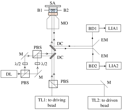
Figure 1: A schematic diagram of the experimental setup. TL1: trapping laser for driving particle B1, TL2: trapping laser for driven particle B2, DL: detection laser, PBS: polarizing beam splitter cube, $\frac{\lambda}{2}$: half wave plate, DC: dichroic mirror, MO: microscope objective, CS: cover slip, BD1 and BD2: balanced detection systems based on Thorlabs photodiodes PD-EC2, M: mirror, EM: edge mirror, LIA1 and LIA2: lock-in amplifiers for B1 and B2, respectively.

Experiment: The details of the experimental setup towards validation of the fluctuation-dissipation theorem are provided in Supplementary Information - here we provide a brief description. Thus, we set up a dual-beam optical tweezers (Fig.1) by focusing two orthogonally polarized beams of wavelength $\lambda=1064$ nm generated independently from two diode lasers using a high NA immersion-oil microscope objective (Zeiss PlanApo,$100\times 1.4$). One of the lasers is modulated using an AOM located conjugate to the back-focal plane of the microscope objective, and a long optical path after the AOM ensures that a minimal beam deflection is enough to modulate one of the trapped beams, so that the intensity in the first order remains constant to around 2%. The modulated and unmodulated beams are independently coupled into the trapping microscope using mirrors and a polarizing beam splitter, while detection is performed using a separate laser at 671 nm generating two detection beams also orthogonally polarized and superposed on the respective trapping beams using dichroic beam splitters. The two trapped beads are imaged and their displacements measured by back-focal- plane-interferometry, with the imaging white light and detection beams also separated at the output by dichroic beam splitters, which along with the orthogonal polarization scheme ensures that cross-talk in the detection beams is absent. A very low volume fraction sample ($\phi\approx 0.01$) is prepared with 3 $\mu$m diameter polystyrene latex beads in 1 M NaCl-water solution for avoiding surface charges. We trap two spherical polystyrene beads (Sigma LB-30) of mean size 3 $\mu$m each, in two calibrated optical traps which are separated by a distance $4\pm 0.1\>\mu$m, so that the surface-surface distance of the trapped beads is $1\pm 0.2\>\mu$m ($0.67a$, $a$ being the particle radius) and the distance from the cover slip surface is 30 $\mu$m ($20a$, so as to overrule wall effects). From the literature Stilgoe et al. (2011), the particle separation is still large enough to avoid effects due to optical binding and surface charges. In order to ensure that the trapping and detection beams are not influencing each other, we measure the Brownian motion of a trapped particle when the trapping and detection beams for the other trap is switched on (in the absence of a particle), and check that there are no changes in the measured trap stiffness. One of the traps is sinusoidally modulated (amplitude around $0.2a$) and the phase and amplitude response of both the driving and driven particles with reference to the sinusoidal drive are measured by lock-in detection (Stanford Research, SR830). To get large signal to noise, we use balanced detection systems BD1 and BD2, for the driving and driven particles, respectively. The voltage-amplitude calibration of our detection system reveals that we can resolve motion of around 5 nm with an SNR of 2.

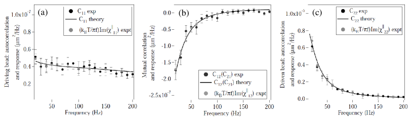
Figure 2: Verification of the fluctuation-dissipation relation $C_{ij}=(k_{B}T/\pi f)\,\text{Im}(\chi_{ij}^{\parallel})$ for a pair of viscously coupled colloidal particles in optical traps. The first and third panels compare the self-response and the position auto-correlation of, respectively, the driving and driven colloid, while the second panel compares their mutual-response and cross-correlation. Theoretically computed correlation functions, assuming over-damped motion of the colloids and slow viscous flow in the fluid, are shown as solid lines.

Each of the optical traps are calibrated using equipartition and power spectrum methods considering the particle temperature to be same as the room temperature. We verify that each of the potentials is harmonic in nature from the histogram of the Brownian motion which is satisfactorily Gaussian (Fig.A.1 in Supplementary Information), even when both trapping beams are on. The sampling frequency is 2 kHz, while we performed data blocking at the level of 100 points in order to ensure good Lorentzian fits Berg-Sørensen and Flyvbjerg (2004) for trap calibration. We maintain a considerably higher stiffness for the particle in the modulated trap so that it is not affected by the back-flow due to the driven particle. The low stiffness of the driven trap ensures that it has a maximal response to the drive. Thus, for validation of the fluctuation-dissipation theorem, the stiffness of the modulated bead (B1) was 69.6 $\mu N/m$, while that of the driven is 4.8 $\mu N/m$. Note that, to observe a clear amplitude resonance, a lower ratio of trap stiffness is required, as we demonstrate later. The verification of the fluctuation-dissipation theorem is shown in Fig.2. It is understandable that while the fluctuation-dissipation theorem is in the form a simple equation for a single particle, for two particles the equations would be represented in the form of a matrix, which we discuss in more detail later. This is what we demonstrate in Fig.2(a), (b), and (c), where the auto and cross-correlations for both particles are matched with the corresponding response functions. The auto-correlation function of B1 is shown in Fig.2(a), while that of B2 is shown in Fig.2(b). The corresponding response functions ($\mathit{\chi_{11}^{||},\>\chi{}_{22}^{||}}$) are obtained by measuring the amplitude and phase of the individual particles when they are themselves driven. Fig.2(c) shows the cross-correlation function which is again compared with the corresponding response function $\mathit{\chi_{12}^{||}}$. This is obtained by measuring the amplitude and phase of B2 when B1 is driven. Note that we are not able to measure $\mathit{\chi_{21}^{||}}$which is the response of B1 when B2 is driven since the much larger stiffness of B1 renders the amplitude of the response extremely small so that it is beyond our detection sensitivity. For the response measurements, each data point is the average of ten separate measurements at each frequency. It is clear from the figures that we obtain a good match between fluctuation and response - which essentially validates the fluctuation-dissipation relations for a pair of colloidal particles coupled by hydrodynamic interactions. Note that for consistency check, we also plot the cross-correlation function in the time domain (Fig.A.4 in Supplementary Information) and obtain qualitatively similar data as reported in Ref. Meiners and Quake (1999).

Theory: The Langevin equations describing the stochastic trajectories of the colloids are Gardiner (1985)

$$m_{i}\dot{\boldsymbol{v}_{i}} +\boldsymbol{\gamma}_{ij}\cdot\boldsymbol{v}_{j}+{\bf\boldsymbol{\nabla}}_{i}U=\boldsymbol{{\bf\xi}}_{i},$$ (1)

where $i,j=1,2$ refer to the driving and driven colloid, $m_{i}$ are their masses, $\boldsymbol{v}_{i}$ are their velocities, $\boldsymbol{\gamma}_{ij}$ are the second-rank friction tensors encoding the velocity-dependent dissipative forces mediated by the fluid, $U=U_{1}+U_{2}$ is the total potential of the conservative forces, and $\boldsymbol{\xi}_{i}$, the Langevin noises, are zero-mean Gaussian random variables whose variance is provided by the fluctuation-dissipation relation $\langle\boldsymbol{\xi}_{i}(t)\boldsymbol{\xi}_{j}(t^{\prime})\rangle=2k_{B}T\boldsymbol{\gamma}_{ij}\delta(t-t^{\prime})$. The bold-face notation, with Cartesian indices suppressed, is used for both vectors and tensors.

In the limit of slow viscous flow in the fluid, the friction tensors can be calculated from the Stokes equation using a variety of methods Ladd (1988); Mazur and Saarloos (1982); Cichocki et al. (1994); Singh and Adhikari (2016a, b). To leading order the result is

$$\boldsymbol{\gamma}_{ij}=\delta_{ij}\boldsymbol{I}\gamma_{i}-(1-\delta_{ij})\gamma_{i}\gamma_{j}\mathcal{F}_{i}\mathcal{F}_{j}\boldsymbol{G}(\boldsymbol{r}_{i},\boldsymbol{r}_{j}),$$ (2)

where $\gamma_{i}=6\pi\eta a_{i}$ are the self-frictions, $\boldsymbol{G}$ is a Green’s function of the Stokes equation Pozrikidis (1992), $\boldsymbol{r}_{i}$ are the centers of the colloids and $\mathcal{F}_{i}=1+\frac{a_{i}^{2}}{6}\nabla_{i}^{2}$ are the Faxén corrections that account for the finite radius, $a_{i}$, of the colloids. We emphasize that this expression is not limited to the translationally invariant Green’s function of unbounded flow, $8\pi\eta\,\boldsymbol{G}(\boldsymbol{r})=(\nabla^{2}\boldsymbol{I}-\boldsymbol{\nabla\nabla})r$, but holds generally for any Green’s function and is both symmetric and positive-definite Singh and Adhikari (2016a, b). The mutual friction tensors decay inversely with distance in an unbounded fluid and more rapidly in the proximity of boundaries. The assumption of slow viscous flow is valid at frequencies $\omega\tau_{\nu}\ll 1$ where $\tau_{\nu}=\rho L^{2}/\eta$ is the vorticity diffusion time scale Kim and Karrila (1992).

The harmonic optical potentials are given by $U_{i}(t)=\frac{1}{2}k_{i}|{\bf\boldsymbol{r}}_{i}-{\bf\boldsymbol{r}}_{i}^{0}|^{2}$ where $\boldsymbol{r}_{i}^{0}$ are the centers and $k_{i}$ are the stiffnesses of the optical traps. Note the absence of conservative mutual couplings. The system remains in equilibrium when the trap centers are stationary but is driven into non-equilibrium when they are modulated in time as $\boldsymbol{r}_{i}^{0}(t)$. For small modulations the response is linear.

For modulation frequencies $\omega\ll\gamma_{i}/m_{i}$ the velocities can be adiabatically eliminated from the inertial Langevin equations to yield inertialess Langevin equations for the positions Gardiner (1984). The multiplicative noises in the resulting equations have clear interpretations within the adiabatic elimination procedure; there is no Itô-Stratonovich dilemma van Kampen (1981); Gardiner (1985); van Kampen (1992); Klimontovich (1990, 1994). Both correlation and response functions can be calculated in this limit. Linearizing about the mean separation between the trap centers and decomposing the motion into components parallel and perpendicular to the separation vector, the result for the parallel response function is

$$\text{Im}\left[\chi_{ij}^{||}(\omega)\right]=\frac{\omega M_{ij}}{(\text{det}A-\omega^{2})^{2}+(\omega\begin{tabular}[]{c}tr\end{tabular}A)^{2}},$$ (4)

where $A_{ij}=\mu_{ij}^{||}k_{j}$ is a “response” matrix, the mobility matrix $\mu_{ij}^{||}$ is the inverse of the friction matrix and

$$M_{ij}=\left(\begin{array}[]{cc}\begin{tabular}[]{c}$\tfrac{k_{2}}{k_{1}}\mu_{22}^{\parallel}$\end{tabular}\text{det}A+\mu_{11}^{\parallel}\omega^{2}&-\mu_{12}^{\parallel}(\text{det}A-\omega^{2})\\ &\\ -\mu_{21}^{\parallel}(\text{det}A-\omega^{2})&\begin{tabular}[]{c}$\tfrac{k_{1}}{k_{2}}\mu_{11}^{\parallel}$\end{tabular}\text{det}A+\mu_{22}^{\parallel}\omega^{2}\end{array}\right).$$

The magnitude of the response of the driven bead to the driving bead is maximum at the “resonance” frequency

$$\omega_{res}=\sqrt{\text{det}A}=\sqrt{\mu_{11}^{\parallel}\mu_{22}^{\parallel}k_{1}k_{2}\left(1-\frac{\mu_{12}^{\parallel}\mu_{21}^{\parallel}}{\mu_{11}^{\parallel}\mu_{22}^{\parallel}}\right)}.$$ (5)

A simple analysis of the system with the two particles executing Brownian motion in the absence of the external drive leads us to write down the auto and cross-correlation functions ($C_{ij}$), so that by comparing with the response functions $\text{Im}(\chi_{ij}^{\parallel})$, we have $C_{ij}=(k_{B}T/\pi f)\,\text{Im}(\chi_{ij}^{\parallel})$ which is the well known fluctuation-dissipation relationship Kubo (1966).

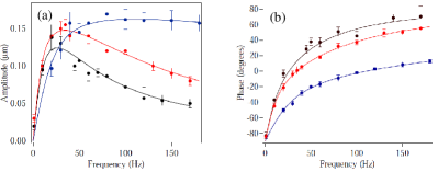
Figure 3: Amplitude and phase response for driven (B2) bead for different trap stiffness ratios with the inter-particle separation $0.67a$. (a) and (b) demonstrate amplitude and phase responses (with respect to driving frequency) of B2, for trap stiffness ratios of 2.5:1 (black), 5.7:1 (red), and 14.5:1 (blue). The resonance frequency in (a) is 20 Hz (black), 35 Hz (red), and 111 Hz (blue). The solid spheres denote experimental data points while the solid lines are corresponding theoretical fits.

This is indeed what we validate in Fig.2(a)-(c).

We now focus on a particularly interesting facet of our problem, namely the amplitude and phase response of B2 under the influence of the driven particle B1. We study this experimentally for three different trap stiffness ratios of B1 and B2, the results of which are shown in Fig.3(a) and (b). Note that we fit each graph with the calculated values of the responses for the experimental parameters used, and obtain very good fits. The amplitude and phase response of B1 (Supplementary information) to the drive frequency is expected, with the amplitude decaying with increasing frequency, and the phase being in sync with the drive at low frequencies and gradually lagging behind as the frequency is increased. However, the amplitude response of B2 is rather interesting, and shows a clear resonance response at a certain frequency, the value of which increases as the stiffness ratio of the traps is increased - it being dependent on the product of the stiffnesses as is clear from Eq.5. Thus, we have a resonance frequency of around 111 Hz (blue solid spheres in Fig.3(a)) with $\mathit{k_{1}:k_{2}}=$14.5:1, a frequency of around 33 Hz with a ratio of 5.7:1 (red solid spheres), and a frequency of around 20 Hz with a ratio of 2.5:1 (black solid spheres). In fact, it is as if the entrained fluid has minimum impedance around this frequency, so that there is maximum energy transfer between the driving and the driven beads. The amplitude of the resonance has an inverse dependence on the particle separation, so that with our current detection sensitivity, we do not observe the resonance effects beyond a surface-surface separation greater than $3a$. However, even this increased distance is also smaller than that used in earlier experiments, which possibly explains the fact that this phenomenon has not been reported earlier. The width of the resonance ($\mathit{Q}$ factor) is also dependent on the stiffness ratio, and increases as the latter is reduced. For a given medium, the resonance can thus be tuned by changing the stiffness ratios (as well as the inter-particle separation and particle diameters). Interestingly, it is obvious that the value of the $\mathit{Q}$-factor as well as the resonance frequency also depends on the damping, and can be modified by changing the viscosity of the solution. This property promises the measurement of this frequency shift as an accurate two-point micro-rheology probe of local viscosity of a fluid. Finally, the phase response in 3(b) is easily explained: B2 lags 90 degrees in phase with respect to the drive at very low frequencies with the lag reducing until the drive and driven are in phase at resonance, after which the driven bead leads in phase, and asymptotically approaches 90 degrees at high frequencies. The rate of approach is also determined by the stiffness ratio, and is rather slow at large stiffness ratios. Indeed, this is exactly similar to the relationship between velocity and driving force for a forced damped harmonic oscillator, and arises due to the fact that the oscillators are dissipatively coupled.

In conclusion, we perform a direct experimental verification of the fluctuation-dissipation relation in a system consisting of two colloidal particles confined in a viscous medium (water) in very close proximity (surface-surface separation less than the particle radius) using separate optical tweezers. Our results provide a confirmation of the validity of the fluctuation-dissipation relation in the presence of long-ranged dissipative forces that are the only source of coupling of, otherwise, independent degrees of freedom. Surprisingly, we identify a resonance in the response in a system which is overdamped and suggest its use in accurate two-point microrheology. The present experiment can be extended in several directions: measurements at higher frequencies can uncover the effects of retarded hydrodynamic interactions and the role of particle inertia while holographic traps can be used to test the fluctuation-dissipation relation in the presence of many-body hydrodynamic interactions. Some of these will be presented in forthcoming work.

This work was supported by the Indian Institute of Science Education and Research, Kolkata, an autonomous research and teaching institute funded by the Ministry of Human Resource Development, Govt. of India. We acknowledge computing resources on the Annapurna cluster provided by The Institute of Mathematical Sciences.

Supplemental information

Appendix A Experiment

We set up a dual-beam optical tweezers (Fig.A.1) by focusing two orthogonally polarized beams of wavelength $\lambda=1064$ nm generated independently from two diode lasers using a high NA immersion-oil microscope objective (Zeiss PlanApo,$100\times 1.4$). An AOM, located conjugate to the back-focal plane of the objective using the telescopic lens pair L1-L2 (see Fig.A.1), is used for modulating one of the traps. A long optical path after the AOM ensures that a minimal beam deflection is enough to modulate one of the trapped beams, so that the intensity in the first order remains constant to around 2%. The modulated and unmodulated beams are independently steered using mirror pairs M1, M2 and M3, M4, respectively, and coupled into a polarizing beam splitter (PBS1). For detection, we use a separate laser of wavelength $\lambda=671$ nm, that is again divided into two beams of orthogonal polarization by PBS2 and coupled into PBS3. We then use a dichroic (DC1) to overlap the two pairs of trapping and detection beams into the optical tweezers microscope (Zeiss Axiovert.A1). The two trapped beads are imaged and their displacements measured by back-focal- plane-interferometry, while the white light for imaging and the detection laser beams are separated by dichroics DC2 and DC3, respectively. A very low volume fraction sample ($\phi\approx 0.01$) is prepared with 3 $\mu$m diameter polystyrene latex beads in 1 M NaCl-water solution for avoiding surface charges. A single droplet of about 20 $\mu$l volume of the sample is introduced in a sample chamber made out of a standard 10 mm square cover slip attached by double-sided sticky tape to a microscope slide. We trap two spherical polystyrene beads (Sigma LB-30) of mean size 3 $\mu$m each, in two calibrated optical traps which are separated by a distance $4\pm 0.1\>\mu$m, so that the surface-surface distance of the trapped beads is $1\pm 0.2\>\mu$m, and the distance from the cover slip surface is 30 $\mu$m. From the literature, this distance is still large enough to avoid optical cross talk and effects due to surface charges Stilgoe et al. (2011). In order to ensure that the trapping beams do not influence each other, we measure the Brownian motion of one when the other is switched on (in the absence of a particle), and check that there are no changes in the Brownian motion. One of the traps is sinusoidally modulated and the phase and amplitude response of both the driving and driven particles with reference to the sinusoidal drive are measured by lock-in detection (Stanford Research, SR830). To get large signal to noise, we use balanced detection using photodiode pairs PA1, PB1 and PA2, PB2, for the driving and driven particles, respectively. The two beams for balanced detection are prepared by edge mirrors E1, E3 (E2, E4) for the driving (driven) particle, respectively. Polarizers P1 (P2) are aligned in such a way so as select the desired polarization component of the detection beams that are prepared, as mentioned above, in orthogonal polarization states for the driving (driven) particle. Thus, we use a combination of orthogonal polarization and dichroic beam splitters to separate out the detection beams for the driving and driven particles, respectively. The voltage-amplitude calibration of our detection system reveals that we can resolve motion of around 5 nm with an SNR of 2.

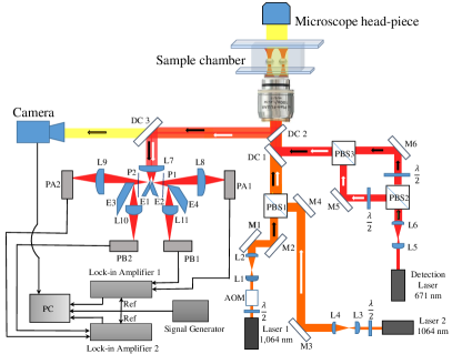
Figure A.1: A detailed schematic of the setup is shown. Key:$\frac{\lambda}{2}$: half-wave plate, L: lens, M: mirror, AOM: accousto optical modulator, PBS: polarising beam splitter, DC: dicroic mirror respectively, E: edge mirror, P: polariser, PA, PB: photodiodes.

Fig.A.2 (a) and (b) shows the histogram of position coordinate data that we acquire for the Brownian motion of driving particle B1 and driven particle B2, respectively. As is clear, the data are normally distributed in both traps and fit very well to Gaussians (shown in bold lines). To calibrate the traps and determine the trap stiffnesses, we measure the power spectral density (PSD) of the Brownian motion of each particle in the absence of the other. The results are shown in Fig.A.3(a) and (b). Each PSD is obtained by data blocking 100 points in the manner described in Ref. Berg-Sørensen and Flyvbjerg (2004). The Lorentzian fits to the data are good, and we obtain corner frequencies $\mathit{f_{c1}}=$461 Hz and $\mathit{f_{c2}}=$32.2 Hz for particles B1 and B2, which yield stiffnesses of $\mathit{k_{1}=}$69.2 $\mu N/m$ and $\mathit{k_{2}}$= 4.8 $\mu N/m$, respectively. For the two particle correlation experiments, as a consistency check, we determine the position cross-correlation function in time domain for B1 and B2 as shown in Fig.A.4. The data fits well to Eq.5 in Ref. Meiners and Quake (1999), with the constant parameters appropriately calculated for our case. Finally, we demonstrate the amplitude and phase response of the driving particle B1 as a function of the driving frequency in Fig.A.5(a) and (b), respectively. As expected, the amplitude decays with increasing frequency, while the phase is in sync with the drive at low frequencies and gradually lags behind as the frequency is increased.

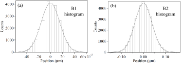
Figure A.2: Position histograms of (a) B1 (driving particle) and (b) B2 (driven particle). The solid black lines are corresponding Gaussian fits which show that the potentials are harmonic in nature.

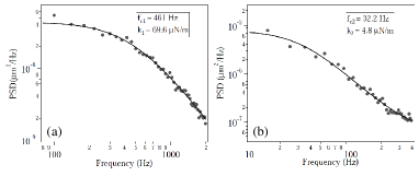
Figure A.3: Calibration of traps for B1 and B2. Experimentally measured data points are shown in filled gray circles, whereas the Lorentzian fit is denoted by the solid black line. (a) PSD for B1 which has a corner frequency $\mathit{f_{c1}=\mathrm{461}}$Hz and stiffness $\mathit{k_{1}=\mathrm{69.6}\>\mu}$N/m. (b) PSD for B2 which has a corner frequency $\mathit{f_{c1}=\mathrm{32.2}}$Hz and stiffness $\mathit{k_{1}=\mathrm{4.8}\>\mu}$N/m.

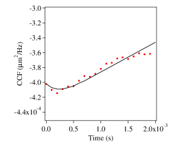
Figure A.4: Position cross-correlation in time domain. The filled red squares are experimentally measured points, while the solid line is the theoretically calculated cross-correlation.

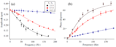
Figure A.5: Amplitude (a) and phase (b) response of driving particle B1 as a function of drive frequency.

Appendix B Theory

We outline below key steps in deriving the response and correlations functions on the Smoluchowski time scale, i.e. the over-damped limit, starting from Langevin equations

$$m_{i}\dot{\boldsymbol{v}_{i}} +\boldsymbol{\gamma}_{ij}\cdot\boldsymbol{v}_{j}+{\bf\boldsymbol{\nabla}}_{i}U=\boldsymbol{{\bf\xi}}_{i}$$ (6)

presented and explained in the main text.

(i) adiabatic elimination of momentum: in the first step, the momenta $m_{i}\boldsymbol{v}_{i}$ are adiabatically eliminated from the Langevin equations to obtain a contracted description in terms of the positions alone Gardiner (1984, 1985). This equation is valid on time scales $t\gg m_{i}/\gamma_{i}$. The heuristic of setting $m_{i}\boldsymbol{v}_{i}$ to zero in the Langevin equations yields the same result as the more systematic adiabatic elimination procedure, provided the multiplicative noise is interpreted correctly and the so-called “spurious” drift is included in the equation for the position increment van Kampen (1981, 1992). With these caveats, the resulting over-damped Langevin equations are

$$\boldsymbol{\gamma}_{ij}\cdot\boldsymbol{\dot{r}}_{j}+{\bf\boldsymbol{\nabla}}_{i}U=\boldsymbol{{\bf\xi}}_{i}.$$ (7)

(ii) linearization: in the next step, the equations are linearized in the small displacements $\boldsymbol{r}_{i}(t)=\boldsymbol{r}_{i}^{0}+\boldsymbol{u}_{i}(t)$, where $\boldsymbol{r}_{i}^{0}+\boldsymbol{u}_{i}^{0}(t)$ is the instantaneous position of the trap center. The mean distance between the trap centers, $\boldsymbol{\rho}=\boldsymbol{r}_{1}^{0}-\boldsymbol{r}_{2}^{0}$, is independent of time. This yields a linear equation of motion for the small displacements $\boldsymbol{u}_{i}$, where the friction tensors are now evaluated at the mean separation between the traps. The linearized Langevin equations are

$$\boldsymbol{\gamma}_{ij}(\boldsymbol{r}_{1}^{0},\boldsymbol{r}_{2}^{0})\cdot\dot{\boldsymbol{u}}_{j}+k_{i}\boldsymbol{u}_{i}-k_{i}\boldsymbol{u}_{i}^{0}(t)=\boldsymbol{\xi}_{i}$$ (8)

Note that these are 6 coupled stochastic ordinary differential equations.

(iii) decoupling through the use of symmetries: in this step, the symmetry of the friction tensors under translation, assuming all boundaries are remote, is used to express them as

$$\boldsymbol{\gamma}_{ij}=\gamma_{ij}^{\parallel}(\rho)\hat{\mathbf{\boldsymbol{\rho}}}\hat{\mathbf{\boldsymbol{\rho}}}+\gamma_{ij}^{\perp}(\rho)(\boldsymbol{I}-\hat{\mathbf{\boldsymbol{\rho}}}\hat{\mathbf{\boldsymbol{\rho}}}),$$ (9)

where $\gamma_{ij}^{||}(\rho)$ is the friction coefficient for relative motion along $\boldsymbol{\rho}$, the line joining the trap centers, while $\gamma_{ij}^{\perp}(\rho)$ is the corresponding quantity for motion perpendicular to $\boldsymbol{\rho}$. This motivates the decomposition of the displacement into components parallel and perpendicular to $\boldsymbol{\rho},$

$$\boldsymbol{u}_{i}=u_{i}^{\parallel}\hat{\mathbf{\boldsymbol{\rho}}}+\boldsymbol{u}_{i}^{\perp}\cdot(\boldsymbol{I}-\hat{\mathbf{\boldsymbol{\rho}}}\hat{\mathbf{\boldsymbol{\rho}}}).$$ (10)

Defining the force due to the driving of the trap as $\boldsymbol{f}_{i}(t)=k_{i}\boldsymbol{u}_{i}^{0}(t)$, averaging the equations over the noise, and using the two previous equations, we obtain 3 decoupled pairs of equations for each component of motion. For motion along the trap, the pair of coupled equations is

$$\gamma_{ij}^{||}\dot{u}_{j}^{||}+k_{i}u_{i}^{||}=f_{i}^{||}(t),$$ (11)

where the dependence of the friction coefficients on relative separation has been suppressed. The decoupling can be done before the linearization to give the same result; the two operations commute.

(iv) response function: in the final step the coupled equations are written as

$$\dot{u}_{i}^{||}+A_{ij}u_{j}^{||}=\mu_{ik}^{||}f_{k},$$ (12)

where $A_{ij}=\mu_{ij}^{||}k_{j}$ is a “response” matrix and the mobility matrix $\mu_{ij}^{||}$ is the inverse of the friction matrix, $\gamma_{ik}^{||}\mu_{kj}^{||}$=$\delta_{ij}$. The response function in the frequency domain, then, is Chaikin and Lubensky (2000)

$$\chi_{ij}^{||}(\omega)=(-i\omega\delta_{ik}+A_{ik})^{-1}\mu_{kj}^{||}.$$ (13)

Computing the inverse gives the following expression for the imaginary part of the response:

$$\text{Im}\left[\chi_{ij}^{||}(\omega)\right]= \frac{\omega}{(\text{det}A-\omega^{2})^{2}+(\omega\begin{tabular}[]{c}tr\end{tabular}A)^{2}}\left(\begin{array}[]{cc}\begin{tabular}[]{c}$\tfrac{k_{2}}{k_{1}}\mu_{22}^{\parallel}$\end{tabular}\text{det}A+\mu_{11}^{\parallel}\omega^{2}&-\mu_{12}^{\parallel}(\text{det}A-\omega^{2})\\ &\\ -\mu_{21}^{\parallel}(\text{det}A-\omega^{2})&\begin{tabular}[]{c}$\tfrac{k_{1}}{k_{2}}\mu_{11}^{\parallel}$\end{tabular}\text{det}A+\mu_{22}\omega^{2}\end{array}\right).$$ (20)

The modulus of the response of the first bead to the driving of the second bead is

$$|\chi_{21}^{||}| =\Big{|} \frac{i\omega\mu_{21}^{\parallel}}{\text{det}A-\omega^{2}-i\omega\begin{tabular}[]{c}tr\end{tabular}A}\Big{|},$$ (22)

which in non-zero only if there is viscous coupling, $\mu_{12}^{\parallel}\neq 0$. The modulus has a maximum at

$$\omega_{res}=\sqrt{\text{det}A}=\sqrt{\mu_{11}^{\parallel}\mu_{22}^{\parallel}k_{1}k_{2}\left(1-\frac{\mu_{12}^{\parallel}\mu_{21}^{\parallel}}{\mu_{11}^{\parallel}\mu_{22}^{\parallel}}\right)}.$$ (23)

(v) correlation function: To calculate the correlation function we set the modulation, $\boldsymbol{u}_{i}^{0}(t)$, of the traps to zero in Eq.(8) and project, as before, to obtain the Langevin equation for parallel displacement fluctuations

$$\boldsymbol{\gamma}_{ij}^{\parallel}\dot{u}_{j}^{\parallel}(t)+k_{i}u_{i}^{\parallel}(t)=\xi_{i}^{\parallel}(t),$$ (24)

$$\langle\xi_{i}^{\parallel}(t)\xi_{j}^{\parallel}(t^{\prime})\rangle=2k_{B}T\gamma_{ij}^{\parallel}\delta(t-t^{\prime}).$$ (25)

The Fourier amplitudes of the displacements are

$$u_{i}^{\parallel}(\omega) =(-i\omega\delta_{il}+A_{il})^{-1}\mu_{lk}^{||}\xi_{k}^{\parallel}(\omega),$$ (26)

and the correlation function is then

$$C_{ij}(\omega)=\langle u_{i}^{\parallel}(\omega)u_{j}^{{}^{\dagger}\parallel}(\omega)\rangle=$$

$$(-i\omega\delta_{il}+A_{il})^{-1}\mu_{lk}^{||}\langle\xi_{k}\xi_{k^{\prime}}\rangle\mu_{k^{\prime}m}^{||}(+i\omega\delta_{mj}+A_{mj}^{T})^{-1}.$$ (27)

Inserting the variance of the noise, the correlation function is

$$C_{ij}(\omega)= \frac{2k_{B}T}{(\text{det}A-\omega^{2})^{2}+(\omega\begin{tabular}[]{c}tr\end{tabular}A)^{2}}\left(\begin{array}[]{cc}\mu_{22}^{\parallel}k_{2}-i\omega&-\mu_{12}^{\parallel}k_{2}\\ \\ -\mu_{21}^{\parallel}k_{1}&\mu_{11}^{\parallel}k_{1}-i\omega\end{array}\right)\left(\begin{array}[]{cc}\mu_{11}^{\parallel}&\mu_{12}^{\parallel}\\ \\ \mu_{21}^{\parallel}&\mu_{22}^{\parallel}\end{array}\right)\left(\begin{array}[]{cc}\mu_{22}^{\parallel}k_{2}+i\omega&-\mu_{21}^{\parallel}k_{1}\\ \\ -\mu_{12}^{\parallel}k_{2}&\mu_{11}^{\parallel}k_{1}+i\omega\end{array}\right).$$ (38)

Completing the matrix multiplications, the final result is

$$C_{ij}(\omega)= \frac{2k_{B}T}{\omega}\text{Im}\left[\chi_{ij}^{||}(\omega)\right].$$ (39)

This provides an explicit verification of the fluctuation-dissipation relation for a pair of viscously coupled oscillators Kubo (1966).

References

- Nyquist (1928) H. Nyquist, Thermal agitation of electric charge in conductors, Phys. Rev. 32, 110 (1928).
- Callen and Welton (1951) H. B. Callen and T. A. Welton, Irreversibility and generalized noise, Phys. Rev. 83, 34 (1951).
- Kubo (1966) R. Kubo, The fluctuation-dissipation theorem, Rep. Prog. Phys. 29, 255 (1966).
- Seifert (2012) U. Seifert, Stochastic thermodynamics, fluctuation theorems and molecular machines, Rep. Prog. Phys. 75, 126001 (2012).
- Berthier and Biroli (2011) L. Berthier and G. Biroli, Theoretical perspective on the glass transition and amorphous materials, Rev. Mod. Phys. 83, 587 (2011).
- Fodor et al. (2016) É. Fodor, C. Nardini, M. E. Cates, J. Tailleur, P. Visco, and F. van Wijland, How far from equilibrium is active matter? Phys. Rev. Lett. 117, 038103 (2016).
- Mason and Weitz (1995) T. G. Mason and D. A. Weitz, Optical measurements of frequency-dependent linear viscoelastic moduli of complex fluids, Phys. Rev. Lett. 74, 1250–1253 (1995).
- Levine and Lubensky (2000) Alex J. Levine and T. C. Lubensky, One- and two-particle microrheology, Phys. Rev. Lett. 85, 1774–1777 (2000).
- Johnson (1928) J. B. Johnson, Thermal agitation of electricity in conductors, Phys. Rev. 32, 97 (1928).
- Derjaguin and Landau (1941) B. V. Derjaguin and L. D. Landau, Theory of the stability of strongly charged lyophobic sols and the adhesion of strongly charged particles in solutions of electrolytes, Acta Physicochim. USSR 14, 633–662 (1941).
- Verwey and Overbeek (1948) E. J. W. Verwey and J. Th. G. Overbeek, Theory of the stability of lyophobic colloids (Elsevier, Amsterdam, 1948).
- Stilgoe et al. (2011) A. B. Stilgoe, N. R. Heckenberg, T. A. Nieminen, and H. Rubinsztein-Dunlop, Phase-transition-like properties of double-beam optical tweezers, Phys. Rev. Lett. 107, 248101 (2011).
- Berg-Sørensen and Flyvbjerg (2004) K. Berg-Sørensen and H. Flyvbjerg, Power spectrum analysis for optical tweezers, Rev. Sci. Inst. 75, 594–612 (2004).
- Meiners and Quake (1999) J.-C. Meiners and S. R. Quake, Direct measurement of hydrodynamic cross correlations between two particles in an external potential, Phys. Rev. Lett. 82, 2211 (1999).
- Gardiner (1985) C. W. Gardiner, Handbook of stochastic methods, Vol. 3 (Springer Berlin, 1985).
- Ladd (1988) A. J. C. Ladd, Hydrodynamic interactions in a suspension of spherical particles, J. Chem. Phys. 88, 5051–5063 (1988).
- Mazur and Saarloos (1982) P. Mazur and W. van Saarloos, Many-sphere hydrodynamic interactions and mobilities in a suspension, Physica A: Stat. Mech. Appl. 115, 21–57 (1982).
- Cichocki et al. (1994) B. Cichocki, B. U. Felderhof, K. Hinsen, E. Wajnryb, and J. Blawzdziewicz, Friction and mobility of many spheres in Stokes flow, J. Chem. Phys. 100, 3780–3790 (1994).
- Singh and Adhikari (2016a) R. Singh and R. Adhikari, Universal hydrodynamic mechanisms for crystallization in active colloidal suspensions, Phys. Rev. Lett. 117, 228002 (2016a).
- Singh and Adhikari (2016b) R. Singh and R. Adhikari, Generalized Stokes laws for active colloids and their applications, arXiv:1603.05735 (2016b).
- Pozrikidis (1992) C. Pozrikidis, Boundary Integral and Singularity Methods for Linearized Viscous Flow (Cambridge University Press, 1992).
- Kim and Karrila (1992) S. Kim and S. J. Karrila, Microhydrodynamics: Principles and Selected Applications (Butterworth-Heinemann, 1992).
- Gardiner (1984) C. W. Gardiner, Adiabatic elimination in stochastic systems. i. formulation of methods and application to few-variable systems, Phys. Rev. A 29, 2814–2822 (1984).
- van Kampen (1981) N. G. van Kampen, Itô versus Stratonovich, J. Stat. Phys. 24, 175–187 (1981).
- van Kampen (1992) N. G. van Kampen, Stochastic processes in physics and chemistry, Vol. 1 (Elsevier, 1992).
- Klimontovich (1990) Y. L. Klimontovich, Itô, Stratonovich and kinetic forms of stochastic equations, Physica A: Stat. Mech. Appl. 163, 515–532 (1990).
- Klimontovich (1994) Y. L. Klimontovich, Nonlinear Brownian motion, Physics-Uspekhi 37, 737–766 (1994).
- Chaikin and Lubensky (2000) P. M. Chaikin and T. C. Lubensky, Principles of condensed matter physics, Vol. 1 (Cambridge Univ Press, 2000).