multicitedelim compcitedelim postnotedelim 297mm210mm* [] [] *32pc1.618 **1*** 2.5 *2* 2ex10mm0pt [nearest]   3.25ex plus 1ex -.2ex-1em-1em0pt manaartplain manaart0.5 manaartPorta ManaGeometry of maximum-entropy proofs manaart0 plain0 plain manainitialplain manainitial0.5 manainitialPorta ManaGeometry of maximum-entropy proofs manaart0 mydate mydate figure   *  

Geometry of maximum-entropy proofs:
stationary points, convexity,
Legendre transforms, exponential families

Most proofs of the traditional maximum-entropy formulae [jaynes1963, sivia1996_r2006, ch. 5]

$$\begin{gathered}\bm{p}=\frac{\exp(\bm{l}\bm{\varEpsilon}+\ln\bm{q})}{Z(\bm{l})}\qquad Z(\bm{l})=\bm{\varSigma}\exp(\bm{l}\bm{\varEpsilon}+\ln\bm{q})\qquad\frac{\partialup\ln Z}{\partialup\bm{l}}=\bm{\epsilon},\end{gathered}$$

with or without $\bm{q}$ terms, rely on the method of Lagrange multipliers, and many of them also show that the constrained maximization of the Shannon entropy is equivalent to the minimization of a “potential function” via a Lagrange transform. Examples are Mead & Papanicolaou’s *[§ II]meadetal1984 and Jaynes’s *[§ 11.6]jaynes1994_r2003 proofs.

This note is a geometric commentary on such proofs. Its purpose is to help you visualize some of the geometric structures involved and to explain more in detail why we end up minimizing a potential function to maximize the entropy, and how Lagrange transforms emerge. A synopsis of the main functions involved in the proof and of their very different properties is given at the end, together with a brief discussion of exponential families of probabilities, which appear in the proof.

I assume that you have some familiarity with the maximum-entropy method and the standard proof of its formulae, as in the references above. The geometric commentary is formulated in terms of the relative Shannon entropy [jaynes1963, § 4.c]kullback1982_r2006,good1983b, also called negative discrimination information [kullback1959_r1978, ch. 3], with respect to a reference distribution, because only this formulation is coordinate-independent in the continuum limit [hobsonetal1973, good1983b].

1 Notation

I hope you will indulge me in using vector-covector notation, which produces compact multidimensional formulae. A covector maps a vector into a scalar; it can be represented as a row matrix, and a vector as a column matrix. Here Latin letters will represent vectors; Greek, covectors. Juxtaposition of a vector and a covector always means their contraction or row-column multiplication, irrespective of their order; e.g. $\bm{\epsilon}\bm{l}=\bm{l}\bm{\epsilon}=\sumop\slimits@_{n}{}^{n}l_{n}$. I also use the convention that the logarithm maps vectors into covectors elementwise, and vice versa for the exponential; for example $\ln\bm{p}\coloneqq(\ln p_{1},\ln p_{2},\dotsc)$ and is a covector. Finally, convex means $\cup$-shaped, and concave means $\cap$-shaped.

2 Geometry of the proof

We have $K$ states $k\in\{1,\dotsc,K\}$ and $N$ observables $n\in\{1,\dotsc,N\}$. A measurement of the $n$th observable when the state is $k$ gives the value ^nk. These values are grouped into the operator $\bm{\varEpsilon}=({}^{nk})$ which maps vectors to covectors. The distribution of probabilities $\bm{p}=(p_{k})$, a vector, expresses our uncertainty about the actual state. The expectations for the $N$ observables under our state of uncertainty are $\bm{\varEpsilon}\bm{p}$. The $K$-dimensional covector $\bm{\varSigma}=(1,\dotsc,1)$ and allows us very suggestively to write $\bm{\varSigma}\bm{p}=\sumop\slimits@_{k}p_{k}$.

We want to choose a probability distribution for which the expectations are constrained to values $\bm{\epsilon}=({}_{n})$, represented by a covector. But the constraints $\bm{\varEpsilon}\bm{p}=\bm{\epsilon}$ don’t select a unique $\bm{p}$ if $N<K-1$. We therefore ask that that the distribution meet an additional requirement that makes it unique: $\bm{p}$ must maximize the relative Shannon entropy $H(\bm{p})\coloneqq-\bm{p}\ln\bm{p}+\bm{p}\ln\bm{q}$, under those constraints, with respect to a reference distribution $\bm{q}$. We denote this unique distribution $\bm{p}_{\bm{\epsilon}}$, and the corresponding maximum value of the entropy $S(\bm{\epsilon})\coloneqq H(\bm{p}_{\bm{\epsilon}})$; it’s called the Gibbs entropy. The Shannon and Gibbs entropies are different functions, of completely different quantities.

To find the constrained maximum of the relative Shannon entropy we use the method of Lagrange multipliers [boydetal2004_r2009, ch. 5]. I warmly recommend Rockafellar’s *rockafellar1993 brilliant review of the various meanings of Lagrange multipliers, which offers plenty of geometric insights.

With scalar $u$ and vector $\bm{l}=(l_{n})$, define the function of $(\bm{p},u,\bm{l})$ with parameter

$$L_{\bm{\epsilon}}(\bm{p},u,\bm{l})\coloneqq-\bm{p}\ln\bm{p}+\bm{p}\ln\bm{q}+u\,(\bm{\varSigma}\bm{p}-1)+\bm{l}\,(\bm{\varEpsilon}\bm{p}-\bm{\epsilon}),$$ (1)

usually called Lagrangian [fangetal1997, boydetal2004_r2009]. It’s defined on the $(K+N+1)$-dimensional manifold ${\bm{\mathrm{R}}_{\geqslant 0}}^{K}\times\bm{\mathrm{R}}^{N+1}$, our “base manifold”. Proofs of the maximum-entropy formulae with linear constraints show that the Lagrangian $L_{\bm{\epsilon}}(\bm{p},u,\bm{l})$ has a unique saddle point $(\bm{p}_{\bm{\epsilon}},u_{\bm{\epsilon}},\bm{l}_{\bm{\epsilon}})$, and the saddle-point coordinate $\bm{p}_{\bm{\epsilon}}$ is the maximum-entropy solution.

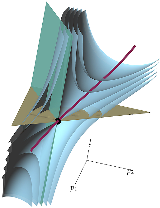
$K=3$, $N=1$. Equations $\bm{\varSigma}\bm{p}-1=0$ (3b) and $u=1-\ln Z(\bm{l})$ (4b) are identically satisfied. Black dot: saddle point $(\bm{p}_{\bm{\epsilon}},u_{\bm{\epsilon}},\bm{l}_{\bm{\epsilon}})$.
Blue surfaces: contours of $L_{\bm{\epsilon}}(\bm{p},u,\bm{l})$ (1).
Thick purplish-red curve: submanifold $-\ln\bm{p}+\ln\bm{q}+\bm{l}\bm{\varEpsilon}+u\bm{\varSigma}=0$ (3a) or $\bm{p}=\exp(\bm{l}\bm{\varEpsilon}+\ln\bm{q})/Z(\bm{l})$ (4a); its intersection with the blue surfaces are the “contours” (points) of $G_{\bm{\epsilon}}(\bm{l})$, eq. (5).
Vertical bluish-green plane: submanifold $\bm{\varEpsilon}\bm{p}-\bm{\epsilon}=0$ (3c).
Horizontal greenish-yellow plane: submanifold $\bm{\varEpsilon}\exp(\bm{l}\bm{\varEpsilon}+\ln\bm{q})/Z(\bm{l})=\bm{\epsilon}$ (4c), which is the plane $\bm{l}=\bm{l}_{\bm{\epsilon}}$.

?figurename? 1: (Colour-blind-friendly palette by Tol [*]tol2009_r2012)

Figure 1 depicts our constrained maximization problem in the simplest nontrivial case: $K=3$, $N=1$. Our base manifold has therefore $5$ dimensions. The $3$-dimensional space represented in the figure is a section of our base manifold, obtained by selecting specific values of the coordinates $p_{3}$ and $u$ as functions – (3a) and (4b)–(4d) below – of the remaining ones.

The blue surfaces in fig. 1 are the contour levels of the Lagrangian (1). Their saddle is clearly visible. The saddle point is the black dot. Note that a section roughly parallel to the $\bm{l}$ axis is made within the figure for clearer visibility of the surfaces and curves involved.

The value of the Lagrangian $L_{\bm{\epsilon}}$ at the saddle point is the value of the Gibbs entropy:

$$L_{\bm{\epsilon}}(\bm{p}_{\bm{\epsilon}},u_{\bm{\epsilon}},\bm{l}_{\bm{\epsilon}})\equiv S(\bm{\epsilon}).$$ (2)

It’s easy to check this: the constraint terms in (1) vanish at the saddle-point and what remains is the maximized Shannon entropy, that is, the Gibbs entropy.

Our saddle-point problem reduces, thanks to the continuous differentiability of the Lagrangian, to the system of three vector equations

$$-\ln\bm{p}+\ln\bm{q}+\bm{l}\bm{\varEpsilon}+u\bm{\varSigma} =0,$$ (3a)

$$\bm{\varSigma}\bm{p}-1 =0,$$ (3b)

$$\bm{\varEpsilon}\bm{p}-\bm{\epsilon} =0.$$ (3c)

They are the implicit equations of three submanifolds in our $(K+N+1)$-dimensional base manifold. The first is curved, $(N+1)$-dimensional. The second is flat, $(K+N)$-dimensional, and contains the simplex of normalized probability distributions; the $3$-dimensional space depicted in fig. 1 is the intersection of our $5$-dimensional base manifold with this submanifold, and therefore eq. (3b) is identically satisfied in the figure. The third submanifold is flat, $(K+1)$-dimensional; it is the vertical bluish-green plane in the figure. The saddle point is the intersection of these three submanifolds.

The vector equations above can be recombined and written as a system of three new vector equations:

$$\bm{p}=\frac{1}{Z(\bm{l})}\exp(\bm{l}\bm{\varEpsilon}+\ln\bm{q}),$$ (4a)

$$u=1-\ln Z(\bm{l}),$$ (4b)

$$\frac{1}{Z(\bm{l})}\bm{\varEpsilon}\exp(\bm{l}\bm{\varEpsilon}+\ln\bm{q})=\bm{\epsilon},$$ (4c)

$$\text{with }Z(\bm{l})\coloneqq\bm{\varSigma}\exp(\bm{l}\bm{\varEpsilon}+\ln\bm{q}).$$ (4d)

The first is the parametric equation of a curved $(N+1)$-dimensional submanifold, which is also submanifold of (3b). The second is the parametric equation of a curved $(K+N)$-dimensional submanifold; the $3$-dimensional space of fig. 1 is the intersection of this submanifold, besides (3b), with our $5$-dimensional base manifold; eq. (4b) is thus also identically satisfied in the figure. The third equation in the system above is the implicit equation of a flat $(K+1)$ dimensional submanifold. This equation determines a unique value $\bm{l}_{\bm{\epsilon}}$, so it is simply the equation of the $(K+1)$-plane $\bm{l}=\bm{l}_{\bm{\epsilon}}$, the horizontal greenish-yellow plane in fig. 1. These three submanifolds (4), are distinct from the previous three (3), but they also intersect at the saddle point. The function $\ln Z(\bm{l})$ defined in (4d) is called normalization function or partition function.

Note that we could have formulated our constrained-maximization problem by imposing the normalization (3b) from the very beginning, for example defining $p_{K}=1-p_{1}-p_{2}-\dotsb$. The multiplier $u$ and eqs (3b), (4b) wouldn’t have appeared, and our base manifold would have been $(K+N-1)$-dimensional. Figure 1 can also be interpreted this way.

The system (3a) & (3b) is equivalent to the system (4a) & (4b), as can be verified by substitution; that is, the $N$-dimensional intersection submanifold of the first pair is also the intersection of the second pair. This submanifold is the thick purplish-red curve in the figure. Projected onto the simplex of probability distributions – that is, disregarding the $u$ and $\bm{l}$ dimensions – this submanifold is an subset of the latter called an exponential family. Exponential families are briefly discussed in § 4. The saddle point is the intersection of this $N$-dimensional submanifold with either the $(K+1)$-plane (3c) or the $(K+1)$-plane (4c).

The saddle point $(\bm{p}_{\bm{\epsilon}},u_{\bm{\epsilon}},\bm{l}_{\bm{\epsilon}})$ could therefore be found by finding the root $\bm{l}=\bm{l}_{\bm{\epsilon}}$ of eq. (4c), and substituting this root in $\bigl{(}\bm{p}(\bm{l}),u(\bm{l})\bigr{)}$, the parametric form of eqs (4a) & (4b). But it turns out that we do not need to solve eq. (4c). There’s an interesting development.

Looking at fig. 1 we notice that the $N$-dimensional manifold $\bigl{(}\bm{p}(\bm{l}),u(\bm{l})\bigr{)}$ extends from the pommel to the cantle of the saddle (if the lower part is the cantle the horse is rearing). This was a priori not necessary: by construction this submanifold must pass through the saddle point, but it could have done so by going from the pommel down to the flaps of the saddle. It couldn’t have made a U-turn back to the pommel, however, because that implies the presence of a wedge, whereas our manifold is continuously differentiable.

This placement of the $N$-dimensional submanifold implies that if we ride it we see the values of the Lagrangian decrease until we reach the saddle point, and then increase again. The saddle point is therefore the minimum of the Lagrangian restricted to the $N$-dimensional submanifold. This is true for the $N=1$ case of our figure, but it generalizes to larger $N$; here’s how.

Consider the restriction of the Lagrangian $L_{\bm{\epsilon}}$, eq. (1), to the $N$-dimensional submanifold. This restriction, denoted , is usually called the potential function. It’s by construction a function of $\bm{l}$ alone, from eqs (4a) and (4b):

$${}_{\bm{\epsilon}}(\bm{l})\coloneqq L_{\bm{\epsilon}}[\bm{p}(\bm{l}),u(\bm{l}),\bm{l}]\equiv\ln Z(\bm{l})-\bm{l}\bm{\epsilon}.$$ (5)

In fig. 1 the intersections of the blue surfaces with the thick purplish-red curve are the “contours” – just points in this case – of this function. The Hessian matrix of its second derivatives has non-negative eigenvalues: a simple calculation and a look at (4) reveal that this is in fact the covariance matrix of the observable :

$$\frac{{}^{2}{}_{\bm{\epsilon}}}{\partialup l_{n}\partialup l_{m}}\equiv\frac{{}^{2}\ln Z}{\partialup l_{n}\partialup l_{m}}=\sumop\slimits@_{k}{}^{nk}{}^{mk}p_{k}(\bm{l})-\sumop\slimits@_{k}{}^{nk}p_{k}(\bm{l})\,\sumop\slimits@_{k}{}^{mk}p_{k}(\bm{l}),$$ (6)

and covariance matrices have non-negative eigenvalues [feller1966_r1971, § III.5]. The potential function is therefore convex – strictly so, without flat regions, owing to the differential properties of the logarithm. Calculation of its unique minimum by derivation leads to eq. (4c). The conclusion is that the potential function is convex in $\bm{l}$, and the saddle point of $L_{\bm{\epsilon}}$ in the $(K+N+1)$-dimensional base manifold is the unique minimum of in the $N$-submanifold.

This is the geometric reason why the constrained-maximization problem in $K$ dimensions for the Shannon entropy $H(\bm{p})$ can be transformed into an unconstrained-minimization problem in $N$ dimensions for the potential function $\ln Z(\bm{l})-\bm{l}\bm{\epsilon}$. The latter is usually called the dual problem [fangetal1997, boydetal2004_r2009]. This fact is enormously useful for numerical computations: it allows us to use convex optimization techniques [pressetal1988_r2007] to find the extremizing Lagrange multipliers $\bm{l}_{\bm{\epsilon}}$ and thence the distribution $\bm{p}_{\bm{\epsilon}}$ and the Gibbs entropy $S(\bm{\epsilon})\coloneqq H(\bm{p}_{\bm{\epsilon}})$. See Rockafellar’s *rockafellar1993 insightful discussion in this respect too.

But the geometry of this extremization problem has further surprises.

The Gibbs entropy $S(\bm{\epsilon})$ is, from its definition, equal to $L_{\bm{\epsilon}}(\bm{p}_{\bm{\epsilon}},u_{\bm{\epsilon}},\bm{l}_{\bm{\epsilon}})\equiv{}_{\bm{\epsilon}}(\bm{l}_{\bm{\epsilon}})\equiv\ln Z(\bm{l}_{\bm{\epsilon}})-\bm{l}_{\bm{\epsilon}}\bm{\epsilon}$, which is the unique minimum of ${}_{\bm{\epsilon}}(\bm{l})$. We can write this as

$$S(\bm{\epsilon})=\inf_{\smash{\bm{l}}}[\ln Z(\bm{l})-\bm{l}\bm{\epsilon}].$$ (7)

This formula is the proper definition of the negative Legendre transform of the normalization function $\ln Z(\bm{l})$, that is, its negative convex conjugate [fenchel1949]. This means that the Gibbs entropy $S(\bm{\epsilon})$ is a concave function of . The concavity of the Gibbs entropy is an important property, completely distinct from the concavity of the Shannon entropy $H(\bm{p})$. I said “proper” Legendre transform because the physics literature often defines the latter without the extremization indicated by “$\inf$” or “$\sup$”. Such simplified definition breaks down if the transformed function is not strictly convex – which may happen in important physical situations. See Wightman’s illuminating and pedagogical discussion [wightman1979, pp. xxiv–xxix].

From the involutive property of the Legendre transform see refs above, the normalization function $\ln Z(\bm{l})$ is the negative Legendre transform of the negative Gibbs entropy:

$$\ln Z(\bm{l})=\inf_{\smash{\bm{\epsilon}}}[-S(\bm{\epsilon})-\bm{\epsilon}\bm{l}].$$ (8)

The appearance of these Lagrange transforms has many important connections with statistical mechanics; for interesting recent developments see Chomaz & al.’s *chomazetal2006,chomazetal2005b reviews. I refrain from speaking about the relationship between the maximum-entropy method: it’s subtle and already too often oversimplified in the literature.

3 Synopsis of the main functions

It’s important to keep the main functions involved in the proof well-distinct from one another:

• The Shannon entropy $H(\bm{p})$ is a function of the probability distribution $\bm{p}$. It’s concave in $\bm{p}$. It isn’t the Legendre transform of anything.

• The Gibbs entropy

  $$S(\bm{\epsilon})\equiv\sup_{\smash{\bm{p}}}^{\smash{\bm{\varEpsilon}\bm{p}=\bm{\epsilon}}}H(\bm{p})\equiv\inf_{\smash{\bm{l}}}[\ln\bm{\varSigma}\exp(\bm{l}\bm{\varEpsilon}+\ln\bm{q})-\bm{l}\bm{\epsilon}]\equiv\inf_{\smash{\bm{l}}}[\ln Z(\bm{l})-\bm{l}\bm{\epsilon}]$$

  is a function of the expectation values . It’s concave in . It’s the constrained maximum of the relative Shannon entropy, the unconstrained minimum of the potential function, and the negative Legendre transform of the normalization function.

• The normalization function, partition function, or free entropy

  $$\ln Z(\bm{l})\equiv\ln\bm{\varSigma}\exp(\bm{l}\bm{\varEpsilon}+\ln\bm{q})\equiv\inf_{\smash{\bm{\epsilon}}}[-S(\bm{\epsilon})-\bm{\epsilon}\bm{l}]$$

  is a function of the Lagrange multipliers $\bm{l}$. It’s convex in $\bm{l}$. It’s the negative Legendre transform of the negative Gibbs entropy.

• The potential function ${}_{\bm{\epsilon}}(\bm{l})\equiv\ln Z(\bm{l})-\bm{l}\bm{\epsilon}$ is a function of the Lagrange multipliers $\bm{l}$ with a parametric dependence on the expectation values . It’s convex in $\bm{l}$. It isn’t the Legendre transform of anything. Not to be confused with the Gibbs entropy.

4 Exponential families

The maximum-entropy method is essentially a function that maps a set of observables, a set of observable constraints, and a reference distribution to a probability distribution: $(\bm{\varEpsilon},\bm{\epsilon},\bm{q})\mapsto\bm{p}$. From this point of view all other quantities appearing in its proof and formulae are just auxiliary quantities – including the Lagrange multipliers $\bm{l}$.

But the parametric submanifold of probabilities $\bm{p}(\bm{l})$, eq. (4a):

$$\bm{p}(\bm{l})=\frac{1}{Z(\bm{l})}\exp(\bm{l}\bm{\varEpsilon}+\ln\bm{q}),\qquad Z(\bm{l})\coloneqq\bm{\varSigma}\exp(\bm{l}\bm{\varEpsilon}+\ln\bm{q}),$$ (9)

has a meaning and an importance of its own, outside of the maximum-entropy method. It is an example of exponential family. Exponential families are particular submanifolds of a simplex of probability distributions characterized by an exponential parametric form like the above or more general see below for references.

The figures on the right show an example of $2$-dimensional exponential family for the case with four states, $K=4$, two observables, $N=2$, having values

$$({}^{nk})\equiv\begin{pmatrix}{}^{1\,k}\\ {}^{2\,k}\end{pmatrix}=\begin{pmatrix}0&1&2&3\\ 1&1&0&0\end{pmatrix},$$ (10)

and a uniform reference distribution $\bm{q}$. The black lines are the edges of the simplex of probability distributions $\bm{p}$, a tetrahedron. The exponential-family submanifold is the yellow surface, the same in both figures.

In the top figure the reddish-purple curves are equally-spaced $(l_{1},l_{2})$ coordinates for the parametrization in terms of the Lagrange multipliers, $\bm{l}\coloneqq(l_{1},l_{2})\in\bm{\mathrm{R}}^{2}$. In the bottom figure the green curves are equally-spaced $({}_{1},{}_{2})$ coordinates for the parametrization in terms of the expectations, $\bm{\epsilon}\coloneqq({}_{1},{}_{2})\in[0,3]\times[0,1]$.

The relation between these two coordinate systems, eq. (3c), is highly non-linear. The $\bm{l}$ coordinates have the advantage of parametrizing $\bm{p}(\bm{l})$ in closed form, eq. (4a), but are uncongenial to the convex structure of the simplex of probability distributions; their non-compact range must in fact cover a compact set. The coordinates are clearly more congenial to the convex structure of the probability simplex, but they do not lend themselves to a parametrization $\bm{p}(\bm{\epsilon})$ in closed form. Both $\bm{l}$- and -parametrizations are therefore important.

The Bernoulli, Poisson, exponential, normal distributions belong to exponential families. See Bernardo & Smith *[ch. 4, esp. § 4.5.3]bernardoetal1994_r2000 for a thorough discussion of these families, Barndorff-Nielsen *barndorffnielsen1978_r2014 for their relation with Lagrange transforms, Dawid *dawid2013 for a broader context. Exponential families appear in the probability calculus when we assume that a particular fixed set of quantities from some measurements is all we need to make inferences about other similar measurements, a condition called sufficiency [ch. 4, esp. § 4.5.3]bernardoetal1994_r2000barndorffnielsen1978_r2014,dawid2013,andersen1970. The fact that they appear in the maximum-entropy formulae thus suggests a relation between maximum-entropy and sufficiency. A recent work which I don’t fully understand [portamana2017] argues, however, that this relation has some downsides, and maximum-entropy distributions are best related to so-called exchangeable models [bernardoetal1994_r2000, § 4.3].

prenote(“van $X$” is listed under V; similarly for other prefixes, regardless of national conventions.)