$f_{1}(1285)\to e^{+}e^{-}$ decay and direct $f_{1}$ production in $e^{+}e^{-}$ collisions

Abstract

The width of the $f_{1}(1285)\to e^{+}e^{-}$ decay is calculated in the vector meson dominance model. The result depends on the relative phase between two coupling constants describing $f_{1}\to\rho^{0}\gamma$ decay. The width $\Gamma(f_{1}\to e^{+}e^{-})$ is estimated to be $\simeq 0.07\textendash 0.19$ eV. Direct $f_{1}$ production in $e^{+}e^{-}$ collisions is discussed, and the $e^{+}e^{-}\to f_{1}\to a_{0}\pi\to\eta\pi\pi$ cross section is calculated. Charge asymmetry in the $e^{+}e^{-}\to\eta\pi^{+}\pi^{-}$ reaction due to interference between $e^{+}e^{-}\to f_{1}$ and $e^{+}e^{-}\to\eta\rho^{0}$ amplitudes is studied.

I Introduction

High-luminosity electron-positron colliders are powerful tools for measuring electronic widths of hadronic resonances with positive charge parity, $C=+1$. The idea of such measurements was put forward many years ago Altarelli:67 ; Vainshtein:71 . Several experiments in search of direct production of $C$-even resonances in $e^{+}e^{-}$ collisions were performed, and very low upper limits on the leptonic widths of $\eta^{\prime}$, $f_{2}(1270)$, $a_{2}(1320)$, and $X(3872)$ mesons were set snd1 ; kmd-3 ; snd2 ; besIII .

The explanation of the smallness of the leptonic widths of $C$-even resonances is that corresponding decays proceed via two virtual photons and therefore are suppressed by a factor of $\alpha^{4}$, where $\alpha$ is the fine structure constant.

In this paper we consider $1^{++}$ meson $f_{1}(1285)$, its decay into the $e^{+}e^{-}$ pair, and its direct production in $e^{+}e^{-}$ collisions. The process $e^{+}e^{-}\to f_{1}\to mesons$ is still not measured and may be studied at the VEPP-2000 $e^{+}e^{-}$ collider in experiments with the SND and CMD-3 detectors.

There is a quite extensive list of literature on the production of $1^{++}$ resonances in $e^{+}e^{-}$ annihilation. The direct production of $1^{++}$ states through the neutral current was evaluated many years ago in the nonrelativistic quarkonium model Kaplan:78 . The calculation of the width $\Gamma(\chi_{1}\to e^{+}e^{-})$ was performed in the quarkonium and vector meson dominance models (VMD) Kuhn:79 . There are also some recent papers devoted to $X(3872)$ and $\chi_{c1}$ decays into the $e^{+}e^{-}$ pair and their production in $e^{+}e^{-}$ collisions (see Denig:14 ; Czyz:16 ; Czyz:17 ; Kivel:16 and references therein). The production of $1^{++}$ resonances $R$ in two-photon collisions ($e^{+}e^{-}\to e^{+}e^{-}R$) was also extensively studied both theoretically Kopp:74 ; Renard:84 ; Cahn:87 ; Schuler:98 and experimentally Gidal:87 ; Aihara:88 ; Achard:02 .

The paper is organized as follows. In Sec. II a simple estimate of the width $\Gamma(f_{1}\to e^{+}e^{-})$ is given. In Sec. III we discuss the amplitude of the $f_{1}\to\gamma^{*}\gamma^{*}$ transition in a model-independent way. In Sec. IV amplitudes and coupling constants describing the $f_{1}\to\rho^{0}\gamma$ decay are studied and constrained using experimental data. Section V describes a choice of $f_{1}\to\gamma^{*}\gamma^{*}$ form factors and the calculation of $\Gamma(f_{1}\to e^{+}e^{-})$. In Sec. VI we estimate the $e^{+}e^{-}\to f_{1}\to\eta\pi\pi$ cross section. In Sec. VII charge asymmetry in the $e^{+}e^{-}\to\eta\pi^{+}\pi^{-}$ process is studied. And finally, in Sec. VIII we conclude.

II Simple estimate of $f_{1}\to e^{+}e^{-}$ decay width

It is convenient to start our discussion with the simple analysis of the $f_{1}\to e^{+}e^{-}$ decay (see the tree diagram in Fig. 1).

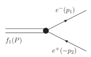
Figure 1: The Feynman tree diagram for the $f_{1}\to e^{+}e^{-}$ decay.

The electron and positron produced in this decay are ultrarelativistic in the $f_{1}$ rest frame. So, in this frame $e^{+}$ and $e^{-}$ can be considered as massless and having the definite helicities. An additional argument for neglecting the electron mass can be given. In Ref. Yang:12 the width of the $\chi_{c1}\to l^{+}l^{-}$ decay was calculated with the finite lepton mass, and it was found that the mass effects are negligible.

To construct the decay amplitude, we notice that the decay $e^{+}$ and $e^{-}$ may in principle be produced in two polarization states, with the same ($j_{z}=0$) or opposite ($j_{z}=\pm 1$) helicities. Here $j_{z}$ is the projection of the total $e^{+}e^{-}$ angular momentum $j$ onto the $z$ axis, which is directed along the $e^{-}$ momentum in the $f_{1}$ rest frame. Because of conservation laws (in particular, conservation of $P$ and $C$ parities) only one polarization state with opposite helicities of $e^{+}$ and $e^{-}$ is realized. Therefore, there is only one $P$- and $C$-even invariant amplitude for the $f_{1}\to e^{+}e^{-}$ decay, which is written as

$$M(f_{1}\to e^{+}e^{-})=F_{A}\alpha^{2}\widetilde{e}_{\mu}\bar{u}\gamma^{\mu}\gamma^{5}v,$$ (1)

where $\widetilde{e}_{\mu}$ is the $C$-even axial vector describing the $f_{1}$ meson, $\bar{u}\gamma^{\mu}\gamma^{5}v=j_{A}^{\mu}$ is the axial current, and $F_{A}$ is the dimensionless coupling constant. Since $f_{1}$ meson is $C$-even, it decays into $e^{+}e^{-}$ via two virtual photons as depicted in Fig. 2. This explains the origin of the factor $\alpha^{2}$ in (1).

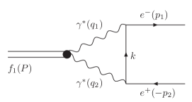
Figure 2: One-loop diagram of the $f_{1}\to e^{+}e^{-}$ decay with two intermediate photons.

Using the amplitude (1) it is easy to calculate the decay width

$$\Gamma(f_{1}\to e^{+}e^{-})=\frac{\alpha^{4}|F_{A}|^{2}}{12\pi}m_{f},$$ (2)

where $m_{f}$ is the $f_{1}$ mass, $m_{f}=1282.0$ MeV pdg16 .

For a naive estimate, it is natural to assume that the coupling constant $F_{A}$ is of the order of unity, $|F_{A}|\sim 1$. In (1) we have already written explicitly the small factor $\alpha^{2}$, and there are not any additional small factors. So, we obtain that $\Gamma(f_{1}\to e^{+}e^{-})\sim 0.1$ eV.

In what follows we calculate this width in a certain model and find that this simple estimate is correct by the order of magnitude.

III Model-independent description of $f_{1}\to e^{+}e^{-}$ amplitude

To calculate the width $\Gamma(f_{1}\to e^{+}e^{-})$ more accurately, we should know the amplitude of the $f_{1}\to\gamma^{*}\gamma^{*}$ transition (see Fig. 2). This amplitude must be symmetric with respect to the permutation of virtual photons and must vanish when both photons are on shell ($f_{1}\to\gamma\gamma$ decay is forbidden by the Landau-Yang theorem Landau:48 ). Also the amplitude of the $f_{1}\to\gamma^{*}\gamma^{*}$ transition must contain two independent terms, corresponding to two different polarization states in the $f_{1}$ rest frame. These states can be denoted as $TT$ (when both virtual photons are transversal) and $TL$ (when the first photon is transversal and the second photon is longitudinal). States $TL$ and $LT$ are the same here due to the photon identity. The polarization state $LL$ (when both virtual photons are longitudinal) does not exist, because the $f_{1}$ meson is axial one.

So, the $f_{1}\to\gamma^{*}\gamma^{*}$ amplitude is parametrized in general by two dimensionless form factors, $F_{1}(q_{1}^{2},q_{2}^{2})$ and $F_{2}(q_{1}^{2},q_{2}^{2})$, which are functions of photon momenta squared. We choose this amplitude in the following form based on amplitudes used, e.g., in Refs. Kuhn:79 ; Kopp:74 ; Renard:84 :

$$M(f_{1}\to\gamma^{*}\gamma^{*})=\frac{\alpha}{m^{2}_{f}}F_{1}(q_{1}^{2},q_{2}^{2})i\epsilon_{\mu\nu\rho\sigma}q_{1}^{\mu}e_{1}^{*\nu}q_{2}^{\rho}e_{2}^{*\sigma}\widetilde{e}^{\tau}(q_{1}-q_{2})_{\tau}+\\ +\frac{\alpha}{m^{2}_{f}}\left\{F_{2}(q_{1}^{2},q_{2}^{2})i\epsilon_{\mu\nu\rho\sigma}q_{1}^{\mu}e_{1}^{*\nu}\widetilde{e}^{\rho}\left[q_{2}^{\sigma}e_{2}^{*\lambda}q_{2\lambda}-e_{2}^{*\sigma}q_{2}^{2}\right]+F_{2}(q_{2}^{2},q_{1}^{2})i\epsilon_{\mu\nu\rho\sigma}q_{2}^{\mu}e_{2}^{*\nu}\widetilde{e}^{\rho}\left[q_{1}^{\sigma}e_{1}^{*\lambda}q_{1\lambda}-e_{1}^{*\sigma}q_{1}^{2}\right]\right\},$$ (3)

where $e_{1}$, $e_{2}$, and $\widetilde{e}$ are the polarization vectors of the first photon, second photon, and $f_{1}$ meson, respectively. In this expression the form factor $F_{1}$ corresponds to transversal photons ($TT$), and the form factor $F_{2}$ describes a combination of $TT$ and $LT$ polarization states.

Because of the Bose symmetry form factor $F_{1}(q_{1}^{2},q_{2}^{2})$ must be antisymmetric, $F_{1}(q_{1}^{2},q_{2}^{2})=-F_{1}(q_{2}^{2},q_{1}^{2})$. As it should be, the amplitude (3) vanishes when both photons are on shell. Indeed, the first term vanishes because of $F_{1}(0,0)=0$, while all terms in the last line of (3) vanish because $q^{2}=0$ and $e^{\lambda}q_{\lambda}=0$ for real photons.

We substitute this $f_{1}\to\gamma^{*}\gamma^{*}$ amplitude into the expression for the one-loop diagram (see Fig. 2) and perform straightforward calculation in the Feynman gauge, using the identity

$$i\epsilon_{\mu\nu\rho\sigma}\gamma^{\sigma}=\left(\gamma_{\mu}\gamma_{\nu}\gamma_{\rho}-g_{\mu\nu}\gamma_{\rho}+g_{\mu\rho}\gamma_{\nu}-g_{\nu\rho}\gamma_{\mu}\right)\gamma^{5},$$ (4)

and Dirac equations for massless electron and positron, $\bar{u}\hat{p}_{1}=0$ and $\hat{p}_{2}v=0$. This leads to the following expression for the $f_{1}\to e^{+}e^{-}$ amplitude:

$$M(f_{1}\to e^{+}e^{-})=-\frac{16\pi i\alpha^{2}}{m^{2}_{f}}\widetilde{e}^{\mu}P^{\nu}\bar{u}\gamma^{\lambda}\gamma^{5}v\int\frac{d^{4}k}{(2\pi)^{4}}\frac{k_{\mu}k_{\nu}k_{\lambda}}{k^{2}q_{1}^{2}q_{2}^{2}}F_{1}(q_{1}^{2},q_{2}^{2})-\\ -\frac{8\pi i\alpha^{2}}{m^{2}_{f}}\widetilde{e}^{\mu}\bar{u}\gamma^{\nu}\gamma^{5}v\int\frac{d^{4}k}{(2\pi)^{4}}\frac{k_{\mu}k_{\nu}}{k^{2}q_{1}^{2}q_{2}^{2}}\left\{F_{2}(q_{1}^{2},q_{2}^{2})q_{2}^{2}+F_{2}(q_{2}^{2},q_{1}^{2})q_{1}^{2}\right\}+\\ +\frac{4\pi i\alpha^{2}}{m^{2}_{f}}\widetilde{e}_{\mu}\bar{u}\gamma^{\mu}\gamma^{5}v\int\frac{d^{4}k}{(2\pi)^{4}}\frac{1}{k^{2}q_{1}^{2}q_{2}^{2}}\left\{F_{2}(q_{1}^{2},q_{2}^{2})\left[k^{2}(p_{1}p_{2}+p_{1}k-p_{2}k)-2q_{2}^{2}(p_{1}k)+2q_{2}^{2}k^{2}\right]+\right.\\ \left.+F_{2}(q_{2}^{2},q_{1}^{2})\left[k^{2}(p_{1}p_{2}+p_{1}k-p_{2}k)+2q_{1}^{2}(p_{2}k)+2q_{1}^{2}k^{2}\right]\right\},$$ (5)

where $q_{1}=p_{1}-k$ and $q_{2}=p_{2}+k$.

IV Constants of $f_{1}\to\rho^{0}\gamma$ decay from experimental data

One cannot calculate the width $\Gamma(f_{1}\to e^{+}e^{-})$ in a model-independent way, because the explicit form of functions $F_{1}$ and $F_{2}$ in (5) is unknown. So, we have to choose some reasonable model.

We assume that the main contribution to the amplitude $M(f_{1}\to e^{+}e^{-})$ comes from the diagram depicted in Fig. 3, where both virtual photons are coupled with the $f_{1}$ meson via intermediate $\rho^{0}$ mesons. However, we do not take into account here direct $f_{1}\gamma^{*}\gamma^{*}$, $f_{1}\rho^{0}\gamma^{*}$, and $f_{1}\phi\gamma^{*}$ couplings. One of the arguments is that dimensional analysis shows that form factors $F_{1}$ and $F_{2}$ should decrease rapidly with increasing momentum $k$ in order to avoid divergences in (3.3). Even if form factors $F_{1}$ and $F_{2}$ behave as $1/k^{2}$ (it corresponds to $f_{1}\rho^{0}\gamma^{*}$ or $f_{1}\phi\gamma^{*}$ couplings), then the amplitude (3.3) diverges logarithmically. This is the hint that both virtual photons couple with the $f_{1}$ meson via some massive vector mesons. In such a case form factors $F_{1}$ and $F_{2}$ behave as $1/k^{4}$ and the amplitude (3.3) does not diverge. Experimental data show that one of the main $f_{1}$ decay channels, $f_{1}\to 4\pi$ [$\mathcal{B}(f_{1}\to 4\pi)\approx 33\%$], proceeds mainly via the intermediate $\rho\rho$ state Barberis:00 . Other evidence of this mechanism is a large (5.5%) branching ratio of radiative $f_{1}\to\rho^{0}\gamma$ decay pdg16 . So, the assumption that $f_{1}\rho^{0}\rho^{0}$ coupling gives the main contribution to the amplitude $M(f_{1}\to e^{+}e^{-})$ looks quite reasonable.

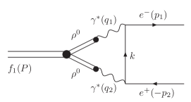
Figure 3: The VMD mechanism of the $f_{1}\to e^{+}e^{-}$ decay with two intermediate $\rho^{0}$ mesons.

The amplitude $f_{1}\to\rho^{0*}\rho^{0*}$ can be written by analogy with (3),

$$M(f_{1}\to\rho^{0*}\rho^{0*})=\frac{1}{m^{2}_{f}}h_{1}(q_{1}^{2},q_{2}^{2})i\epsilon_{\mu\nu\rho\sigma}q_{1}^{\mu}e_{1}^{*\nu}q_{2}^{\rho}e_{2}^{*\sigma}\widetilde{e}^{\tau}(q_{1}-q_{2})_{\tau}+\\ +\frac{1}{m^{2}_{f}}\left\{h_{2}(q_{1}^{2},q_{2}^{2})i\epsilon_{\mu\nu\rho\sigma}q_{1}^{\mu}e_{1}^{*\nu}\widetilde{e}^{\rho}\left[q_{2}^{\sigma}e_{2}^{*\lambda}q_{2\lambda}-e_{2}^{*\sigma}q_{2}^{2}\right]+h_{2}(q_{2}^{2},q_{1}^{2})i\epsilon_{\mu\nu\rho\sigma}q_{2}^{\mu}e_{2}^{*\nu}\widetilde{e}^{\rho}\left[q_{1}^{\sigma}e_{1}^{*\lambda}q_{1\lambda}-e_{1}^{*\sigma}q_{1}^{2}\right]\right\}.$$ (6)

Some parameters of the model can be constrained from experimental data on $f_{1}\to\rho^{0}\gamma$ decay. The corresponding amplitude can be obtained from (3), where all particles should be considered on shell. For $q_{1}^{2}=m_{\rho}^{2}$ (here $m_{\rho}=775.26$ MeV pdg16 is the $\rho^{0}$ mass), $q_{2}^{2}=0$, and $e_{1}q_{1}=e_{2}q_{2}=0$ we obtain

$$M(f_{1}\to\rho^{0}\gamma)=\frac{\alpha}{m^{2}_{f}}g_{1}i\epsilon_{\mu\nu\rho\sigma}p^{\mu}\epsilon^{*\nu}q^{\rho}e^{*\sigma}\widetilde{e}^{\tau}(p-q)_{\tau}-\frac{\alpha m^{2}_{\rho}}{m^{2}_{f}}g_{2}i\epsilon_{\mu\nu\rho\sigma}\widetilde{e}^{\mu}\epsilon^{*\nu}q^{\rho}e^{*\sigma},$$ (7)

where $e,\epsilon$, and $\widetilde{e}$ are polarization vectors of photon, $\rho^{0}$, and $f_{1}$, respectively; $p$ and $q$ are momenta of $\rho^{0}$ and photon. This amplitude contains two complex coupling constants, $g_{1}$ and $g_{2}$, because there are two different polarization states. The first state is when $\rho^{0}$ meson polarization is longitudinal ($L$) in the $f_{1}$ rest frame, and the second one is when $\rho^{0}$ meson polarization is transversal ($T$). In the expression (7) the coupling constant $g_{1}$ corresponds to the $T$ polarization state of $\rho^{0}$, and $g_{2}$ corresponds to a combination of $L$ and $T$ polarization states. In the $f_{1}$ rest frame the ratio of the longitudinal and transversal parts of this amplitude is the following:

$$\frac{M_{L}(f_{1}\to\rho^{0}\gamma)}{M_{T}(f_{1}\to\rho^{0}\gamma)}=\frac{\sqrt{\xi}g_{2}}{(1-\xi)g_{1}+\xi g_{2}},$$ (8)

where $\xi=m^{2}_{\rho}/m^{2}_{f}\approx 0.37$.

Now it is straightforward to calculate the width of $f_{1}\to\rho^{0}\gamma$ decay,

$$\Gamma(f_{1}\to\rho^{0}\gamma)=\frac{\alpha^{2}}{96\pi}m_{f}(1-\xi)^{3}\left[(1-\xi)^{2}|g_{1}|^{2}+\xi(1+\xi)|g_{2}|^{2}+2\xi(1-\xi)|g_{1}||g_{2}|\cos{\delta}\right].$$ (9)

Since the parameters $g_{1}$ and $g_{2}$ do not correspond to different polarization states [see the comment after Eq. (3)], the interference term does not vanish after summation over polarizations, and expression (9) contains $\delta=\phi_{1}-\phi_{2}$, which is the relative phase of the complex constants $g_{1}$ and $g_{2}$.

The expression (9) represents one relation between three unknown parameters $g_{1}$, $g_{2}$, and $\delta$. One more relation can be derived from the polarization experiments. The ratio of the contributions of two $\rho^{0}$ helicity states, $r=\rho_{LL}/\rho_{TT}=3.9\pm 0.9\pm 1.0$, was determined in the VES experiment Amelin:95 from the analysis of angular distributions in the reaction $f_{1}\to\rho^{0}\gamma\to\pi^{+}\pi^{-}\gamma$,

$$|M(f_{1}\to\rho^{0}\gamma\to\pi^{+}\pi^{-}\gamma)|^{2}\sim\rho_{LL}\cos^{2}{\theta}+\rho_{TT}\sin^{2}{\theta},$$ (10)

where $\rho_{LL}$ and $\rho_{TT}$ are density matrix elements corresponding to longitudinal and transverse $\rho^{0}$ mesons, respectively; $\theta$ is the angle between $\pi^{+}$ and $\gamma$ momenta in the $\rho^{0}$ rest frame. Integrating over $d(\cos{\theta})$, one easily finds that

$$\Gamma(f_{1}\to\rho^{0}\gamma\to\pi^{+}\pi^{-}\gamma)\sim\rho_{LL}+2\rho_{TT}.$$ (11)

Calculation of $|M(f_{1}\to\rho^{0}\gamma\to\pi^{+}\pi^{-}\gamma)|^{2}$ with the amplitude (7) leads to the following ratio of the coefficients at $\cos^{2}{\theta}$ and $\sin^{2}{\theta}$:

$$r=\frac{2\xi|g_{2}|^{2}}{(1-\xi)^{2}|g_{1}|^{2}+\xi^{2}|g_{2}|^{2}+2\xi(1-\xi)|g_{1}||g_{2}|\cos{\delta}},$$ (12)

which equals to $\rho_{LL}/\rho_{TT}$ from Ref. Amelin:95 .

The decay width (9) can be presented as a sum of contributions of different polarization states,

$$\Gamma(f_{1}\to\rho^{0}\gamma)=\frac{\alpha^{2}}{96\pi}m_{f}(1-\xi)^{3}\left[g_{TT}+g_{LL}\right],$$ (13)

where

$$g_{TT}=(1-\xi)^{2}|g_{1}|^{2}+\xi^{2}|g_{2}|^{2}+2\xi(1-\xi)|g_{1}||g_{2}|\cos{\delta},$$ (14)

$$g_{LL}=\xi|g_{2}|^{2}.$$ (15)

Note that $g_{LL}/g_{TT}=r/2=\rho_{LL}/2\rho_{TT}$ in agreement with (11).

Recently CLAS Collaboration at Jefferson Laboratory (JLab) published the results of the first measurements of the $f_{1}$ meson in the photoproduction reaction $\gamma p\to f_{1}p$ off a proton target Dickson:16 . The first estimate of the cross section of this reaction in the JLab kinematics and suggestion that its measurement with the CLAS detector is possible were reported in Ref. Kochelev:09 .

According to the data of CLAS Collaboration, the branching ratio $\mathcal{B}(f_{1}\to\rho^{0}\gamma)$ equals $(2.5\pm 0.9)\%$, which is substantially smaller than the PDG value, $(5.5\pm 1.3)\%$. A few theoretical models consistent with this result are proposed already Wang:17 ; Wang:2017 ; Osipov:17 . The total $f_{1}$ width measured by CLAS Collaboration $\Gamma_{f}^{CLAS}=(18.4\pm 1.4)$ MeV is also considerably smaller than the PDG value, $\Gamma_{f}=(24.1\pm 1.0)$ MeV. Therefore, below we present the results of our calculations for PDG averages and CLAS Collaboration values as well.

Using the experimental result $r=3.9\pm 0.9\pm 1.0$ Amelin:95 we obtain

$$\alpha^{2}g_{TT}=\frac{96\pi\mathcal{B}(f_{1}\to\rho^{0}\gamma)\Gamma_{f}}{m_{f}(1-m^{2}_{\rho}/m^{2}_{f})^{3}}\frac{2}{r+2}=0.41\pm 0.14,\hskip 28.45274pt\alpha^{2}g_{TT}^{CLAS}=0.14\pm 0.06,$$ (16)

$$\alpha^{2}g_{LL}=\frac{96\pi\mathcal{B}(f_{1}\to\rho^{0}\gamma)\Gamma_{f}}{m_{f}(1-m^{2}_{\rho}/m^{2}_{f})^{3}}\frac{r}{r+2}=0.81\pm 0.22,\hskip 28.45274pt\alpha^{2}g_{LL}^{CLAS}=0.28\pm 0.18,$$ (17)

and find the magnitude of coupling constant $g_{2}$,

$$\alpha|g_{2}|=1.5\pm 0.2,\hskip 28.45274pt\alpha|g_{2}|^{CLAS}=0.87\pm 0.18.$$ (18)

It is seen that values of this coupling constant obtained for PDG and CLAS data are essentially different.

It is impossible to extract the magnitude of the constant $g_{1}$ and/or the phase $\delta$ from the experimental data. From Eq. (14) we obtain the following relation between the absolute value of $g_{1}$ and two other parameters:

$$|g_{1}|=\frac{1}{1-\xi}\left(-\xi|g_{2}|\cos{\delta}+\sqrt{(\xi|g_{2}|\cos{\delta})^{2}+g_{TT}-\xi g_{LL}}\right).$$ (19)

Taking into account that $-1\leq\cos{\delta}\leq 1$, we obtain

$$0.16\lesssim\alpha|g_{1}|\lesssim 1.9,\hskip 28.45274pt0.09\lesssim\alpha|g_{1}|^{CLAS}\lesssim 1.1,$$ (20)

for the central values of $g_{TT}$, $g_{LL}$, and $|g_{2}|$; see (16), (17), and (18). The upper and lower limits on $|g_{1}|$ correspond to $\delta=\pi$ and $\delta=0$, respectively.

It is seen that there is a large uncertainty in the value of $|g_{1}|$. Indeed, $|g_{1}|$ could be of the same order of magnitude as $|g_{2}|$, if $\delta$ is close to $\pi$, and of the order of magnitude smaller, if $\delta$ is close to 0. Moreover, quite large experimental uncertainties in the polarization experiment Amelin:95 allow one to speculate that $|g_{1}|$ could be very small or even negligible. Indeed, in the case $g_{1}=0$ one obtains from (12) that $r=2/\xi\approx 5.5$, which is not very far from the central value $r=3.9$.

There are some papers concerning $f_{1}\to\rho^{0}\gamma$ decay, where the amplitude $M(f_{1}\to\rho^{0}\gamma)$ is parametrized only by one constant Kochelev:09 ; Wang:2017 ; Osipov:17 . Therein the ratio of $M_{L}(f_{1}\to\rho^{0}\gamma)$ to $M_{T}(f_{1}\to\rho^{0}\gamma)$ is equal to $m_{f}/m_{\rho}=1/\sqrt{\xi}$, which coincides with the expression (8) at $g_{1}=0$. So, these models correspond to our model at $g_{1}=0$.

There are also papers where the amplitude $M(f_{1}\to\rho^{0}\gamma)$ is parametrized by two constants; see, e.g., Ref. Lutz:08 . Therein two relations between parameters of $f_{1}\to\rho^{0}\gamma$ decay are obtained using $\Gamma(f_{1}\to\rho^{0}\gamma)$ and $r=\rho_{LL}/\rho_{TT}$. In this paper the $f_{1}$ meson is considered as the molecular state and $f_{1}\to\rho^{0}\gamma$ decay is studied in the chiral effective field theory.

V Calculation of $f_{1}\to e^{+}e^{-}$ decay width

In order to construct the amplitude $M(f_{1}\to e^{+}e^{-})$ (see Fig. 3) we consider also the transition $\rho^{0*}\to\gamma^{*}$. The Lagrangian of such a transition in gauge-invariant form reads

$$\mathcal{L}=\frac{1}{2}g_{\rho\gamma}V^{\mu\nu}F_{\mu\nu},$$ (21)

where $g_{\rho\gamma}$ is the coupling constant, and $V_{\mu\nu}$ and $F_{\mu\nu}$ are the tensors of the $\rho^{0}$ meson field and electromagnetic field, respectively. Therefore, we obtain the corresponding amplitude,

$$M(\rho^{0}\to\gamma)=g_{\rho\gamma}(q^{2}g_{\mu\nu}-q_{\mu}q_{\nu})\epsilon^{\mu}e^{*\nu},$$ (22)

where $q$ is the momentum, and $\epsilon$ and $e$ are polarization vectors of the $\rho^{0}$ meson and photon, respectively. The coupling constant $g_{\rho\gamma}$ can be found from $\rho^{0}\to e^{+}e^{-}$ decay width,

$$\Gamma(\rho^{0}\to e^{+}e^{-})=\frac{1}{3}\alpha g_{\rho\gamma}^{2}m_{\rho}.$$ (23)

Using the experimental values $\Gamma(\rho^{0}\to e^{+}e^{-})\approx 6.98$ keV and $m_{\rho}=775.26$ MeV pdg16 we derive $g_{\rho\gamma}\approx 0.06$.

Now we can compare the amplitudes described by diagrams in Figs. 2 and 3 and obtain the relation between form factors $F_{1}$ and $h_{1}$, $F_{2}$ and $h_{2}$,

$$\alpha F_{1,2}(q_{1}^{2},q_{2}^{2})=\frac{g^{2}_{\rho\gamma}q_{1}^{2}q_{2}^{2}}{(q_{1}^{2}-m_{\rho}^{2}+im_{\rho}\Gamma_{\rho})(q_{2}^{2}-m_{\rho}^{2}+im_{\rho}\Gamma_{\rho})}h_{1,2}(q_{1}^{2},q_{2}^{2}),$$ (24)

where $\Gamma_{\rho}=147.8$ MeV is the $\rho^{0}$-meson width. In what follows we consider $\Gamma_{\rho}$ as a constant parameter, because to account for its dependence on the momentum squared, $\Gamma_{\rho}(q^{2})$, seems to be beyond the accuracy of our calculation.

Comparison (6) with (7) leads to relations

$$\lim_{q_{2}^{2}\to 0}q_{2}^{2}h_{1}(m_{\rho}^{2},q_{2}^{2})=-\frac{\alpha g_{1}}{g_{\rho\gamma}}\left(m_{\rho}^{2}-im_{\rho}\Gamma_{\rho}\right),$$ (25)

$$\lim_{q_{2}^{2}\to 0}q_{2}^{2}h_{2}(q_{2}^{2},m_{\rho}^{2})=-\frac{\alpha g_{2}}{g_{\rho\gamma}}\left(m_{\rho}^{2}-im_{\rho}\Gamma_{\rho}\right).$$ (26)

Now let us consider $f_{1}\to\pi^{+}\pi^{-}\pi^{+}\pi^{-}$ decay. Experimental data indicate that the main contribution to it is given by the intermediate state with two virtual $\rho$ mesons Barberis:00 (see Fig. 4). The vertex $f_{1}\rho\rho$ contains the form factors $h_{1}$ and $h_{2}$ of our model. Certainly, these form factors should meet the requirements that the result of the calculation of the $f_{1}\to\pi^{+}\pi^{-}\pi^{+}\pi^{-}$ decay width should be in a good agreement with the experimental value.

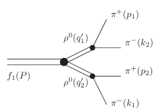
Figure 4: Feynman diagrams of $f_{1}\to\pi^{+}\pi^{-}\pi^{+}\pi^{-}$ decay.

We parametrize the $\rho^{0}\to\pi^{+}\pi^{-}$ amplitude as

$$M(\rho^{0}\to\pi^{+}\pi^{-})=if_{\rho\pi\pi}e_{\mu}p^{\mu},$$ (27)

where $e_{\mu}$ is the polarization vector of the $\rho^{0}$ meson, and $p^{\mu}$ is the momentum of the $\pi^{+}$ meson. We neglect the $q^{2}$ dependence of $f_{\rho\pi\pi}$ and obtain the following value:

$$f_{\rho\pi\pi}=\left(\frac{192\pi\Gamma(\rho^{0}\to\pi^{+}\pi^{-})}{m_{\rho}(1-4m_{\pi}^{2}/m_{\rho}^{2})^{3/2}}\right)^{1/2}\approx 11.9,$$ (28)

where $\Gamma(\rho^{0}\to\pi^{+}\pi^{-})\approx\Gamma_{\rho}=147.8$ MeV, and $m_{\pi}=139.57$ MeV is the mass of $\pi^{\pm}$ mesons.

Taking into account that form factor $F_{1}(q_{1}^{2},q_{2}^{2})$ is antisymmetric, and using relations (24), (25), and (26) as a hint, we write the form factors $F_{1}$ and $F_{2}$ as

$$F_{1}(q_{1}^{2},q_{2}^{2})=\frac{g_{\rho\gamma}g_{1}(m_{\rho}^{2}-im_{\rho}\Gamma_{\rho})(q_{2}^{2}-q_{1}^{2})}{(q_{1}^{2}-m_{\rho}^{2}+im_{\rho}\Gamma_{\rho})(q_{2}^{2}-m_{\rho}^{2}+im_{\rho}\Gamma_{\rho})},$$ (29)

$$F_{2}(q_{1}^{2},q_{2}^{2})=\frac{g_{\rho\gamma}g_{2}(m_{\rho}^{2}-im_{\rho}\Gamma_{\rho})(-m_{\rho}^{2})}{(q_{1}^{2}-m_{\rho}^{2}+im_{\rho}\Gamma_{\rho})(q_{2}^{2}-m_{\rho}^{2}+im_{\rho}\Gamma_{\rho})}.$$ (30)

The result of numerical calculation with corresponding form factors $h_{1}$ and $h_{2}$ is shown in Fig. 5. The solid line depicts the branching ratio of $f_{1}\to\pi^{+}\pi^{-}\pi^{+}\pi^{-}$ decay, $\mathcal{B}_{c}$, calculating for the central values: $r=\rho_{LL}/\rho_{TT}=3.9$ and $\mathcal{B}(f_{1}\to\rho^{0}\gamma)=5.5\%$ or $\mathcal{B}^{CLAS}(f_{1}\to\rho^{0}\gamma)=2.5\%$. Quite large experimental uncertainties $\Delta r\approx 1.3$ and $\Delta\mathcal{B}(f_{1}\to\rho^{0}\gamma)=1.3\%$ or $\Delta\mathcal{B}^{CLAS}(f_{1}\to\rho^{0}\gamma)=0.9\%$ may lead to the substantial deviation of $\mathcal{B}(f_{1}\to\pi^{+}\pi^{-}\pi^{+}\pi^{-})$ from its central values $\mathcal{B}_{c}$. The results, corresponding to one standard deviation of $\mathcal{B}$ from its central value, are shown in Fig. 5 by dashed and dotted lines. The shaded horizontal band in Fig. 5 indicates values allowed experimentally, $\mathcal{B}(f_{1}\to\pi^{+}\pi^{-}\pi^{+}\pi^{-})=\left(11.0^{+0.7}_{-0.6}\right)\%$.

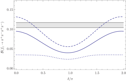
PDG data		CLAS Collaboration data

Figure 5: The branching ratio of the $f_{1}\to\pi^{+}\pi^{-}\pi^{+}\pi^{-}$ decay for the certain choice of the form factors $F_{1}(q_{1}^{2},q_{2}^{2})$ and $F_{2}(q_{1}^{2},q_{2}^{2})$; see Eqs. (29) and (30). The solid line corresponds to the $f_{1}\to\pi^{+}\pi^{-}\pi^{+}\pi^{-}$ branching ratio calculated using the central values: $r=3.9$ and $\mathcal{B}(f_{1}\to\rho^{0}\gamma)=5.5\%$ or $\mathcal{B}^{CLAS}(f_{1}\to\rho^{0}\gamma)=2.5\%$. Dashed and dotted lines indicate $1\sigma$ deviations for $\mathcal{B}(f_{1}\to\pi^{+}\pi^{-}\pi^{+}\pi^{-})$. The shaded horizontal band denotes the value allowed experimentally, $\mathcal{B}(f_{1}\to\pi^{+}\pi^{-}\pi^{+}\pi^{-})=\left(11.0^{+0.7}_{-0.6}\right)\%$.

It is seen from Fig. 5 that we still cannot derive the exact value of the phase $\delta$ in our model because of large uncertainties of the model parameters. Therefore, in what follows we treat $\delta$ as a free parameter.

To calculate the $f_{1}\to e^{+}e^{-}$ branching ratio, we substitute the expressions for $F_{1}(q_{1}^{2},q_{2}^{2})$ and $F_{2}(q_{1}^{2},q_{2}^{2})$ into (5) and perform the numerical calculations; then, comparing the answer with (1), we obtain the following result for the constant $F_{A}$:

$$F_{A}\simeq-\alpha g_{1}\left(0.22+0.25i\right)-\alpha g_{2}\left(0.75+0.57i\right).$$ (31)

It is convenient to express complex numbers $g_{1}$ and $g_{2}$ in polar form as $g_{1}=|g_{1}|\cdot e^{i\phi_{1}}$ and $g_{2}=|g_{2}|\cdot e^{i\phi_{2}}$, respectively. Then using $\delta=\phi_{1}-\phi_{2}$ one can write the absolute square of the constant $F_{A}$ as

$$|F_{A}|^{2}\simeq\Big{|}e^{i\delta}\cdot\alpha|g_{1}|\cdot\left(0.22+0.25i\right)+\alpha|g_{2}|\cdot\left(0.75+0.57i\right)\Big{|}^{2}.$$ (32)

Since $\alpha|g_{2}|\sim 1$ and $\alpha|g_{1}|\lesssim 1$ [see (18) and (20)], then $|F_{A}|\sim 1$, as expected. In particular, for central values of $|g_{1}|$ and $|g_{2}|$ we get $|F_{A}|\simeq 1.12$ for $\delta=0.7\pi$, $|F_{A}|\simeq 1.28$ for $\delta=1.3\pi$, and $|F_{A}|^{CLAS}\simeq 0.85$ for $\delta=0$.

Now it is straightforward to calculate the branching ratio $\mathcal{B}(f_{1}\to e^{+}e^{-})$ as a function of $\delta$. Corresponding plots are shown in Fig. 6, where the solid line denotes $\mathcal{B}(f_{1}\to e^{+}e^{-})$ calculating for the central values: $r=3.9$ and $\mathcal{B}(f_{1}\to\rho^{0}\gamma)=5.5\%$ or $\mathcal{B}^{CLAS}(f_{1}\to\rho^{0}\gamma)=2.5\%$. Dashed and dotted lines indicate $1\sigma$ deviations.

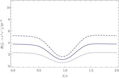
PDG data		CLAS Collaboration data

Figure 6: The branching ratio $\mathcal{B}(f_{1}\to e^{+}e^{-})$ as a function of the relative phase $\delta$ in our model. The solid line corresponds to $\mathcal{B}(f_{1}\to e^{+}e^{-})$ calculated for the central values: $r=3.9$ and $\mathcal{B}(f_{1}\to\rho^{0}\gamma)=5.5\%$ or $\mathcal{B}^{CLAS}(f_{1}\to\rho^{0}\gamma)=2.5\%$. The dashed and dotted lines indicate $1\sigma$ deviations from the $\mathcal{B}(f_{1}\to e^{+}e^{-})$ central value.

We see that these functions are almost constant for $-\pi/2<\delta<\pi/2$ and have a minimum near $\delta=\pi$. Such behavior can easily be understood from (32) and (19). Indeed, when $\cos{\delta}>0$, the value of $|g_{1}|$ is quite small due to cancellation in (19), so the main contribution to $|F_{A}|^{2}$ is given by $|g_{2}|$ and the corresponding factor, which are both independent of $\delta$. However, when $\delta$ is close to $\pi$ then $|g_{1}|$ is comparable with $|g_{2}|$, so a quite strong cancellation occurs in (32), and therefore $\mathcal{B}(f_{1}\to e^{+}e^{-})$ is minimal.

It is seen from Figs. 5 and 6 that in our model the branching ratio $\mathcal{B}(f_{1}\to e^{+}e^{-})$ should be taken in the range from $3\cdot 10^{-9}$ for $\delta\simeq\pi$ to $8\cdot 10^{-9}$ for $\delta=0$, and from $4\cdot 10^{-9}$ for $\delta^{CLAS}=0$ to $5\cdot 10^{-9}$ for $\delta^{CLAS}\simeq\pm 0.3\pi$,

$$\mathcal{B}(f_{1}\to e^{+}e^{-})\simeq(3\textendash 8)\cdot 10^{-9},\hskip 28.45274pt\mathcal{B}^{CLAS}(f_{1}\to e^{+}e^{-})\simeq(4\textendash 5)\cdot 10^{-9},$$ (33)

and the corresponding decay width is

$$\Gamma(f_{1}\to e^{+}e^{-})\simeq 0.07\textendash 0.19\ {\rm eV},\hskip 28.45274pt\Gamma^{CLAS}(f_{1}\to e^{+}e^{-})\simeq 0.07\textendash 0.10\ {\rm eV}.$$ (34)

The values of the branching ratio and the decay width obtained for CLAS data lie in a more narrow interval than the corresponding values obtained for PDG data. However, both ranges of $\Gamma(f_{1}\to e^{+}e^{-})$ values are in good agreement with the naive estimate $\Gamma\sim 0.1$ eV (see the end of Sec. II).

VI Estimate of $e^{+}e^{-}\to f_{1}\to\eta\pi\pi$ cross section

Let us estimate the cross section of the process $e^{+}e^{-}\to f_{1}\to\eta\pi\pi$, which can be used for the study ofdirect $f_{1}$ production in $e^{+}e^{-}$ collisions. Here, the $f_{1}\to\eta\pi\pi$ decay proceeds mainly (approximately with 70% probability pdg16 ) through the intermediate $a_{0}(980)$ meson; see Figs. 7 and 8.

Figure 7: The diagrams for $e^{+}e^{-}$ annihilation into the $\eta\pi^{+}\pi^{-}$ final state via the intermediate $f_{1}$ and $a_{0}$ mesons.

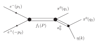
Figure 8: The diagram for $e^{+}e^{-}$ annihilation into the $\eta\pi^{0}\pi^{0}$ final state via the intermediate $f_{1}$ and $a_{0}$ mesons.

The branching ratio of the $f_{1}\to a_{0}\pi$ decay is $(36\pm 7)\%$ pdg16 . Using the isospin symmetry we obtain $\mathcal{B}(f_{1}\to a_{0}^{+}\pi^{-})=\mathcal{B}(f_{1}\to a_{0}^{-}\pi^{+})=\mathcal{B}(f_{1}\to a_{0}^{0}\pi^{0})=1/3\,\mathcal{B}(f_{1}\to a_{0}\pi)\approx 12\%$.

Since the $a_{0}$ meson is scalar and the $\pi$ meson is pseudoscalar, the amplitude of the $f_{1}\to a_{0}\pi$ decay can be written as

$$M(f_{1}\to a_{0}\pi)=ig\chi_{a}^{*}\widetilde{\phi}_{\pi}^{*}\widetilde{e}_{\mu}p_{\pi}^{\mu},$$ (35)

where $g$ is the dimensionless coupling constant; $\chi_{a}$, $\widetilde{\phi}_{\pi}$, and $\widetilde{e}_{\mu}$ are wave functions of $a_{0}$, $\pi$ and $f_{1}$ mesons, respectively; and $p_{\pi}$ is the momentum of the $\pi$ meson.

The cross section of the $e^{+}e^{-}\to f_{1}\to a_{0}\pi$ process can easily be calculated,

$$\sigma(e^{+}e^{-}\to f_{1}\to a_{0}\pi)=\frac{12\pi}{m_{f}^{2}}\mathcal{B}(f_{1}\to a_{0}\pi)\mathcal{B}(f_{1}\to e^{+}e^{-}),$$ (36)

where the center-of-mass energy equals the mass of the $f_{1}$ meson, $\sqrt{s}=m_{f}$. Using the experimental value for the branching ratio $\mathcal{B}(f_{1}\to a_{0}\pi)=0.36\pm 0.07$ and the result of our calculations (33) for $\mathcal{B}(f_{1}\to e^{+}e^{-})$, we obtain

$$\sigma(e^{+}e^{-}\to f_{1}\to a_{0}\pi)\simeq 7.8\textendash 30\ {\rm pb},\hskip 28.45274pt\sigma^{CLAS}(e^{+}e^{-}\to f_{1}\to a_{0}\pi)\simeq 10\textendash 20\ {\rm pb}.$$ (37)

Assuming that the $a_{0}$ meson decays only into the $\eta\pi$ final state and using the relation $\mathcal{B}(f_{1}\to a_{0}^{\pm}\pi^{\mp}\to\eta\pi^{+}\pi^{-})=2\,\mathcal{B}(f_{1}\to a_{0}^{0}\pi^{0}\to\eta\pi^{0}\pi^{0})=2/3\,\mathcal{B}(f_{1}\to a_{0}\pi\to\eta\pi\pi)$, we obtain the following estimates:

$$\sigma(e^{+}e^{-}\to f_{1}\to a_{0}^{\pm}\pi^{\mp}\to\eta\pi^{+}\pi^{-})\simeq 5.2\textendash 20\ {\rm pb},\hskip 8.53581pt\sigma^{CLAS}(e^{+}e^{-}\to f_{1}\to a_{0}^{\pm}\pi^{\mp}\to\eta\pi^{+}\pi^{-})\simeq 7\textendash 13.3\ {\rm pb},$$ (38)

$$\sigma(e^{+}e^{-}\to f_{1}\to a_{0}^{0}\pi^{0}\to\eta\pi^{0}\pi^{0})\simeq 2.6\textendash 10\ {\rm pb},\hskip 8.53581pt\sigma^{CLAS}(e^{+}e^{-}\to f_{1}\to a_{0}^{0}\pi^{0}\to\eta\pi^{0}\pi^{0})\simeq 3.5\textendash 6.7\ {\rm pb}.$$ (39)

It is seen that the values of cross sections obtained for PDG and CLAS data are in reasonable agreement within uncertainties. However, the values of $\sigma^{CLAS}$ lie in a narrower range. Therefore, one can hope that future precise experiments could make it possible to distinguish between $\sigma^{PDG}$ and $\sigma^{CLAS}$.

VII Charge asymmetry in $e^{+}e^{-}\to\eta\pi^{+}\pi^{-}$ process

Though the cross section of the $e^{+}e^{-}\to f_{1}\to\eta\pi^{0}\pi^{0}$ process is twice less than that of $e^{+}e^{-}\to f_{1}\to\eta\pi^{+}\pi^{-}$, the former is more convenient for the study of direct $f_{1}$ production in $e^{+}e^{-}$ collisions. Indeed, the $e^{+}e^{-}\to\eta\pi^{0}\pi^{0}$ reaction proceeds only through two-photon annihilation, since $C$ parity of the $\eta\pi^{0}\pi^{0}$ final state is positive. Therefore, there is no background from one-photon annihilation, and the $e^{+}e^{-}\to f_{1}\to\eta\pi^{0}\pi^{0}$ cross section can be measured directly. According to the estimate (39), the lower bound on this cross section is quite small, but it can be measured in a special experiment at the VEPP-2000 collider in Novosibirsk.

In contrast, the $e^{+}e^{-}\to\eta\pi^{+}\pi^{-}$ reaction proceeds mainly through one-photon annihilation, which is described quite well by the VMD model with intermediate $\rho^{\prime}(1450)$ and $\rho^{0}(770)$ mesons Aulchenko:15 , as depicted in Fig. 9.

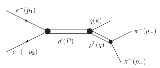
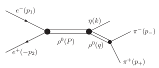
Figure 9: The diagrams for $e^{+}e^{-}$ annihilation into the $\eta\pi^{+}\pi^{-}$ final state via intermediate vector $\rho^{\prime}(1450)$ and $\rho^{0}(770)$ mesons.

The measured $e^{+}e^{-}\to\eta\pi^{+}\pi^{-}$ Born cross section is about 500 pb at $\sqrt{s}=m_{f}$ Aulchenko:15 . According to the estimate (38), the $e^{+}e^{-}\to f_{1}\to a_{0}^{\pm}\pi^{\mp}\to\eta\pi^{+}\pi^{-}$ cross section constitutes only several percent of the total $e^{+}e^{-}\to\eta\pi^{+}\pi^{-}$ cross section, and its measurement is a rather complicated task. One possibility to overcome this difficulty is to investigate the two-photon annihilation channel $e^{+}e^{-}\to f_{1}\to\eta\pi^{+}\pi^{-}$ through $C$-odd effects, which arise from the interference of $C$-odd one-photon and $C$-even two-photon amplitudes.

The annihilation $e^{+}e^{-}\to\rho\to\eta\pi^{+}\pi^{-}$ was studied theoretically in Ref. Achasov:84 . The corresponding formulas can also be found in Ref. Aulchenko:15 . The one-photon amplitude depicted in Fig. 9 is written as

$$M_{1}(e^{+}e^{-}\to\eta\pi^{+}\pi^{-})=\frac{if_{\rho\pi\pi}}{q^{2}-m_{\rho}^{2}+i\sqrt{q^{2}}\Gamma_{\rho}(q^{2})}\left(\frac{f_{\rho^{\prime}ee}f_{\rho^{\prime}\rho\eta}}{s-m_{\rho^{\prime}}^{2}+i\sqrt{s}\Gamma_{\rho^{\prime}}(s)}+\frac{f_{\rho ee}f_{\rho\rho\eta}}{s-m_{\rho}^{2}+i\sqrt{s}\Gamma_{\rho}(s)}\right)\times\\ \times\epsilon_{\lambda\nu\sigma\tau}q^{\lambda}p_{+}^{\nu}k^{\sigma}\bar{v}\gamma^{\tau}u.$$ (40)

Here we take into account the dependence of $\Gamma_{V}$ on momentum squared,

$$\Gamma_{V}(s)=\Gamma_{V}(m_{V}^{2})\frac{m_{V}^{2}}{s}\left(\frac{p_{\pi}(s)}{p_{\pi}(m_{V}^{2})}\right)^{3},$$ (41)

where $V$ means $\rho^{\prime}(1450)$ or $\rho^{0}(770)$ mesons, and $p_{\pi}(s)=\sqrt{s/4-m_{\pi}^{2}}$.

The coupling constant $f_{\rho\pi\pi}$ was already discussed above; see (28). The product $f_{Vee}f_{V\rho\eta}$ is parametrized according to Ref. Aulchenko:15 as $f_{Vee}f_{V\rho\eta}=4\pi\alpha m_{V}^{2}/s\cdot g_{V}e^{i\phi_{V}}$, where $g_{\rho^{0}(770)}\approx 1.58$ GeV^-1, $\phi_{\rho^{0}(770)}=0$, $g_{\rho^{\prime}(1450)}\approx 0.48$ GeV^-1, and $\phi_{\rho^{\prime}(1450)}=\pi$ are obtained in Ref. Aulchenko:15 .

The differential $e^{+}e^{-}\to\eta\pi^{+}\pi^{-}$ cross section is written as

$$\frac{d\sigma(e^{+}e^{-}\to\eta\pi^{+}\pi^{-})}{dq^{2}d\Omega_{\pi}d\Omega_{\eta}}=\frac{1}{(2\pi)^{5}}\frac{1}{2s}\frac{p_{\pi}(q^{2})}{4\sqrt{q^{2}}}\frac{p_{\eta}(q^{2},s)}{4\sqrt{s}}|M(e^{+}e^{-}\to\eta\pi^{+}\pi^{-})|^{2},$$ (42)

where $q$ is the momentum of the $\pi^{+}\pi^{-}$ system, $\Omega_{\pi}$ is the solid angle of $\pi^{+}$ three-momentum $\vec{p}_{\pi}$ in the $\pi^{+}\pi^{-}$ rest frame, $\Omega_{\eta}$ is the solid angle of $\eta$ meson three-momentum $\vec{p}_{\eta}$ in the $e^{+}e^{-}$ center-of-mass frame, $p_{\pi}(q^{2})=\sqrt{q^{2}/4-m_{\pi}^{2}}$, and $p_{\eta}(q^{2},s)=\sqrt{(s-q^{2}-m_{\eta}^{2})^{2}-4m_{\eta}^{2}q^{2}}/2\sqrt{s}$.

Straightforward calculation with the amplitude (40) leads to the well-known analytical formulas Achasov:84 ; Aulchenko:15 . Substituting the PDG values $m_{\eta}\simeq 547.862$ MeV, $m_{\rho^{\prime}(1450)}\simeq 1465$ MeV, $\Gamma_{\rho^{\prime}(1450)}\simeq 400$ MeV, and the other ones mentioned above, we obtain the following numerical result for the cross section of the one-photon annihilation at center-of-mass energy $\sqrt{s}=m_{f}=1282$ MeV or $\sqrt{s}=m_{f}^{CLAS}=1281$ MeV:

$$\sigma_{1}(e^{+}e^{-}\to\eta\pi^{+}\pi^{-})\simeq 360\ {\rm pb},\hskip 28.45274pt\sigma^{CLAS}_{1}(e^{+}e^{-}\to\eta\pi^{+}\pi^{-})\simeq 350\ {\rm pb}.$$ (43)

Now let us consider two-photon annihilation $e^{+}e^{-}\to\eta\pi^{+}\pi^{-}$, which proceeds (approximately with 70% probability) via the diagrams in Fig. 7. The corresponding amplitude is as follows:

$$M_{2}(e^{+}e^{-}\to\eta\pi^{+}\pi^{-})=\frac{-iF_{A}\alpha^{2}g_{f\pi a}g_{a\pi\eta}m_{a}}{s-m_{f}^{2}+im_{f}\Gamma_{f}}\ \bar{v}\left(\frac{\hat{p}_{+}}{(k+p_{-})^{2}-m_{a}^{2}+im_{a}\Gamma_{a}}+\frac{\hat{p}_{-}}{(k+p_{+})^{2}-m_{a}^{2}+im_{a}\Gamma_{a}}\right)\gamma^{5}u.$$ (44)

The absolute values of the coupling constants $g_{f\pi a}$ and $g_{a\pi\eta}$ can be found from the data on the corresponding partial widths. The expressions for these widths are the following:

$$\Gamma(f_{1}\to a_{0}^{-}\pi^{+})=|g_{f\pi a}|^{2}\frac{\left((m_{f}^{2}-m_{a}^{2}-m_{\pi}^{2})^{2}-4m_{a}^{2}m_{\pi}^{2}\right)^{3/2}}{192\pi m_{f}^{5}},$$ (45)

$$\Gamma(a_{0}^{-}\to\pi^{-}\eta)=|g_{a\pi\eta}|^{2}\frac{\sqrt{(m_{a}^{2}-m_{\eta}^{2}-m_{\pi}^{2})^{2}-4m_{\eta}^{2}m_{\pi}^{2}}}{16\pi m_{a}}.$$ (46)

Using the experimental values $\Gamma(f_{1}\to a_{0}^{-}\pi^{+})\approx 12\%\cdot\Gamma_{f}\approx 2.9$ MeV, $m_{a}=980$ MeV, $\Gamma(a_{0}^{-}\to\pi^{-}\eta)\approx\Gamma_{a}\approx 60$ MeV, we obtain that $|g_{f\pi a}|\approx 5.23$ or $|g_{f\pi a}|^{CLAS}\approx 4.59$, and $|g_{a\pi\eta}|\approx 2.18$.

Since some quantities in (44) have large experimental uncertainties, and the coupling constant $F_{A}$ depends on the free parameter $\delta$, the value of the two-photon annihilation cross section is quite uncertain. Careful estimation of these uncertainties is beyond our purpose. So, we quote here only the characteristic values of this cross section calculated for the central values of all quantities and for the most probable values of phase $\delta$, $\delta=0.7\pi$, $\delta=1.3\pi$, and $\delta^{CLAS}=0$ (see Fig. 5),

$$\sigma_{2}(e^{+}e^{-}\to\eta\pi^{+}\pi^{-})\simeq\begin{cases}10\ {\rm pb}&\mbox{for}\ \delta=0.7\pi,\\ 13\ {\rm pb}&\mbox{for}\ \delta=1.3\pi,\end{cases}\hskip 28.45274pt\sigma^{CLAS}_{2}(e^{+}e^{-}\to\eta\pi^{+}\pi^{-})\simeq 7.4\ {\rm pb}.$$ (47)

This result is in agreement with our previous estimate (38).

Interference between one-photon (40) and two-photon (44) amplitudes is $P$- and $C$-odd, therefore it does not contribute to the total cross section, but it can lead to the charge asymmetry in the differential cross section. Indeed, calculation shows that after integration over azimuthal angle $\phi_{\pi}$ the interference term is an odd function of $\cos{\theta_{\eta}}$ and $\cos{\theta_{\pi}}$. Here $\theta_{\eta}$ is the angle between $\eta$ meson 3-momentum and $e^{+}$ beam axis in the $e^{+}e^{-}$ center-of-mass frame, and $\theta_{\pi}$ is the angle between $\pi^{+}$ meson and $\eta$ meson 3-momenta in the $\pi^{+}\pi^{-}$ center-of-mass system. Therefore, if we consider events with $\theta_{\eta}$ in a definite interval $d\cos{\theta_{\eta}}$, then the interference term has opposite signs for $\cos{\theta_{\pi}}$ and $\cos{(\pi-\theta_{\pi})}=-\cos{\theta_{\pi}}$. Physically it means that the number of $\pi^{+}$ mesons propagating in some direction $\theta_{\pi}$ differs from the number of $\pi^{-}$ mesons propagating in the same direction.

Let us define the charge asymmetry in the $e^{+}e^{-}\to\eta\pi^{+}\pi^{-}$ process as

$$A=\left.\frac{\sigma_{tot}(\cos{\theta_{\pi}}>0)-\sigma_{tot}(\cos{\theta_{\pi}}<0)}{\sigma_{tot}(\cos{\theta_{\pi}}>0)+\sigma_{tot}(\cos{\theta_{\pi}}<0)}\right|_{\cos{\theta_{\eta}}>0},$$ (48)

where $\sigma_{tot}=\sigma_{1}+\sigma_{2}+\sigma_{int}$ is the total cross section. Condition $\cos{\theta_{\eta}}>0$ is chosen here quite arbitrarily, so for real experiment one can redefine asymmetry in another $\theta_{\eta}$ range based on experimental conditions.

Since both amplitudes (40) and (44) squared are even functions of $\cos{\theta_{\eta}}$ and $\cos{\theta_{\pi}}$, and the interference term is an odd one, the expression for the charge asymmetry $A$ is simplified as

$$A=\left.\frac{2\sigma_{int}(\cos{\theta_{\pi}}>0)}{\sigma_{1}+\sigma_{2}}\right|_{\cos{\theta_{\eta}}>0},$$ (49)

where the denominator is already calculated. It is one half of the sum of (43) and (47).

The interference term contains one additional free parameter $\phi$, which is the relative phase arising from the complex coupling constants,

$$F_{A}g_{f\pi a}g_{a\pi\eta}f_{\rho\pi\pi}^{*}=|F_{A}g_{f\pi a}g_{a\pi\eta}f_{\rho\pi\pi}|e^{i\phi}.$$ (50)

Using the values $\phi_{\rho^{0}(770)}=0$, $\phi_{\rho^{\prime}(1450)}=\pi$ Aulchenko:15 we perform numerical calculations of the charge asymmetry (49) for $\delta=0.7\pi$, $\delta=1.3\pi$, and $\delta^{CLAS}=0$. The dependence of the charge asymmetry $A$ on the relative phase $\phi$ is shown in Fig. 10.

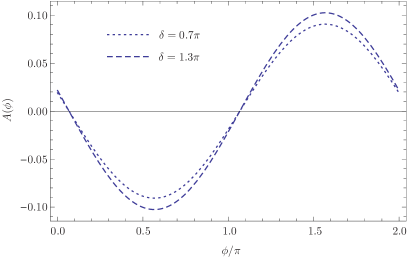
PDG data		CLAS Collaboration data

Figure 10: The charge asymmetry $A$ as a function of the relative phase $\phi$ for different values of the phase $\delta$.

It is seen that the charge asymmetry in the $e^{+}e^{-}\to\eta\pi^{+}\pi^{-}$ process may be quite large, up to $\pm 10\%$ for $\phi\simeq\mp\pi/2$.

VIII Conclusion

We calculate the width of the $f_{1}(1285)\to e^{+}e^{-}$ decay in the vector meson dominance model, where both virtual photons are coupled with the $f_{1}$ meson via the intermediate $\rho^{0}$ mesons; see Fig. 3. We assume that this is the main mechanism of the decay, and such an assumption is based on the experimental data on $f_{1}\to 4\pi$ and $f_{1}\to\rho^{0}\gamma$ decays Barberis:00 ; pdg16 . In our model the decay width, $\Gamma(f_{1}\to e^{+}e^{-})$, depends on the relative phase $\delta$ between two coupling constants describing the $f_{1}\to\rho^{0}\gamma$ decay. This phase is not fixed unambiguously from the experimental data. Therefore, the width can only be estimated as $\Gamma(f_{1}\to e^{+}e^{-})\simeq 0.07\textendash 0.19$ eV using the PDG data pdg16 , and as $\Gamma^{CLAS}(f_{1}\to e^{+}e^{-})\simeq 0.07\textendash 0.10$ eV using the CLAS Collaboration data Dickson:16 . The corresponding branching ratio is $\mathcal{B}(f_{1}\to e^{+}e^{-})\simeq(3\textendash 8)\cdot 10^{-9}$ and $\mathcal{B}^{CLAS}(f_{1}\to e^{+}e^{-})\simeq(4\textendash 5)\cdot 10^{-9}$.

The process of direct $f_{1}$ production in $e^{+}e^{-}$ collisions, $e^{+}e^{-}\to f_{1}\to mesons$, is still not measured due to smallness of the corresponding cross section. Now it can be studied at modern high-luminosity colliders, e.g., at VEPP-2000 in Novosibirsk. We estimate the $e^{+}e^{-}\to f_{1}\to\eta\pi\pi$ cross section and find it to be $\sigma(e^{+}e^{-}\to f_{1}\to a_{0}^{\pm}\pi^{\mp}\to\eta\pi^{+}\pi^{-})\simeq 5.2\textendash 20\ {\rm pb}$ ($\sigma^{CLAS}\simeq 7\textendash 13.3\ {\rm pb}$) for the $\eta\pi^{+}\pi^{-}$ final state, and $\sigma(e^{+}e^{-}\to f_{1}\to a_{0}^{0}\pi^{0}\to\eta\pi^{0}\pi^{0})\simeq 2.6\textendash 10\ {\rm pb}$ ($\sigma^{CLAS}\simeq 3.5\textendash 6.7\ {\rm pb}$) for the $\eta\pi^{0}\pi^{0}$ final state. The latter process, $e^{+}e^{-}\to f_{1}\to\eta\pi^{0}\pi^{0}$, is more convenient to study, because the $e^{+}e^{-}\to\eta\pi^{0}\pi^{0}$ reaction proceeds only through two-photon annihilation. Therefore, there is no background from one-photon annihilation, and the $e^{+}e^{-}\to f_{1}\to\eta\pi^{0}\pi^{0}$ cross section can be measured directly. In our model the lower bound on this cross section is quite small, $\sim 3$ pb. However, even such a small cross section can be measured in a special experiment at the VEPP-2000 $e^{+}e^{-}$ collider in Novosibirsk.

In contrast, the reaction $e^{+}e^{-}\to\eta\pi^{+}\pi^{-}$ proceeds mainly through one-photon annihilation. Therefore, measurement of the cross section of the two-photon channel, $e^{+}e^{-}\to f_{1}\to\eta\pi^{+}\pi^{-}$, is a rather complicated task, because of the background from one-photon annihilation. One possibility to overcome this difficulty is to investigate the charge asymmetry which arises from the interference of $C$-odd one-photon and $C$-even two-photon amplitudes. We calculate this asymmetry in the $e^{+}e^{-}\to\eta\pi^{+}\pi^{-}$ reaction for some values of parameters in our model. It turns out that the magnitude of the charge asymmetry is quite uncertain. It depends on the relative phase $\phi$ and may be quite large, up to $\pm 10\%$.

We hope that in the nearest future our predictions will be tested in precise experiments at $e^{+}e^{-}$ colliders. Such experiments could allow us to obtain values of free parameters of our model, $\delta$ and $\phi$, as well as to define more accurately $\mathcal{B}(f_{1}\to\rho^{0}\gamma)$, $\Gamma_{f}$, and $r$, measured by now with quite large uncertainties.

Acknowledgments

I am grateful to V.P. Druzhinin and A.I. Milstein for the constant interest and numerous valuable remarks and suggestions. I also thank A.L. Feldman, L.V. Kardapoltsev, M.G. Kozlov, and D.V. Matvienko for the useful discussions. This work is partly supported by the Grant of President of Russian Federation for the leading scientific Schools of Russian Federation, NSh-9022-2016.2.

References

(1)
G. Altarelli, S. De Gennaro, E. Celeghini, G. Longhi, and R. Gatto,
Theoretical calculations for electron-positron colliding-beam reactions,
Nuovo Cim. A 47 (1967) 113.
(2)
A.I. Vainshtein and I.B. Khriplovich,
On the possibility of studying resonances with positive charge parity in colliding electron-positron beams (in Russian),
Yad. Fiz. 13 (1971) 620.
(3)
M.N. Achasov et al. (SND Collaboration),
Search for the decay with the SND detector,
Phys. Rev. D 91 (2015) 092010 [arXiv:1504.01245].
(4)
R.R. Akhmetshin et al. (CMD-3 Collaboration),
Search for the process with the CMD-3 detector,
Phys. Lett. B 740 (2015) 273 [arXiv:1409.1664].
(5)
M.N. Achasov et al. (SND Collaboration),
Search for direct production of and mesons in annihilation,
Phys. Lett. B 492 (2000) 8 [hep-ex/0009048].
(6)
M. Ablikim et al. (BESIII Collaboration),
An improved limit for of and measurement of ,
Phys. Lett. B 749 (2015) 414 [arXiv:1505.02559].
(7)
J. Kaplan and J.H. Kühn,
Direct production of states in annihilation,
Phys. Lett. B 78 (1978) 252.
(8)
J.H. Kühn, J. Kaplan, and E.G.O. Safiani,
Electromagnetic annihilation of into quarkonium states with even charge conjugation,
Nucl. Phys. B 157 (1979) 125.
(9)
A. Denig, F-K. Guo, C. Hanhart, and A.V. Nefediev,
Direct production in collisions,
Phys. Lett. B 736 (2014) 221 [arXiv:1405.3404].
(10)
H. Czyz, J.H. Kühn, and S. Tracz,
and production at colliders,
Phys. Rev. D 94 (2016) 034033 [arXiv:1605.06803].
(11)
H. Czyz and P. Kisza,
Testing properties at BELLE II,
Phys. Lett. B 771 (2017) 487 [arXiv:1612.07509].
(12)
N. Kivel and M. Vanderhaeghen,
decays revisited,
JHEP 1602 (2016) 032 [arXiv:1509.07375].
(13)
G. Köpp, T.F. Walsh, and P. Zerwas,
Hadron production in virtual photon-photon annihilation,
Nucl. Phys. B 70 (1974) 461.
(14)
F.M. Renard,
resonances in collisions,
Nuovo Cim. A 80 (1984) 1.
(15)
R.N. Cahn,
Production of spin 1 resonances in collisions,
Phys. Rev. D 35 (1987) 3342;
R.N. Cahn,
Cross-sections for single tagged two photon production of resonances,
Phys. Rev. D 37 (1988) 833.
(16)
G.A. Schuler, F.A. Berends, and R. van Gulik,
Meson photon transition form-factors and resonance cross-sections in collisions,
Nucl. Phys. B 523 (1998) 423 [hep-ph/9710462].
(17)
G. Gidal et al. (Mark II Collaboration),
Observation of spin-1 in the reaction ,
Phys. Rev. Lett. 59 (1987) 2012.
(18)
H. Aihara et al. (TPC/2 Collaboration),
formation in photon photon fusion reactions,
Phys. Lett. B 209 (1988) 107;
H. Aihara et al. (TPC/2 Collaboration),
Formation of spin one mesons by photon-photon fusion,
Phys. Rev. D 38 (1988) 1.
(19)
P. Achard et al. (L3 Collaboration),
formation in two photon collisions at LEP,
Phys. Lett. B 526 (2002) 269 [hep-ex/0110073].
(20)
D. Yang and S. Zhao,
within and beyond the Standard Model,
Eur. Phys. J. C 72 (2012) 1996 [arXiv:1203.3389].
(21)
C. Patrignani et al. (Particle Data Group),
Review of particle physics, Chin. Phys. C 40 (2016) no. 10, 100001.
(22)
L.D. Landau,
On the angular momentum of a system of two photons,
Dokl. Akad. Nauk USSR Ser. Fiz. 60 (1948) 207
[Collected Papers of L.D. Landau (Elsevier, Amsterdam, 1965), p. 471];
C.N. Yang,
Selection rules for the dematerialization of a particle into two photons,
Phys. Rev. 77 (1950) 242.
(23)
D. Barberis et al. (WA102 Collaboration),
A spin analysis of the channels produced in central pp interactions at 450 GeV/c,
Phys. Lett. B 471 (2000) 440 [hep-ex/9912005].
(24)
D.V. Amelin et al. (VES Collaboration),
Study of the decay ,
Z. Phys. C 66 (1995) 71.
(25)
R. Dickson et al. (CLAS Collaboration),
Photoproduction of the meson,
Phys. Rev. C 93 (2016) 065202 [arXiv:1604.07425].
(26)
N.I. Kochelev, M. Battaglieri, and R. De Vita,
Exclusive photoproduction of meson off the proton in kinematics
available at the Jefferson Laboratory experimental facilities,
Phys. Rev. C 80 (2009) 025201 [arXiv:0903.5369].
(27)
Y.Y. Wang, L.J. Liu, E. Wang, and D.M. Li,
Study on the reaction of in Regge-effective Lagrangian approach,
Phys. Rev. D 95 (2017) 096015 [arXiv:1701.06007].
(28)
X.Y. Wang and J. He,
Analysis of recent CLAS data on photoproduction,
Phys. Rev. D 95 (2017) 094005 [arXiv:1702.06848].
(29)
A.A. Osipov, A.A. Pivovarov, and M.K. Volkov,
Anomalous decay and related processes,
Phys. Rev. D 96 (2017) 054012 [arXiv:1705.05711].
(30)
M.F.M. Lutz and S. Leupold,
On the radiative decays of light vector and axial-vector mesons,
Nucl. Phys. A 813 (2008) 96 [arXiv:0801.3821].
(31)
V.M. Aulchenko et al. (SND Collaboration),
Measurement of the cross section in the center-of-mass energy range 1.22-2.00 GeV with the SND detector at the VEPP-2000 collider,
Phys. Rev. D 91 (2015) 052013 [arXiv:1412.1971].
(32)
N.N. Achasov and V.A. Karnakov,
On the research of the reaction,
Pis’ma Zh. Eksp. Teor. Fiz. 39 (1984) 285 [JETP Lett. 39 (1984) 342].