Rare events and discontinuous percolation transitions

Abstract

Percolation theory characterizing the robustness of a network has applications ranging from biology, to epidemic spreading, and complex infrastructures. Percolation theory, however, only concern the typical response of an infinite network to random damage of its nodes while in real finite networks, fluctuations are observable. Consequently for finite networks there is an urgent need to evaluate the risk of collapse in response to rare configurations of the initial damage. Here we build a large deviation theory of percolation characterizing the response of a sparse network to rare events. This general theory includes the second order phase transition observed typically for random configurations of the initial damage but reveals also discontinuous transitions corresponding to rare configurations of the initial damage for which the size of the giant component is suppressed.

I Introduction

Percolation theory crit ; Kahng_review ; Newman_old1 ; Laszlo_robustness ; Cohen1 ; Cohen2 plays a pivotal role in characterizing the robustness of a network as it sheds light on the fundamental structural properties that determine its response when a fraction of nodes is initially damaged. Therefore percolation theory is a fundamental critical phenomena that permeates statistical mechanics as well as network science NS ; Newman_book ; Havlin_book having profound implications in different contexts ranging from ecological networks to infrastructures.

Despite the fact that the percolation transition is second order, cascade of failure events that abruptly dismantle a network are actually occurring in real systems, with major examples ranging from large electric blackouts to the sudden collapse of ecological systems. In order to explain how abrupt phase transitions could result from percolation, recently generalized percolation problems including percolation in interdependent multilayer networks Havlin1 ; Doro_multiplex ; Son ; Redundant ; Cellai2013 ; Radicchi ; Havlin2 , and explosive percolation Explosive ; Doro_explosive ; Riordan_explosive ; Grassberger_explosive that retards the percolation transition, have been proposed. It has been shown that in interdependent multilayer networks discontinuous phase transitions are the rule Havlin1 ; Doro_multiplex ; Son ; Redundant ; Cellai2013 ; Radicchi ; Havlin2 . For explosive percolation it has been proved that the original Achiloptas process Explosive ; Doro_explosive ; Riordan_explosive ; Grassberger_explosive yields a steep but continuous transition despite some of its modifications are currently believed to yield genuinely discontinuous transitions Herrmann ; Kahng ; Souza . It is to note that this interest on discontinous percolation transitions has triggered further research in the statistical mechanics of networks. In fact discontinuous phase transitions have been observed also in explosive synchronization of single and multilayer networks Arenas ; Vito ; Boccaletti in the wider context of the Kuramoto dynamics previously believed to yield exclusively second order transitions.

Simple node percolation Newman_old1 ; Laszlo_robustness ; Cohen1 ; Cohen2 has been one of the most investigated critical phenomena on networks. It determines the response of the network to a random initial damage. Since belonging to the giant component is often considered a pre-requisit for the node to be functional, all the nodes that are not any more in the giant component are assumed to fail as a consequence of the initial damage. Therefore characterizing the percolation transition on a single network is widely considered as a simple yet powerful way to evaluate the robustness of a network. Despite recently some attention has been drawn to the characterization of extremal configurations of the initial damage that dismantle most efficiently complex networks Makse ; Dismantling ; Fluct1 , the vast majority of the scientific research concerns so far the typical scenario characterized by the well known continous second order phase transition Newman_old1 ; Laszlo_robustness ; Cohen1 ; Cohen2 .

In infinite networks percolation is known to be self-averaging, i.e. fluctuations from the typical behavior are vanishing. However in finite real networks rare events are observable and it is of fundamental importance to have a complete theoretical framework for characterizing the response of the network also to rare configurations of the initial damage. Here we address this problem by investigating the large deviations Touchette of percolation on sparse networks. We show that percolation theory on single networks includes both continuous and discontinuous phase transitions as long as we consider also rare events. The entire phase diagram of percolation is uncovered using naturally defined thermodynamic quantities including the free energy, the entropy and the specific heat of percolation. The continuous phase transition dominating the typical behavior is derived in the context of this more general theoretical approach. Additionally we observe that rare configurations of the damage yield discontinuous phase transitions whereas the imposed bias on the configurations of the initial damage tends to suppress the size of the giant component. These results shed new light on possible mechanisms yielding abrupt phase transitions ecosystems and might play a crucial role for determining early warning signals of these transitions. Using the theory of large deviations we show that the observed discontinuous phase transitions are caused by the fact that particularly damaging initial damage configurations can be observable in finite networks.

It is well known that the percolation transition can be studied by investigating the Potts model in the limit in which the spins can be in $q\to 1$ states FK ; Wu . Interestingly the Potts formalism has been also used to explore the large deviation of the number of clusters in random and complex networks Monasson ; Bradde . Our approach is rather distinct from these previous studies because we are not concerned with the probability of observing a certain number of clusters, but instead we focus on the probability of the initial damage configurations that yield a given size of the giant component. We note here that while the number of clusters does not determine the properties of the percolation transition, the size of the giant component is nothing else that the order parameter of percolation and therefore it is the key quantity determining the transition.

Our approach, based on a locally tree-like approximation, uses a message passing algorithm, specifically Belief Propagation Mezard ; Weigt ; Yedida ; Semerjian . Message passing algorithms are becoming increasingly relevant in the context of complex networks and have been recently widely used for percolation Cellai2013 ; Radicchi ; Lenka , epidemic spreading Epidemics_Luca ; Saad ; Gleeson_MP and network control Control ; Bianconi_control . The proposed Belief Propagation algorithm reveals the large deviation of percolation and characterizes its phase diagram on single network realizations including real network datasets and single instances of random network ensembles. Here we apply this theoretical framework both to real datasets of foodwebs and to uncorrelated network ensembles.

The paper is organized as follows: in Sec. II we describe the large deviation approach to percolation, in Sec. III we provide the detailed Belief Propagation equations that solve the large deviation properties of percolation on single networks, in Sec. IV we characterize the equations determining the large deviation of percolation in network ensembles. In Sec. V we provide analytical evidence of the discontinuous phase transition observed for regular networks as soon as the giant component is suppressed and we study the large deviation properties of percolation on Poisson networks and real foodwebs using the BP algorithm. Finally in Sec VI we provide the conclusions.

II The large deviation approach to percolation

II.1 Message passing algorithm on single realization of damage

Let us consider a given locally tree-like network of $N$ nodes where each node $i=1,2,\ldots,N$ is either damaged ($x_{i}=0$) or not ($x_{i}=1$). In this case it is well known that the following message passing algorithm is able to determine whether a node belongs ($\rho_{i}=1$) or not ($\rho_{i}=0$) to the giant component. Specifically the message passing algorithm consists on a set or recursive equations written for the messages $\sigma_{i\to j}$ that each node $i$ send to a neighbour node $j$ of the network. (Note that of each interaction between node $i$ and node $j$ there are two distinct messages $\sigma_{i\to j}$ and $\sigma_{j\to i}$). The message passing equations read,

$$\sigma_{i\to j}=x_{i}\left[1-\prod_{\ell\in N(i)\setminus j}(1-\sigma_{\ell\to i})\right],$$ (1)

where $N(i)$ indicates the set of neighbours of node $i$. The messages $\sigma_{i\to j}$ that $\rho_{i}$ which is given by

$$\rho_{i}=x_{i}\left[1-\prod_{j\in N(i)}(1-\sigma_{j\to i})\right].$$ (2)

Finally the size of the giant component of the network ${\mathcal{R}}$, resulting after the inflicted initial damage $\{x_{i}\}_{i=1,2,\ldots,N}$ is given by

$${\mathcal{R}}=\sum_{i=1}^{N}\rho_{i}.$$ (3)

Therefore different realizations of the initial damage can yield, in general, giant components of different sizes (see schematic discussion in Figure 1).

In the following we will indicate with $\bm{\sigma}$ the set of all the messages and with $\bm{\sigma}_{i}$ the set of all the messages starting or ending at node $i$, i.e.

$$\bm{\sigma} = \{\sigma_{i\to j}\}_{i\in\{1,2,\ldots,N\};j\in N(i)},$$

$$\bm{\sigma}_{i} = \{\sigma_{i\to j},\sigma_{j\to i}\}_{j\in N(i)}.$$ (4)

Additionally we will indicate with $\bm{x}$ the configuration of the initial damage, i.e.

$$\bm{x}=\{x_{i}\}_{i\in\{1,2,\ldots,N\}}.$$ (5)

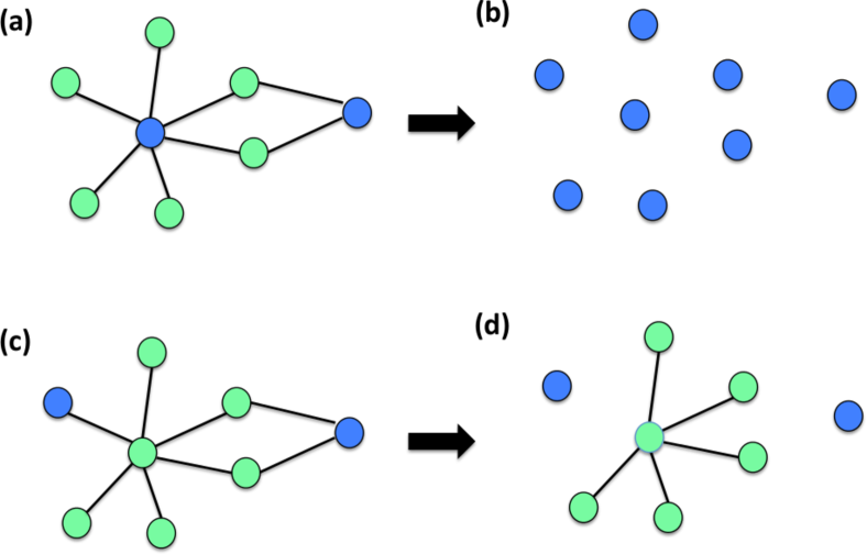
Figure 1: Different realizations of the initial damage are here shown to be more or less damaging for a network. Panel (a) shows an initial damage of a connected network affecting exclusively two out of the $N=8$ nodes of the network (blue nodes indicate damaged nodes green nodes indicate not damaged nodes). Panel (b) shows that this initial damage is very disruptive for the network and results in giant component of size $R=1$. Panel (c) shows another initial damage configuration of the same network which affects only two nodes of network. In this case panel (d) shows that the effect of the damage are reduced and most of the network remains connected resulting in a giant component $R=6$.

II.2 Random realization of the damage and typical behaviour

Here we are concerned with realizations of the initial damage $\bm{x}$ where each node is damaged with probability $1-p$, i.e. each configuration $\bm{x}$ is drawn from a distribution

$$\tilde{P}(\bm{x})=\prod_{i=1}^{N}p^{x_{i}}(1-p)^{1-x_{i}}.$$ (6)

Usually, in order to predict the expected size of the giant component $\hat{R}$ given by

$$\hat{R}=\sum_{\bm{x}}\tilde{P}(\bm{x}){\mathcal{R}},$$ (7)

the original message passing algorithm is averaged over the distribution $\tilde{P}(\bm{x})$. Given the locally tree-like structure of the network this procedure generates a novel message passing algorithm determined by the set of messages

$$\hat{\sigma}_{i\to j}=\sum_{\bm{x}}\tilde{P}(\bm{x})\sigma_{i\to j},$$ (8)

satisfying

$$\hat{\sigma}_{i\to j}=p\left[1-\prod_{\ell\in N(i)\setminus j}(1-\hat{\sigma}_{\ell\to i})\right].$$ (9)

These messages determine the probability

$$\hat{\rho}_{i}=\sum_{\bm{x}}\tilde{P}(\bm{x})\rho_{i}$$ (10)

that node $i$ is in the giant component, which is given by

$$\hat{\rho_{i}}=p\left[1-\prod_{\ell\in N(i)}(1-\hat{\sigma}_{\ell\to i})\right].$$ (11)

Finally the expected size of the giant component $\hat{R}$ is given by

$$\hat{R}=\sum_{i=1}^{N}\hat{\rho}_{i}.$$ (12)

II.3 Large deviations of percolation

Here we are interested in going beyond the typical scenario by characterizing the probability $\pi(R)$ that a given configuration of the initial damage yields a giant component of size $R$, i.e.

$$\pi(R)=\sum_{\bm{x}}\tilde{P}(\bm{x})\delta({\mathcal{R}},R),$$ (13)

where $\delta(m,n)$ is the Kronecker delta. For any given value of $p$, and for large network sizes $N\gg 1$ the probability $\pi(R)$ will follow the large deviation scaling Touchette

$$\pi({R})\sim e^{-NI({R})},$$ (14)

where $I(R)\geq 0$ is called the rate function. This expression indicates that for any given value of $p$ the deviations from the most likely size of the giant component are exponentially suppressed. Additionally this expression implies that on an infinite network the percolation transition is self-averaging and that all networks with yield almost surely the same giant component $R=\hat{R}$ for which $I(R)$ takes its minimum value $I(\hat{R})$. In order to find $I(R)$ let us introduce the partition function $Z=Z(\omega)$

$$Z = \sum_{\bm{x}}\tilde{P}(\bm{x})e^{-\omega{\mathcal{R}}}.$$ (15)

Using the definition of $\pi(R)$ given by Eq. $(\ref{pi_def})$ it can be easily shown that $Z$ is the generating function of $\pi(R)$ as $Z$ can be written as

$$Z=\sum_{R}\pi({R})e^{-\omega{R}}$$ (16)

By indicating with $F$ the corresponding free-energy and with $f$ the free energy density given by

$$\omega F=\omega Nf=-\log(Z).$$ (17)

it is immediate to show that $\omega f(\omega)$ a is the Legendre-Fenchel tranforms of the rate function $I(R)$ Touchette . In particular we have that $\omega f(\omega)$ can be expressed as

$$\omega f(\omega) = \inf_{R}\left[I(R)+\omega\frac{R}{N}\right].$$ (18)

Additionally as long $\omega f(\omega)$ is differentiable, the Legendre-Fenchel transform of $\omega f(\omega)$ fully determines $I(R)$, given by the convex function

$$I(R)=\sup_{\omega}\left[\omega f(\omega)-\omega\frac{R}{N}\right]$$ (19)

Therefore as long as $\omega f(\omega)$ is differentiable, by studying the free energy $\omega f(\omega)$ of the percolation problem the large deviation of the size of the giant component can be fully established and the rate function $I(R)$ is convex. However when $I(R)$ is non-convex $\omega f(\omega)$ is not differentiable and the Legendre-Fenchel transform of $\omega f(\omega)$ only provides the convex envelop of $I(R)$ Touchette .

II.4 The Gibbs measure over messages

In order to study the partition function $Z$, we make a change of variables and instead of considering a Gibbs measure over configurations of the initial damage we consider the Gibbs measure $P(\bm{\sigma})$ over the set $\bm{\sigma}$ of all messages. The probability $P(\bm{\sigma})$ allows us to determine the most likely distribution of the messages corresponding to a given size of the giant component ${\mathcal{R}}$. The large deviations properties of percolation are studied by introducing a Lagrangian multiplier $\omega$ modulating the average size of the giant component ${\mathcal{R}}$.Therefore the Gibbs measure $P(\bm{\sigma})$ is given by

$$P({\bm{\sigma}})=\frac{1}{Z}\sum_{{\bm{x}}}e^{-\omega{\mathcal{R}}}\tilde{P}({\bf x})\chi(\bm{\sigma},\bm{x}),$$ (20)

where the function $\chi(\bm{\sigma},\bm{x})$ enforces the message passing Eqs. $(\ref{mess})$, i.e.

$$\chi(\bm{\sigma},\bm{x})=\prod_{i=1}^{N}\prod_{j\in N(i)}\delta\left(\sigma_{i\to j},x_{i}\left[1-\prod_{\ell\in N(i)}(1-\sigma_{\ell\to i})\right]\right).$$

Here $Z$ is the partition function of the problem and it can be easily shown that it reduces to $Z$ defined in Eq. (16), i.e.

$$Z=\sum_{\bm{\sigma}}\sum_{{\bm{x}}}e^{-\omega{\mathcal{R}}}\tilde{P}({\bm{x}})\chi({\bm{x}},\bm{\sigma})=\sum_{R}\pi(R)e^{-\omega{R}}.$$ (21)

The role of $\omega$ in determining the Gibbs measure $P(\bm{\sigma})$ is equivalent to the one of temperature in a canonical ensemble. Since for each node only two options are possible: either a node belongs $(\rho_{i}=1)$ or do not ($\rho_{i}=0$) belong to the giant component, this problem can be interpreted as a statistical mechanics problem of a two level systems. Therefore it is possible to investigate the role of both positive and negative values of $\omega$.

For $\omega<0$, the Gibbs measure weights more the buffering configurations of the initial damage resulting in a giant component larger than the typical one. On the contrary for $\omega>0$ the Gibbs measure weights more the aggravating configurations of the initial damage resulting in a giant component smaller than the typical one. For $\omega=0$ we recover the typical scenario.

From Eq. $(\ref{Pss})$ it follows that $P(\bm{\sigma})$ can be expressed as

$$P(\bm{\sigma})=\frac{1}{Z}\prod_{i=1}^{N}\psi_{i}(\bm{\sigma}_{i},\omega),$$ (22)

where the set of constraints $\psi_{i}(\bm{\sigma}_{i},\omega)$ for $i=1,2,\ldots,N$ defined over all the messages $\bm{\sigma}_{i}$ starting or ending to node $i$ read

$$\psi_{i}(\bm{\sigma}_{i}) = \left[(1-p)\prod_{j\in N(i)}\delta(\sigma_{i\to j},0)\right.$$ (23)

$$+\left.pe^{-\omega\hat{\rho_{i}}}\prod_{j\in N(i)}\delta\left(\sigma_{i\to j},1-\prod_{\ell\in N(i)\setminus j}(1-\sigma_{\ell\to i})\right)\right],$$

where $\delta(m,n)$ indicates the Kronecker delta and $\hat{\rho}_{i}$ is given by

$$\hat{\rho_{i}}=\left[1-\prod_{j\in N(i)}(1-\sigma_{j\to i})\right].$$ (24)

Given Eq. $(\ref{GM})$ it follows that the partition function $Z$ can be also written as

$$Z=\sum_{\bm{\sigma}}\prod_{i=1}^{N}\psi_{i}(\bm{\sigma}_{i},\omega).$$ (25)

From this theoretical framework it is possible to derive naturally the following thermodynamic quantities for percolation: energy $R$, free energy $F$, entropy $S$ and specific heat $C$. Specifically the energy $R$ is the average size of the giant component of the network, the free energy $F$ is proportional to the logarithm of the partition function $Z$ with $\omega F(\omega)/N$ indicating the Legendre-Fenchel transform of the rate function $I(R)$, the entropy $S$ determines the logarithm of the typical number of message configurations that yield a given size of the giant component $R$ and the specific heat $C$ is proportional to the variance of the giant component for given values of $p$ and $\omega$ (see Table 1).

Thermodynamic quantities	Mathematical relations
Energy $R$	$R=-\frac{\partial\ln Z}{\partial\omega}$
Free energy $F$	$\omega F=-\ln Z$
Entropy $S$	$S=-\sum_{\bm{\sigma}}P(\bm{\sigma})\ln P(\bm{\sigma})$
Specific heat $C$	$C=\omega^{2}\frac{\partial^{2}\ln Z}{\partial\omega^{2}}$

Table 1: The thermodynamic quantities of percolation (energy $R$, free energy $F$, entropy $S$ and specific heat $C$) are listed together with their mathematical expression in terms of the probability $P(\bm{\sigma})$ and its associated partition function $Z$.

The Gibbs measure and the corresponding thermodynamic quantities can be calculated in the locally tree-like approximation using Belief Propagation (BP) for any given locally tree-like network, representing either a real network dataset or a single instance of a random network model. Moreover the BP equations can be also averaged over network ensembles with degree distribution $P(k)$ characterizing the nature of the phase transition (see next two sections).

III Large deviation theory of percolation on single networks

III.0.1 The Belief Propagation equations

The Gibbs distribution $P(\bm{\sigma})$ can be expressed explicitly on a locally tree-like network using the Belief Propagation (BP) method Mezard ; Yedida ; Weigt ; Semerjian by finding the messages $\hat{P}_{i\to j}(\sigma_{i\to j},\sigma_{j\to i})$ that each node $i$ sends to the generic neighbour node $j$. These message satisfy the following recursive BP equations

$$\hat{P}_{i\to j}(\sigma_{i\to j},\sigma_{j\to i})=\frac{1}{{\mathcal{C}}_{i\to j}}\sum_{\bm{\sigma}_{i}}\psi_{i}(\bm{\sigma}_{i})\prod_{\ell\in N(i)\setminus j}\hat{P}_{\ell\to i}(\sigma_{\ell\to i},\sigma_{i\to\ell}),$$

where ${\mathcal{C}}_{i\to j}$ are normalization constants enforcing the normalization condition

$$\sum_{\sigma_{i\to j}=0,1}\sum_{\sigma_{j\to i}=0,1}\hat{P}_{i\to j}(\sigma_{i\to j},\sigma_{j\to i})=1.$$ (26)

In the Bethe approximation, valid on locally tree-like networks the probability distribution $P(\bm{\sigma})$ is given by

$$P(\bm{\sigma}) = \prod_{i=1}^{N}{\mathcal{P}}_{i}(\bm{\sigma}_{i})\left(\prod_{<i,j>}{\mathcal{P}}_{ij}(\sigma_{i\to j},\sigma_{j\to i})\right)^{-1}$$ (27)

where ${\mathcal{P}}_{i}(\bm{\sigma}_{i})$ and ${\mathcal{P}}_{ij}(\sigma_{i\to j},\sigma_{j\to i})$ indicate the marginal distribution of nodes and links and are given by

$${\mathcal{P}}_{ij}(\sigma_{i\to j},\sigma_{j\to i}) = \frac{1}{\mathcal{C}_{ij}}\hat{P}_{i\to j}(\sigma_{i\to j},\sigma_{j\to i})\hat{P}_{j\to i}(\sigma_{j\to i},\sigma_{i\to j}),$$

$${\mathcal{P}}_{i}(\bm{\sigma}_{i}) = \frac{1}{\mathcal{C}_{i}}\psi_{i}(\bm{\sigma}_{i})\prod_{j\in N(i)}\hat{P}_{j\to i}(\sigma_{j\to i},\sigma_{i\to j}),$$ (28)

with ${\mathcal{C}}_{i}$ and ${\mathcal{C}}_{ij}$ indicating normalization constants.The BP equations can be written explicitly as

$${\hat{P}}_{i\to j}(0,0) = \frac{1}{{\mathcal{C}}_{i\to j}}\left[(1-p)\prod_{\ell\in N(i)\setminus j}[\hat{P}_{\ell\to i}(0,0)+\hat{P}_{\ell\to i}(1,0)]+p\prod_{\ell\in N(i)\setminus j}\hat{P}_{\ell\to i}(0,0)\right]$$

$$\hat{P}_{i\to j}(0,1) = \frac{1}{{\mathcal{C}}_{i\to j}}\left[(1-p)\prod_{\ell\in N(i)\setminus j}[\hat{P}_{\ell\to i}(0,0)+\hat{P}_{\ell\to i}(1,0)]+pe^{-\omega}\prod_{\ell\in N(i)\setminus j}\hat{P}_{\ell\to i}(0,1)\right]$$

$$\hat{P}_{i\to j}(1,1) = \frac{1}{{\mathcal{C}}_{i\to j}}pe^{-\omega}\left[\prod_{\ell\in N(i)\setminus j}[\hat{P}_{\ell\to i}(0,1)+\hat{P}_{\ell\to i}(1,1)]-\prod_{\ell\in N(i)\setminus j}\hat{P}_{\ell\to i}(0,1)\right]$$

$$\hat{P}_{i\to j}(1,0) = \frac{1}{{\mathcal{C}}_{i\to j}}pe^{-\omega}\left\{\sum_{\ell\in N(i)}\hat{P}_{\ell\to i}(1,0)\prod_{\ell^{\prime}\in N(i)\setminus j,\ell}\hat{P}_{\ell^{\prime}\to i}(0,1)\right.$$ (29)

$$\left.+\prod_{\ell\in N(i)\setminus j}\left[\hat{P}_{\ell\to i}(0,1)+P_{\ell\to i}(1,1)\right]-\prod_{\ell\in N(i)\setminus j}\hat{P}_{\ell\to i}(0,1)-\sum_{\ell\in N(i)}\hat{P}_{\ell\to i}(1,1)\prod_{\ell^{\prime}\in N(i)\setminus j}\hat{P}_{\ell\to i}(0,1)\right\},$$

if the degree $k_{i}$ of node $i$ is greater than one (i.e. $k_{i}>1)$, whereas if the degree of node $i$ is one ($k_{i}=1$), the messages are given by $\hat{P}_{i\to j}(0,0)=\hat{P}_{i\to j}(0,1)=1/2$ and $\hat{P}_{i\to j}(1,0)=\hat{P}_{i\to j}(1,1)=0$.

By solving this set of recursive equations on a given single network realization, using Eqs. $(\ref{uno})$, $(\ref{marginals})$ and $(\ref{BPe})$ it is therefore possible to determine the distribution $P(\bm{\sigma})$ in the Bethe approximation as long as the network is locally tree-like.

III.0.2 Free energy

The free energy of the problem can be found by minimizing the Gibbs free energy $F$ given by

$$\omega F=\sum_{\bm{\sigma}}P(\bm{\sigma})\ln\left(\frac{P(\bm{\sigma})}{\psi(\bm{\sigma})}\right)$$ (30)

where $\psi(\bm{\sigma})$ indicates the constraints

$$\psi(\bm{\sigma})=\prod_{i=1}^{N}\psi_{i}(\bm{\sigma}_{i})$$ (31)

Indeed the Gibbs free energy $F$ is minimal when calculated over the probability distribution $P(\bm{\sigma})$ given by Eq. $(\ref{GM})$ when $\omega F=-\ln Z$. By considering the Bethe approximation for the distribution $P(\bm{\sigma})$ Eq. $(\ref{uno})$, it is straightforward to see that the free energy can be expressed as

$$\omega F=\sum_{<i,j>}\log({\mathcal{C}}_{ij})-\sum_{i=1}^{N}\log({\mathcal{C}}_{i})$$ (32)

where the constants ${\mathcal{C}}_{ij},{\mathcal{C}}_{i}$ can be found directly in terms of the messages $\hat{P}_{i\to j}(a,b)$, with $a,b\in\{0,1\}$. Indeed we have

$${\mathcal{C}}_{ij} = [\hat{P}_{i\to j}(0,0)\hat{P}_{j\to i}(0,0)+\hat{P}_{i\to j}(0,1)\hat{P}_{j\to i}(1,0)+\hat{P}_{j\to i}(1,0)\hat{P}_{j\to i}(0,1)+\hat{P}_{i\to j}(1,1)\hat{P}_{j\to i}(1,1)],$$

$${\mathcal{C}}_{i} = (1-p)\prod_{\ell\in N(i)}[\hat{P}_{\ell\to i}(0,0)+\hat{P}_{\ell\to i}(1,0)]+p\prod_{\ell\in N(i)}\hat{P}_{\ell\to i}(0.0)+pe^{-\omega}\left\{\sum_{\ell\in N(i)}\hat{P}_{\ell\to i}(1,0)\prod_{\ell^{\prime}\in N(i)\setminus\ell}\hat{P}_{\ell^{\prime}\to i}(0,1)+\right.$$ (33)

$$\left.+\prod_{\ell\in N(i)}\left[\hat{P}_{\ell\to i}(0,1)+\hat{P}_{\ell\to i}(1,1)\right]-\prod_{\ell\in N(i)}\hat{P}_{\ell\to i}(0,1)-\sum_{\ell\in N(i)}\hat{P}_{\ell\to i}(1,1)\prod_{\ell^{\prime}\in N(i)}\hat{P}_{\ell\to i}(0,1)\right\}.$$

III.0.3 Energy and Specific Heat

The role of the energy is played by the average size of the giant component $R$ given by

$$R = \sum_{\bm{\sigma}}{\mathcal{R}}P(\bm{\sigma})=-\frac{\partial\ln Z}{\partial\omega}.$$ (34)

By solving the BP equations and calculating $R$ it is possible to observe that the system undergoes a phase transition from a non percolating phase where $R=0$ to a percolating phase where $R>0$. The set of critical points in which the transition occur is indicated by the values $(\omega_{c},p_{c})$ of the parameters $\omega$ and $p$.

The specific heat $C$ is naturally defined as

$$\frac{C}{\omega^{2}} = -\frac{\partial R}{\partial\omega}.$$

where this quantity has the explicit interpretation as the variance in the size of giant component, i.e.

$$\frac{C}{\omega^{2}}=\left(\sum_{\bm{\sigma}}{\mathcal{R}}^{2}P(\bm{\sigma})\right)-\left(\sum_{\bm{\sigma}}{\mathcal{R}}P(\bm{\sigma})\right)^{2}.$$

Both $R$ and $C/\omega^{2}$ can be derived from the message passing algorithm. Indeed we have

$$R = \sum_{i}r_{i},$$ (36)

$$\frac{C}{\omega^{2}} = \sum_{i=1}^{N}r_{i}\left(1-r_{i}\right)$$ (37)

where

$$r_{i} = \sum_{\bm{\sigma}}\rho_{i}P(\bm{\sigma})$$ (38)

indicating the probability that node $i$ is in the giant component is given by

$$r_{i}=\frac{z_{i}}{{\mathcal{C}}_{i}}$$ (39)

with

$$z_{i}=pe^{-\omega}\left\{\prod_{\ell\in N(i)}\left[\hat{P}_{\ell\to i}(0,1)+\hat{P}_{\ell\to i}(1,1)\right]-\prod_{\ell\in N(i)}\hat{P}_{\ell\to i}(0,1)\right.$$

$$\left.+\sum_{\ell\in N(i)}\left[\hat{P}_{\ell\to i}(1,0)-\hat{P}_{\ell\to i}(1,1)\right]\prod_{\ell^{\prime}\in N(i)}\hat{P}_{\ell\to i}(0,1)\right\}.$$ (40)

Note that the quantity $C/\omega^{2}$ given by Eq. $(\ref{C})$ can be also interpreted as the fraction of nodes that given two random realizations of the initial damage are found in the giant component in one realization but not in the other. This quantity has been recently proposed Fluct1 to study the fluctuations of the giant component. Here we show that this quantity can be naturally interpreted as the variance of the giant component, and it is related to the specific heat of percolation $C$.

III.0.4 Entropy

The entropy $S$ of the distribution is given by

$$S=-\sum_{\bm{\sigma}}P(\bm{\sigma})\ln P(\bm{\sigma}),$$ (41)

where $P(\bm{\sigma})$ is given by the Gibbs measure $(\ref{GM})$. From the expression of the Gibbs measure $P(\bm{\sigma})$ it follows that the entropy is related to the free energy by the equation

$$S=\omega R+H-\omega F,$$ (42)

where

$$H=\sum_{i=1}^{N}H_{i},$$ (43)

and

$$H_{i}=-\sum_{\bm{\sigma}_{i}}{\mathcal{P}}_{i}(\bm{\sigma}_{i})\ln\left[\psi_{i}(\bm{\sigma}_{i})\right].$$ (44)

The quantity $H_{i}$ can be expressed explicitely as a function of the messages as

$$H_{i} = -\frac{(1-p)\prod_{\ell\in N(i)}[\hat{P}_{\ell\to i}(0,0)+\hat{P}_{\ell\to i}(1,0)]}{\mathcal{C}_{i}}\ln(1-p)$$ (45)

$$-\left[1-\frac{(1-p)\prod_{\ell\in N(i)}[\hat{P}_{\ell\to i}(0,0)+\hat{P}_{\ell\to i}(1,0)]}{\mathcal{C}_{i}}\right]\ln p$$

III.0.5 The typical scenario ($\omega=0$)

The BP equations corresponding to $\omega=0$ reduce to the the well known equations for the percolation transition characterizing the typical scenario. In fact the BP equations $(\ref{BPe})$ have the solution

$$\hat{P}_{i\to j}(0,0) = \hat{P}_{i\to j}(0,1),$$

$$\hat{P}_{i\to j}(1,1) = \hat{P}_{i\to j}(1,0).$$ (46)

As a function of $p$ we observe a phase transition between a non-percolating phase with $R=0$, where the solution is

$$\hat{P}_{i\to j}(0,1) = \hat{P}_{i\to j}(0,0)=1/2,$$

$$\hat{P}_{i\to j}(1,1) = \hat{P}_{i\to j}(1,0)=0,$$ (47)

and a percolating phase with $R>0$ where the solution of the BP equation is always of the type given by Eqs. $(\ref{Ro0})$ but departs from Eqs. $(\ref{R0})$. By inserting the general solution Eq.$(\ref{Ro0})$ in the BP equations, and adopting the variables

$$\hat{\sigma}_{i\to j}=\hat{P}_{i\to j}(1,1)+\hat{P}_{i\to j}(1,0),$$ (48)

we recover the well known message passing equations for the typical scenario of the percolation transition Weigt ; Lenka

$$\hat{\sigma}_{i\to j}=p\left(1-\prod_{\ell\in N(i)\j}(1-\hat{\sigma}_{\ell\to i})\right).$$ (49)

In this case the probability $r_{i}$ that a node belongs to the giant component reads

$$\hat{\rho}_{i}=p\left(1-\prod_{\ell\in N(i)}(1-\hat{\sigma}_{\ell\to i})\right).$$ (50)

The thermodynamic quantities are given by

$$R = \sum_{i=1}^{N}\hat{\rho}_{i},$$

$$\frac{C}{\omega^{2}} = \sum_{i=1}^{N}\hat{\rho}_{i}(1-\hat{\rho}_{i}),$$

$$F = 0,$$

$$S = -(1-p)\ln(1-p)-p\ln p.$$ (51)

IV Large deviation theory of percolation on random networks

IV.1 Equations on random network ensemble

The BP equations can be studied over a random network with degree distribution $P(k)$. To this end we write the equations for the average messages

$$\hat{y}_{\tau}=\overline{\hat{P}_{i\to j}(\tau)}$$ (52)

where $\tau=(a,b)$ with $a,b=0,1$ and where $\overline{\ldots}$ indicates the average over the an ensemble of random networks with degree distribution $P(k)$. Since the variables $(y_{00},y_{01},y_{11},y_{10})$ are not independent but are related by the identity

$$\hat{y}_{10}=1-y_{00}-y_{01}-y_{11},$$

the equations for the three independent variables $(y_{00},y_{01},y_{11})$ read,

$$\hat{y}_{00} = \sum_{k}\frac{k}{\left\langle{k}\right\rangle}P(k)\frac{\left[(1-p)\left(1-\hat{y}_{01}-\hat{y}_{11}\right)^{k-1}+p\hat{y}_{00}^{k-1}\right]}{d_{k}}$$

$$\hat{y}_{01} = \sum_{k}\frac{k}{\left\langle{k}\right\rangle}P(k)\frac{\left[(1-p)\left(1-\hat{y}_{01}-\hat{y}_{11}\right)^{k-1}+pe^{-\omega}\hat{y}_{01}^{k-1}\right]}{d_{k}}$$

$$\hat{y}_{11} = \sum_{k}\frac{k}{\left\langle{k}\right\rangle}P(k)\frac{pe^{-\omega}[(\hat{y}_{01}+\hat{y}_{11})^{k-1}-\hat{y}_{01}^{k-1}]}{d_{k}}$$

with $d_{k}$ given by

$$d_{k} = 2(1-p)\left(1-\hat{y}_{01}-\hat{y}_{11}\right)^{k-1}+p\hat{y}_{00}^{k-1}$$ (54)

$$+pe^{-\omega}\left\{2(\hat{y}_{01}+\hat{y}_{11})^{k-1}-\hat{y}_{01}^{k-1}\right.$$

$$\left.+(k-1)[1-y_{00}-\hat{y}_{01}-2\hat{y}_{11}]\hat{y}_{01}^{k-2}\right\}.$$

The fraction of nodes of degree $k$ that are in the giant component, $\rho_{k}$ is given by

$$\rho_{k} = \frac{z_{k}}{{\mathcal{C}}_{k}},$$ (55)

where

$$z_{k} = pe^{-\omega}\left[(\hat{y}_{01}+\hat{y}_{11})^{k}-\hat{y}_{01}^{k}\right.$$

$$\left.+k(1-\hat{y}_{00}-\hat{y}_{01}-2\hat{y}_{11})\hat{y}_{01}^{k-1}\right]$$

$${\mathcal{C}}_{k} = (1-p)(1-\hat{y}_{01}-\hat{y}_{11})^{k}+p\hat{y}_{00}^{k}+z_{k}.$$ (56)

The fraction of nodes in the giant component $r=R/N$ and the normalized specific heat $c=C/N$ are given in terms of $\rho_{k}$ as

$$r = \sum_{k}P(k)\rho_{k},$$

$$\frac{c}{\omega^{2}} = \sum_{k}P(k)\rho_{k}\left(1-\rho_{k}\right).$$ (57)

Finally the free energy density $f=F/N$ and normalized entropy $s=S/N$ are given respectively by

$$\omega f(\omega) = \frac{\langle{k}\rangle}{2}\ln\left[\hat{y}_{00}^{2}+2\hat{y}_{01}(1-\hat{y}_{00}-\hat{y}_{01}-\hat{y}_{11})+\hat{y}_{11}^{2}\right]$$

$$-\sum_{k}P(k)\ln{\mathcal{C}}_{k},$$

$$s = -\omega f(\omega)+\omega r+\sum_{k}P(k)h_{k}$$ (58)

where ${\mathcal{C}}_{k}$ is given by Eq. $(\ref{zC})$ and $h_{k}$ is given by

$$h_{k} = -(1-p)\frac{(1-\hat{y}_{01}-\hat{y}_{11})^{k}}{{\mathcal{C}}_{k}}\ln(1-p)$$ (59)

$$-\left(1-\frac{(1-p)(1-\hat{y}_{01}-\hat{y}_{11})^{k}}{{\mathcal{C}}_{k}}\right)\ln p.$$

IV.2 The transition on the random ensemble

The nature of the percolation transition can be explored by linearizing the Eqs. $(\ref{ensemble2})$ close to the solution ${\bf\hat{y}}^{\star}=(\hat{y}_{00}^{\star},\hat{y}_{01}^{\star},\hat{y}_{11}^{\star})$. In this way we get a linear system of equations that reads,

$${\bf\hat{y}}-{\bf\hat{y}}^{\star}={\bf\hat{J}}[{\bf\hat{y}}-{\bf\hat{y}^{\star}}]$$ (60)

where the $3\times 3$ Jacobian matrix ${\bf\hat{J}}$ has elements

$$\hat{J}_{\alpha,\beta}=\left.\frac{\partial\hat{y}_{\alpha}}{\partial\hat{y}_{\beta}}\right|_{{\bf\hat{y}}={\bf\hat{y}^{\star}}}.$$ (61)

with $\alpha,\beta\in\{00,01,11\}$.

This system of equations becomes unstable when the eigenvalue $\hat{\Lambda}_{\hat{J}}$ with maximum real part satisfies

$$Re[\hat{\Lambda}_{\hat{J}}]=1.$$ (62)

Therefore this is the condition determining together with Eqs. $(\ref{ensemble2})$ the percolation transition.

In the typical scenario, $\omega=0$ we get that this equation studied as a function of $p$ yield the well known continuous percolation transition describing the onset of the instability of the trivial solution ${\bf\hat{y}}^{\star}=(1/2,1/2,0)$ at

$$p\frac{\left\langle{k(k-1)}\right\rangle}{\left\langle{k}\right\rangle}=1.$$ (63)

In particular the $3\times 3$ Jacobian matrix ${\bf J}$ at ${\bf\hat{y}}^{\star}=(1/2,1/2,0)$ is given by

$${\bf J}=\left(\begin{array}[]{ccc}p\frac{\left\langle{k(k-1)}\right\rangle}{\left\langle{k}\right\rangle}&0&0\\ 0&p\frac{\left\langle{k(k-1)}\right\rangle}{\left\langle{k}\right\rangle}&0\\ 0&0&p\frac{\left\langle{k(k-1)}\right\rangle}{\left\langle{k}\right\rangle}\end{array}\right).$$ (67)

As a function of $\omega$ we have a line of critical points. These points correspond to a continuous phase transition whereas Eq. $(\ref{ensemble2})$ and Eq. $(\ref{transition})$ are satisfied at the trivial solution where $R=0$. On the contrary the transition is discontinuous and hybrid with a square root singularity when the system of equations including Eqs. $(\ref{ensemble2})$ and Eq. $(\ref{transition})$ is satisfied at a non trivial solution consistent with a non-zero size of the giant component $R>0$.

V Application to network ensemble and real networks

V.1 Analytical results on regular networks

In any given network ensemble we have shown that the proposed theoretical framework for fixed value $\omega=0$ predicts the well known second order phase transition as a function of $p$ describing the typical percolation scenario.

In order to investigate the nature of the transition for $\omega\neq 0$ we have we have numerically solved the system of equations determining the nature of the transition (equations including Eqs. $(\ref{ensemble2})$ and Eq. $(\ref{transition})$) in the specific case of a regular network where the degree distribution is given by $P(k)=\delta(k,z)$. In this way we are able to determine the phase diagram of these networks. This phase diagram reveals that $\omega=0,p=\frac{\left\langle{k}\right\rangle}{\left\langle{k(k-1)}\right\rangle},{\bf\hat{y}}^{\star}=(1/2,1/2,0)$ separates the line of continuous phase transitions from the line of discontinuous hybrid phase transitions. In Figure 2 we show the line of critical points $(\omega_{c},p_{c})$ for the percolation transition and the corresponding critical value $R_{c}$ of the size of the giant component. The value $R_{c}=0$ observed for $\omega_{c}\leq 0$ indicates a continuous phase transition while the values $R_{c}>0$ observed for $\omega_{c}>0$ clearly indicate discontinuous and hybrid phase transitions. Therefore the continuous percolation transition only characterizes the typical scenario and the configurations corresponding to $\omega<0$ but if the percolation transition is retarded ($\omega>0$) the transition becomes discontinuous.

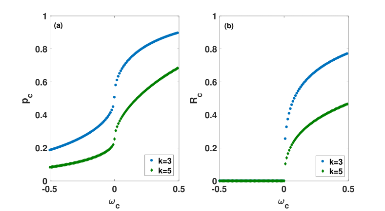
Figure 2: The line of critical points $(\omega_{c},p_{c})$ (panel (a)) and value $R_{c}$ of the size of the giant component at the transition versus $\omega_{c}$ (panel (b)) are shown for a regular network with degree distribution $P(k)=\delta(k,z)$ and $z=3$ (blue circles) and $z=5$ (green diamonds). For $\omega_{c}>0$ the transition becomes discontinuous, i. e. $R_{c}>0$.

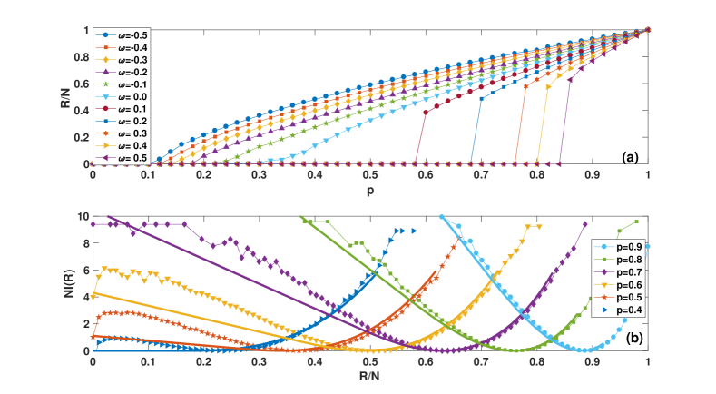
Figure 3: The large deviation of propertie of percolation in a Poisson network with $N=100$ nodes and average degree $z=3$ are here shown to include discontinuous phase transition and non-convex rate functions. Panel (a) shows the fraction of nodes in the giant component $R/N$ as a function of the probability that each node is not initially damaged $p$ for different values of $\omega$. For $\omega\leq 0$ a continuous percolation transition is observed, for $\omega>0$ a discontinuous percolation transition is observed. Panel (b) shows the rate function $I(R)$ (symbols) for different values of $p$ calculated on the same network by simulating $2\times 10^{5}$ realizations of the initial damage for each value of $p$. Solid lines in panel B represent the Legendre-Fenchel transform of $\omega F(\omega)/N$ which provides the convex envelop of the rate function $I(R)$.

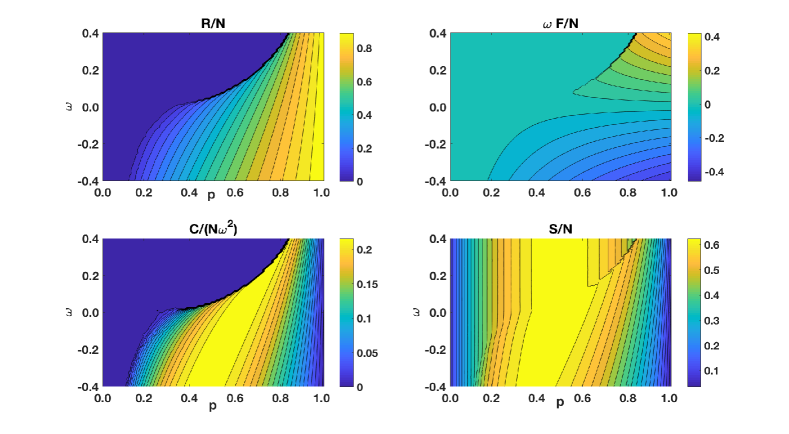
Figure 4: The phase diagram of percolation for a Poisson network with average degree $\langle{k}\rangle=3$ and $N=100$ nodes is revealed by plotting the correspodning thermodynamic properties. The thermodynamic quantities for a single realization of a Poisson network with $N=100$ nodes and average degree $\langle{k}\rangle=3$, are shown in the plane $(p,\omega)$. Here $R/N$ indicates the fraction of nodes in the giant component, $F$ indicates the free energy, $C$ indicates the specific heat with $C/\omega^{2}$ given by the variance of the size of the giant component and $S$ indicates the entropy corresponding to a given point $(p,\omega)$ of the phase diagram.

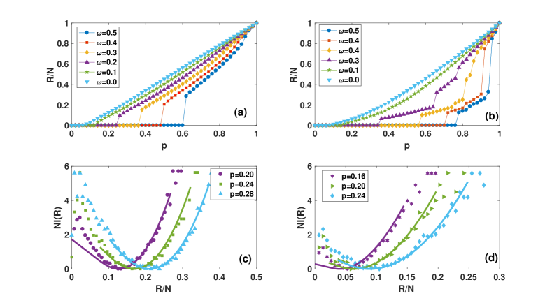
Figure 5: The size of the giant component $R$ as a function of $p$ for different values of $\omega$ is shown for the Ythan Estuary (panel (a)) and the Silwood Park (panel (b)) Foodwebs cosin . We observe that for $\omega>0$ the percolation transition is discontinuous while for $\omega=0$ we obtain the typical scenario of percolation characterized by a continuous phase transition. The non-convex rate function $I(R)$ evaluated numerically over $2\times 10^{5}$ initial realization of the random damage is shown for the Ythan Estuary (panel (c)) and the Silwood Park (panel (d)) Foodwebs and different value of $p$ (symbols). The convex envelop of $I(R)$ provided by the Legendre-Fenchel transform of $\omega F(\omega)/N$ is shown with solid lines for the same values of $p$ (note that for improving the clarity of the figure we have omitted to plot the linear part of the convex envelop for $p=0.24,0.28$ in panel (c) and for $p=0.20,0.24$ in panel (d)).

V.2 BP results on Poisson networks and real networks

All our numerical results of the BP algorithm on single sparse random networks and on real datasets suggest that the discontinuous phase transition for $\omega>0$ is observed generally. Here we consider the case of a single instance of a Poisson network on which we have run the BP algorithm. Figure 3(a) shows the predicted size of the giant component $R$ as a function of $p$ and $\omega$ for a Poisson network with $N=100$ nodes and average degree $\langle{k}\rangle=3$. For $\omega>0$ the giant component $R$ has a jump from a zero value $R=0$ to a non zero value $R>0$. Correspondingly the rate function $I(R)$ is non-convex, providing further evidence that the free energy $F$ is non-differentiable. In Figure 3(b) we show the rate function $I(R)$ evaluated numerically by simulating a large number of initial damage configurations and we compare it to the Legendre-Fenchel transform of the free energy finding very good agreement.

This investigation reveals that the observed discontinuity in the percolation problem is caused by the fact that the rate function $I(R)$ is not convex and has a local minimum for $R=0$ also when the expected typical size of the giant component takes positive values $\hat{R}>0$. Therefore the rare configuration of the damage include configurations that are damaging a finite network much more than expected typically. Moreover the observed discontinuity is an indication that these configurations of the initial damage are actually more frequent than what it might have be expected for a convex rate function.

Additionally the BP algorithm allows us to characterize the entire phase diagram of percolation using the thermodynamics quantities $R,F,C,S$ (see Figure 4) fully determining the statistical mechanics properties of the percolation transition.

Finally our theoretical approach can also be used to characterize the robustness of real datasets against rare configuration of the random damage. In Figure 5 we consider two real food webs: the Ythan Estuary (with $N=135$ nodes) and the Silwood Park (with $N=154$ nodes) Foodwebs cosin and we show numerical evidence for discontinuous phase transition and non-convexity of the rate function $I(R)$.

VI Conclusions

In conclusion we have developed a large deviation theory for percolation on sparse networks. We show evidence that percolation theory, when extended to treat also the response to rare configurations of the initial damage, includes both continuous and discontinuous phase transitions. This result sheds light on the hidden fragility of networks and their risk of a sudden collapse and could be especially useful for understanding mechanisms to avoid the catastrophic dismantling of real networks. The present large deviation study of percolation considers exclusively node percolation on single networks. However the outlined methodology could be in the future extended to study the fluctuations of generalized percolation phase transitions such as percolation in interdependent multilayer networks where also the typical scenario is characterized by a discontinuous phase transition.

References

• (1) S. N. Dorogovtsev, A. V. Goltsev and J. F. F. Mendes Rev. Mod. Phys. 80, 1275 (2008).
• (2) N. A. M. AraΓΊjo, N. A. M. et al. Eur. Phys. J. Special Topics 223, 2307-2321 (2014).
• (3) D. S. Callaway, M. E. J. Newman, S. H. Strogatz and D. J. Watts, Phys. Rev. Lett. 85, 5468 (2000).
• (4) R. Albert, H. Jeong and A.-L. BarabΓ‘si, Nature 406, 378 (2000).
• (5) R. Cohen, K. Erez, D. Ben-Avraham and S. Havlin, Phys. Rev. Lett. 85, 4626 (2000).
• (6) R. Cohen, K. Erez, D. Ben-Avraham and S. Havlin, Phys. Rev. Lett. 86, 3682 (2001).
• (7) A.-L. BarabΓ‘si, Network Science (Cambridge University Press, 2016).
• (8) M. E. J. Newman, Networks: an introduction (Oxford University Press, 2010).
• (9) R. Cohen, and S. Havlin, Complex networks: structure, robustness and function (Cambridge University Press,2010).
• (10) S. V. Buldyrev et al. Nature 464, 1025 (2010).
• (11) R. Parshani, S. V. Buldyrev and S. Havlin, Phys. Rev. Lett. 105, 048701 (2010).
• (12) G. J. Baxter, S.N. Dorogovtsev, A. V. Goltsev and J. F. F. Mendes, Phys. Rev. Lett. 109, 248701 (2012).
• (13) S. -W. Son, et al. EPL 97, 16006 (2012).
• (14) R. Radicchi and G. Bianconi, Phys. Rev. X 7, 011013 (2017).
• (15) D. Cellai et al. Phys. Rev. E 88, 052811 (2013).
• (16) F. Radicchi, Nature Physics 11, 597 (2015).
• (17) D. Achlioptas, R. M. D’Souza and J. Spencer, Science 323, 1453 (2009).
• (18) R.A. da Costa, S. N. Dorogovtsev, A.V. Goltsev and J. F. F. Mendes, Phys. Rev. Lett. 105, 255701 (2010).
• (19) O. Riordan and L. Warnke, Science 333, 322 (2011).
• (20) P. Grassberger, C. Christensen, G. Bizhani, S.W. Son, and M. Paczuski, Phys. Rev. Lett., 106, 225701 (2011).
• (21) Y. S. Cho, S. Hwang, H. J. Herrmann and B. Kahng, Science, 339, 1185 (2013).
• (22) N. A. Araujo, and H. J. Herrmann, Phys. Rev. Lett., 105, 035701 (2010).
• (23) R. D’Souza, and J. Nagler, Nature Physics 11, 531 (2015).
• (24) J. GΓ³mez-GardeΓ±es, S. GΓ³mez, A. Arenas, and Y. Moreno, Explosive synchronization transitions in scale-free networks. Phys. Rev. Lett. 106, 128701 (2011).
• (25) V. Nicosia, P. S. Skardal, A. Arenas, and V. Latora, Collective phenomena emerging from the interactions between dynamical processes in multiplex networks.Phys. Rev. Lett. 118, 138302 (2017).
• (26) X. Zhang, S. Boccaletti, S. Guan, and Z. Liu,E xplosive synchronization in adaptive and multilayer networks.” Phys. Rev. Lett. 114, 038701 (2015).
• (27) F. Morone and H.A. Makse, Nature 524, 65 (2015).
• (28) A. Braunstein, L. Dall’Asta, G. Semerjian and L. ZdeborovΓ‘, Proc. Nat. Aca. Sci. 113, 12368 (2016).
• (29) G. Bianconi, Phys. Rev. E. 96, 012302 (2017).
• (30) H. Touchette, Phys. Rep. 478, 1 (2009).
• (31) M. Scheffer, et al., Nature 461, 53 (2009).
• (32) C. M. Fortuin and P. W. Kasteleyn, Physica 57, 536 (1972).
• (33) F. Y. Wu, Jour. Stat. Phys. 18 115 (1978).
• (34) A. Engel, R. Monasson and A. K. Hartmann, Jour. Stat. Phys. 117, 387 (2004).
• (35) S. Bradde, and G. Bianconi, Jour. Phys. A 42, 195007 (2009).
• (36) M. Mezard and A. Montanari, Information, Physics and Computation (Oxford University Press, 2009).
• (37) A.K. Hartmann and M. Weigt, Phase transitions in combinatorial optimization problems: basics, algorithms and statistical mechanics (John Wiley & Sons,2005).
• (38) J. Yedidia, J., William S., Freeman, T. & Weiss, Y. Exploring artificial intelligence in the new millennium 8, 236 (2003).
• (39) E. Marinari, and G. Semerjian, JSTAT 06, P06019 (2006).
• (40) B. Karrer, M. E. J. Newman and L. ZdeborovΓ‘, Phys. Rev. Lett. 113, 208702 (2014).
• (41) F. Altarelli, et al. Phys. Rev. X 4, 021024 (2014).
• (42) A.Y. Lokhov, and D. Saad, PNAS 114 E8138 (2017).
• (43) J. P. Gleeson and M. A. Porter, arXiv preprint arXiv:1703.08046 (2017).
• (44) Y.-Y. Liu, J.-J. Slotine and A.-L. BarabΓ‘si, Nature 473, 167 (2011).
• (45) G. Menichetti, L. Dall’Asta and G. Bianconi, Phys. Rev. Lett. 113, 078701 (2014).
• (46) http://cosinproject.eu/extra/data/foodwebs/WEB.html