An improved isogeometric analysis method for trimmed geometries

Abstract

Trimming techniques are efficient ways to generate complex geometries in Computer-Aided Design(CAD). In this paper, an improved isogeometric analysis(IGA) method for trimmed geometries is proposed. We will show that the proposed method reduces the numerical error of physical solution by 50% for simple trimmed geometries, and the condition number of stiffness matrix is also decreased. Furthermore, the number of integration elements and integration points involved in the solving process can be significantly reduced compared to previous approaches, drastically improving the computational efficiency for IGA problems on the trimmed geometry. Several examples are illustrated to show the effectiveness of the proposed approach.

1 Introduction

Isogeometric analysis(IGA) [10], was motivated by unifying Computer Aided Design (CAD) and Finite Element Analysis (FEA). Geometries in CAD are usually represented by splines(B-splines, NURBS, T-splines, PHT-splines for instance), with the geometries in FEA are commonly based on Lagrange polynomials. These two different geometry descriptions introduce inconsistencies in CAD and CAE designs which requires reapproximating the CAD geometries in CAE. This does not only introduce errors in the geometry but increase the entire design-to-analysis time. It was demonstrated in [6, 22, 23] that the mesh quality has a big impact on the analysis results, and meshing operation occupies a large percentage in the entire analysis procedure. Isogeometric analysis unifies the geometry representation of design and analysis, by using the same CAD spline functions in CAE simplifying the design-analyze process, and ensuring the exact geometry during the analysis. If a high precision numerical solution is requested, mesh refinement is inevitable. In FEA, posterior error is often used to guide the refinement, and the refinement based on the mesh is sometimes not appropriate, so re-meshing will be needed which have to be interact with original model. In practical engineering analysis, this is a severe bottleneck. IGA solved these problems by applying same bases to represent the geometry and the physical phase, which results in a direct design-to-analysis process without the intermediate step of mesh generation. The geometry is exact at the coarsest level, thus eliminating the geometrical errors, and can be refined by knot insertion or order elevation. Refinement at any level can take place completely within the analysis framework, which eliminates the necessity to communicate with the geometry.

Most of CAD models can not be represented by a single tensor-product spline surface but several patches of spline surfaces are needed  [26]. However, if a geometry is complex and is required to be smooth in the interior, it is not easy to construct such a geometry with multiple patches of spline surfaces. In such case, trimming techniques are usually employed. Other ways are to approximate the geometry with T-splines [18, 2], PHT-splines [8, 7], THB-splines [9], or LR B-splines [11]. If trimming techniques are used, normal elements and trimmed elements will be considered separately during isogeometric analysis. Kim [12] proposed a method to solve this problem. Schmidt et al.[20] proposed a reconstruction method using geometric bases to evaluate the finite element constituents of trimmed elements. This method covers both bases of a single patch and multi-patches. Shen [19] introduced a method to convert trimmed NURBS surfaces to subdivision surfaces, and their method can produce gap-free models which is mandatory for numerical analysis. Moreover, the resulting models are $G^{1}$ continuous between two adjacent surfaces. Zhu et al. [27] proposed a spline called B++ spline, to express the trimmed NURBS patch in an analytic form. They solved the problem of implementing essential boundary conditions in isogeometric analysis. The basis functions of B++ spline satisfy the Kronecker delta property which allow imposing essential boundary condition strongly, and this is similar with FEM. Other interesting approaches on isogeometric analysis for trimmed surfaces, can be found in [14, 1, 3, 17, 21, 28, 15] and references therein. In this paper, we improve the method proposed by Kim [13] which is among the most efficient approaches for trimmed geometries in our opinion.

The paper is organized as follows. In section 2, we summarize the basics of the IGA formulation on trimmed geometries presented in [13]. In section 3, we describe our method to deal with trimmed element in details. Section 4 gives several examples of our proposed method, in comparison to the method in [13] are also presented. We end this paper with conclusions in section 5.

2 Preliminaries

NURBS are the most common basis functions for representing free-form objects. However, tensor product form of NURBS makes the gap-free(and overlap-free) representation of more complex objects cumbersome. Trimming techniques eliminate this limitation of NURBS. Since the isogeometric analysis is based on the tensor-product mesh structure, geometries with trimming curves have to be decomposed into several NURBS surfaces in traditional isogeometric analysis. Kim et al. proposed an IGA formulation on trimmed geometries directly [12, 13], which is summarized subsequently.

2.1 Trimmed geometry

In CAD, geometries are usually represented by NURBS. However, it is not trivial to represent the geometry exactly with one NURBS surface or NURBS solid for complex geometries. Trimming techniques employ NURBS curves to trim unwanted parts of geometries as shown in Fig.1. The resulting geometry is called a trimmed geometry, but there is no mathematical relation between the trimming curve and the NURBS surface. For a trimmed surface, the CAD files contain the surface information in the parametric space and physical space. We only consider the parametric data, and the operation on the parametric data will be mapped onto the geometric data. The trimming technique not only simplifies the construction of complex models, but also keep the smoothness of the untrimmed parts.

(a)	(b)

Figure 1: Two examples of trimmed NURBS surfaces.

2.2 Isogeometric analysis on trimmed geometry

As there are many trimmed patches in the CAD models, trimmed geometries is a key problem for IGA. Kim et al. [12] proposed the first approach to analyze the geometry directly on trimmed surfaces.

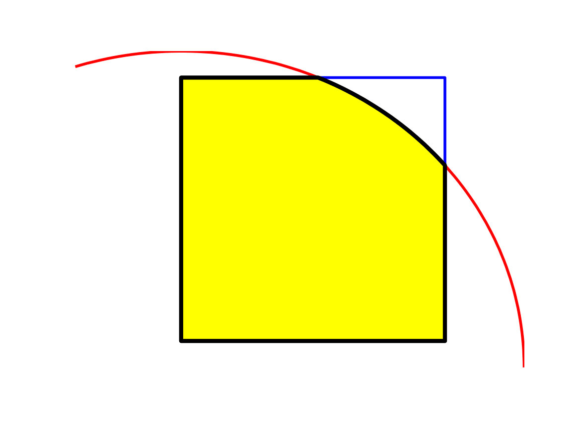
(a)	(b)	(c)

Figure 2: Three types of elements:(a)type A;(b)type B;(c)type C.

Therefore, trimmed elements are divided into three types, as depicted in Fig. 2.

• Type A is the curved pentagon;

• Type B is the curved quadrilateral;

• Type C is the curved triangle;

where the curved edge is part of the trimming curve. For each type, they segment the trimmed element to triangular ones. The triangular elements are further subdivided to two cases, i.e. a(normal) triangle with straight edges and a triangle with two straight and one curved edge, see Fig. 3. Let us denote these triangles as $T$ and $\tilde{T}$ respectively. For the ’normal’ triangle $T$ the integration points for the linear triangle(triangular element) are chosen. If $T$ has a curved edge, a series of triangulation is performed on $T$ in order to map $T$ to a rectangle.

(a)type A	(b)type B

Figure 3: Segmentation of elements with type A and type B.

2.2.1 Imposition of essential boundary condition

In isogeometric analysis, essential boundary conditions can not be imposed as in FEM, because NURBS basis functions do not satisfy the Kronecker delta property. For homogeneous essential boundary conditions, the coefficients of basis functions corresponding to boundary are set to zero. The imposition of non-homogeneous essential boundary conditions require special techniques such as modification of the weak form or the solution of an interpolation problem at the boundary; see e.g. [17].

In trimmed isogeometric analysis, additional challenges occur for imposing essential boundary condition. The boundary conditions need to be imposed on the trimming curves but the degree of freedom(DOF) is defined on the NURBS surface. Furthermore there is no mathematical relationship between these two representations. In [13], they use Lagrange multiplier method to impose essential boundary conditions on trimming curves. And we use the same method which is described in Section 4.

3 Improved isogeometric analysis on trimmed geometry

In this paper, we propose an improved method for IGA on trimmed geometries, by which improves the efficiency and accuracy of trimmed IGA.

The main contribution of our method is to modify the integration rules for the trimmed elements. For type C in  [13], a similar method is applied to generate integral points on the curved triangle, but for type B [13], a mapping from a rectangle to the curved quadrilateral element is used which avoids the triangular decomposition of the curved quadrilateral element. For type A, a decomposition is adopted but it is different from the method in  [13]. The curved pentagon is segmented to two quadrilaterals, one with a curved edge and the other is rectangular. Fig. 4 shows the decomposition of type A in our method.

The segmentation of trimmed elements of type A can be chosen on the basis of the intersection points. Suppose $P_{a}$ and $P_{b}$ are two intersection points, where $P_{b}$ is closer to the corner point which is trimmed out, then the trimmed element is segmented at point $P_{a}$.

Figure 4: The trimmed element of type A is decomposed to two quadrilaterals.

Except trimmed elements of type C, all trimmed elements are represented as quadrilaterals. For the curved quadrilateral which contains one curved edge as part of trimming curves, the mapping from unit rectangle is constructed as follows: according to the location of the curved edge, there are four types of curved quadrilaterals as shown in Fig. 5. Suppose $u_{2}>u_{1}$, where $u_{1},u_{2}$ are parameters of the trimming curve at the intersections. For each case, the mapping $Q$ between the curved quadrilateral and rectangle can be described as follows.

(a)	(b)
(c)	(d)

Figure 5: Trimmed element of type B.

(a): if $u_{1}$ is the parameter of the left intersection point, the mapping $Q$ is constructed as

$$\begin{split}X&=\phi_{X}\zeta+\frac{u-u_{1}}{u_{2}-u_{1}}(1-\zeta)\\ Y&=\phi_{Y}\zeta\end{split}$$ (1)

otherwise,

$$\begin{split}X&=\phi_{X}\zeta+\frac{u_{2}-u}{u_{2}-u_{1}}(1-\zeta)\\ Y&=\phi_{Y}\zeta\end{split}$$ (1^′)

(b): if $u_{1}$ is the parameter of the right intersection point, the mapping $Q$ is constructed as

$$\begin{split}X&=\phi_{X}(1-\zeta)+\frac{u-u_{1}}{u_{2}-u_{1}}\zeta\\ Y&=\phi_{Y}(1-\zeta)+\zeta\end{split}$$ (2)

otherwise,

$$\begin{split}X&=\phi_{X}(1-\zeta)+\frac{u_{2}-u}{u_{2}-u_{1}}\zeta\\ Y&=\phi_{Y}(1-\zeta)+\zeta\end{split}$$ (2^′)

(c): if $u_{1}$ is the parameter of the bottom intersection point, the mapping $Q$ is constructed as

$$\begin{split}X&=\phi_{X}\zeta\\ Y&=\phi_{Y}\zeta+\frac{u-u_{1}}{u_{2}-u_{1}}(1-\zeta)\end{split}$$ (3)

otherwise,

$$\begin{split}X&=\phi_{X}\zeta\\ Y&=\phi_{Y}\zeta+\frac{u_{2}-u}{u_{2}-u_{1}}(1-\zeta)\end{split}$$ (3^′)

(d): if $u_{1}$ is the parameter of the top intersection point, the mapping $Q$ is constructed as

$$\begin{split}X&=\phi_{X}(1-\zeta)+\zeta\\ Y&=\phi_{Y}(1-\zeta)+\frac{u-u_{1}}{u_{2}-u_{1}}\zeta\end{split}$$ (4)

otherwise,

$$\begin{split}X&=\phi_{X}(1-\zeta)+\zeta\\ Y&=\phi_{Y}(1-\zeta)+\frac{u_{2}-u}{u_{2}-u_{1}}\zeta\end{split}$$ (4^′)

Guass quadrature is commonly used in isogeometric FE approaches. Compared to the method proposed by Kim et al. [13], the proposed method leads to less integration points. Fig. 6 shows the distribution of Gauss points in our approach compared to the approach in [13] for one trimmed element. In fact, the reduction of integral points can be estimated. Suppose $n$ Gauss points are chosen for the normal triangle, and $m$ Gauss points are chosen for the curved triangle. As the number of integral points for quadrilateral element is the same with curved triangle, we can give the number of integral points for each type of trimmed element, see Table. 1.

Table 1: Comparison of the number of integral points.

element	original method	our method
type A	2n+m	2m
type B	n+m	m
type C	m	m

(a)	(b)
(c)	(d)

Figure 6: Integration points and segmentation of trimmed elements.(a)(c) type A and type B elements in  [13], (b)(d) type A and type B elements in our method.

4 Numerical examples

In this section, we solve the Poisson equation on several trimmed geometries to show the effectiveness of our method, and compare our results with results obtained by the method in [13].

The Poisson equation with Dirichlet boundary condition is given by,

$$\left\{\begin{aligned} -\Delta u&=f\\ u|_{\partial\Omega}&=g,\end{aligned}\right.$$ (5)

where $\Omega$ is the trimmed geometry represented by a NURBS surface and several trimming NURBS curves.

We use Lagrange multiplier method to impose the essential boundary condition as [13] does. The Lagrange multipliers $\bm{\lambda}(u)$ are supposed to be expressed as

$$\bm{\lambda}(u)=\sum_{i=1}^{l}R_{i}^{c}(u)\lambda_{i}$$

where $R_{i}^{c}(u)$ is the NURBS basis function of trimming curve. The weak form with Lagrange multipliers is discretized as equations

$$\bm{K}\bm{U}+\bm{A^{T}}\bm{\lambda} =\bm{f}$$

$$\bm{A}\bm{U} =\bm{b}$$

where

$$K_{ij}=\int_{\Omega}R_{i}^{s}R_{j}^{s}d\Omega,\quad f_{i}=\int_{\Omega}R_{i}^{s}fd\Omega$$

$$A_{ij}=\int_{\partial\Omega}R_{i}^{c}R_{j}^{s}d\partial\Omega,\quad b_{i}=\int_{\partial\Omega}R_{i}^{c}gd\partial\Omega$$

the $R_{i}^{c}(u)$ also denotes the NURBS basis function of trimming curve, $R_{i}^{s}(s,t)$ denotes the NURBS basis function of spline surface. $\bigcup\Omega_{i}=\Omega,\Xi=\{\Omega_{i}\}_{i}$. For subregion $\Omega_{i}$, we can use Gaussian points to compute the integration. More details can be found in [13].

For the method in  [13], basis functions are NURBS basis functions. Three Gaussian points are used in each direction for quadrilateral element, and seven Gaussian points are used for the regular triangle.

(a)	(b)	(c)

Figure 7: Integration points and segmentation of trimmed elements with $3\times 3$ elements: (a) computational domain of EX1;(b) integration points in  [13];(c) integration points in the proposed method.

In the first example, we choose a very simple geometry, the computational domain is fan-shaped. It is constructed by trimming a corner of a rectangle using an arc represented by a NURBS curve. In this example, we compare the corresponding $L^{2}$ error of numerical solution, and the condition number of stiffness matrix with the method in  [13] as shown in Table 2. The error plot is shown in Fig. 8 which is more illustrative. We also compare the computational cost of Ex1 as presented in Table 3, where $T_{e}$ represents the trimmed element and $\tilde{T_{e}}$ represents the integration element after the decomposition of $T_{e}$.

Table 2: Comparison of our method with the proposed method in  [13] for Ex1.

	Method in  [13]		Our method
Number of element	Cond.	$L^{2}$ error	Cond.	$L^{2}$ error
$5\times 5$	$7.5051\times 10^{4}$	0.0209621	$5.0469\times 10^{4}$	0.0190196
$10\times 10$	$2.2417\times 10^{10}$	0.0145103	$1.5930\times 10^{10}$	0.00969233
$20\times 20$	$4.3386\times 10^{9}$	0.0096861	$2.9344\times 10^{9}$	0.00487051

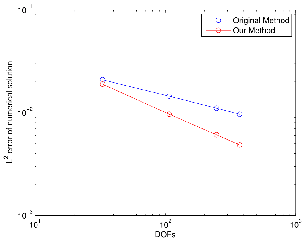
Figure 8: Comparison of $L^{2}$ error.

We use the method presented in [12] to find all the active elements, and construct the mapping from the unit square $[0,1]\times[0,1]$ to each trimmed element as described in section 3. When the spline surface consists of $3\times 3$ elements, with our method, the distribution of the integration points on the computational domain is more regular than the method in  [13] as illustrated in Fig. 7. The corresponding numerical solution is shown in Fig. 9. From Table 2, we can see that the condition number of the stiffness matrix and the $L^{2}$ error of the numerical solution is reduced almost by one half compared to the method in  [13] on the refined grid.

(a)	(b)	(c)

Figure 9: Comparison of numerical solution with $20\times 20$ grid.(a) the method in  [13];(b) our method;(c)exact solution.

(a)	(b)

(c)	(d)

Figure 10: The computational domain of EX2. (a) elements and integral points of the method in  [13];(b)enlarge the area of yellow rectangle in (a);(c) elements and integral points of our method;(d)enlarge the area of yellow rectangle in (c).

(a)	(b)

(c)	(d)

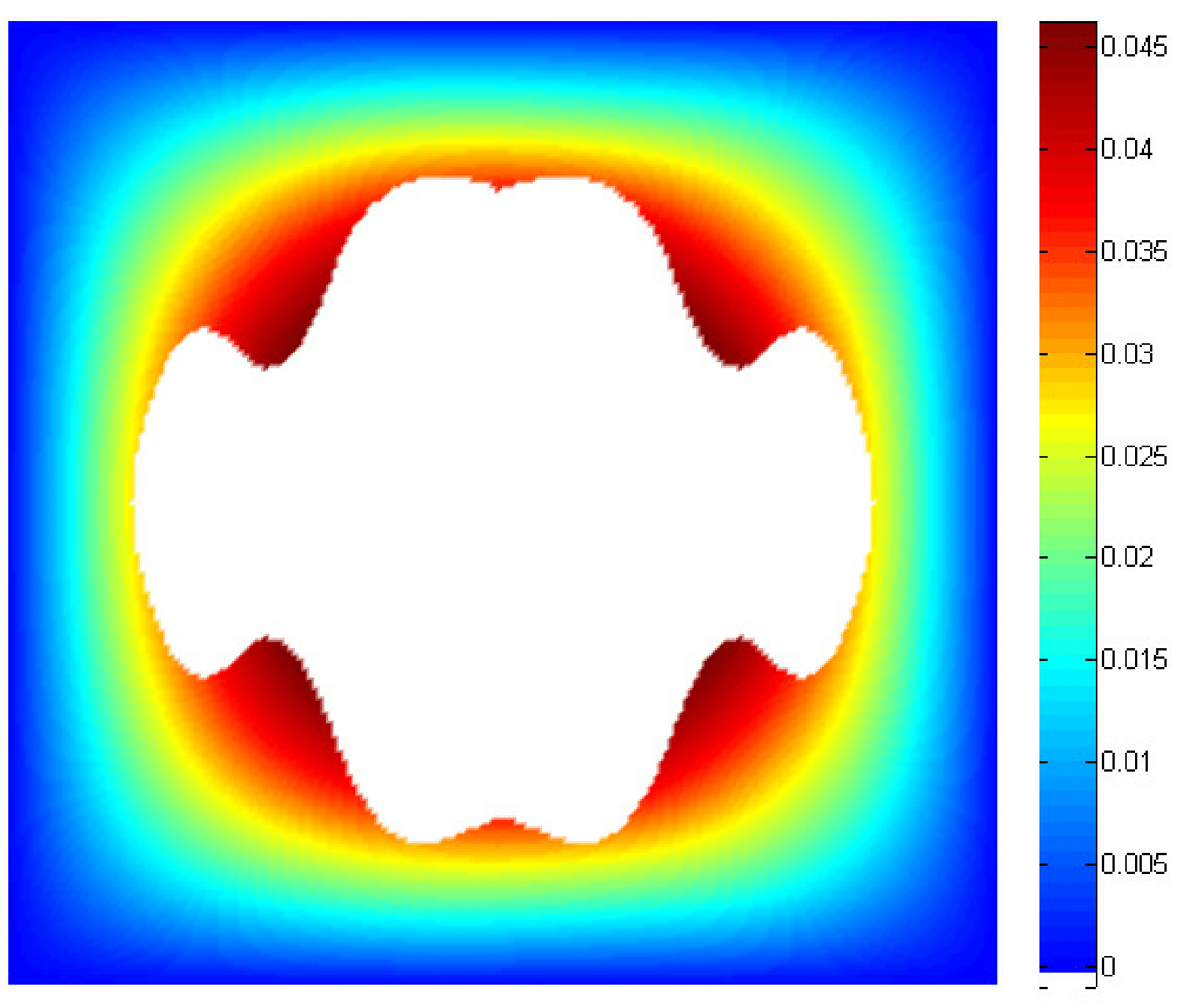
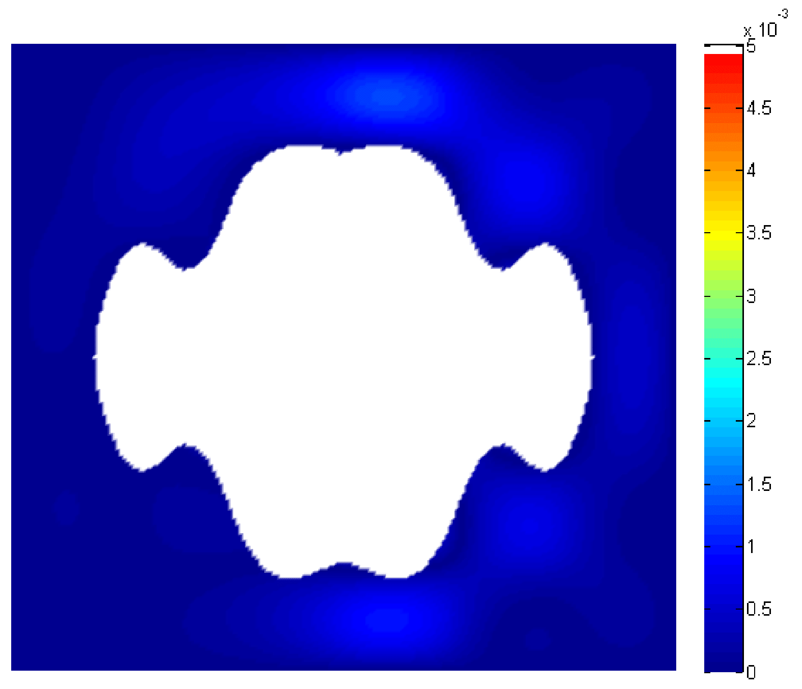
(e)	(f)

Figure 11: The computational domain of EX3: (a) elements and integral points of the method in  [13];(b)enlarge the area of yellow rectangle in (a);(c) elements and integral points of our method;(d) enlarge the area of yellow rectangle in (c);(e)numerical solution;(f)$L^{2}$ error is $4.43065\times 10^{-4}$.

In the second example, we construct a computational domain with complex geometry, where the rectangle is trimmed by a closed spline curve. There are two protrusions in the interior of the final trimmed geometry. In this example, the surface contains $6\times 6$ elements first. However, there are other kind of trimmed elements except of three types we processed in this coarse mesh, so local refinement is performed on the surface as described in [12] until there are only three types of trimmed elements. In this example, there are many type B trimmed elements, as shown in Fig. 12 . The element of type B is decomposed into two triangles with the method in  [13], integration on this element then becomes integration on these two triangles. In the proposed method, we construct a mapping from type B element to rectangle directly while keeping the number of integral elements. Our method can reduce a half integral points and integral elements for this type of trimmed element. For type A, one third of integral points and integral elements can be reduced by our method.

In the third example, the number of trimmed elements of type A and type C are more than type B, in this case the reduction of integral points and integral elements is not as significant as the first example. It can be clearly observed from Table 2.

A round hole is trimmed out from a rectangle as computational domain in the last example. In this example, the number of trimmed elements of type A becomes more and more during mesh refinement process , and the reduction of integral elements is clearly demonstrated.

(a)	(b)

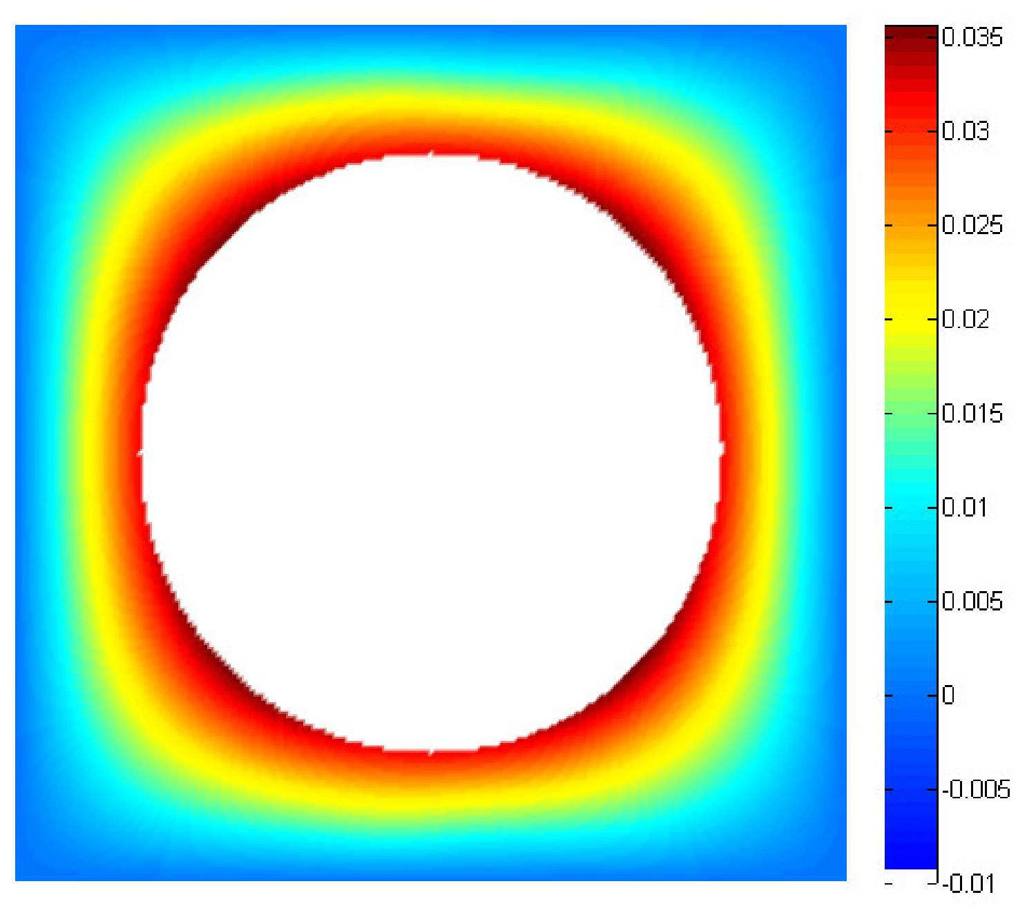
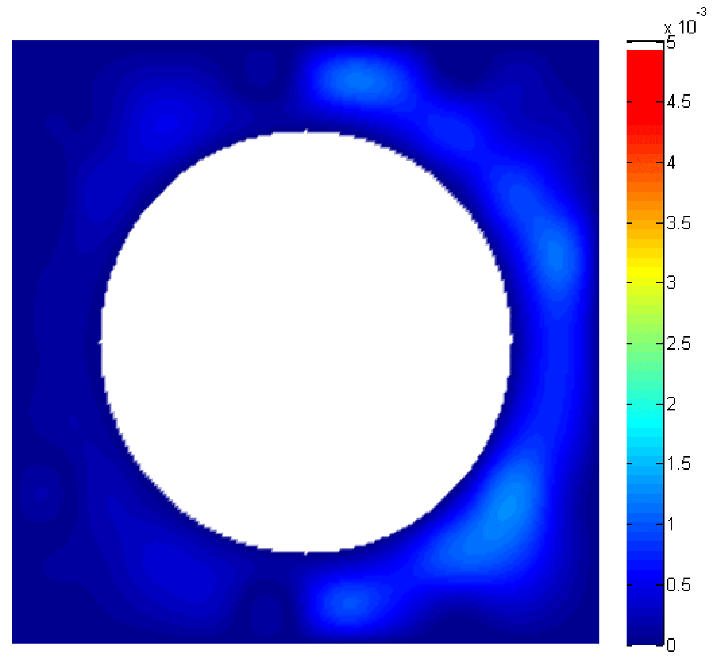
(c)	(d)

Figure 12: The computational domain of EX4. (a)elements and integral points of the method in  [13];(b)elements and integral points of our method; (c)numerical solution of $10\times 10$ grid;(d)$L^{2}$ error is $3.26665\times 10^{-4}$.

Table 3: Comparison of computational cost with the Method in  [13]

	Mesh Size	Number of $T_{e}$	Number of $\tilde{T}_{e}$		Number of integral points in $T_{e}$
			Method in  [13]	Our method	Method in  [13]	Our method
Ex1	$3\times 3$	5	9	5	73	45
	$10\times 10$	17	31	19	251	171
	$20\times 20$	37	71	45	571	405
Ex2	$6\times 6$	47	98	60	780	486
Ex3	$6\times 6$	48	100	72	796	648
Ex4	$3\times 3$	8	20	12	156	108
	$10\times 10$	28	60	40	476	360
	$20\times 20$	56	112	76	896	684

5 Conclusion

In this paper, we propose an improved method of isogeometric analysis over trimmed geometries on two-dimensional planar computational domain. By the proposed method, the integral elements and integral points in analysis process can be reduced significantly, which improves the efficiency of analysis. Moreover, compared with the previous method, the distribution of integral points is more regular, and the accuracy of numerical solution is also improved. Extension to three-dimensional isogeometric analysis  [24, 25] will be a part of future work.

References

References

- [1] Michael Breitenberger, Kai-Uwe Bletzinger, Roland Wüchner. Isogeometric layout optimization of shell structures using trimmed NURBS surfaces. 10th World Congress on Structural and Multidisciplinary Optimization, May 19-24, 2013, Orlando, Florida, USA.
- [2] M. Brovka, J.I. López, J.M. Escobar, J.M. Cascón, R.Montenegro. A new method for T-spline parameterization of complex 2D geometries. Engineering with Computers, 2014, 30:457-473.
- [3] G. Beer, B. Marussig, J. Zechner, et al. Boundary Element Analysis with trimmed NURBS and a generalized IGA approach. Eprint Arxiv, 2014(1):282-91.
- [4] M. Breitenberger, A. Apostolatos, B. Philipp, et al. Analysis in computer aided design: Nonlinear isogeometric B-Rep analysis of shell structures. Computer Methods in Applied Mechanics & Engineering, 2015, 284:401-457.
- [5] J.A. Cottrell, T.J.R. Hughes, Y. Bazilevs. Isogeometric analysis: Toward integration of CAD and FEA. Wiley; 2009.
- [6] E. Cohen, T. Martin, R.M. Kirby, T. Lyche, R.F. Riesenfeld. Analysis-aware modeling: Understanding quality considerations in modeling for isogeometric analysis. Comput. Methods Appl. Mech. Engrg., 2010, 199:334-356.
- [7] Chiu Ling Chan, Cosmin Anitescu, Timon Rabczuk. Volumetric parametrization from a level set boundary representation with PHT-splines. Computer-Aided Design, 2017, 82: 29-41.
- [8] J.S. Deng, F.L. Chen, X. Li, C.Q. Hu, W.H. Tong, Z.W. Yang, Y.Y. Feng. Polynomial splines over hierarchical T-meshes. Graphical Models, 2008, 70:76-86.
- [9] Antonella Falini, Jaka Speh, Bert Juttler. Planar domain parameterization with THB-splines. Computer Aided Geometric Design, 2015, 35-36: 95-108.
- [10] T.J.R. Hughes, J.A. Cottrell, Y. Bazilevs. Isogeometric analysis: CAD, finite elements, NURBS, exact geometry and mesh refinement. Comput. Methods Appl. Mech. Engrg. 2005,194: 4135-4195.
- [11] Kjetil Andr Johannessen, Trond Kvamsdal, Tor Dokken. Isogeometric analysis using LR B-splines. Comput. Methods Appl. Mech. Engrg., 2014, 269: 471-514.
- [12] Hyun-Jung Kim, Yu-Deok Seo, Sung-Kie Youn. Isogeometric analysis for trimmed CAD surfaces. Comput. Methods Appl. Mech. Engrg., 2009, 198:2982-2995.
- [13] Hyun-Jung Kim, Yu-Deok Seo, Sung-Kie Youn. Isogeometric analysis with trimming technique for problems of arbitrary complex topology. Comput. Methods Appl. Mech. Engrg., 2010,199:2796-2812.
- [14] P. Kang, S.K. Youn. Isogeometric shape optimization of trimmed shell structures. Structural & Multidisciplinary Optimization, 2015, 53(4):825-845.
- [15] B. Marussig, J. Zechner, G. Beer, et al. Stable isogeometric analysis of trimmed geometries. Computer Methods in Applied Mechanics & Engineering, 2016, 316:497-521.
- [16] Benjamin Marussig, Thomas J. R. Hughes. A Review of Trimming in Isogeometric Analysis: Challenges, Data Exchange and Simulation Aspects. Archives of Computational Methods in Engineering, 2017, doi:10.1007/s11831-017-9220-9.
- [17] M. Ruess, D. Schillinger, A.I. Özcan, et al. Weak coupling for isogeometric analysis of non-matching and trimmed multi-patch geometries. Computer Methods in Applied Mechanics & Engineering, 2014, 269(2):46-71.
- [18] T.W. Sederberg, J. Zheng, A. Bakenov, A. Nasri. T-Splines and T-NURCCs. ACM Trans. Graph., 2003, 22:477-484.
- [19] J. Shen, J. Kosinka, M.A. Sabin, et al. Conversion of trimmed NURBS surfaces to Catmull-Clark subdivision surfaces. Computer Aided Geometric Design, 2014, 31:486-498.
- [20] Robert Schmidt, Roland Wuchner, Kai-Uwe Bletzinger. Isogeometric analysis of trimmed NURBS geometries. Comput. Methods Appl. Mech. Engrg., 2012, 241-244:93-111.
- [21] Yingjun Wang, David J. Benson, Attila P. Nagy. A multi-patch nonsingular isogeometric boundary element method using trimmed elements. Computational Mechanics, 2015, 56(1):173-191.
- [22] G. Xu, B. Mourrain, R. Duvigneau, A. Galligo. Optimal analysis-aware parameterization of computational domain in 3D isogeometric analysis. Computer-Aided Design, 2013, 45:812-821.
- [23] G. Xu, B. Mourrain, R. Duvigneau, A. Galligo. Parameterization of computational domain in isogeometric analysis: methods and comparison. Computer Methods in Applied Mechanics and Engineering 200(2011) 2021-2031.
- [24] G. Xu, T. H. Kwok, and C. C. Wang. Isogeometric computation reuse method for complex objects with topology-consistent volumetric parameterization. Computer-Aided Design 91(2017) 1-13.
- [25] G. Xu, B. Mourrain, R. Duvigneau, A. Galligo. Analysis-suitable volume parameterization of multi-block computational domain in isogeometric applications. Computer-Aided Design 45(2013) 395-404.
- [26] J. Xu, F. Chen, J. Deng. Two-dimensional domain decomposition based on skeleton computation for parameterization and isogeometric analysis. Computer Methods in Applied Mechanics and Engineering 284(2015) 541-555
- [27] Xuefeng Zhu, Ping Hu, Zheng-Dong Ma. B++ splines with applications to isogeometric analysis. Comput. Methods Appl. Mech. Engrg., 2016, 311:503-536.
- [28] Xuefeng Zhu, Zheng-Dong Ma, Ping Hu. Nonconforming isogeometric analysis for trimmed CAD geometries using FETI method. https://www.researchgate.net/publication/307545322.