A Channel-Based Perspective on Conjugate Priors

Abstract

A desired closure property in Bayesian probability is that an updated posterior distribution be in the same class of distributions — say Gaussians — as the prior distribution. When the updating takes place via a statistical model, one calls the class of prior distributions the ‘conjugate priors’ of the model. This paper gives (1) an abstract formulation of this notion of conjugate prior, using channels, in a graphical language, (2) a simple abstract proof that such conjugate priors yield Bayesian inversions, and (3) a logical description of conjugate priors that highlights the required closure of the priors under updating. The theory is illustrated with several standard examples, also covering multiple updating.

1 Introduction

The main result of this paper, Theorem 6.3, is mathematically trivial. But it is not entirely trivial to see that this result is trivial. The effort and contribution of this paper lies in setting up a framework — using the abstract language of channels, Kleisli maps, and string diagrams for probability theory — to define the notion of conjugate prior in such a way that there is a trivial proof of the main statement, saying that conjugate priors yield Bayesian inversions. This is indeed what conjugate priors are meant to be.

Conjugate priors form a fundamental topic in Bayesian theory. They are commonly described via a closure property of a class of prior distributions, namely as being closed under certain Bayesian updates. Conjugate priors are especially useful because they do not only involve a closure property, but also a particular structure, namely an explicit function that performs an analytical computation of posterior distributions via updates of the parameters. This greatly simplify Bayesian analysis. For instance, the $\mathrm{Beta}$ distribution is conjugate prior to the Bernoulli (or ‘flip’) distribution, and also to the binomial distribution: updating a $\mathrm{Beta}(\alpha,\beta)$ prior via a Bernoulli/binomial statistical model yields a new $\mathrm{Beta}(\alpha^{\prime},\beta^{\prime})$ prior, with adapted parameters $\alpha^{\prime},\beta^{\prime}$ that can be computed explicitly from $\alpha,\beta$ and the observation at hand. Despite this importance, the descriptions in the literature of what it means to be a conjugate prior are remarkably informal. One does find several lists of classes of distributions, for instance at Wikipedia, together with formulas about how to re-compute parameters. The topic has a long and rich history in statistics (see e.g. [Bishop, 2006]), with much emphasis on exponential families [Diaconis and Ylvisaker, 1979], but a precise, general definition is hard to find.

We briefly review some common approaches, without any pretension to be complete: the definition in [Alpaydin, 2010] is rather short, based on an example, and just says: “We see that the posterior has the same form as the prior and we call such a prior a conjugate prior.” Also [Russell and Norvig, 2003] mentions the term ‘conjugate prior’ only in relation to an example. There is a separate section in [Bishop, 2006] about conjugate priors, but no precise definition. Instead, there is the informal description “…the posterior distribution has the same functional form as the prior.” The most precise definition (known to the author) is in [Bernardo and Smith, 2000, §5.2], where the conjugate family with respect to a statistical model, assuming a ‘sufficient statistic’, is described. It comes close to our channel-based description, since it explicitly mentions the conjugate family as a conditional probability distribution with (re-computed) parameters. The approach is rather concrete however, and the high level of mathematical abstraction that we seek here is missing in [Bernardo and Smith, 2000].

This paper presents a novel systematic perspective for precisely defining what conjugate priorship means, both via diagrams and via (probabilistic) logic. It uses the notion of ‘channel’ as starting point. The basis of this approach lies in category theory, especially effectus theory [Jacobs, 2015, Cho et al., 2015]. However, we try to make this paper accessible to non category theorists, by using the term ‘channel’ instead of morphism in a Kleisli category of a suitable monad. Moreover, a graphical language is used for channels that hopefully makes the approach more intuitive. Thus, the emphasis of the paper is on what it means to have conjugate priors. It does not offer new perspectives on how to find/obtain them.

The paper is organised as follows. It starts in Section 2 with a high-level description of the main ideas, without going into technical details. Preparatory definitions are provided in Sections 3 and 4, dealing with channels in probabilistic computation, with a diagrammatic language for channels, and with Bayesian inversion. Then, Section 5 contains the novel channel-based definition of conjugate priorship; it also illustrates how several standard examples fit in this new setting. Section 6 establishes the (expected) close relationship between conjugate priors and Bayesian inversions. Section 7 then takes a fresh perspective, by re-describing the Bayesian-inversion based formulation in more logical terms, using validity and updating. This re-formulation captures the intended closure of a class of priors under updating in the most direct manner. It is used in Section 8 to illustrate how multiple updates are handled, typically via a ‘sufficient statistic’.

2 Main ideas

This section gives an informal description of the main ideas underlying this paper. It starts with a standard example, and then proceeds with a step-by-step introduction to the essentials of the perspective of this paper.

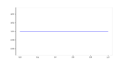
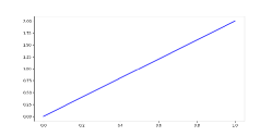
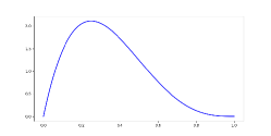
Figure 1: Uniform prior, and two posterior probability density functions on $[0,1]$, after observing head, and after observing head-tail-tail-tail. These functions correspond respectively to $\mathrm{Beta}(1,1)$, $\mathrm{Beta}(2,1)$, $\mathrm{Beta}(2,4)$. Example 4.2 below explains how these three plots are obtained, via actual Bayesian updates (inversions), and not by simply using the $\mathrm{Beta}$ functions.

A well-known example in Bayesian reasoning is inferring the (unknown) bias of a coin from a sequence of consecutive head/tail observations. The bias is a number $r\in[0,1]$ in the unit interval, giving the ‘Bernoulli’ or ‘flip’ probability $r$ for head, and $1-r$ for tail. Initially we assume a uniform distribution for $r$, as described by the constant probability density function (pdf) on the left in Figure 1. After observing one head, this pdf changes to the second picture. After observing head-tail-tail-tail we get the third pdf. These pictures are obtained by Bayesian inversion, see Section 4.

It is a well-known fact that all the resulting distributions are instances of the $\mathrm{Beta}(\alpha,\beta)$ family of distributions, for different parameters $\alpha,\beta$. After each observation, one can re-compute the entire updated distribution, via Bayesian inversion, as in Example 4.2. But in fact there is a much more efficient way to obtain the revised distribution, namely by computing the new parameter values: increment $\alpha$ by one, for head, and increment $\beta$ by one for tail, see Examples 5.3 and 7.3 for details. The family of distributions $\mathrm{Beta}(\alpha,\beta)$, indexed by parameters $\alpha,\beta$, is thus suitably closed under updates with Bernoulli. It is the essence of the statement that $\mathrm{Beta}$ is conjugate prior to Bernoulli. This will be made precise later on.

Let $X=(X,\Sigma)$ be a measurable space, where $\Sigma\subseteq\mathcal{P}(X)$ is a $\sigma$-algebra of measurable subsets. We shall write $\mathcal{G}(X)$ for the set of probability distributions on $X$. Elements $\omega\in\mathcal{G}(X)$ are thus countably additive functions $\omega\colon\Sigma\rightarrow[0,1]$ with $\omega(X)=1$.

Idea 1:

A family of distributions on $X$, indexed by a measurable space $P$ of parameters, is a (measurable) function $P\rightarrow\mathcal{G}(X)$. Categorically, such a function is a Kleisli map for $\mathcal{G}$, considered as monad on the category of measurable spaces (see Section 3). These Kleisli maps are also called channels, and will be written simply as arrows $P\rightarrow X$, or diagrammatically as boxes   where we imagine that information is flowing upwards.

The study of families of distributions goes back a long way, e.g. as ‘experiments’ [Blackwell, 1951].

Along these lines we shall describe the family of $\mathrm{Beta}$ distributions as a channel with $P=\mathbb{R}_{>0}\times\mathbb{R}_{>0}$ and $X=[0,1]$, namely as function:

(1)

For $(\alpha,\beta)\in\mathbb{R}_{>0}\times\mathbb{R}_{>0}$ there is the probability distribution $\mathrm{Beta}(\alpha,\beta)\in\mathcal{G}([0,1])$ determined by its value on a measurable subset $M\subseteq[0,1]$, which is obtained via integration:

$$\begin{array}[]{rcl}\mathrm{Beta}(\alpha,\beta)(M)&=&{\displaystyle\int_{M}}\frac{x^{\alpha-1}(1-x)^{\beta-1}}{B(\alpha,\beta)}{\kern 1.99997pt}\mathrm{d}{\kern 0.29999pt}x,\end{array}$$ (2)

where $B(\alpha,\beta)=\int_{[0,1]}x^{\alpha-1}(1-x)^{\beta-1}{\kern 1.99997pt}\mathrm{d}{\kern 0.29999pt}x$ is a normalisation constant.

A conjugate prior relationship involves a family of distributions $P\rightarrow\mathcal{G}(X)$ which is closed wrt. updates based on observations (or: data) from a separate domain $O$. Each ‘parameter’ element $x\in X$ gives rise to a separate distribution on $O$. This is what is usually called a statistical or parametric model. We shall also describe it as a channel.

Idea 2:

The observations for a family $P\rightarrow\mathcal{G}(X)$ arise via another “Kleisli” map $X\rightarrow\mathcal{G}(O)$ representing the statistical model. Conjugate priorship will be defined for two such composable channels $P\rightarrow X\rightarrow O$, where $O$ is the space of observations.

In the above coin example, the space $O$ of observations is the two-element set $2=\{0,1\}$ where $0$ is for tail and $1$ for head. The Bernoulli channel is written as $\mathrm{Flip}\colon[0,1]\rightarrow\mathcal{G}(2)$. A probability $r\in[0,1]$ determines a Bernoulli/flip/coin probability distribution $\mathrm{Flip}(r)\in\mathcal{G}(2)$ on $2$, formally sending the subset $\{1\}$ to $r$ and $\{0\}$ to $1-r$.

Idea 3:

A channel $c\colon P\rightarrow X$ is a conjugate prior to a channel $d\colon X\rightarrow O$ if there is a parameter translation function $h\colon P\times O\rightarrow P$ satisfying a suitable equation.

The idea is that $c(p)$ is a prior, for $p\in P$, which gets updated via the statistical model (channel) $d$, in the light of observation $y\in O$. The revised, updated distribution is $c(h(p,y))$. The model $d$ is usually written as a conditional probability $d(y\mid\theta)$.

In the coin example we have $h\colon\mathbb{R}_{>0}\times\mathbb{R}_{>0}\times 2\rightarrow\mathbb{R}_{>0}\times\mathbb{R}_{>0}$ given by $h(\alpha,\beta,1)=(\alpha+1,\beta)$ and $h(\alpha,\beta,0)=(\alpha,\beta+1)$, see Example 5.3 below for more information.

What has been left unexplained is the ‘suitable’ equation that the parameter translation function $h\colon P\times O\rightarrow P$ should satisfy. It is not entirely trivial, because it is an equation between channels in what is called the Kleisli category $\mathcal{K}{\kern-2.15277pt}\ell(\mathcal{G})$ of the Giry monad $\mathcal{G}$. At this stage we need to move to a more categorical description. The equation, which will appear in Definition 5.1, bears similarities with the notion of Bayesian inversion, which will be introduced in Section 4.

3 Channels and conditional probabilities

This section will describe conditional probabilities as arrows and will show how to compose them. Thereby we are entering the world of category theory. We aim to suppress the underlying categorical machinery and make this work accessible to readers without such background. For those with categorical background knowledge: we will be working in the Kleisli categories of the distribution monad $\mathcal{D}$ for discrete probability, and of the Giry monad $\mathcal{G}$ for continuous probability, see e.g. [Giry, 1982, Panangaden, 2009, Jacobs, 2017]. Discrete distributions may be seen as a special case of continuous distributions, via a suitable inclusion map $\mathcal{D}\rightarrow\mathcal{G}$. Hence one could give one account, using $\mathcal{G}$ only. However, in computer science, unlike for instance in statistics, discrete distributions are so often used that they merit separate treatment.

We thus start with discrete probability. We write a (finite, discrete) distribution on a set $X$ as a formal convex sum $r_{1}|{\kern 1.00006pt}x_{1}{\kern 1.00006pt}\rangle+\cdots+r_{n}|{\kern 1.00006pt}x_{n}{\kern 1.00006pt}\rangle$ of elements $x_{i}\in X$ and probabilities $r_{i}\in[0,1]$ with $\sum_{i}r_{i}=1$. The ‘ket’ notation $|{\kern 1.00006pt}-{\kern 1.00006pt}\rangle$ is syntactic sugar, used to distinguish elements of $x$ from their occurrence $|{\kern 1.00006pt}x{\kern 1.00006pt}\rangle$ in such formal convex sums. A distribution as above can be identified with a ‘probability mass’ function $\omega\colon X\rightarrow[0,1]$ which is $r_{i}$ on $x_{i}$ and $0$ elsewhere. We often implicitly identify distributions with such functions. We shall write $\mathcal{D}(X)$ for the set of distributions on $X$.

We shall focus on functions of the form $c\colon X\rightarrow\mathcal{D}(Y)$. They give, for each element $x\in X$ a distribution $c(x)$ on $Y$. Hence such functions form an $X$-indexed collection $\big{(}c(x)\big{)}_{x\in X}$ of distributions $c(x)$ on $Y$. They can be understood as conditional probabilities $P(y\mid x)=r$, if $c(x)$ is of the form $\cdots r|{\kern 1.00006pt}y{\kern 1.00006pt}\rangle\cdots$, with weight $r=c(x)(y)\in[0,1]$ for $y\in Y$. Thus, by construction, $\sum_{y}P(y\mid x)=1$, for each $x\in X$. Moreover, if the sets $X$ and $Y$ are finite, we can describe $c\colon X\rightarrow\mathcal{D}(Y)$ as a stochastic matrix, with entries $P(y\mid x)$, adding up to one — per row or column, depending on the chosen orientation of the matrix.

We shall often write functions $X\rightarrow\mathcal{D}(Y)$ simply as arrows $X\rightarrow Y$, call them ‘channels’, and write them as ‘boxes’ in diagrams. This arrow notation is justified, because there is a natural way to compose channels, as we shall see shortly. But first we describe state transformation, also called prediction. Given a channel $c\colon X\rightarrow\mathcal{D}(Y)$ and a state $\omega\in\mathcal{D}(X)$, we can form a new state, written as $c\gg\omega$, on $Y$. It is defined as:

$$\begin{array}[]{rcl}c\gg\omega&\coloneqq&{\displaystyle\sum_{y}}\big{(}\sum_{x}\omega(x)\cdot c(x)(y)\big{)}\big{|}y\big{\rangle}.\end{array}$$ (3)

The outer sum $\sum_{y}$ is a formal convex sum, whereas the inner sum $\sum_{x}$ is an actual sum in the unit interval $[0,1]$. Using state transformation $\gg$ it is easy to define composition of channels: given functions $c\colon X\rightarrow\mathcal{D}(Y)$ and $d\colon Y\rightarrow\mathcal{D}(Z)$, we use the ordinary composition symbol $\mathrel{\circ}$ to form a composite channel $d\mathrel{\circ}c\colon X\rightarrow\mathcal{D}(Z)$, where:

$$\begin{array}[]{rcccl}(d\mathrel{\circ}c)(x)&\coloneqq&d\gg c(x)&=&{\displaystyle\sum_{z\in Z}}\big{(}\sum_{y}c(x)(y)\cdot d(y)(z)\big{)}\big{|}z\big{\rangle}.\end{array}$$ (4)

Essentially, this is matrix composition for stochastic matrices. Channel composition $\mathrel{\circ}$ is associative, and also has a neutral element, namely the identity channel $\eta\colon X\rightarrow X$ given by the ‘Dirac’ function $\eta(x)=1|{\kern 1.00006pt}x{\kern 1.00006pt}\rangle$. It is not hard to see that $(d\mathrel{\circ}c)\gg\omega=d\gg(c\gg\omega)$.

We turn to channels in continuous probability. As already mentioned in Section 2, we write $\mathcal{G}(X)$ for the set of probability distributions $\omega\colon\Sigma_{X}\rightarrow[0,1]$, where $X=(X,\Sigma_{X})$ is a measurable space. These probability distributions are (also) called states. The set $\mathcal{G}(X)$ carries a $\sigma$-algebra itself, but that does not play an important role here. Each element $x\in X$ yields a probability measure $\eta(x)\in\mathcal{G}(X)$, with $\eta(x)(M)=\mathbf{1}_{M}(x)$, which is $1$ if $x\in M$ and $0$ otherwise. This map $\mathbf{1}_{M}\colon X\rightarrow[0,1]$ is called the indicator function for the subset $M\in\Sigma_{X}$.

For a state/measure $\omega\in\mathcal{G}(X)$ and a measurable function $f\colon X\rightarrow\mathbb{R}_{\geq 0}$ we write $\int f{\kern 1.99997pt}\mathrm{d}{\kern 0.29999pt}\omega$ for the Lebesgue integral, if it exists. We follow the notation of [Jacobs, 2013] and refer there for details, or alternatively, to [Panangaden, 2009]. We recall that an integral $\int_{M}f{\kern 1.99997pt}\mathrm{d}{\kern 0.29999pt}\omega$ over a measurable subset $M\subseteq X$ of the domain of $f$ is defined as $\int\mathbf{1}_{M}\cdot f{\kern 1.99997pt}\mathrm{d}{\kern 0.29999pt}\omega$, and that $\int\mathbf{1}_{M}{\kern 1.99997pt}\mathrm{d}{\kern 0.29999pt}\omega=\omega(M)$. Moreover, $\int f{\kern 1.99997pt}\mathrm{d}{\kern 0.29999pt}\eta(x)=f(x)$.

For a measurable function $g\colon X\rightarrow Y$ between measurable spaces $X,Y$ there is the ‘push forward’ function $\mathcal{G}(g)\colon\mathcal{G}(X)\rightarrow\mathcal{G}(Y)$, given by $\mathcal{G}(g)(\omega)(N)=\omega\big{(}g^{-1}(N)\big{)}$. It satisfies:

$$\begin{array}[]{rcl}\displaystyle\int f{\kern 1.99997pt}\mathrm{d}{\kern 0.29999pt}\mathcal{G}(g)(\omega)&=&\int f\mathrel{\circ}g{\kern 1.99997pt}\mathrm{d}{\kern 0.29999pt}\omega.\end{array}$$ (5)

Often, the measurable space $X$ is a subset $X\subseteq\mathbb{R}$ of the real numbers and a probability distribution $\omega$ on $X$ is given by a probability density function (pdf), that is, by a measurable function $f\colon X\rightarrow\mathbb{R}_{\geq 0}$ with $\int_{X}f(x){\kern 1.99997pt}\mathrm{d}{\kern 0.29999pt}x=1$. Such a pdf $f$ gives rise to a state $\omega\in\mathcal{G}(X)$, namely:

$$\begin{array}[]{rcl}\omega(M)&=&\displaystyle\int_{M}f(x){\kern 1.99997pt}\mathrm{d}{\kern 0.29999pt}x.\end{array}$$ (6)

We then write $\omega=\int f$.

In this continuous context a channel is a measurable function $c\colon X\rightarrow\mathcal{G}(Y)$, for measurable spaces $X,Y$. Like in the discrete case, it gives an $X$-indexed collection $(\big{(}c(x)\big{)}_{x\in X}$ of probability distributions on $Y$. The channel $c$ can transform a state $\omega\in\mathcal{G}(X)$ on $X$ into a state $c\gg\omega\in\mathcal{G}(Y)$ on $Y$, given on a measurable subset $N\subseteq Y$ as:

$$\begin{array}[]{rcl}\big{(}c\gg\omega\big{)}(N)&=&\displaystyle\int c(-)(N){\kern 1.99997pt}\mathrm{d}{\kern 0.29999pt}\omega.\end{array}$$ (7)

For another channel $d\colon Y\rightarrow\mathcal{G}(Z)$ there is a composite channel $d\mathrel{\circ}c\colon X\rightarrow\mathcal{G}(Z)$, via integration:

$$\begin{array}[]{rcccl}\big{(}d\mathrel{\circ}c\big{)}(x)(K)&\coloneqq&\big{(}d\gg c(x)\big{)}(K)&=&\displaystyle\int d(-)(K){\kern 1.99997pt}\mathrm{d}{\kern 0.29999pt}c(x)\end{array}$$ (8)

In many situations a channel $c\colon X\rightarrow\mathcal{G}(Y)$ is given by an indexed probability density function (pdf) $u\colon X\times Y\rightarrow\mathbb{R}_{\geq 0}$, with $\int u(x,y){\kern 1.99997pt}\mathrm{d}{\kern 0.29999pt}y=1$ for each $x\in X$. The associated channel $c$ is:

$$\begin{array}[]{rcl}c(x)(N)&=&\displaystyle\int_{N}u(x,y){\kern 1.99997pt}\mathrm{d}{\kern 0.29999pt}y.\end{array}$$ (9)

In that case we simply write $c=\int u$ and call $c$ a pdf-channel. We have already seen such a description of the $\mathrm{Beta}$ distribution as a pdf-channel in (2).

(In these pdf-channels $X\rightarrow Y$ we use a collection of pdf’s $u(x,-)$ which are all dominated by the Lebesgue measure. This domination happens via the relationship $\ll$ of absolute continuity, using the Radon-Nikodym Theorem, see e.g. [Panangaden, 2009].)

Various additional computation rules for integrals are given in the Appendix.

4 Bayesian inversion in string diagrams

In this paper we make superficial use of string diagrams to graphically represent sequential and parallel composition of channels, mainly in order to provide an intuitive visual overview. We refer to [Selinger, 2011] for mathematical details, and mention here only the essentials.

A channel $X\rightarrow Y$, for instance of the sort discussed in the previous section, can be written as a box   with information flowing upwards, from the wire labeled with $X$ to the wire labeled with $Y$. Composition of channels, as in (4) or (8), simply involves connecting wires (of the same type). The identity channel is just a wire. We use a triangle notation   for a state on $X$. It is special case of a channel, namely of the form $1\rightarrow X$ with trivial singleton domain $1$.

In the present (probabilistic) setting we allow copying of wires, written diagrammatically as $\mathord{\leavevmode\hbox{\set@color \leavevmode\hbox to8.04pt{\vbox to8.77pt{\text{[drawing]}}}}}$. We briefly describe such copy channels for discrete and continuous probability:

After such a copy we can use parallel channels. We briefly describe how this works, first in the discrete case. For channels $c\colon X\rightarrow\mathcal{D}(Y)$ and $d\colon A\rightarrow\mathcal{D}(B)$ we have a channel $c\otimes d\colon X\times A\rightarrow\mathcal{D}(Y\times B)$ given by:

$$\begin{array}[]{rcl}(c\otimes d)(x,a)&=&\displaystyle\sum_{y,b}c(x)(y)\cdot d(a)(b)\big{|}y,b\big{\rangle}.\end{array}$$

Similarly, in the continuous case, for channels $c\colon X\rightarrow\mathcal{G}(Y)$ and $d\colon A\rightarrow\mathcal{G}(B)$ we get $c\otimes d\colon X\times A\rightarrow\mathcal{G}(Y\times B)$ given by:

$$\begin{array}[]{rcl}(c\otimes d)(x,a)(M\times N)&=&c(x)(M)\cdot d(a)(N).\end{array}$$

Recall that the product measure on $Y\times B$ is generated by measurable rectangles of the form $M\times N$, for $M\in\Sigma_{Y}$ and $N\in\Sigma_{B}$.

We shall use a tuple $\langle c,d\rangle$ as convenient abbreviation for $(c\otimes d)\mathrel{\circ}\mathord{\leavevmode\hbox{\set@color \leavevmode\hbox to8.04pt{\vbox to8.77pt{\text{[drawing]}}}}}$. Diagrammatically, parallel channels are written as adjacent boxes.

We can now formulate what Bayesian inversion is. The definition is couched in purely diagrammatic language, but is applied only to probabilistic interpretations in this paper.

Definition 4.1

The Bayesian inversion of a channel $c\colon X\rightarrow Y$ with respect to a state $\omega$ of type $X$, if it exists, is a channel in the opposite direction, written as $c^{{\dagger}}_{\omega}\colon Y\rightarrow X$, such that the following equation holds.

$$\vbox{\hbox{ \leavevmode\hbox to35.97pt{\vbox to58.73pt{\text{[drawing]}}}}}\qquad=\qquad\vbox{\hbox{ \leavevmode\hbox to35.97pt{\vbox to74.38pt{\text{[drawing]}}}}} \omega c \omega c^{{\dagger}}_{\omega} c \omega c \omega c^{{\dagger}}_{\omega} c$$ (10)

The dagger notation $c^{{\dagger}}_{\omega}$ is copied from [Clerc et al., 2017]. There the state $\omega$ is left implicit, via a restriction to a certain comma category of kernels. In that setting the operation $(-)^{{\dagger}}$ is functorial, and forms a dagger category (see e.g. [Abramsky and Coecke, 2009, Selinger, 2007] for definitions). In particular, it preserves composition and identities of channels. Equation (10) can also be written as: $\langle\mathrm{id},c\rangle\gg\omega=\langle c^{{\dagger}}_{\omega},\mathrm{id}\rangle\gg(c\gg\omega)$. Alternatively, in the discrete case, with variables explicit, it says: $c(x)(y)\cdot\omega(x)=c^{{\dagger}}_{\omega}(y)(x)\cdot(c\gg\omega)(y)$. This comes close to the ‘adjointness’ formulations that are typical for daggers.

Bayesian inversion gives a channel-based description of Bayesian (belief) updates. We briefly illustrate this for the coin example from Section 2, using the EfProb language [Cho and Jacobs, 2017].

Example 4.2

In Section 2 we have seen the channel $\mathrm{Flip}\colon[0,1]\rightarrow 2$ that sends a probability $r\in[0,1]$ to the coin state $\mathrm{Flip}(r)=r|{\kern 1.00006pt}1{\kern 1.00006pt}\rangle+(1-r)|{\kern 1.00006pt}0{\kern 1.00006pt}\rangle$ with bias $r$. The Bayesian inversion $2\rightarrow[0,1]$ of this channel performs a belief update, after a head/tail observation. Without going into details we briefly illustrate how this works in the EfProb language via the following code fragment. The first line describes a channel Flip of type $[0,1]\rightarrow 2$, where $[0,1]$ is represented as R(0,1) and $2=\{0,1\}$ as bool_dom. The expression flip(r) captures a coin with bias r.

⬇

>>> prior = uniform_state(R(0,1))

>>> w1 = Flip.inversion(prior)(True)

>>> w2 = Flip.inversion(w1)(False)

>>> w3 = Flip.inversion(w2)(False)

>>> w4 = Flip.inversion(w3)(False)

The (continuous) states w1 – w4 are obtained as successive updates of the uniform state prior, after successive observations True-False-False-False, for head-tail-tail-tail. The three probability density functions in Figure 1 are obtained by plotting the prior state, and also the two states w1 and w4.

It is relatively easy to define Bayesian inversion in discrete probability theory: for a channel $c\colon X\rightarrow\mathcal{D}(Y)$ and a state/distribution $\omega\in\mathcal{D}(X)$ one can define a channel $c^{{\dagger}}_{\omega}\colon Y\rightarrow\mathcal{D}(X)$ as:

$$\begin{array}[]{rcccl}c^{{\dagger}}_{\omega}(y)(x)&=&\displaystyle\frac{\omega(x)\cdot c(x)(y)}{(c\gg\omega)(y)}&=&\displaystyle\frac{\omega(x)\cdot c(x)(y)}{\sum_{z}\omega(z)\cdot c(z)(y)},\end{array}$$ (11)

assuming that the denominator is non-zero. This corresponds to the familiar formula $P(B\mid A)=\nicefrac{{P(A,B)}}{{P(A)}}$ for conditional probability. The state $c^{{\dagger}}_{\omega}(y)$ can alternatively be defined via updating the state $\omega$ with the point predicate $\{y\}$, transformed via $c$ into a predicate $c\ll\mathbf{1}_{\{y\}}$ on $X$, see Section 7 (and [Jacobs and Zanasi, 2016]) for details.

The situation is much more difficult in continuous probability theory, since Bayesian inversions may not exist [Ackerman et al., 2011, Stoyanov, 2014] or may be determined only up to measure zero. But when restricted to e.g. standard Borel spaces, as in [Clerc et al., 2017], existence is ensured, see also [Faden, 1985, Culbertson and Sturtz, 2014]. Another common solution is to assume that we have a pdf-channel: there is a map $u\colon X\times Y\rightarrow\mathbb{R}_{\geq 0}$ that defines a channel $c\colon X\rightarrow\mathcal{G}(Y)$, like in (9), as $c(x)(N)=\int_{N}u(x,y){\kern 1.99997pt}\mathrm{d}{\kern 0.29999pt}y$. Then, for a distribution $\omega\in\mathcal{G}(X)$ we can take as Bayesian inversion:

$$\begin{array}[]{rcl}c^{{\dagger}}_{\omega}(y)(M)&=&\displaystyle\frac{\int_{M}u(-,y){\kern 1.99997pt}\mathrm{d}{\kern 0.29999pt}\omega}{\int_{X}u(-,y){\kern 1.99997pt}\mathrm{d}{\kern 0.29999pt}\omega}\\[10.00002pt] &=&\displaystyle\frac{\int_{M}f(x)\cdot u(x,y){\kern 1.99997pt}\mathrm{d}{\kern 0.29999pt}x}{\int_{X}f(x)\cdot u(x,y){\kern 1.99997pt}\mathrm{d}{\kern 0.29999pt}x}\qquad\mbox{when }\omega=\int f(x){\kern 1.99997pt}\mathrm{d}{\kern 0.29999pt}x.\end{array}$$ (12)

We prove that this definition satisfies the inversion Equation (10), using the calculation rules from the Appendix.

$$\begin{array}[]{rcl}\big{(}\langle c^{{\dagger}}_{\omega},\mathrm{id}\rangle\gg(c\gg\omega)\big{)}(M\times N)&\smash{\stackrel{{\scriptstyle\eqref{eqn:statetransformation}}}{{=}}}&\displaystyle\int\langle c^{{\dagger}}_{\omega},\mathrm{id}\rangle(-)(M\times N){\kern 1.99997pt}\mathrm{d}{\kern 0.29999pt}(c\gg\omega)\\ &\smash{\stackrel{{\scriptstyle(\ref{eqn:pdfintegration},\ref{eqn:pdfstatetransformation})}}{{=}}}&\displaystyle\int\big{(}\int f(x)\cdot u(x,y){\kern 1.99997pt}\mathrm{d}{\kern 0.29999pt}x\big{)}\cdot\langle c^{{\dagger}}_{\omega},\mathrm{id}\rangle(y)(M\times N){\kern 1.99997pt}\mathrm{d}{\kern 0.29999pt}y\\ &\smash{\stackrel{{\scriptstyle\eqref{eqn:graphequation}}}{{=}}}&\displaystyle\int\big{(}\int f(x)\cdot u(x,y){\kern 1.99997pt}\mathrm{d}{\kern 0.29999pt}x\big{)}\cdot c^{{\dagger}}_{\omega}(y)(M)\cdot\mathbf{1}_{N}(y){\kern 1.99997pt}\mathrm{d}{\kern 0.29999pt}y\\ &\smash{\stackrel{{\scriptstyle\eqref{eqn:continuousinversion}}}{{=}}}&\displaystyle\int_{N}\big{(}\int f(x)\cdot u(x,y){\kern 1.99997pt}\mathrm{d}{\kern 0.29999pt}x\big{)}\cdot\frac{\int_{M}f(x)\cdot u(x,y){\kern 1.99997pt}\mathrm{d}{\kern 0.29999pt}x}{\int f(x)\cdot u(x,y){\kern 1.99997pt}\mathrm{d}{\kern 0.29999pt}x}{\kern 1.99997pt}\mathrm{d}{\kern 0.29999pt}y\\[8.00003pt] &=&\displaystyle\int_{N}\int_{M}f(x)\cdot u(x,y){\kern 1.99997pt}\mathrm{d}{\kern 0.29999pt}x{\kern 1.99997pt}\mathrm{d}{\kern 0.29999pt}y\\ &\smash{\stackrel{{\scriptstyle\eqref{eqn:pdfgraphstatetransformation}}}{{=}}}&(\langle\mathrm{id},c\rangle\gg\omega)(M\times N).\end{array}$$

5 Conjugate priors

We now come to the core of this paper. As described in the introduction, the informal definition says that a class of distributions is conjugate prior to a statistical model if the associated posteriors are in the same class of distributions. The posteriors can be computed via Bayesian inversion (12) of the statistical model.

This definition of ‘conjugate prior’ is a bit vague, since it loosely talks about ‘classes of distributions’, without further specification. As described in ‘Idea 1’ in Section 2, we interpret ‘class of states on $X$’ as channel $P\rightarrow X$, where $P$ is the type of parameters of the class.

We have already seen this channel-based description for the class $\mathrm{Beta}$ distributions, in (1), as channel $\mathrm{Beta}\colon\mathbb{R}_{>0}\times\mathbb{R}_{>0}\rightarrow[0,1]$. This works more generally, for instance for Gaussian (normal) distributions $\mathrm{Norm}(\mu,\sigma)$, where $\mu$ is the mean parameter and $\sigma$ is the standard deviation parameter, giving a channel of the form:

(13)

It is determined by its value on a measurable subset $M\subseteq\mathbb{R}$ as the standard integral:

$$\begin{array}[]{rcl}\mathrm{Norm}(\mu,\sigma)(M)&=&\displaystyle\int_{M}\frac{1}{\sqrt{2\pi}\sigma}e^{-\frac{(x-\mu)^{2}}{2\sigma^{2}}}{\kern 1.99997pt}\mathrm{d}{\kern 0.29999pt}x\end{array}$$ (14)

Given a channel $c\colon P\rightarrow X$, we shall look at states $c(p)$, for parameters $p\in P$, as priors. The statistical model, for which these $c(p)$’s will be described as conjugate priors, goes from $X$ to some other object $O$ of ‘observations’. Thus our starting point is a pair of (composable) channels the form:

            or, as diagram,             (15)

Such a pair of composable channels may be seen as a 2-stage hierarchical Bayesian model. In that context the parameters $P$ are sometimes called ‘hyperparameters’, see e.g. [Bernardo and Smith, 2000]. There, esp. in Defn 5.6 of conjugate priorship one can also distinguish two channels, written as $p(\theta\mid\tau)$ and $p(x\mid\theta)$, corresponding respectively to our channels $c$ and $d$. The $\tau$ form the hyperparameters.

In this setting we come to our main definition that formulates the notion of conjugate prior in an abstract manner, avoiding classes of distributions. It contains the crucial equation that was missing in the informal description in Section 2.

All our examples of (conjugate prior) channels are maps in the Kleisli category of the Giry monad, but the formulation applies more generally. In fact, abstraction purifies the situation and shows the essentials. The definition below speaks of ‘deterministic’ channels, between brackets. This part will be explained later on, in the beginning of Section 6. It can be ignored for now.

Definition 5.1

In the situation (15) we call channel $c$ a conjugate prior to channel $d$ if there is a (deterministic) channel $h\colon P\times O\rightarrow P$ for which the following equation holds:

$$\vbox{\hbox{ \leavevmode\hbox to35.97pt{\vbox to63pt{\text{[drawing]}}}}}\quad=\quad\vbox{\hbox{ \leavevmode\hbox to51.78pt{\vbox to108.52pt{\text{[drawing]}}}}} c d c d \;\;h\;\; c c d c d \;\;h\;\; c$$ (16)

Equivalently, in equational form:

$$\begin{array}[]{rcl}\langle\mathrm{id},d\rangle\mathrel{\circ}c&=&((c\mathrel{\circ}h)\otimes\mathrm{id})\mathrel{\circ}\langle\mathrm{id},\mathord{\leavevmode\hbox{\set@color \leavevmode\hbox to8.04pt{\vbox to8.77pt{\text{[drawing]}}}}}\mathrel{\circ}d\mathrel{\circ}c\rangle.\end{array}$$

The idea is that the map $h\colon P\times O\rightarrow P$ translates parameters, with an observation from $O$ as additional argument. Informally, one gets a posterior state $c(h(p,y))$ from the prior state $c(p)$, given the observation $y\in O$. The power of this ‘analytic’ approach is that it involves simple re-computation of parameters, instead of more complicated updating of entire states. This will be illustrated in several standard examples below.

The above Equation (16) is formulated in an abstract manner — which is its main strength. We will derive an alternative formulation of Equation (16) for pdf-channels. It greatly simplifies the calculations in examples.

Lemma 5.2

Consider composable channels $\smash{P\stackrel{{\scriptstyle c}}{{\rightarrow}}X\stackrel{{\scriptstyle d}}{{\rightarrow}}O}$, as in (15), for the Giry monad $\mathcal{G}$, where $c\colon P\rightarrow\mathcal{G}(X)$ and $d\colon X\rightarrow\mathcal{G}(O)$ are given by pdf’s $u\colon P\times X\rightarrow\mathbb{R}_{\geq 0}$ and $v\colon X\times O\rightarrow\mathbb{R}_{\geq 0}$, as pdf-channels $c=\int u$ and $d=\int v$. Let $c$ be conjugate prior to $d$, via a measurable function $h\colon P\times O\rightarrow P$.

Equation (16) then amounts to, for an element $p\in P$ and for measurable subsets $M\subseteq X$ and $N\subseteq O$,

$$\begin{array}[]{rcl}\lx@intercol\@ADDCLASS{ltx_eqn_lefteqn}$\displaystyle\displaystyle\int_{N}\int_{M}u(p,x)\cdot v(x,y){\kern 1.99997pt}\mathrm{d}{\kern 0.29999pt}x{\kern 1.99997pt}\mathrm{d}{\kern 0.29999pt}y$\mbox{}\hfil\lx@intercol\\[8.00003pt] &=&\displaystyle\int_{N}\Big{(}\int u(p,x)\cdot v(x,y){\kern 1.99997pt}\mathrm{d}{\kern 0.29999pt}x\Big{)}\cdot\Big{(}\int_{M}u(h(p,y),x){\kern 1.99997pt}\mathrm{d}{\kern 0.29999pt}x\Big{)}{\kern 1.99997pt}\mathrm{d}{\kern 0.29999pt}y.\end{array}$$ (17)

In order to prove this equation, it suffices to prove that the two functions under the outer integral $\int_{N}$ are equal, that is, it suffices to prove for each $y\in O$,

$$\begin{array}[]{rcl}\displaystyle\int_{M}u(p,x)\cdot v(x,y){\kern 1.99997pt}\mathrm{d}{\kern 0.29999pt}x&=&\displaystyle\Big{(}\int u(p,x)\cdot v(x,y){\kern 1.99997pt}\mathrm{d}{\kern 0.29999pt}x\Big{)}\cdot\Big{(}\int_{M}u(h(p,y),x){\kern 1.99997pt}\mathrm{d}{\kern 0.29999pt}x\Big{)}.\end{array}$$ (18)

This formulation will be used in the examples below.

• We extensively use the equations for integration from Section 3 and from the Appendix, in order to prove (17). The left-hand-side of Equation (16) gives the left-hand-side of (17):

  $$\begin{array}[]{rcccl}\big{(}\langle\mathrm{id},d\rangle\mathrel{\circ}c\big{)}(p)(M\times N)&\smash{\stackrel{{\scriptstyle\eqref{eqn:continuouscomposition}}}{{=}}}&\big{(}\langle\mathrm{id},d\rangle\gg c(p)\big{)}(M\times N)&\smash{\stackrel{{\scriptstyle\eqref{eqn:pdfgraphstatetransformation}}}{{=}}}&\displaystyle\int_{N}\int_{M}u(p,x)\cdot v(x,y){\kern 1.99997pt}\mathrm{d}{\kern 0.29999pt}x{\kern 1.99997pt}\mathrm{d}{\kern 0.29999pt}y.\end{array}$$

  Unravelling the right-hand-side of (16) is a bit more work:

  $$\begin{array}[]{rcl}\lx@intercol\@ADDCLASS{ltx_eqn_lefteqn}$\displaystyle\big{(}(c\mathrel{\circ}h)\otimes\mathrm{id})\mathrel{\circ}\langle\mathrm{id},\mathord{\leavevmode\hbox{\set@color \leavevmode\hbox to8.04pt{\vbox to8.77pt{\text{[drawing]}}}}}\mathrel{\circ}d\mathrel{\circ}c\rangle\big{)}(p)(M\times N)$\mbox{}\hfil\lx@intercol\\ &\smash{\stackrel{{\scriptstyle\eqref{eqn:continuouscomposition}}}{{=}}}&\displaystyle\int(c\mathrel{\circ}h)\otimes\mathrm{id})(-)(M\times N){\kern 1.99997pt}\mathrm{d}{\kern 0.29999pt}\langle\mathrm{id},\mathord{\leavevmode\hbox{\set@color \leavevmode\hbox to8.04pt{\vbox to8.77pt{\text{[drawing]}}}}}\mathrel{\circ}d\mathrel{\circ}c\rangle(p)\\ &\smash{\stackrel{{\scriptstyle\eqref{eqn:graphequation}}}{{=}}}&\displaystyle\int((c\mathrel{\circ}h)\otimes\mathrm{id})(-)(M\times N){\kern 1.99997pt}\mathrm{d}{\kern 0.29999pt}\big{(}\eta(p)\otimes(\mathord{\leavevmode\hbox{\set@color \leavevmode\hbox to8.04pt{\vbox to8.77pt{\text{[drawing]}}}}}\mathrel{\circ}d\mathrel{\circ}c)(p)\big{)}\\ &\smash{\stackrel{{\scriptstyle\eqref{eqn:productpdfintegration}}}{{=}}}&\displaystyle\int\int((c\mathrel{\circ}h)\otimes\mathrm{id})(-,-)(M\times N){\kern 1.99997pt}\mathrm{d}{\kern 0.29999pt}\eta(p){\kern 1.99997pt}\mathrm{d}{\kern 0.29999pt}(\mathord{\leavevmode\hbox{\set@color \leavevmode\hbox to8.04pt{\vbox to8.77pt{\text{[drawing]}}}}}\mathrel{\circ}d\mathrel{\circ}c)(p)\big{)}\\ &=&\displaystyle\int((c\mathrel{\circ}h)\otimes\mathrm{id})(p,-)(M\times N){\kern 1.99997pt}\mathrm{d}{\kern 0.29999pt}\mathcal{G}(\mathord{\leavevmode\hbox{\set@color \leavevmode\hbox to8.04pt{\vbox to8.77pt{\text{[drawing]}}}}})(d\gg c(p))\\ &\smash{\stackrel{{\scriptstyle\eqref{eqn:invmeasure}}}{{=}}}&\displaystyle\int((c\mathrel{\circ}h)\otimes\mathrm{id})(p,\mathord{\leavevmode\hbox{\set@color \leavevmode\hbox to8.04pt{\vbox to8.77pt{\text{[drawing]}}}}}(-))(M\times N){\kern 1.99997pt}\mathrm{d}{\kern 0.29999pt}(d\gg c(p))\\ &\smash{\stackrel{{\scriptstyle(\ref{eqn:pdfintegration},\ref{eqn:pdfseqcomposition})}}{{=}}}&\displaystyle\int\Big{(}\int u(p,x)\cdot v(x,y){\kern 1.99997pt}\mathrm{d}{\kern 0.29999pt}x\Big{)}\cdot((c\mathrel{\circ}h)\otimes\mathrm{id})(p,y,y)(M\times N){\kern 1.99997pt}\mathrm{d}{\kern 0.29999pt}y\\ &=&\displaystyle\int\Big{(}\int u(p,x)\cdot v(x,y){\kern 1.99997pt}\mathrm{d}{\kern 0.29999pt}x\Big{)}\cdot c(h(p,y))(M)\cdot\mathbf{1}_{N}(y){\kern 1.99997pt}\mathrm{d}{\kern 0.29999pt}y\\ &=&\displaystyle\int_{N}\Big{(}\int u(p,x)\cdot v(x,y){\kern 1.99997pt}\mathrm{d}{\kern 0.29999pt}x\Big{)}\cdot\Big{(}\int_{M}u(h(p,y),x){\kern 1.99997pt}\mathrm{d}{\kern 0.29999pt}x\Big{)}{\kern 1.99997pt}\mathrm{d}{\kern 0.29999pt}y.\end{array}$$

  By combining this outcome with the earlier one we get the desired equation (17). $\square$

One can reorganise Equation (18) as a normalisation fraction:

$$\begin{array}[]{rcl}\displaystyle\int_{M}u(h(p,y),x){\kern 1.99997pt}\mathrm{d}{\kern 0.29999pt}x&=&\displaystyle\frac{\int_{M}u(p,x)\cdot v(x,y){\kern 1.99997pt}\mathrm{d}{\kern 0.29999pt}x}{\int u(p,x)\cdot v(x,y){\kern 1.99997pt}\mathrm{d}{\kern 0.29999pt}x}.\end{array}$$ (19)

It now strongly resembles Equation (12) for Bayesian inversion. This connection will be established more generally in Theorem 6.3. Essentially, the above normalisation fraction (19) occurs in [Bernardo and Smith, 2000, Defn. 5.6]. Later, in Section 7 we will see that (19) can also be analysed in terms of updating a state with a random variable.

We are now ready to review some standard examples. The first one describes the structure underlying the coin example in Section 2.

Example 5.3

It is well-known that the beta distributions are conjugate prior to the Bernoulli ‘flip’ likelihood function. We shall re-formulate this fact following the pattern of Definition 5.1, with two composable channels, as in (15), namely:

      

The $\mathrm{Beta}$ channel is as in (1), but now restricted to the non-negative natural numbers $\mathbb{N}_{>0}$. We recall that the normalisation constant $B(\alpha,\beta)$ is $\int_{[0,1]}x^{\alpha-1}(1-x)^{\beta-1}{\kern 1.99997pt}\mathrm{d}{\kern 0.29999pt}x$.

The $\mathrm{Flip}$ channel sends a probability $r\in[0,1]$ to the $\text{Bernoulli}(r)$ distribution, which can also be written as a discrete distribution $\mathrm{Flip}(r)=r|{\kern 1.00006pt}1{\kern 1.00006pt}\rangle+(1-r)|{\kern 1.00006pt}0{\kern 1.00006pt}\rangle$. More formally, as a Kleisli map $[0,1]\rightarrow\mathcal{G}(2)$ it is, for a subset $N\subseteq 2$,

$$\begin{array}[]{rcccccl}\mathrm{Flip}(r)(N)&=&\displaystyle\int_{N}r^{i}\cdot(1-r)^{1-i}{\kern 1.99997pt}\mathrm{d}{\kern 0.29999pt}i&=&\displaystyle\sum_{i\in N}r^{i}\cdot(1-r)^{1-i}&=&\left\{{\begin{array}[]{ll}0&\mbox{if }N=\emptyset\\ r&\mbox{if }N=\{1\}\\ 1-r&\mbox{if }N=\{0\}\\ 1&\mbox{if }N=\{0,1\}.\end{array}}\right.\end{array}$$

The $i$ in ${\kern 1.99997pt}\mathrm{d}{\kern 0.29999pt}i$ refers here to the counting measure.

In order to show that $\mathrm{Beta}$ is a conjugate prior of $\mathrm{Flip}$ we have to produce a parameter translation function $h\colon\mathbb{N}_{>0}\times\mathbb{N}_{>0}\times 2\rightarrow\mathbb{N}_{>0}\times\mathbb{N}_{>0}$. It is defined by distinguishing the elements in $2=\{0,1\}$

$$\begin{array}[]{rclcrcl}h(\alpha,\beta,1)&=&(\alpha+1,\beta)&\qquad\mbox{and}&h(\alpha,\beta,0)&=&(\alpha,\beta+1).\end{array}$$ (20)

Thus, in one formula, $h(\alpha,\beta,i)=(\alpha+i,\beta+(1-i))$.

We prove Equation (18) for $c=\mathrm{Beta}=\int u$ and $d=\mathrm{Flip}=\int v$. We start from its right-hand-side, for an arbitrary $i\in 2$,

$$\begin{array}[]{rcl}\lx@intercol\@ADDCLASS{ltx_eqn_lefteqn}$\displaystyle\displaystyle\Big{(}\int u(\alpha,\beta,x)\cdot v(x,i){\kern 1.99997pt}\mathrm{d}{\kern 0.29999pt}x\Big{)}\cdot\Big{(}\int_{M}u(h(\alpha,\beta,i),x){\kern 1.99997pt}\mathrm{d}{\kern 0.29999pt}x\Big{)}$\mbox{}\hfil\lx@intercol\\ &=&\displaystyle\Big{(}\int\frac{x^{\alpha-1}(1-x)^{\beta-1}}{B(\alpha,\beta)}\cdot x^{i}\cdot(1-x)^{1-i}{\kern 1.99997pt}\mathrm{d}{\kern 0.29999pt}x\Big{)}\cdot\Big{(}\int_{M}\frac{x^{\alpha+i-1}(1-x)^{\beta+(1-i)-1}}{B(\alpha+i,\beta+(1-i))}{\kern 1.99997pt}\mathrm{d}{\kern 0.29999pt}x\Big{)}\\[10.00002pt] &=&\displaystyle\Big{(}\frac{\int x^{\alpha+i-1}(1-x)^{\beta+(1-i)-1}{\kern 1.99997pt}\mathrm{d}{\kern 0.29999pt}x}{B(\alpha,\beta)}\Big{)}\cdot\Big{(}\int_{M}\frac{x^{\alpha-1}(1-x)^{\beta-1}}{B(\alpha+i,\beta+(1-i))}\cdot x^{i}\cdot(1-x)^{1-i}{\kern 1.99997pt}\mathrm{d}{\kern 0.29999pt}x\Big{)}\\[10.00002pt] &=&\displaystyle\Big{(}\frac{B(\alpha+i,\beta+(1-i))}{B(\alpha,\beta)}\Big{)}\cdot\Big{(}\int_{M}\frac{x^{\alpha-1}(1-x)^{\beta-1}}{B(\alpha+i,\beta+(1-i))}\cdot x^{i}\cdot(1-x)^{1-i}{\kern 1.99997pt}\mathrm{d}{\kern 0.29999pt}x\Big{)}\\[10.00002pt] &=&\displaystyle\int_{M}\frac{x^{\alpha-1}(1-x)^{\beta-1}}{B(\alpha,\beta)}\cdot x^{i}\cdot(1-x)^{1-i}{\kern 1.99997pt}\mathrm{d}{\kern 0.29999pt}x\\[10.00002pt] &=&\displaystyle\int_{M}u(\alpha,\beta,x)\cdot v(x,i){\kern 1.99997pt}\mathrm{d}{\kern 0.29999pt}x.\end{array}$$

The latter expression is the left-hand-side of (18). We see that the essence of the verification of the conjugate prior equation is the shifting of functions and normalisation factors. This is a general pattern.

Example 5.4

In a similar way one verifies that the $\mathrm{Beta}$ channel is a conjugate prior to the binomial channel. For the latter we fix a natural number $n>0$, and consider the two channels:

The binomial channel $\mathrm{Binom}_{n}$ is defined for $r\in[0,1]$ and $M\subseteq\{0,1,\ldots,n\}$ as:

$$\begin{array}[]{rcccl}\mathrm{Binom}_{n}(r)(M)&=&{\displaystyle\int_{M}}\binom{n}{i}\cdot r^{i}\cdot(1-r)^{n-i}{\kern 1.99997pt}\mathrm{d}{\kern 0.29999pt}i&=&{\displaystyle\sum_{i\in M}}\,\binom{n}{i}\cdot r^{i}\cdot(1-r)^{n-i}.\end{array}$$

The conjugate prior property requires in this situation a parameter translation function $h\colon\mathbb{N}_{>0}\times\mathbb{N}_{>0}\times\{0,1,\ldots,n\}\rightarrow\mathbb{N}_{>0}\times\mathbb{N}_{>0}$, which is given by:

$$\begin{array}[]{rcl}h(\alpha,\beta,i)&=&(\alpha+i,\beta+n-i).\end{array}$$

The proof of Equation (18) is much like in Example 5.3, with $1-i$ replaced by $n-i$, and an additional binomial term $\binom{n}{i}$ that is shifted from one integral to another.

Here is another well-known conjugate prior relationship, namely between Dirichlet and ‘multinomial’ distributions. The latter are simply called discrete distributions in the present context.

Example 5.5

Here we shall identify a number $n\in\mathbb{N}$ with the $n$-element set $\{0,1,\ldots,n-1\}$. We then write $\mathcal{D}_{*}(n)$ for the set of $n$-tuples $(x_{0},\ldots,x_{n-1})\in(\mathbb{R}_{>0})^{n}$ with $\sum_{i}x_{i}=1$.

For a fixed $n>0$, let $O=\{y_{0},\ldots,y_{n-1}\}$ be a set of ‘observations’. We consider the following two channels.

The multinomial channel is defined as $\mathrm{Mult}(x_{0},\ldots,x_{n-1})=x_{0}|{\kern 1.00006pt}y_{0}{\kern 1.00006pt}\rangle+\cdots+x_{n-1}|{\kern 1.00006pt}y_{n-1}{\kern 1.00006pt}\rangle$. It can be described as a pdf-channel, via the function $v(\vec{x},y)\coloneqq x_{i}\mbox{ if }y=y_{i}$. Then, for $N\subseteq O=\{y_{0},\ldots,y_{n-1}\}$,

$$\begin{array}[]{rcccl}\mathrm{Mult}(\vec{x})(N)&=&\displaystyle\int_{N}v(\vec{x},y){\kern 1.99997pt}\mathrm{d}{\kern 0.29999pt}y&=&\sum\{x_{i}\;|\;y_{i}\in N\}.\end{array}$$

The Dirichlet channel $\mathrm{Dir}_{n}$ is more complicated: for an $n$-tuple $\vec{\alpha}=(\alpha_{0},\ldots,\alpha_{n-1})$ it is given via pdf’s $d_{n}$, in:

$$\begin{array}[]{rclcrcl}\mathrm{Dir}_{n}(\vec{\alpha})&=&\displaystyle\int d_{n}(\vec{\alpha})&\qquad\mbox{where}&d_{n}(\vec{\alpha})(x_{0},\ldots,x_{n-1})&=&{\displaystyle\frac{\Gamma(\sum_{i}\alpha_{i})}{\prod_{i}\Gamma(\alpha_{i})}}\cdot\prod_{i}x_{i}^{\alpha_{i}-1},\end{array}$$

for $(x_{0},\ldots,x_{n-1})\in\mathcal{D}_{*}(n)$. The operation $\Gamma$ is the ‘Gamma’ function, which is defined on natural numbers $k>1$ as $\Gamma(k)=(k-1)!$. Hence $\Gamma$ can be defined recursively as $\Gamma(1)=1$ and $\Gamma(k+1)=k\cdot\Gamma(k)$. The above fraction is a normalisation factor since one has $\frac{\prod_{i}\Gamma(\alpha_{i})}{\Gamma(\sum_{i}\alpha_{i})}=\int\prod_{i}x_{i}^{\alpha_{i}-1}{\kern 1.99997pt}\mathrm{d}{\kern 0.29999pt}\vec{x}$, see e.g. [Bishop, 2006]. From this one can derive: $\int x_{i}\cdot d_{n}(\vec{\alpha})(\vec{x}){\kern 1.99997pt}\mathrm{d}{\kern 0.29999pt}\vec{x}=\frac{\alpha_{i}}{\sum_{j}\alpha_{j}}$.

The parameter translation function $h\colon(\mathbb{N}_{>0})^{n}\times O\rightarrow(\mathbb{N}_{>0})^{n}$ is:

$$\begin{array}[]{rcl}h(\alpha_{0},\ldots,\alpha_{n-1},y)&=&(\alpha_{0},\ldots,\alpha_{i}+1,\ldots,\alpha_{n-1})\quad\mbox{if }y=y_{i}.\end{array}$$

We check Equation (18), for $M\subseteq\mathcal{D}_{*}(n)$ and observation $y_{i}\in O$,

$$\begin{array}[]{rcl}\lx@intercol\@ADDCLASS{ltx_eqn_lefteqn}$\displaystyle\displaystyle\Big{(}\int d_{n}(\vec{\alpha})(\vec{x})\cdot v(\vec{x},y_{i}){\kern 1.99997pt}\mathrm{d}{\kern 0.29999pt}\vec{x}\Big{)}\cdot\Big{(}\int_{M}d_{n}(h(\vec{\alpha},y_{i}))(\vec{x}){\kern 1.99997pt}\mathrm{d}{\kern 0.29999pt}\vec{x}\Big{)}$\mbox{}\hfil\lx@intercol\\[3.99994pt] &=&\frac{\alpha_{i}}{\sum_{j}\alpha_{j}}\cdot{\displaystyle\int_{M}}\frac{\Gamma(1+\sum_{j}\alpha_{j})}{\Gamma(\alpha_{i}+1)\cdot\prod_{j\neq i}\Gamma(\alpha_{j})}\cdot x_{i}^{\alpha_{i}}\cdot\prod_{j\neq i}x_{j}^{\alpha_{j}-1}{\kern 1.99997pt}\mathrm{d}{\kern 0.29999pt}\vec{x}\\[8.00003pt] &=&{\displaystyle\Big{(}\int_{M}}\frac{\Gamma(\sum_{j}\alpha_{j})}{\prod_{j}\Gamma(\alpha_{j})}\cdot x_{i}\cdot\prod_{j}x_{j}^{\alpha_{j}-1}{\kern 1.99997pt}\mathrm{d}{\kern 0.29999pt}\vec{x}\\[8.00003pt] &=&\displaystyle\int_{M}d_{n}(\vec{\alpha})(\vec{x})\cdot v(\vec{x},y_{i}){\kern 1.99997pt}\mathrm{d}{\kern 0.29999pt}\vec{x}.\end{array}$$

We include one more example, illustrating that normal channels are conjugate priors to themselves. This fact is also well-known. The point is to illustrate once again how that works in the current setting.

Example 5.6

Consider the following two normal channels.

The channel $\mathrm{Norm}$ is described explicitly in (13). Notice that we use it twice here, the second time with a fixed standard deviation $\nu$, for ‘noise’. This second channel is typically used for observation, like in Kalman filtering, for which a fixed noise level can be assumed. We claim that the first normal channel $\mathrm{Norm}$ is a conjugate prior to the second channel $\mathrm{Norm}(-,\nu)$, via the parameter translation function $h\colon\mathbb{R}\times\mathbb{R}_{>0}\times\mathbb{R}_{>0}\rightarrow\mathbb{R}\times\mathbb{R}_{>0}$ given by:

$$\begin{array}[]{rcl}h(\mu,\sigma,y)&=&\displaystyle(\,\frac{\mu\cdot\nu^{2}+y\cdot\sigma^{2}}{\nu^{2}+\sigma^{2}},\frac{\nu\cdot\sigma}{\sqrt{\nu^{2}+\sigma^{2}}}\,)\end{array}$$

We prove Equation (18), again starting from the right.

$$\begin{array}[]{rcl}\lx@intercol\@ADDCLASS{ltx_eqn_lefteqn}$\displaystyle\Big{(}{\displaystyle\int}\frac{1}{\sqrt{2\pi}\sigma}e^{-\frac{(x-\mu)^{2}}{2\sigma^{2}}}\cdot\frac{1}{\sqrt{2\pi}\nu}e^{-\frac{(y-x)^{2}}{2\nu^{2}}}{\kern 1.99997pt}\mathrm{d}{\kern 0.29999pt}x\Big{)}\cdot\Big{(}{\displaystyle\int_{M}}\frac{\sqrt{\nu^{2}+\sigma^{2}}}{\sqrt{2\pi}\nu\sigma}e^{-\frac{(\nu^{2}+\sigma^{2})(x-\frac{\mu\cdot\nu^{2}+y\cdot\sigma^{2}}{\nu^{2}+\sigma^{2}})^{2}}{2\nu^{2}\sigma^{2}}}{\kern 1.99997pt}\mathrm{d}{\kern 0.29999pt}x\Big{)}$\mbox{}\hfil\lx@intercol\\[10.00002pt] &\smash{\stackrel{{\scriptstyle(*)}}{{=}}}&\Big{(}{\displaystyle\int}\frac{1}{\sqrt{2\pi}\sigma\nu}e^{-\frac{\nu^{2}(x-\mu)^{2}+\sigma^{2}(y-x)^{2}}{2\sigma^{2}\nu^{2}}}{\kern 1.99997pt}\mathrm{d}{\kern 0.29999pt}x\Big{)}\\ &&\qquad\cdot\;\Big{(}{\displaystyle\int_{M}}\frac{\sqrt{\nu^{2}+\sigma^{2}}}{\sqrt{2\pi}\nu\sigma}e^{-\frac{\nu^{2}(x-\mu)^{2}+\sigma^{2}(y-x)^{2}-\nu^{2}\mu^{2}-\sigma^{2}y^{2}+\frac{(\mu\cdot\nu^{2}+y\cdot\sigma^{2})^{2}}{\nu^{2}+\sigma^{2}}}{2\nu^{2}\sigma^{2}}}{\kern 1.99997pt}\mathrm{d}{\kern 0.29999pt}x\Big{)}\\ &=&\Big{(}{\displaystyle\int}\frac{\sqrt{\nu^{2}+\sigma^{2}}}{\sqrt{2\pi}\nu\sigma}e^{-\frac{\nu^{2}(x-\mu)^{2}+\sigma^{2}(y-x)^{2}-\nu^{2}\mu^{2}-\sigma^{2}y^{2}+\frac{(\mu\cdot\nu^{2}+y\cdot\sigma^{2})^{2}}{\nu^{2}+\sigma^{2}}}{2\sigma^{2}\nu^{2}}}{\kern 1.99997pt}\mathrm{d}{\kern 0.29999pt}x\Big{)}\\ &&\qquad\cdot\;\Big{(}{\displaystyle\int_{M}}\frac{1}{\sqrt{2\pi}\sigma\nu}e^{-\frac{\nu^{2}(x-\mu)^{2}+\sigma^{2}(y-x)^{2}}{2\nu^{2}\sigma^{2}}}{\kern 1.99997pt}\mathrm{d}{\kern 0.29999pt}x\Big{)}\\ &\smash{\stackrel{{\scriptstyle(*)}}{{=}}}&\Big{(}{\displaystyle\int}\frac{\sqrt{\nu^{2}+\sigma^{2}}}{\sqrt{2\pi}\nu\sigma}e^{-\frac{(\nu^{2}+\sigma^{2})(x-\frac{\mu\cdot\nu^{2}+y\cdot\sigma^{2}}{\nu^{2}+\sigma^{2}})^{2}}{2\nu^{2}\sigma^{2}}}{\kern 1.99997pt}\mathrm{d}{\kern 0.29999pt}x\Big{)}\cdot\Big{(}{\displaystyle\int_{M}}\frac{1}{\sqrt{2\pi}\sigma}e^{-\frac{(x-\mu)^{2}}{2\sigma^{2}}}\cdot\frac{1}{\sqrt{2\pi}\nu}e^{-\frac{(y-x)^{2}}{2\nu^{2}}}{\kern 1.99997pt}\mathrm{d}{\kern 0.29999pt}x\Big{)}\\[10.00002pt] &=&{\displaystyle\int_{M}}\frac{1}{\sqrt{2\pi}\sigma}e^{-\frac{(x-\mu)^{2}}{2\sigma^{2}}}\cdot\frac{1}{\sqrt{2\pi}\nu}e^{-\frac{(y-x)^{2}}{2\nu^{2}}}{\kern 1.99997pt}\mathrm{d}{\kern 0.29999pt}x.\end{array}$$

The last equation holds because the first integral in the previous line equals one, since, in general, the integral over a pdf is one. The two marked equations $\smash{\stackrel{{\scriptstyle(*)}}{{=}}}$ are justified by:

$$\begin{array}[]{rcl}\lx@intercol\@ADDCLASS{ltx_eqn_lefteqn}$\displaystyle(\nu^{2}+\sigma^{2})\big{(}x-\frac{\mu\cdot\nu^{2}+y\cdot\sigma^{2}}{\nu^{2}+\sigma^{2}}\big{)}^{2}$\mbox{}\hfil\lx@intercol\\ &=&(\nu^{2}+\sigma^{2})x^{2}-2(\mu\cdot\nu^{2}+y\cdot\sigma^{2})x+\frac{(\mu\cdot\nu^{2}+y\cdot\sigma^{2})^{2}}{\nu^{2}+\sigma^{2}}\\ &=&\nu^{2}(x^{2}-2\mu x+\mu^{2})+\sigma^{2}(y^{2}-2yx+x^{2})-\nu^{2}\mu^{2}-\sigma^{2}y^{2}+\frac{(\mu\cdot\nu^{2}+y\cdot\sigma^{2})^{2}}{\nu^{2}+\sigma^{2}}\\ &=&\nu^{2}(x-\mu)^{2}+\sigma^{2}(y-x)^{2}-\nu^{2}\mu^{2}-\sigma^{2}y^{2}+\frac{(\mu\cdot\nu^{2}+y\cdot\sigma^{2})^{2}}{\nu^{2}+\sigma^{2}}\end{array}$$

6 Conjugate priors form Bayesian inversions

This section connects the main two notions of this paper, by showing that conjugate priors give rise to Bayesian inversion. The argument is a very simple example of diagrammatic reasoning. Before we come to it, we have to clarify an issue that was left open earlier, regarding ‘deterministic’ channels, see Definition 5.1.

Definition 6.1

A channel $c$ is called deterministic if it commutes with copiers, that is, if it satisfies the equation on the left below.

$$\vbox{\hbox{ \leavevmode\hbox to23.16pt{\vbox to40.23pt{\text{[drawing]}}}}}\quad=\quad\vbox{\hbox{ \leavevmode\hbox to37.39pt{\vbox to40.23pt{\text{[drawing]}}}}}\hskip 100.00015pt\vbox{\hbox{ \leavevmode\hbox to23.16pt{\vbox to35.97pt{\text{[drawing]}}}}}\quad=\quad\vbox{\hbox{ \leavevmode\hbox to51.62pt{\vbox to27.43pt{\text{[drawing]}}}}} c c c \omega \omega \omega c c c \omega \omega \omega$$

As a special case, a state $\omega$ is called deterministic if it satisfies the equation on the right, above.

The state description is a special case of the channel description since a state on $X$ is a channel $1\rightarrow X$ and copying on the trivial (final) object $1$ does nothing, up to isomorphism.

Few channels (or states) are deterministic. In deterministic and continuous computation, the ordinary functions $f\colon X\rightarrow Y$ are deterministic, when considered as a channel $\eta\mathrel{\circ}f$. We check this explicitly for point states, since this is what we need later on.

Example 6.2

Let $x$ be an element of a measurable space $X$. The associated point state $\eta(x)\in\mathcal{G}(X)$ is deterministic, where $\eta(x)(M)=\mathbf{1}_{M}(x)$. We check the equation on the right in Definition 6.1:

$$\begin{array}[]{rcl}\big{(}\mathord{\leavevmode\hbox{\set@color \leavevmode\hbox to8.04pt{\vbox to8.77pt{\text{[drawing]}}}}}\mathrel{\circ}\eta(x)\big{)}(M\times N)&=&\eta(x,x)(M\times N)\hskip 3.0pt=\hskip 3.0pt\mathbf{1}_{M\times N}(x,x)\hskip 3.0pt=\hskip 3.0pt\mathbf{1}_{M}(x)\cdot\mathbf{1}_{N}(x)\\ &=&\eta(x)(M)\cdot\eta(x)(N)\hskip 3.0pt=\hskip 3.0pt\big{(}\eta(x)\otimes\eta(x)\big{)}(M\times N).\end{array}$$

We now come to the main result.

Theorem 6.3

Let $\smash{P\stackrel{{\scriptstyle c}}{{\rightarrow}}X\stackrel{{\scriptstyle d}}{{\rightarrow}}O}$ be channels, where $c$ is conjugate prior to $d$, say via $h\colon P\times O\rightarrow P$. Then for each deterministic (copyable) state $p$, the map $c\mathrel{\circ}h(p,-)\colon O\rightarrow X$ is a Bayesian inversion of $d$, wrt. the transformed state $c\gg p$.

• We have to prove Equation (10), for channel $d$ and state $c\gg p$, with the channel $c\mathrel{\circ}h(p,-)$ playing the role of Bayesian inversion $d^{{\dagger}}_{c\gg p}$. This is easiest to see graphically, using that the state $p$ is deterministic and thus commutes with copiers $\mathord{\leavevmode\hbox{\set@color \leavevmode\hbox to8.04pt{\vbox to8.77pt{\text{[drawing]}}}}}$, see the equation on the right in Definition 6.1.

  $$\vbox{\hbox{ \leavevmode\hbox to35.97pt{\vbox to78.65pt{\text{[drawing]}}}}}\quad\smash{\stackrel{{\scriptstyle\eqref{eqn:conjugateprior}}}{{=}}}\quad\vbox{\hbox{ \leavevmode\hbox to51.78pt{\vbox to124.17pt{\text{[drawing]}}}}}\quad=\quad\vbox{\hbox{ \leavevmode\hbox to60.71pt{\vbox to128.44pt{\text{[drawing]}}}}} p c d p c d \;\;h\;\; c p p c d \;\;h\;\; c p c d p c d \;\;h\;\; c p p c d \;\;h\;\; c$$

  This is it. $\square$

When we specialise to Giry-channels we get an ‘if-and-only-if’ statement, since there we can reason elementwise.

Corollary 6.4

Let $\smash{P\xrightarrow{c}X\xrightarrow{d}O}$ be two channels in $\mathcal{K}{\kern-2.15277pt}\ell(\mathcal{G})$, and let $h\colon P\times O\rightarrow P$ be a measurable function. The following two points are equivalent:

• $c$ is a conjugate prior to $d$, via $h$;

• $c(h(p,-))\colon O\rightarrow\mathcal{G}(X)$ is a Bayesian inverse for channel $d$ with state $c(p)$, i.e. is $d^{{\dagger}}_{c(p)}$, for each parameter $p\in P$. $\square$

7 A logical perspective on conjugate priors

This section takes a logically oriented, look at conjugate priors, describing them in terms of updates of a prior state with a random variable (or predicate). This new perspective is interesting for two reasons:

• it formalises the intuition behind conjugate priors in a precise manner, see e.g. Equations (30) and (31) below, where the characteristic closure property for a class of distributions is expressed via occurrences of these distributions on both sides of an equation;

• it will be useful in the next section to capture multiple observations via an update with a conjunction of multiple random variables.

But first we need to introduce some new terminology. We shall do so separately for discrete and continuous probability, although both can be described as instances of the same category theoretic notions, using effectus theory [Jacobs, 2015, Jacobs, 2017].

7.1 Discrete updating

A random variable on a set $X$ is a function $r\colon X\rightarrow\mathbb{R}$. It is a called a predicate if it restricts to $X\rightarrow[0,1]$. Simple examples of predicates are indicator functions $\mathbf{1}_{E}\colon X\rightarrow[0,1]$, for a subset/event $E\subseteq X$, given by $\mathbf{1}_{E}(x)=1$ if $x\in E$ and $\mathbf{1}_{E}(x)=0$ if $x\not\in E$. Indicator functions $\mathbf{1}_{\{x\}}\colon X\rightarrow[0,1]$ for a singleton subset are sometimes called point predicates. For two random variables $r,s\colon X\rightarrow\mathbb{R}$ we write $r\mathrel{\&}s\colon X\rightarrow\mathbb{R}$ for the new variable obtained by pointwise multiplication: $(r\mathrel{\&}s)(x)=r(x)\cdot s(x)$.

For a random variable $r$ and a discrete probability distribution (or state) $\omega\in\mathcal{D}(X)$ we define the validity $\omega\models r$ as the expected value:

$$\begin{array}[]{rcl}\omega\models r&\;\coloneqq&\displaystyle\sum_{x\in X}\omega(x)\cdot r(x).\end{array}$$ (21)

Notice that this is a finite sum, since by definition the support of $\omega$ is finite.

If we have a channel $c\colon X\rightarrow\mathcal{D}(Y)$ and a random variable $r\colon Y\rightarrow\mathbb{R}$ on its codomain $Y$, then we can transform it — or pull it back — into a random variable on its domain $X$. We write this pulled back random variable as $c\ll r\colon X\rightarrow\mathbb{R}$. It is defined as:

$$\begin{array}[]{rcccl}\big{(}c\ll r\big{)}(x)&\coloneqq&c(x)\models r&=&\displaystyle\sum_{y\in Y}c(x)(y)\cdot r(y).\end{array}$$ (22)

This operation $\ll$ interacts nicely with composition $\mathrel{\circ}$ of channels, in the sense that $(d\mathrel{\circ}c)\ll r=c\ll(d\ll r)$. Moreover, the validity $\omega\models c\ll r$ is the same as the validity $c\gg\omega\models r$, where $\gg$ is state transformation, see (3).

If a validity $\omega\models r$ is non-zero, then we can define the updated or conditioned state $\omega|_{r}\in\mathcal{D}(X)$ via:

$$\begin{array}[]{rclcrcl}\big{(}\omega|_{r}\big{)}(x)&\coloneqq&\displaystyle\frac{\omega(x)\cdot r(x)}{\omega\models r}&\qquad\mbox{that is}&\omega|_{r}&=&\displaystyle\sum_{x\in X}\frac{\omega(x)\cdot r(x)}{\omega\models r}\big{|}x\big{\rangle}.\end{array}$$ (23)

The first formulation describes the updated distribution $\omega|_{r}$ as a probability mass function, whereas the second one uses a formal convex sum.

It is not hard to see that successive updates commute and can be reduced to a single update via $\mathrel{\&}$, as in:

$$\begin{array}[]{rcccccl}\big{(}\omega|_{r}\big{)}|_{s}&=&\omega|_{r\mathrel{\&}s}&=&\omega|_{s\mathrel{\&}r}&=&\big{(}\omega|_{s}\big{)}|_{r}.\end{array}$$ (24)

One can multiply a random variable $r\colon X\rightarrow\mathbb{R}$ with a scalar $a\in\mathbb{R}$, pointwise, giving a new random variable $a\cdot r\colon X\rightarrow\mathbb{R}$. When $a\neq 0$ it disappears from updating:

$$\begin{array}[]{rcl}\omega|_{a\cdot r}&=&\omega|_{r}.\end{array}$$ (25)

Proposition 7.1

Assume that composable channels $\smash{P\stackrel{{\scriptstyle c}}{{\rightarrow}}X\stackrel{{\scriptstyle d}}{{\rightarrow}}O}$ for the discrete distribution monad $\mathcal{D}$ are given, where $c$ is conjugate prior to $d$, say via $h\colon P\times O\rightarrow P$. The distribution for the updated parameter $h(p,y)$ is then an update of the distribution for the original parameter $p$, with the pulled-back point predicate for the observation $y$, as in:

$$\begin{array}[]{rcl}c\big{(}h(p,y)\big{)}&=&c(p)\big{|}_{d\ll\mathbf{1}_{\{y\}}}.\end{array}$$

• We first notice that the pulled-back singleton predicate $d\ll\mathbf{1}_{\{y\}}\colon X\rightarrow\mathbb{R}$ is:

  $$\begin{array}[]{rcccl}(d\ll\mathbf{1}_{\{y\}})(x)&\smash{\stackrel{{\scriptstyle\eqref{eqn:discrandvartransform}}}{{=}}}&\displaystyle\sum_{z\in Y}d(x)(z)\cdot\mathbf{1}_{\{y\}}(z)&=&d(x)(y).\end{array}$$

  Theorem 6.3 tells us that $c\big{(}h(p,y)\big{)}$ is obtained via the Bayesian inversion of $d$, so that:

  $$\begin{array}[b]{rcl}c\big{(}h(p,y)\big{)}(x)&=&d^{{\dagger}}_{c(p)}(y)(x)\\[3.99994pt] &\smash{\stackrel{{\scriptstyle\eqref{eqn:discreteinversion}}}{{=}}}&\displaystyle\frac{c(p)(x)\cdot d(x)(y)}{\sum_{z}c(p)(z)\cdot d(z)(y)}\\[10.00002pt] &=&\displaystyle\frac{c(p)(x)\cdot(d\ll\mathbf{1}_{\{y\}})(x)}{\sum_{z}c(p)(z)\cdot(d\ll\mathbf{1}_{\{y\}})(z)}\qquad\mbox{as just noted}\\[10.00002pt] &=&\displaystyle\frac{c(p)(x)\cdot(d\ll\mathbf{1}_{\{y\}})(x)}{c(p)\models d\ll\mathbf{1}_{\{y\}}}\\ &\smash{\stackrel{{\scriptstyle\eqref{eqn:discconditioning}}}{{=}}}&c(p)\big{|}_{d\ll\mathbf{1}_{\{y\}}}.\end{array}$$

In fact, what we are using here is that the Bayesian inversion $c^{{\dagger}}_{\omega}$ defined in (11) is an update: $c^{{\dagger}}_{\omega}=\omega|_{c\ll\mathbf{1}_{\{y\}}}$.

7.2 Continuous updating

We now present the analogous story for continuous probability. A random variable on a measurable space $X$ is a measurable function $X\rightarrow\mathbb{R}$. It is called a predicate if it restricts to $X\rightarrow[0,1]$. These random variables (and predicates) are closed under $\mathrel{\&}$ and scalar multiplication, defined via pointwise multiplication. In the continuous case one typically has no point predicates.

Given a measure/state $\omega\in\mathcal{G}(X)$ and a random variable $r\colon X\rightarrow\mathbb{R}$ we define the validity $\omega\models r$ again as expected value:

$$\begin{array}[]{rcl}\omega\models r&\;\coloneqq&\displaystyle\int r{\kern 1.99997pt}\mathrm{d}{\kern 0.29999pt}\omega.\end{array}$$ (26)

This allows us to define transformation of a random variable, backwards along a channel: for a channel $c\colon X\rightarrow\mathcal{G}(Y)$ and a random variable $r\colon Y\rightarrow\mathbb{R}$ we write $c\ll r\colon X\rightarrow\mathbb{R}$ for the pulled-back random variable defined by:

$$\begin{array}[]{rcccl}\big{(}c\ll r\big{)}(x)&\coloneqq&c(x)\models r&=&\displaystyle\int r{\kern 1.99997pt}\mathrm{d}{\kern 0.29999pt}\,c(x).\end{array}$$ (27)

The update $\omega|_{r}\in\mathcal{G}(X)$ of a state $\omega\in\mathcal{G}(X)$ with a random variable $r\colon X\rightarrow\mathbb{R}$ is defined on a measurable subset $M\subseteq X$ as:

$$\begin{array}[]{rcccccl}\big{(}\omega|_{r}\big{)}(M)&\coloneqq&\displaystyle\frac{\int_{M}r{\kern 1.99997pt}\mathrm{d}{\kern 0.29999pt}\omega}{\int r{\kern 1.99997pt}\mathrm{d}{\kern 0.29999pt}\omega}&=&\displaystyle\frac{\int_{M}r{\kern 1.99997pt}\mathrm{d}{\kern 0.29999pt}\omega}{\omega\models r}&=&\displaystyle\int_{M}\frac{r}{\omega\models r}{\kern 1.99997pt}\mathrm{d}{\kern 0.29999pt}\omega.\end{array}$$ (28)

If $\omega=\int f$ for a pdf $f$, this becomes:

$$\begin{array}[]{rcccccl}\big{(}\omega|_{r}\big{)}(M)&\coloneqq&\displaystyle\frac{\int_{M}f(x)\cdot r(x){\kern 1.99997pt}\mathrm{d}{\kern 0.29999pt}x}{\int f(x)\cdot r(x){\kern 1.99997pt}\mathrm{d}{\kern 0.29999pt}x}&=&\displaystyle\frac{\int_{M}f(x)\cdot r(x){\kern 1.99997pt}\mathrm{d}{\kern 0.29999pt}x}{\omega\models r}&=&\displaystyle\int_{M}\frac{f(x)\cdot r(x)}{\omega\models r}{\kern 1.99997pt}\mathrm{d}{\kern 0.29999pt}x.\end{array}$$ (29)

The latter formulation shows that the pdf of $\omega|_{r}$ is the function $x\mapsto\frac{f(x)\cdot r(x)}{\omega\models r}$. Updating in the continuous case also satisfies the multiple-update and scalar properties (24) and  (25).

Again we redescribe conjugate priors in terms of updating.

Proposition 7.2

Let $\smash{P\stackrel{{\scriptstyle c}}{{\rightarrow}}X\stackrel{{\scriptstyle d}}{{\rightarrow}}O}$ be channels for the Giry monad $\mathcal{G}$, where $c$ and $d$ are pdf-channels $c=\int u$ and $d=\int v$, for $u\colon P\times X\rightarrow\mathbb{R}_{\geq 0}$ and $v\colon X\times O\rightarrow\mathbb{R}_{\geq 0}$. Assume that $c$ be conjugate prior to $d$ via $h\colon P\times O\rightarrow P$. Then:

$$\begin{array}[]{rcl}c\big{(}h(p,y)\big{)}&=&c(p)\big{|}_{v(-,y)},\end{array}$$

where $v(-,y)\colon O\rightarrow\mathbb{R}$ is used as random variable on $O$.

• Theorem 6.3 gives the first step in:

  $$\begin{array}[b]{rcl}c\big{(}h(p,y)\big{)}(M)&=&d^{{\dagger}}_{c(p)}(y)(M)\\[3.99994pt] &\smash{\stackrel{{\scriptstyle\eqref{eqn:continuousinversion}}}{{=}}}&\displaystyle\frac{\int_{M}u(p,x)\cdot v(x,y){\kern 1.99997pt}\mathrm{d}{\kern 0.29999pt}x}{\int u(p,x)\cdot v(x,y){\kern 1.99997pt}\mathrm{d}{\kern 0.29999pt}x}\\[10.00002pt] &=&\displaystyle\frac{\int_{M}u(p,x)\cdot v(x,y){\kern 1.99997pt}\mathrm{d}{\kern 0.29999pt}x}{c(p)\models v(-,y)}\\ &\smash{\stackrel{{\scriptstyle\eqref{eqn:contconditioningpdf}}}{{=}}}&c(p)\big{|}_{v(-,y)}(M).\end{array}$$

The previous two propositions deal with two discrete channels $c,d$ (for $\mathcal{D}$) or with two continuous channels (for $\mathcal{G}$). But the update approach also works for mixed channels, technically because $\mathcal{D}$ is a submonad of $\mathcal{G}$. We shall not elaborate these details but give illustrations instead.

Example 7.3

We shall have another look at the $\mathrm{Beta}-\mathrm{Flip}$ conjugate prior situation from Example 5.3. We claim that the essence of these channels being conjugate prior, via the parameter translation function (20), can be expressed via the following two state update equations:

$$\begin{array}[]{rcl}\mathrm{Beta}(\alpha,\beta)\big{|}_{\mathrm{Flip}\ll\mathbf{1}_{\{1\}}}&=&\mathrm{Beta}(\alpha+1,\beta)\\ \mathrm{Beta}(\alpha,\beta)\big{|}_{\mathrm{Flip}\ll\mathbf{1}_{\{0\}}}&=&\mathrm{Beta}(\alpha,\beta+1).\end{array}$$ (30)

These equations follow from what we have proven above. But we choose to re-prove them here in order to illustrate how updating works concretely. First note that for a parameter $x\in[0,1]$ we have predicate values $\big{(}\mathrm{Flip}\ll\mathbf{1}_{\{1\}}\big{)}(x)=x$ and $\big{(}\mathrm{Flip}\ll\mathbf{1}_{\{0\}}\big{)}(x)=1-x$. Then:

$$\begin{array}[]{rcl}\mathrm{Beta}(\alpha,\beta)\models\mathrm{Flip}\ll\mathbf{1}_{\{1\}}\hskip 3.0pt\smash{\stackrel{{\scriptstyle\eqref{eqn:beta}}}{{=}}}\hskip 3.0pt\displaystyle\int x\cdot\frac{x^{\alpha-1}(1-x)^{\beta-1}}{B(\alpha,\beta)}{\kern 1.99997pt}\mathrm{d}{\kern 0.29999pt}x&=&\displaystyle\frac{\int x^{\alpha}(1-x)^{\beta-1}{\kern 1.99997pt}\mathrm{d}{\kern 0.29999pt}x}{B(\alpha,\beta)}\\[8.00003pt] &=&\displaystyle\frac{B(\alpha+1,\beta)}{B(\alpha,\beta)}.\end{array}$$

Thus, using (29), we obtain the first equation in (30):

$$\begin{array}[]{rcl}\mathrm{Beta}(\alpha,\beta)\big{|}_{\mathrm{Flip}\ll\mathbf{1}_{\{1\}}}(M)&=&\displaystyle\frac{B(\alpha,\beta)}{B(\alpha+1,\beta)}\cdot\int_{M}x\cdot\frac{x^{\alpha-1}(1-x)^{\beta-1}}{B(\alpha,\beta)}{\kern 1.99997pt}\mathrm{d}{\kern 0.29999pt}x\\[8.00003pt] &=&\displaystyle\int_{M}\frac{x^{\alpha}(1-x)^{\beta-1}}{B(\alpha+1,\beta)}{\kern 1.99997pt}\mathrm{d}{\kern 0.29999pt}x\\ &=&\mathrm{Beta}(\alpha+1,\beta)(M).\end{array}$$

In a similar way we can capture the $\mathrm{Beta}-\mathrm{Binom}$ conjugate priorship from Example 5.4 as update equation:

$$\begin{array}[]{rcl}\mathrm{Beta}(\alpha,\beta)\big{|}_{\mathrm{Binom}_{n}\ll\mathbf{1}_{\{i\}}}&=&\mathrm{Beta}(\alpha+i,\beta+n-i).\end{array}$$ (31)

This equation, and also (30), hightlight the original ideal behind conjugate priors, expressed informally in many places in the literature as: we have a class of distributions — $\mathrm{Beta}$ in this case — which is closed under updates in a particular statistiscal model — $\mathrm{Flip}$ or $\mathrm{Binom}$ in these cases.

These update formulations (31) and (30) may be useful when trying to find a parameter translation function: one can start calculating the state update on the left-hand-side, using formulas (23) and (28), hoping that a distribution of the same form appears (but with different parameters).

8 Multiple updates

So far we have dealt with the situation where there is a single observation $y\in O$ that leads to an update of a prior distribution. In this final section we briefly look at how to handle multiple observations $y_{1},\ldots,y_{m}$. This is what typically happens in practice; it will lead to the notion of sufficient statistic.

A good starting point is the $\mathrm{Beta}-\mathrm{Flip}$ relationship from Example 5.3 and 7.3, especially in its snappy update form (30). Suppose we have multiple head/tail observations $y_{1},\ldots,y_{m}\in 2=\{0,1\}$ which we wish to incorporate into a prior distribution $\mathrm{Beta}(\alpha,\beta)$. Following Equation (30) we use multiple updates, on the left below, which can be rewritten as a single update, on the right-hand-side of the equation via conjunction $\mathrel{\&}$, using (24):

$$\begin{array}[]{rcl}\lx@intercol\@ADDCLASS{ltx_eqn_lefteqn}$\displaystyle\mathrm{Beta}(\alpha,\beta)\big{|}_{\mathrm{Flip}\ll\mathbf{1}_{\{y_{1}\}}}\big{|}_{\mathrm{Flip}\ll\mathbf{1}_{\{y_{2}\}}}\;\cdots\;\big{|}_{\mathrm{Flip}\ll\mathbf{1}_{\{y_{m}\}}}$\mbox{}\hfil\lx@intercol\\ &=&\mathrm{Beta}(\alpha,\beta)\big{|}_{(\mathrm{Flip}\ll\mathbf{1}_{\{y_{1}\}})\,\mathrel{\&}\,(\mathrm{Flip}\ll\mathbf{1}_{\{y_{2}\}})\,\mathrel{\&}\;\cdots\;\mathrel{\&}\,(\mathrm{Flip}\ll\mathbf{1}_{\{y_{m}\}})}.\end{array}$$

The $m$-ary conjunction predicate in the latter expression amounts to $q(x)=x^{n_{1}}(1-x)^{n_{0}}$ where $n_{1}=\sum_{i}y_{i}$ is the number of $1$’s among the observation $y_{i}$ and $n_{0}=\sum_{i}(1-y_{i})$ is the number of $0$’s, see Example 7.3. Of course the outcome is $\mathrm{Beta}(\alpha+n_{1},\beta+n_{0})$. The question that is relevant in this setting is: can a random variable $p(y_{1},\ldots,y_{m})$ with many parameters somehow be simplified, like in $q$ above. This is where the notion of sufficient statistic arises, see e.g. [Koopman, 1936, Bishop, 2006].

Definition 8.1

Let $p\colon X\times O^{m}\rightarrow\mathbb{R}$ be a random variable, with $1+m$ inputs. A sufficient statistic for $p$ is a triple of functions

so that $p$ can be written as:

$$\begin{array}[]{rcl}p(x,y_{1},\ldots,y_{m})&=&s(y_{1},\ldots,y_{m})\cdot q\big{(}x,t(y_{1},\ldots,y_{m})\big{)}.\end{array}$$ (32)

In the above $\mathrm{Beta}$ example we would like to simplify the big conjunction random variable:

$$\begin{array}[]{rcl}p(x,y_{1},\ldots,y_{m})&=&\Big{(}(\mathrm{Flip}\ll\mathbf{1}_{\{y_{1}\}})\,\mathrel{\&}\;\cdots\;\mathrel{\&}\,(\mathrm{Flip}\ll\mathbf{1}_{\{y_{m}\}})\Big{)}(x).\end{array}$$

We can take $Z=\mathbb{N}\times\mathbb{N}$ with $t(y_{1},\ldots,y_{m})=(n_{1},n_{0})$, where $n_{1}$ and $n_{0}$ are the number of $1$’s and $0$’s in the $y_{i}$. Then $q(x,n,n^{\prime})=x^{n}(1-x)^{n^{\prime}}$. The function $s$ is trivial and sends everything to $1$.

A sufficient statistic thus summarises, esp. via the function $t$, the essential aspects of a list of observations, in order to simplify the update. In the coin example, these essential aspects are the numbers of $1$’s and $0$’s (that is, of heads and tails). In these situations the conjunction predicate — like $p$ above — is usally called a likelihood.

The big advantage of writing a random variable $p$ in the form of (32) is that updating with $p$ can be simplified. Let $\omega$ be a distribution on $X$, either discrete or continuous. Then, writing $\vec{y}=(y_{1},\ldots,y_{m})$ we get:

$$\begin{array}[]{rcccl}\omega|_{p(-,\vec{y})}&=&\omega|_{s(\vec{y})\cdot q(-,t(\vec{y}))}&=&\omega|_{q(-,t(\vec{y}))}.\end{array}$$

The factor $s(\vec{y})$ drops out because it works like a scalar, see (25).

We conclude this section with a standard example of a sufficient statistic (see e.g. [Bishop, 2006]), for a conjunction expression arising from multiple updates.

Example 8.2

Recall the $\mathrm{Norm}-\mathrm{Norm}$ conjugate priorship from Example 5.6. The first channel there has the form $\mathrm{Norm}=\int u$, for $u(\mu,\sigma,x)=\nicefrac{{1}}{{\sqrt{2\pi}\sigma}}\cdot e^{-\nicefrac{{(x-\mu)^{2}}}{{2\sigma^{2}}}}$. The second channel is $\mathrm{Norm}(-,\nu)=\int v$, for a fixed ‘noise’ factor $\nu$, where $v(x,y)=\nicefrac{{1}}{{\sqrt{2\pi}\nu}}\cdot e^{-\nicefrac{{(y-x)^{2}}}{{2\nu^{2}}}}$. Let’s assume that we have observations $y_{1},\ldots,y_{m}\in\mathbb{R}_{>0}$ which we like to use to iteratively update the prior distribution $\mathrm{Norm}(\mu,\sigma)$. Following Proposition 7.2 we can describe these updates as:

$$\begin{array}[]{rcl}\mathrm{Norm}(\mu,\sigma)\big{|}_{v(-,y_{1})}\;\cdots\;\big{|}_{v(-,y_{m})}&=&\mathrm{Norm}(\mu,\sigma)\big{|}_{v(-,y_{1})\,\mathrel{\&}\;\cdots\;\mathrel{\&}\,v(-,y_{m})}.\end{array}$$

Thus we are interested in finding a sufficient statistics for the predicate:

$$\begin{array}[]{rcl}p(x,y_{1},\ldots,y_{m})&\coloneqq&\Big{(}v(-,y_{1})\,\mathrel{\&}\;\cdots\;\mathrel{\&}\,v(-,y_{m})\Big{)}(x)\\ &=&v(x,y_{1})\cdot\;\cdots\;\cdot v(x,y_{m})\\ &=&\frac{1}{\sqrt{2\pi}\nu}\cdot e^{-\frac{(y_{1}-x)^{2}}{2\nu^{2}}}\;\cdots\;\frac{1}{\sqrt{2\pi}\nu}\cdot e^{-\frac{(y_{m}-x)^{2}}{2\nu^{2}}}\\ &=&\frac{1}{(\sqrt{2\pi}\nu)^{m}}\cdot e^{-\frac{\sum_{i}(y_{i}-x)^{2}}{2\nu^{2}}}\\ &=&\frac{1}{(\sqrt{2\pi}\nu)^{m}}\cdot e^{-\frac{\sum_{i}y_{i}^{2}}{2\nu^{2}}}\cdot e^{\frac{2(\sum_{i}y_{i})x-mx^{2}}{2\nu^{2}}}\\ &=&s(y_{1},\ldots,y_{m})\cdot q\big{(}x,t(y_{1},\ldots,y_{m})\big{)},\end{array}$$

for functions $s,t,q$ given by:

$$\begin{array}[]{rclcrclcrcl}s(y_{1},\ldots,y_{m})&=&\frac{1}{(\sqrt{2\pi}\nu)^{m}}\cdot e^{-\frac{\sum_{i}y_{i}^{2}}{2\nu^{2}}}&&t(y_{1},\ldots,y_{m})&=&\sum_{i}x_{i}&&q(x,z)&=&e^{\frac{2zx-mx^{2}}{2\nu^{2}}}.\end{array}$$

9 Conclusions

This paper contains a novel view on conjugate priors, using the concept of channel in a systematic manner. It has introduced a precise definition for conjugate priorship, using a pair of composable channels $P\rightarrow X\rightarrow O$ and a parameter translation function $P\times O\rightarrow P$, satisfying a non-trivial equation, see Definition 5.1. It has been shown that this equation holds for several standard conjugate prior examples. There are many more examples, that have not been checked here. One can be confident that the same equation holds for those unchecked examples too, since it has been shown here that conjugate priors amount to Bayesian inversions. This inversion property is the essential characteristic for conjugate priors. It has been re-formulated in logical terms, so that the closure property of a class of priors under updating is highlighted.

Appendix A Calculation laws for Giry-Kleisli maps with pdf’s

We assume that for a probability distribution (state) $\omega\in\mathcal{G}(X)$ and a measurable function $f\colon X\rightarrow\mathbb{R}_{\geq 0}$ the integral $\int f{\kern 1.99997pt}\mathrm{d}{\kern 0.29999pt}\omega\in[0,\infty]$ can be defined as a limit of integrals over simple functions that approximate $f$. We shall follow the description of [Jacobs, 2013], to which we refer for details. This integration satisfies the Fubini property, which can be formulated, for states $\omega\in\mathcal{G}(X)$, $\rho\in\mathcal{G}(Y)$ and measurable function $h\colon X\times Y\rightarrow\mathbb{R}_{\geq 0}$, as:

$$\begin{array}[]{rcl}\displaystyle\int h{\kern 1.99997pt}\mathrm{d}{\kern 0.29999pt}(\omega\otimes\rho)&=&\displaystyle\int\int h{\kern 1.99997pt}\mathrm{d}{\kern 0.29999pt}\omega{\kern 1.99997pt}\mathrm{d}{\kern 0.29999pt}\rho.\end{array}$$ (33)

The product state $\omega\otimes\rho\in\mathcal{G}(X\times Y)$ is defined by $(\omega\otimes\rho)(M\times N)=\omega(M)\cdot\rho(N)$.

A.1 States via pdf’s

For a subset $X\subseteq\mathbb{R}$, a measurable function $f\colon X\rightarrow\mathbb{R}_{\geq 0}$ is called a probability density function (pdf) for a state $\omega\in\mathcal{G}(X)$ if $\omega(M)=\int_{M}f(x){\kern 1.99997pt}\mathrm{d}{\kern 0.29999pt}x$ for each measurable subset $M\subseteq X$. In that case we simply write $\omega=\int f(x){\kern 1.99997pt}\mathrm{d}{\kern 0.29999pt}x$, or even $\omega=\int f$. If $\omega$ is given by such a pdf $f$, integration with state $\omega$ can be described as:

$$\begin{array}[]{rcl}\displaystyle\int g{\kern 1.99997pt}\mathrm{d}{\kern 0.29999pt}\omega&=&\displaystyle\int f(x)\cdot g(x){\kern 1.99997pt}\mathrm{d}{\kern 0.29999pt}x.\end{array}$$ (34)

A.2 Channels via pdf’s

Let channel $c\colon X\rightarrow\mathcal{G}(Y)$ be given as $c=\int u$ by pdf $u\colon X\times Y\rightarrow\mathbb{R}_{\geq 0}$ as $c(x)(N)=\int_{N}u(x,y){\kern 1.99997pt}\mathrm{d}{\kern 0.29999pt}y$, for each $x\in X$ and measurable $N\subseteq Y$, like in (9). If $\omega=\int f$ is a state on $X$, then state transformation $c\gg\omega\in\mathcal{G}(Y)$ is given by:

$$\begin{array}[]{rcl}(c\gg\omega)(N)\hskip 3.0pt\smash{\stackrel{{\scriptstyle\eqref{eqn:statetransformation}}}{{=}}}\hskip 3.0pt\displaystyle\int c(-)(N){\kern 1.99997pt}\mathrm{d}{\kern 0.29999pt}\omega&\smash{\stackrel{{\scriptstyle\eqref{eqn:pdfintegration}}}{{=}}}&\displaystyle\int f(x)\cdot c(x)(N){\kern 1.99997pt}\mathrm{d}{\kern 0.29999pt}x\\ &=&\displaystyle\int_{N}\int f(x)\cdot u(x,y){\kern 1.99997pt}\mathrm{d}{\kern 0.29999pt}x{\kern 1.99997pt}\mathrm{d}{\kern 0.29999pt}y.\end{array}$$ (35)

Hence the pdf of the transformed state $c\gg\omega$ is $y\mapsto\int f(x)\cdot u(x,y){\kern 1.99997pt}\mathrm{d}{\kern 0.29999pt}x$.

Given a channel $d\colon Y\rightarrow\mathcal{G}(Z)$, say with $d=\int v$, then sequential channel composition $d\mathrel{\circ}c$ is given, for $x\in X$ and $K\subseteq Z$, by:

$$\begin{array}[]{rcl}(d\mathrel{\circ}c)(x)(K)\hskip 3.0pt\smash{\stackrel{{\scriptstyle\eqref{eqn:continuouscomposition}}}{{=}}}\hskip 3.0pt\displaystyle\int d(-)(K){\kern 1.99997pt}\mathrm{d}{\kern 0.29999pt}c(x)&\smash{\stackrel{{\scriptstyle\eqref{eqn:pdfintegration}}}{{=}}}&\displaystyle\int u(x,y)\cdot d(y)(K){\kern 1.99997pt}\mathrm{d}{\kern 0.29999pt}y\\ &=&\displaystyle\int_{K}\int u(x,y)\cdot v(y,z){\kern 1.99997pt}\mathrm{d}{\kern 0.29999pt}y{\kern 1.99997pt}\mathrm{d}{\kern 0.29999pt}z\end{array}$$ (36)

We see that the pdf of the channel $d\mathrel{\circ}c$ is $(x,z)\mapsto\int u(x,y)\cdot v(y,z){\kern 1.99997pt}\mathrm{d}{\kern 0.29999pt}y$.

For a channel $e=\int w\colon A\rightarrow\mathcal{G}(B)$ we get a parallel composition channel $c\otimes e\colon X\times A\rightarrow\mathcal{G}(Y\times B)$ given by:

$$\begin{array}[]{rcl}(c\otimes e)(x,a)(M\times N)&=&c(x)(M)\otimes e(a)(N)\\ &=&\displaystyle\big{(}\int_{M}u(x,y){\kern 1.99997pt}\mathrm{d}{\kern 0.29999pt}y\big{)}\cdot\big{(}\int_{N}w(a,b){\kern 1.99997pt}\mathrm{d}{\kern 0.29999pt}b\big{)}\\[8.00003pt] &=&\displaystyle\int_{M\times N}u(x,y)\cdot w(a,b){\kern 1.99997pt}\mathrm{d}{\kern 0.29999pt}(y,b).\end{array}$$ (37)

Hence the pdf of the channel $c\otimes d$ is $(x,a,y,b)\mapsto u(x,y)\cdot w(a,b)$.

A.3 Graph channels and pdf’s

For a channel $c\colon X\rightarrow\mathcal{G}(Y)$ we can form ‘graph’ channels $\langle\mathrm{id},c\rangle=(\mathrm{id}\otimes c)\mathrel{\circ}\mathord{\leavevmode\hbox{\set@color \leavevmode\hbox to8.04pt{\vbox to8.77pt{\text{[drawing]}}}}}\colon X\rightarrow\mathcal{G}(X\times Y)$ and $\langle c,\mathrm{id}\rangle=(c\otimes\mathrm{id})\mathrel{\circ}\mathord{\leavevmode\hbox{\set@color \leavevmode\hbox to8.04pt{\vbox to8.77pt{\text{[drawing]}}}}}\colon X\rightarrow\mathcal{G}(Y\times X)$. For $x\in X$ we have:

$$\begin{array}[]{rclcrcl}\langle\mathrm{id},c\rangle(x)&=&\eta(x)\otimes c(x)&\qquad\mbox{and}&\langle c,\mathrm{id}\rangle(x)&=&c(x)\otimes\eta(x).\end{array}$$ (38)

If $c=\int u$ and $\omega=\int f$ is a state on $X$, then:

$$\begin{array}[]{rcl}(\langle\mathrm{id},c\rangle\gg\omega)(M\times N)&\smash{\stackrel{{\scriptstyle\eqref{eqn:pdfintegration}}}{{=}}}&\displaystyle\int f(x)\cdot\langle\mathrm{id},c\rangle(x)(M\times N){\kern 1.99997pt}\mathrm{d}{\kern 0.29999pt}x\\ &\smash{\stackrel{{\scriptstyle\eqref{eqn:graphequation}}}{{=}}}&\displaystyle\int f(x)\cdot\eta(x)(M)\cdot c(x)(N){\kern 1.99997pt}\mathrm{d}{\kern 0.29999pt}x\\ &=&\displaystyle\int_{N}\int_{M}f(x)\cdot u(x,y){\kern 1.99997pt}\mathrm{d}{\kern 0.29999pt}x{\kern 1.99997pt}\mathrm{d}{\kern 0.29999pt}y.\end{array}$$ (39)

We also consider the situation where $d\colon X\times Y\rightarrow\mathcal{G}(Z)$ is of the form $d=\int v$, with composition:

$$\begin{array}[]{rcl}\big{(}d\mathrel{\circ}\langle\mathrm{id},c\rangle\big{)}(x)(K)&\smash{\stackrel{{\scriptstyle\eqref{eqn:graphequation}}}{{=}}}&\displaystyle\int d(-)(K){\kern 1.99997pt}\mathrm{d}{\kern 0.29999pt}(\eta(x)\otimes c(x))\\ &\smash{\stackrel{{\scriptstyle\eqref{eqn:productpdfintegration}}}{{=}}}&\displaystyle\int d(-)(K){\kern 1.99997pt}\mathrm{d}{\kern 0.29999pt}\eta(x){\kern 1.99997pt}\mathrm{d}{\kern 0.29999pt}c(x)\\ &=&\displaystyle\int d(x,-)(K){\kern 1.99997pt}\mathrm{d}{\kern 0.29999pt}c(x)\\ &\smash{\stackrel{{\scriptstyle\eqref{eqn:pdfintegration}}}{{=}}}&\displaystyle\int u(x,y)\cdot d(x,y)(K){\kern 1.99997pt}\mathrm{d}{\kern 0.29999pt}y\\ &=&\displaystyle\int_{K}\int u(x,y)\cdot v(x,y,z){\kern 1.99997pt}\mathrm{d}{\kern 0.29999pt}y{\kern 1.99997pt}\mathrm{d}{\kern 0.29999pt}z.\end{array}$$ (40)

Hence the pdf of the channel $d\mathrel{\circ}\langle\mathrm{id},c\rangle$ is $(x,z)\mapsto\int u(x,y)\cdot v(x,y,z){\kern 1.99997pt}\mathrm{d}{\kern 0.29999pt}y$.

References

• [Abramsky and Coecke, 2009] Abramsky, S. and Coecke, B. (2009). A categorical semantics of quantum protocols. In Engesser, K., Gabbay, D. M., and Lehmann, D., editors, Handbook of Quantum Logic and Quantum Structures: Quantum Logic, pages 261–323. North-Holland, Elsevier, Computer Science Press.
• [Ackerman et al., 2011] Ackerman, N., Freer, C., and Roy, D. (2011). Noncomputable conditional distributions. In Logic in Computer Science. IEEE, Computer Science Press.
• [Alpaydin, 2010] Alpaydin, E. (2010). Introduction to Machine Learning. MIT Press, Cambridge, MA, $2^{\textrm{nd}}$ edition.
• [Bernardo and Smith, 2000] Bernardo, J. and Smith, A. (2000). Bayesian Theory. John Wiley & Sons.
• [Bishop, 2006] Bishop, C. (2006). Pattern Recognition and Machine Learning. Information Science and Statistics. Springer.
• [Blackwell, 1951] Blackwell, D. (1951). Comparison of experiments. In Proc. Sec. Berkeley Symp. on Math. Statistics and Probability, pages 93–102. Springer/British Computer Society.
• [Cho and Jacobs, 2017] Cho, K. and Jacobs, B. (2017). The EfProb library for probabilistic calculations. In Bonchi, F. and König, B., editors, Conference on Algebra and Coalgebra in Computer Science (CALCO 2017), volume 72 of LIPIcs. Schloss Dagstuhl.
• [Cho et al., 2015] Cho, K., Jacobs, B., Westerbaan, A., and Westerbaan, B. (2015). An introduction to effectus theory. see arxiv.org/abs/1512.05813.
• [Clerc et al., 2017] Clerc, F., Dahlqvist, F., Danos, V., and Garnier, I. (2017). Pointless learning. In Esparza, J. and Murawski, A., editors, Foundations of Software Science and Computation Structures, number 10203 in Lect. Notes Comp. Sci., pages 355–369. Springer, Berlin.
• [Culbertson and Sturtz, 2014] Culbertson, J. and Sturtz, K. (2014). A categorical foundation for bayesian probability. Appl. Categorical Struct., 22(4):647–662.
• [Diaconis and Ylvisaker, 1979] Diaconis, P. and Ylvisaker, D. (1979). Conjugate priors for exponential families. Annals of Statistics, 7(2):269–281.
• [Faden, 1985] Faden, A. (1985). The existence of regular conditional probabilities: Necessary and sufficient conditions. The Annals of Probability, 13(1):288–298.
• [Giry, 1982] Giry, M. (1982). A categorical approach to probability theory. In Banaschewski, B., editor, Categorical Aspects of Topology and Analysis, number 915 in Lect. Notes Math., pages 68–85. Springer, Berlin.
• [Jacobs, 2013] Jacobs, B. (2013). Measurable spaces and their effect logic. In Logic in Computer Science. IEEE, Computer Science Press.
• [Jacobs, 2015] Jacobs, B. (2015). New directions in categorical logic, for classical, probabilistic and quantum logic. Logical Methods in Comp. Sci., 11(3). See https://lmcs.episciences.org/1600.
• [Jacobs, 2017] Jacobs, B. (2017). From probability monads to commutative effectuses. Journ. of Logical and Algebraic Methods in Programming, 94:200–237.
• [Jacobs and Westerbaan, 2015] Jacobs, B. and Westerbaan, A. (2015). An effect-theoretic account of Lebesgue integration. In Ghica, D., editor, Math. Found. of Programming Semantics, number 319 in Elect. Notes in Theor. Comp. Sci., pages 239–253. Elsevier, Amsterdam.
• [Jacobs and Zanasi, 2016] Jacobs, B. and Zanasi, F. (2016). A predicate/state transformer semantics for Bayesian learning. In Birkedal, L., editor, Math. Found. of Programming Semantics, number 325 in Elect. Notes in Theor. Comp. Sci., pages 185–200. Elsevier, Amsterdam.
• [Koopman, 1936] Koopman, B. (1936). On distributions admitting a sufficient statistic. Trans. Amer. Math. Soc., 39:399–409.
• [Panangaden, 2009] Panangaden, P. (2009). Labelled Markov Processes. Imperial College Press, London.
• [Russell and Norvig, 2003] Russell, S. and Norvig, P. (2003). Artificial Intelligence. A Modern Approach. Prentice Hall, Englewood Cliffs, NJ.
• [Selinger, 2007] Selinger, P. (2007). Dagger compact closed categories and completely positive maps (extended abstract). In Selinger, P., editor, Proceedings of the 3rd International Workshop on Quantum Programming Languages (QPL 2005), number 170 in Elect. Notes in Theor. Comp. Sci., pages 139–163. Elsevier, Amsterdam. DOI http://dx.doi.org/10.1016/j.entcs.2006.12.018.
• [Selinger, 2011] Selinger, P. (2011). A survey of graphical languages for monoidal categories. In Coecke, B., editor, New Structures in Physics, number 813 in Lect. Notes Physics, pages 289–355. Springer, Berlin.
• [Stoyanov, 2014] Stoyanov, J. (2014). Counterexamples in Probability. Wiley, $2^{\textrm{nd}}$ rev. edition.