Isomonodromy aspects of the tt* equations of Cecotti and Vafa
III. Iwasawa factorization and asymptotics

Abstract.

This paper, the third in a series, completes our description of all (radial) solutions on $\mathbb{C}^{\ast}$ of the tt*-Toda equations $2(w_{i})_{{t\bar{t}}}=-e^{2(w_{i+1}-w_{i})}+e^{2(w_{i}-w_{i-1})}$, using a combination of methods from p.d.e., isomonodromic deformations (Riemann-Hilbert method), and loop groups.

We place these global solutions into the broader context of solutions which are smooth near $0$. For such solutions, we compute explicitly the Stokes data and connection matrix of the associated meromorphic system, in the resonant cases as well as the non-resonant case.

This allows us to give a complete picture of the monodromy data, holomorphic data, and asymptotic data of the global solutions.

1. Introduction

In [15] we observed that the Iwasawa factorization of a certain loop group provides the link between two objects studied by Cecotti and Vafa ([5],[6]) in their classification of supersymmetric field theories. On the one hand there is the chiral ring, a holomorphic object, related to Frobenius manifolds and quantum cohomology. On the other hand there is the renormalization group flow, represented by a smooth function which combines holomorphic and antiholomorphic data, generalizing a variation of Hodge structures. This function is a solution of the (nonlinear) topological-antitopological fusion equations — the tt* equations.

The link is a generalization of the well known correspondence between holomorphic functions and solutions of the Liouville equation, although much less explicit because an infinite-dimensional factorization is involved. We have studied this correspondence for an equation (introduced by Cecotti and Vafa) related to the Toda equations, which we call the tt*-Toda equations.

It is known that the tt*-Toda equations are integrable. Nevertheless, considerable effort is required to integrate them, and what Cecotti and Vafa call the “magical” expected properties of these solutions were left as conjectures in [5],[6]. While the mirror symmetry aspects have been shown to fit into self-consistent frameworks in both physics and algebra, the geometric framework needs differential equations and properties of their solutions. The purpose of our project is to establish these properties rigorously and explicitly, without using unduly abstract machinery.

For any fixed $l\in\{0,1,\dots,n\}$ the tt*-Toda equations are

(1.1) $$2(w_{i})_{{t\bar{t}}}=-e^{2(w_{i+1}-w_{i})}+e^{2(w_{i}-w_{i-1})},\ w_{i}:\mathbb{C}^{\ast}\to\mathbb{R},\ i\in\mathbb{Z}$$

where, for all $i$, $w_{i}=w_{i+n+1}$ (periodicity), $w_{i}=w_{i}(|t|)$ (radial condition), and $w_{i}+w_{l-i-1}=0$ (“anti-symmetry”). In previous articles [13], [14], we have proved by elementary p.d.e. methods that the global solutions (on $\mathbb{C}^{\ast}$) are characterized by their asymptotics as $|t|\to 0$, or by their asymptotics as $|t|\to\infty$, as predicted by Cecotti and Vafa. In this article we shall establish more of their properties.

An alternative characterization involves “holomorphic data”, which is perhaps closer to the underlying geometry and physics. It is well known to differential geometers that the loop group Iwasawa factorization method produces a local solution of the periodic Toda equations near $z_{0}\in\mathbb{C}$ from any matrix of the form

$$\begin{pmatrix}&&&p_{0}\\ p_{1}&&&\\ &\ddots&&\\ &&p_{n}&\end{pmatrix}$$

where each function $p_{i}=p_{i}(z)$ is holomorphic in a neighbourhood of $z_{0}$ (see the Appendix of [15] for a summary, with further references). Thus, for any suitable $p_{0},\dots,p_{n}$ (incorporating the radial and anti-symmetry conditions), we obtain a local solution $w_{0},\dots,w_{n}$ of the tt*-Toda equations. The difficulty lies in identifying the holomorphic data which corresponds to solutions defined globally on $\mathbb{C}^{\ast}$. In [15] we used p.d.e. methods to identify these solutions in terms of asymptotic data $\gamma_{i}$, where $2w_{i}(|t|)\sim\gamma_{i}\log|t|$ as $t\to 0$. Then we observed that this data corresponds to

$$p_{i}(z)=c_{i}z^{k_{i}}$$

for certain (real) $k_{i}$ and $c_{i}$. We gave a simple formula for $k_{i}$ in terms of asymptotic data, but not yet for $c_{i}$ (cf. the remarks at the end of [15]).

The theory of isomonodromic deformations provides deeper information, and a third kind of data, which will allow us to compute $c_{i}$. This theory applies because of the radial condition (as was pointed out by Dubrovin in [8]). It was shown in [13] that, in this context, the counterparts of the $\gamma_{i}$ or the $k_{i}$ are certain entries $s^{\mathbb{R}}_{i}$ of Stokes matrices of an associated meromorphic connection, and that there are explicit bijective correspondences

$$\boxed{\begin{matrix}\text{asymptotic data}\\ \gamma_{i}\end{matrix}}\longleftrightarrow\boxed{\begin{matrix}\text{Stokes data}\\ s^{\mathbb{R}}_{i}\end{matrix}}\longleftrightarrow\boxed{\begin{matrix}\text{holomorphic data}\\ k_{i}\end{matrix}}$$

between the three kinds of data.

In this paper we shall extend these correspondences further, to the case of radial solutions of (1.1) which are defined near $t=0$. That is, we do not insist that $w_{i}$ be defined on all of $\mathbb{C}^{\ast}$, just in a punctured neighbourhood of $t=0$. Even though our main concern is the global solutions, the “complete picture” is visible only in this broader context. Here (in the generic case — the meaning of which will be explained shortly) we have

$$2w_{i}(|t|)\sim\gamma_{i}\log|t|+\rho_{i}+o(1)$$

as $t\to 0$ where $\rho_{i}$ is an independent real parameter (related to $c_{i}$). The counterparts of the $\rho_{i}$ or the $c_{i}$ are certain entries $e^{\mathbb{R}}_{i}$ of “connection matrices”. We shall show how to compute all of this data explicitly — for local solutions near $t=0$ and, in particular, for global solutions on $\mathbb{C}^{\ast}$.

Thus, for local solutions near $t=0$, we shall obtain bijective correspondences

$$\boxed{\begin{matrix}\text{asymptotic data}\\ \gamma_{i},\rho_{i}\end{matrix}}\longleftrightarrow\boxed{\begin{matrix}\text{Stokes data}\\ s^{\mathbb{R}}_{i},e^{\mathbb{R}}_{i}\end{matrix}}\longleftrightarrow\boxed{\begin{matrix}\text{holomorphic data}\\ k_{i},c_{i}\end{matrix}}$$

For the global solutions, the supplementary data $\rho_{i},e_{i}^{\mathbb{R}},c_{i}$ must be determined by $\gamma_{i},s_{i}^{\mathbb{R}},k_{i}$. We have shown in [14] that the global solutions are characterized by (a condition equivalent to) the very simple condition $e_{i}^{\mathbb{R}}=1$. Our computation of the $e_{i}^{\mathbb{R}}$ will allow us to give the explicit conditions on $\rho_{i},c_{i}$, which are rather more complicated.

Let us be more specific. In this article we focus on “case 4a” (the first of the 10 cases with $n=3,4,5$ which are listed in Table 1 of [13]). Here we have $n=3$, $l=0$ and $w_{0}+w_{3}=0=w_{1}+w_{2}$, hence

$$\gamma_{0}+\gamma_{3}=0=\gamma_{1}+\gamma_{2},\quad\rho_{0}+\rho_{3}=0=\rho_{1}+\rho_{2}$$

and also

$$k_{1}=k_{3},\quad c_{1}=c_{3}.$$

We restrict to this case primarily for readability. All methods in this article work equally well for the other 9 cases, and indeed for general $n$.

We recall (Table 2 of [13] and Corollary 4.2 of [14]) that the data $\gamma_{i},s_{i}^{\mathbb{R}},k_{i}$ are related in this case by

$$\gamma_{0} =\tfrac{3\alpha_{0}-2\alpha_{1}-\alpha_{2}}{N} s_{1}^{\mathbb{R}} =-2\cos\tfrac{\pi}{N}{\alpha_{0}}+2\cos\tfrac{\pi}{N}{\alpha_{2}}$$

$$\gamma_{1} =\tfrac{\alpha_{0}+2\alpha_{1}-3\alpha_{2}}{N} s_{2}^{\mathbb{R}} =-2+4\cos\tfrac{\pi}{N}{\alpha_{0}}\,\cos\tfrac{\pi}{N}{\alpha_{2}}$$

where $\alpha_{i}=k_{i}\!+\!1,\quad N=\alpha_{0}\!+\!\alpha_{1}\!+\!\alpha_{2}\!+\!\alpha_{3}=\alpha_{0}\!+\!2\alpha_{1}\!+\!\alpha_{2}.$

These formulae are unaffected by rescaling $\alpha_{i}\mapsto k\alpha_{i}$, $k\in\mathbb{R}_{>0}$, and the correspondence

$$(s_{1}^{\mathbb{R}},s_{2}^{\mathbb{R}})\leftrightarrow(\gamma_{0},\gamma_{1})\leftrightarrow(\alpha_{0},\alpha_{1},\alpha_{2},\alpha_{3})\text{ mod }\mathbb{R}_{>0}$$

is bijective. The condition $\alpha_{0},\alpha_{1},\alpha_{2},\alpha_{3}\geq 0$ corresponds to the condition $0\leq\gamma_{0}+1\leq\gamma_{1}+3\leq 4$, and this is the parameter space of global solutions (see [13]). It is a closed triangular region. By the generic case we mean the case $\alpha_{0},\alpha_{1},\alpha_{2},\alpha_{3}>0$; this means the interior of the region.

Holomorphic data and asymptotic data of local solutions.

For local (near $t=0$) radial solutions, we have the additional parameters $\rho_{i}\in\mathbb{R}$ (asymptotic data) or $c_{i}>0$ (holomorphic data). Again, $\rho_{0},\rho_{1}$ are unaffected by rescaling $c_{i}\mapsto lc_{i}$, $l\in\mathbb{R}_{>0}$. Let us normalize the $\alpha_{i}$ and $c_{i}$ so that $c_{0}c_{1}c_{2}c_{3}=1$ and $\alpha_{0}\!+\!\alpha_{1}\!+\!\alpha_{2}\!+\!\alpha_{3}=1$. Then it is easy to show (Proposition 4.7) that the $\rho_{i}$ are related to the $c_{i}$ by

$$e^{\rho_{0}} =c_{0}\ 2^{-6\alpha_{0}+4\alpha_{1}+2\alpha_{2}}$$

$$e^{\rho_{1}} =c_{2}^{-1}\ 2^{-2\alpha_{0}-4\alpha_{1}+6\alpha_{2}}$$

and this (together with the relation between the $\gamma_{i}$ and the $\alpha_{i}$) gives a bijection between the $\gamma_{i},\rho_{i}$ and the normalized $\alpha_{i},c_{i}$.

Holomorphic data and monodromy data of local solutions.

Next we describe the monodromy data, which is associated to a complex o.d.e. of the form

$$\frac{d\Psi}{d\lambda}=A\Psi.$$

The coefficient matrix $A$ depends explicitly on a particular local solution $w_{0},\dots,w_{n}$ of (1.1), and the o.d.e.  is meromorphic in $\lambda$ with poles of order $2$ at $\lambda=0,\infty$. The monodromy data of this system consists of the Stokes matrices at the poles and the connection matrix, and it is known that these are independent of $t$. It follows from general principles (the Riemann-Hilbert correspondence; see [3] for a version which covers our situation) that such data parametrizes the local radial solutions of (1.1). For local radial solutions near $t=0$ we establish this directly, but our main results are that we can give precise formulae for the correspondence, in the following way.

First, the Stokes matrices are equivalent to the $s_{1}^{\mathbb{R}},s_{2}^{\mathbb{R}}$ above (they are the same for all local solutions near $0$, in particular for the global solutions). Next, the connection matrix is equivalent to certain parameters $e^{\mathbb{R}}_{1},e^{\mathbb{R}}_{2}$ and our main result (in the generic case, Theorem 4.5) is an explicit formula for them. In terms of the normalized holomorphic data we have (Corollary 4.6):

$$e^{\mathbb{R}}_{1} =c_{0}\,\frac{\Gamma(\frac{\vphantom{{A_{A}}_{A}}\alpha_{0}}{N})\Gamma(\frac{\vphantom{{A_{A}}_{A}}\alpha_{0}+\vphantom{{A_{A}}_{A}}\alpha_{1}}{N})\Gamma(\frac{\vphantom{{A_{A}}_{A}}\alpha_{0}+\vphantom{{A_{A}}_{A}}\alpha_{1}+\vphantom{{A_{A}}_{A}}\alpha_{2}}{N})}{\Gamma(\frac{\vphantom{{A_{A}}_{A}}\alpha_{1}}{N})\Gamma(\frac{\vphantom{{A_{A}}_{A}}\alpha_{1}+\vphantom{{A_{A}}_{A}}\alpha_{2}}{N})\Gamma(\frac{\vphantom{{A_{A}}_{A}}\alpha_{1}+\vphantom{{A_{A}}_{A}}\alpha_{2}+\vphantom{{A_{A}}_{A}}\alpha_{3}}{N})}$$

$$e^{\mathbb{R}}_{2} =c_{2}^{-1}\,\frac{\Gamma(\frac{\vphantom{{A_{A}}_{A}}\alpha_{3}}{N})\Gamma(\frac{\vphantom{{A_{A}}_{A}}\alpha_{3}+\vphantom{{A_{A}}_{A}}\alpha_{0}}{N})\Gamma(\frac{\vphantom{{A_{A}}_{A}}\alpha_{3}+\vphantom{{A_{A}}_{A}}\alpha_{0}+\vphantom{{A_{A}}_{A}}\alpha_{1}}{N})}{\Gamma(\frac{\vphantom{{A_{A}}_{A}}\alpha_{2}}{N})\Gamma(\frac{\vphantom{{A_{A}}_{A}}\alpha_{2}+\vphantom{{A_{A}}_{A}}\alpha_{3}}{N})\Gamma(\frac{\vphantom{{A_{A}}_{A}}\alpha_{2}+\vphantom{{A_{A}}_{A}}\alpha_{3}+\vphantom{{A_{A}}_{A}}\alpha_{0}}{N})}$$

Combining these with the above formulae for $\rho_{0},\rho_{1}$, we can express $e^{\mathbb{R}}_{1},e^{\mathbb{R}}_{2}$ in terms of the asymptotic data (Corollary 4.8):

$$e^{\mathbb{R}}_{1} =e^{\rho_{0}}\,2^{2\gamma_{0}}\frac{\Gamma(\frac{\vphantom{{A_{A}}_{A}}\gamma_{0}}{4}+\frac{1}{4})\Gamma(\frac{\vphantom{{A_{A}}_{A}}\gamma_{0}+\vphantom{{A_{A}}_{A}}\gamma_{1}}{8}+\frac{1}{2})\Gamma(\frac{\vphantom{{A_{A}}_{A}}\gamma_{0}-\vphantom{{A_{A}}_{A}}\gamma_{1}}{8}+\frac{3}{4})}{\Gamma(\frac{\vphantom{{A_{A}}_{A}}\gamma_{1}-\vphantom{{A_{A}}_{A}}\gamma_{0}}{8}+\frac{1}{4})\Gamma(-\frac{\vphantom{{A_{A}}_{A}}\gamma_{0}+\vphantom{{A_{A}}_{A}}\gamma_{1}}{8}+\frac{1}{2})\Gamma(-\frac{\vphantom{{A_{A}}_{A}}\gamma_{0}}{4}+\frac{3}{4})}$$

$$e^{\mathbb{R}}_{2} =e^{\rho_{1}}\,2^{\gamma_{1}}\frac{\Gamma(\frac{\vphantom{{A_{A}}_{A}}\gamma_{1}-\vphantom{{A_{A}}_{A}}\gamma_{0}}{8}+\frac{1}{4})\Gamma(\frac{\vphantom{{A_{A}}_{A}}\gamma_{0}+\vphantom{{A_{A}}_{A}}\gamma_{1}}{8}+\frac{1}{2})\Gamma(\frac{\vphantom{{A_{A}}_{A}}\gamma_{1}}{4}+\frac{3}{4})}{\Gamma(-\frac{\vphantom{{A_{A}}_{A}}\gamma_{1}}{4}+\frac{1}{4})\Gamma(-\frac{\vphantom{{A_{A}}_{A}}\gamma_{0}+\vphantom{{A_{A}}_{A}}\gamma_{1}}{8}+\frac{1}{2})\Gamma(\frac{\vphantom{{A_{A}}_{A}}\gamma_{0}-\vphantom{{A_{A}}_{A}}\gamma_{1}}{8}+\frac{3}{4})}$$

Global solutions.

As the global solutions are given by $e_{1}^{\mathbb{R}}=e_{2}^{\mathbb{R}}=1$, for these solutions we have (Corollary 5.2):

$$c_{0} =\frac{\Gamma(\alpha_{1})\Gamma(\alpha_{1}\!+\!\alpha_{2})\Gamma(\alpha_{1}\!+\!\alpha_{2}\!+\!\alpha_{3})}{\Gamma(\alpha_{0})\Gamma(\alpha_{0}\!+\!\alpha_{1})\Gamma(\alpha_{0}\!+\!\alpha_{1}\!+\!\alpha_{2})}$$

$$c_{2} =\frac{\Gamma(\alpha_{3})\Gamma(\alpha_{3}\!+\!\alpha_{0})\Gamma(\alpha_{3}\!+\!\alpha_{0}\!+\!\alpha_{1})}{\Gamma(\alpha_{2})\Gamma(\alpha_{2}\!+\!\alpha_{3})\Gamma(\alpha_{2}\!+\!\alpha_{3}\!+\!\alpha_{0})}$$

Here $\alpha_{1}=\alpha_{3}$ but we write them separately to indicate the pattern.

For asymptotic data this becomes (Corollary 5.3):

$$\rho_{0} =-\log\ 2^{2\gamma_{0}}\frac{\Gamma(\frac{\vphantom{{A_{A}}_{A}}\gamma_{0}}{4}+\frac{1}{4})\Gamma(\frac{\vphantom{{A_{A}}_{A}}\gamma_{0}+\vphantom{{A_{A}}_{A}}\gamma_{1}}{8}+\frac{1}{2})\Gamma(\frac{\vphantom{{A_{A}}_{A}}\gamma_{0}-\vphantom{{A_{A}}_{A}}\gamma_{1}}{8}+\frac{3}{4})}{\Gamma(\frac{\vphantom{{A_{A}}_{A}}\gamma_{1}-\vphantom{{A_{A}}_{A}}\gamma_{0}}{8}+\frac{1}{4})\Gamma(-\frac{\vphantom{{A_{A}}_{A}}\gamma_{0}+\vphantom{{A_{A}}_{A}}\gamma_{1}}{8}+\frac{1}{2})\Gamma(-\frac{\vphantom{{A_{A}}_{A}}\gamma_{0}}{4}+\frac{3}{4})}$$

$$\rho_{1} =-\log\ 2^{2\gamma_{1}}\frac{\Gamma(\frac{\vphantom{{A_{A}}_{A}}\gamma_{1}-\vphantom{{A_{A}}_{A}}\gamma_{0}}{8}+\frac{1}{4})\Gamma(\frac{\vphantom{{A_{A}}_{A}}\gamma_{0}+\vphantom{{A_{A}}_{A}}\gamma_{1}}{8}+\frac{1}{2})\Gamma(\frac{\vphantom{{A_{A}}_{A}}\gamma_{1}}{4}+\frac{3}{4})}{\Gamma(-\frac{\vphantom{{A_{A}}_{A}}\gamma_{1}}{4}+\frac{1}{4})\Gamma(-\frac{\vphantom{{A_{A}}_{A}}\gamma_{0}+\vphantom{{A_{A}}_{A}}\gamma_{1}}{8}+\frac{1}{2})\Gamma(\frac{\vphantom{{A_{A}}_{A}}\gamma_{0}-\vphantom{{A_{A}}_{A}}\gamma_{1}}{8}+\frac{3}{4})}$$

This formula was obtained by Tracy and Widom in [20] by the method of Fredholm determinants, although they were not able to identify the relevant solutions with the class of all smooth solutions on $\mathbb{C}^{\ast}$.

To perform these calculations it is very convenient to make use of the Iwasawa factorization. This arises in the following way. The fundamental solution of the meromorphic o.d.e. is a function which takes values in the loop group of $\textrm{SL}_{n+1}\mathbb{C}$. The Iwasawa factorization relates this to the fundamental solution of a simpler meromorphic o.d.e. $\frac{d\Phi}{d\lambda}=B\Phi$ whose coefficient matrix $B$ is given directly by the holomorphic data. This has poles of order $2,1$ at $\lambda=0,\infty$ (instead of $2,2$), and it can be solved “explicitly”. The Iwasawa factorization allows us to compute the connection matrix of $\frac{d\Psi}{d\lambda}=A\Psi$ from that of $\frac{d\Phi}{d\lambda}=B\Phi$.

The Iwasawa factorization is an effective tool for studying flat connections with compact structure group, because in that case there is only one “Iwasawa cell”. Equation (1.1) with the opposite sign (the usual Toda equation) is a typical example. But for equation (1.1) the structure group is noncompact, and in this situation there is no guarantee that the factorization of the fundamental solution matrix can be carried out, because there are many Iwasawa cells and there is no guarantee that a solution remains within a single cell. It is a consequence of our results that the Iwasawa factorization is possible for all $z\in\mathbb{C}^{\ast}$ only when $c_{i}$ takes the specific value above.

Resonance.

In the sense of classical o.d.e. theory, our equation $\frac{d\Psi}{d\lambda}=A\Psi$ is non-resonant. However, when the coefficient matrix $A$ corresponds to an interior point of the space of global solutions, the monodromy is better-behaved — in particular, it is semisimple. At boundary points the monodromy is not semisimple. This phenomenon is directly related to resonance (in the classical sense) of the simpler o.d.e. $\frac{d\Phi}{d\lambda}=B\Phi$. This makes the computation of the connection matrix more complicated, and we carry it out separately in sections 6-8.

To explain the nature of the results, we note first that, in the generic case, the essential ingredient of the connection matrix (for $\frac{d\Psi}{d\lambda}=A\Psi$) is a diagonal matrix

$$\mathcal{E}=\begin{pmatrix}e^{\mathbb{R}}_{1}\ &&&\\ &e^{\mathbb{R}}_{2}&&\\ &&1/e^{\mathbb{R}}_{2}&\\ &&&1/e^{\mathbb{R}}_{1}\end{pmatrix}$$

(see Theorem 4.5). In the boundary case this becomes

$$\mathcal{E}\mathcal{F}$$

where $\mathcal{E}$ is diagonal but $\mathcal{F}$ is unipotent (Theorem 7.8 and Table 4). It turns out that $\mathcal{F}$ reflects exactly the unipotent part of the monodromy of the simpler o.d.e. $\frac{d\Phi}{d\lambda}=B\Phi$.

In the boundary case, the parameters $e_{1}^{\mathbb{R}},e_{2}^{\mathbb{R}}$ must be replaced by new parameters $e_{1}^{\mathbb{R}},f_{1}^{\mathbb{R}}$ or $f_{1}^{\mathbb{R}},f_{2}^{\mathbb{R}}$. The global solutions are given by $e_{1}^{\mathbb{R}}=1,f_{2}^{\mathbb{R}}=0$ or $f_{1}^{\mathbb{R}}=f_{2}^{\mathbb{R}}=0$. The asymptotic data may be computed as before, but now it involves derivatives of gamma functions.

As a concrete example we mention here the “most resonant” situation, which is given by the vertex $(\gamma_{0},\gamma_{1})=(3,1)$ of the triangular region of solutions. The corresponding global solution has an important physical or geometrical origin, namely the quantum cohomology of $\mathbb{C}P^{3}$ (see [16, 15]).

Here the asymptotic formula $2w_{i}(|t|)\sim\gamma_{i}\log|t|+\rho_{i}+o(1)$ must be replaced by

$2w_{0}(t)=3\log|t|+\log\left(-\tfrac{1}{24}\zeta(3)-\tfrac{4}{3}\gamma_{\scriptscriptstyle\text{eu}}^{3}-4\gamma_{\scriptscriptstyle\text{eu}}^{2}\log\tfrac{|t|}{4}\right.$
$\quad\quad\quad\quad\quad\quad\quad\quad\quad\quad\quad\quad\left.-4\gamma_{\scriptscriptstyle\text{eu}}\log^{2}\tfrac{|t|}{4}-\tfrac{4}{3}\log^{3}\tfrac{|t|}{4}\right)+O(|t|^{4}\log^{6}|t|)$

$2w_{0}(t)+2w_{1}(t)=4\log|t|+\log\left(\vphantom{\log\tfrac{|t|}{4}}-\tfrac{1}{12}\gamma_{\scriptscriptstyle\text{eu}}\zeta(3)+\tfrac{4}{3}\gamma_{\scriptscriptstyle\text{eu}}^{4}\right.+(-\tfrac{1}{12}\zeta(3)$
$\left.+\tfrac{16}{3}\gamma_{\scriptscriptstyle\text{eu}}^{3})\log\tfrac{|t|}{4}+8\gamma_{\scriptscriptstyle\text{eu}}^{2}\log^{2}\tfrac{|t|}{4}+\tfrac{16}{3}\gamma_{\scriptscriptstyle\text{eu}}\log^{3}\tfrac{|t|}{4}+\tfrac{4}{3}\log^{4}\tfrac{|t|}{4}\right)+O(|t|^{4}\log^{6}|t|)$

(see Corollary 8.3). We refer to sections 7, 8 for other explicit formulae of this kind.

The paper is organised as follows. In section 2 we introduce four connection forms $\alpha$, $\omega$, $\hat{\omega}$, $\hat{\alpha}$. Except for $\hat{\omega}$, these were used in our previous articles, but now we need more details of the gauge transformations relating them. In section 3 we give the Stokes and connection matrices of $\hat{\omega}$. In section 4 we use the Iwasawa factorization to compute the connection matrix of $\hat{\alpha}$ corresponding to local solutions of (1.1) near $t=0$. In section 5 we characterize the global solutions in terms of monodromy data, holomorphic data, and asymptotic data. Sections 3-5 concentrate on the generic case; the modifications needed for the non-generic case are made in sections 6-8. We have made some effort to simplify the presentation there, and omit repetitive computations. But the non-generic case is rather involved, and the general reader is advised to glance at the notation at the start of section 6, then jump to section 8 to see a summary of the results.

Acknowledgements: The first author was partially supported by JSPS grant (A) 25247005, and the second author was partially supported by NSF grant DMS-1361856. Both are grateful to Taida Institute for Mathematical Sciences for financial support and hospitality. We would like to express our sincere appreciation to Yuqi Li, who verified numerically all our asymptotic formula, thereby revealing several errors in our original calculations. Numerical aspects of the tt*-Toda equations will be discussed by him in a future article.

2. Preliminaries: four connection forms

In this section we introduce the four connection forms $\omega,\hat{\omega},\alpha,\hat{\alpha}$ which will be used to study equation (1.1). Although $\alpha,\hat{\alpha}$ appeared already in [13] and [14], some new details are given here, in order to establish the precise relation with $\omega,\hat{\omega}$.

2.1. The connection form $\alpha$

Definition 2.1.

Let $\alpha=(w_{t}+\tfrac{1}{\lambda}W^{T})dt+(-w_{{\bar{t}}}+\lambda W)d{\bar{t}},$ where

$$w=\operatorname{diag}(w_{0},\dots,w_{n}),\ \ W=\left(\begin{array}[]{c|c|c|c}\vphantom{(w_{0})_{(w_{0})}^{(w_{0})}}&\!e^{w_{1}\!-\!w_{0}}\!&&\\ \hline\cr&&\ \ddots&\\ \hline\cr\vphantom{\ddots}&&&e^{w_{n}\!-\!w_{n\!-\!1}}\!\!\!\\ \hline\cr\vphantom{(w_{0})_{(w_{0})}^{(w_{0})}}\!\!e^{w_{0}\!-\!w_{n}}\!\!&&&\!\end{array}\right),$$

$W^{T}$ denotes the transpose of $W$, and $\lambda$ is a complex parameter.

Equation (1.1) is equivalent to $d\alpha+\alpha\wedge\alpha=0$, i.e. the condition that the connection $\nabla=d+\alpha$ has curvature zero. This is the compatibility condition for the linear system

(2.1) $$\begin{cases}\Psi_{t}&=(w_{t}+\tfrac{1}{\lambda}W)\Psi\\ \Psi_{\bar{t}}&=(-w_{{\bar{t}}}+\lambda W^{T})\Psi\end{cases}$$

where $\Psi$ takes values in the Lie group $\textrm{SL}_{n+1}\mathbb{C}$ (the invertible complex $n\!+\!1\times n\!+\!1$ matrices with determinant $1$). In other words, it is the condition for the existence of a (local) basis of flat sections of $d+\alpha$ or of the dual connection $d-\alpha^{T}$, i.e. the existence of $\Psi$ such that $\alpha^{T}=d\Psi\Psi^{-1}$.

Consider the following automorphisms $\tau,\sigma,c$ of the Lie algebra $\mathfrak{s}\mathfrak{l}_{n+1}\mathbb{C}$ (the complex $n\!+\!1\times n\!+\!1$ matrices with trace $0$):

$$\tau(X) =d_{n+1}^{-1}Xd_{n+1}$$

$$\sigma(X) =-\Delta\,X^{T}\Delta$$

$$c(X) =\Delta\bar{X}\Delta$$

where $d_{n+1}=\operatorname{diag}(1,\omega,\dots,\omega^{n})$, $\omega=e^{{2\pi{\scriptscriptstyle\sqrt{-1}}\,}/{(n+1)}}$, and

$$\Delta=\Delta_{l,n+1-l}=\begin{pmatrix}J_{l}&\\ &J_{n+1-l}\end{pmatrix},\quad J_{l}=\begin{pmatrix}&&1\\ &\iddots\,&\\ 1&&\end{pmatrix}\ \text{($l\times l$ matrix).}$$

We use the same notation for the corresponding automorphisms of the Lie group $\textrm{SL}_{n+1}\mathbb{C}$: for $A\in\textrm{SL}_{n+1}\mathbb{C}$ this means

$$\tau(A) =d_{n+1}^{-1}Ad_{n+1}$$

$$\sigma(A) =\Delta\,A^{-T}\,\Delta$$

$$c(A) =\Delta\bar{A}\Delta.$$

It is easy to verify that $\alpha$ has the following properties.

Cyclic symmetry: $\tau(\alpha(\lambda))=\alpha(e^{{2\pi{\scriptscriptstyle\sqrt{-1}}\,}/{(n+1)}}\lambda)$

Anti-symmetry: $\sigma(\alpha(\lambda))=\alpha(-\lambda)$

Reality: $c(\alpha^{\prime}(\lambda))=\alpha^{\prime\prime}(1/\bar{\lambda})$ where $\alpha=\alpha^{\prime}dt+\alpha^{\prime\prime}d{\bar{t}}$.

2.2. The connection form $\omega$

Closely related to the $C^{\infty}$ connection form $\alpha$ is the holomorphic connection form $\omega$, defined as follows:

Definition 2.2.

Let $\omega=\tfrac{1}{\lambda}\eta dz$, where

$$\eta=\begin{pmatrix}&&&p_{0}\\ p_{1}&&&\\ &\ddots&&\\ &&p_{n}&\end{pmatrix}$$

and each $p_{i}=p_{i}(z)$ is a holomorphic function.

In our earlier articles [15],[16] the form $\omega$ was in the background, providing the link with quantum cohomology. In parts I and II of this series ([13],[14]), it was not used at all. However, in this part III, $\omega$ will be essential.

The cyclic symmetry condition $\tau(\omega(\lambda))=\omega(e^{{2\pi{\scriptscriptstyle\sqrt{-1}}\,}/{(n+1)}}\lambda)$ is satisfied for any $p_{i}$. We shall impose the anti-symmetry condition $\sigma(\omega(\lambda))=\omega(-\lambda)$; this means that

$$\begin{cases}\ \ p_{0}=p_{l},\ p_{1}=p_{l-1},\ \ \dots\\ \ \ p_{l+1}=p_{n},\ p_{l+2}=p_{n-1},\ \ \dots\end{cases}$$

The third symmetry, the reality condition, is not relevant to $\omega$.

Let us review the relation between $\alpha$ and $\omega$ as we shall need this later on (cf. sections 4 and 5 of [15]). Given $\omega$ as above, and a basepoint $z_{0}$, let $L=L(z,\lambda)$ be the (unique) local holomorphic solution of the o.d.e.

$$L^{-1}L_{z}=\tfrac{1}{\lambda}\eta,\quad L|_{z=z_{0}}=I.$$

Let

$$L=L_{\mathbb{R}}L_{+}$$

be the Iwasawa factorization of $L$, where $c(L_{\mathbb{R}}(z,{\bar{z}},1/{\bar{\lambda}}))=L_{\mathbb{R}}(z,{\bar{z}},\lambda)$, and $L_{+}(z,{\bar{z}},\lambda)=\sum_{i=0}^{\infty}L_{i}(z,{\bar{z}})\lambda^{i}$, $L_{0}=\operatorname{diag}(b_{0},\dots,b_{n})$, $b_{i}>0$. This factorization is valid (i.e. the $C^{\infty}$ maps $L_{\mathbb{R}},L_{+}$ exist and are unique) for all $z$ in some neighbourhood of $z_{0}$. We have $L_{\mathbb{R}}|_{z=z_{0}}=I=L_{+}|_{z=z_{0}}$.

Both $L_{\mathbb{R}}$ and $L_{+}$ satisfy the cyclic symmetry and anti-symmetry conditions. From this one can deduce that $L_{\mathbb{R}}^{-1}dL_{\mathbb{R}}$ must be of the form $\alpha=(a+\tfrac{1}{\lambda}A^{T})dz+(-\bar{a}+\lambda\bar{A})d{\bar{z}},$ where

$$a=\operatorname{diag}(a_{0},\dots,a_{n}),\ \ A=\left(\begin{array}[]{c|c|c|c}\vphantom{(w_{0})_{(w_{0})}^{(w_{0})}}&\!A_{1}\!&&\\ \hline\cr&&\ \ddots&\\ \hline\cr\vphantom{\ddots}&&&A_{n}\!\!\!\\ \hline\cr\vphantom{(w_{0})_{(w_{0})}^{(w_{0})}}\!\!A_{0}\!\!&&&\!\end{array}\right)$$

and $A_{i}=p_{i}b_{i}/b_{i-1}$, $a_{i}=(\log b_{i})_{z}$. As $\alpha=L_{\mathbb{R}}^{-1}dL_{\mathbb{R}}$, the zero curvature equation $d\alpha+\alpha\wedge\alpha=0$ holds, which means

(2.2) $$(a_{i})_{{\bar{z}}}+(\bar{a}_{i})_{z}=-|A_{i+1}|^{2}+|A_{i}|^{2}.$$

Thus, the holomorphic form $\omega$ gives rise to $C^{\infty}$ functions $a_{i},A_{i}$ near $z_{0}$ which satisfy the p.d.e. (2.2).

To establish the relation with our p.d.e.  (1.1), let us introduce

(2.3) $$w_{i}=\log b_{i}/|h_{i}|,\quad G=\operatorname{diag}(|h_{0}|/h_{0},\dots,|h_{n}|/h_{n})=|h|/h$$

where the $h_{i}$ are holomorphic functions. If we choose the $h_{i}$ so that

(2.4) $$p_{0}h_{0}/h_{n}=p_{1}h_{1}/h_{0}=\cdots=p_{n}h_{n}/h_{n-1}\ \ \text{ ($=\nu$, say)}$$

hence $\nu^{n+1}=p_{0}\dots p_{n}$, then direct calculation gives

$$(L_{\mathbb{R}}G)^{-1}d(L_{\mathbb{R}}G)=w_{z}dz+\tfrac{1}{\lambda}W^{T}\nu dz-w_{{\bar{z}}}d{\bar{z}}+\lambda W\bar{\nu}d{\bar{z}}.$$

The zero curvature equation (2.2) becomes

(2.5) $$2(w_{i})_{{z\bar{z}}}=-|\nu|^{2}e^{2(w_{i+1}-w_{i})}+|\nu|^{2}e^{2(w_{i}-w_{i-1})}.$$

Then the change of variable $dt/dz=\nu$ gives $(L_{\mathbb{R}}G)^{-1}d(L_{\mathbb{R}}G)=(w_{t}+\tfrac{1}{\lambda}W^{T})dt+(-w_{{\bar{t}}}+\lambda W)d{\bar{t}}=\alpha$, and (2.5) gives the tt*-Toda equations (1.1).

Any choice of $h_{0}$ and $n+1$-th root $\nu=(p_{0}\dots p_{n})^{\frac{1}{n+1}}$ determines all the $h_{i}$, as $h_{i}=h_{0}\nu^{i}(p_{1}\dots p_{i})^{-1}$. If we impose the natural anti-symmetry condition

$$\begin{cases}\ \ h_{0}h_{l-1}=1,\ h_{1}h_{l-2}=1,\ \ \dots\\ \ \ h_{l}h_{n}=1,\ h_{l+1}h_{n-1}=1,\ \ \dots\end{cases}$$

then $h_{0}$ (and hence all $h_{i}$) are uniquely determined in terms of the $p_{i}$.

For example, in the case $n=3$, $l=0$, we have $p_{1}=p_{3}$ and $h_{0}h_{3}=1$, $h_{1}h_{2}=1$, and we obtain

(2.6) $$h_{0}=p_{0}^{-3/8}p_{1}^{2/8}p_{2}^{1/8}=h_{3}^{-1},\quad h_{1}=p_{0}^{-1/8}p_{1}^{-2/8}p_{2}^{3/8}=h_{2}^{-1}.$$

This completes our summary of the relation between $\alpha$ and $\omega$. We regard $\omega$ as “holomorphic data” for the construction of (local, near any point $z_{0}$) solutions of (1.1). To study such solutions by the isomonodromy method, we introduce two further connections $\hat{\omega},\hat{\alpha}$ next.

2.3. The connection form $\hat{\omega}$

From now on, we consider only $p_{i}$ of the special form

$$p_{i}=c_{i}z^{k_{i}}$$

with $c_{i}>0,k_{i}\in\mathbb{R}$. As in section 1, let us write

$$\alpha_{i}=k_{i}+1$$

and

$$c=\overset{\scriptstyle n}{\underset{\scriptstyle i=0}{\Pi}}\ c_{i},\quad N=\overset{\scriptstyle n}{\underset{\scriptstyle i=0}{\Sigma}}\ \alpha_{i}.$$

Then the coordinate $t$ (given by $dt/dz=\nu=(p_{0}\dots p_{n})^{\frac{1}{n+1}}$) can be taken as

$$t=\tfrac{n+1}{N}\ c^{\frac{1}{n+1}}\ z^{\frac{N}{n+1}}.$$

The special form of the $p_{i}$ can be interpreted as a homogeneity (or scaling-invariance) condition on the flat connection $d+\omega$. We shall show that it leads to an extended flat connection $d+\omega+\hat{\omega}$, where $\hat{\omega}$ represents a covariant derivative in the $\lambda$-direction. As we shall see, $d+\hat{\omega}$ is a meromorphic connection with poles at $\lambda=0$ and $\lambda=\infty$. It is an elementary but fundamental fact that the flatness of $d+\omega+\hat{\omega}$ implies that the monodromy data of $\hat{\omega}$ at these poles is independent of $t$.

The homogeneity condition also gives the radial property of the corresponding local solutions $w_{i}$ of equation (1.1), i.e.  that they depend only on $|t|$. This follows from the discussion of $\hat{\alpha}$ in the next subsection.

The relation between $\hat{\omega}$ and $\omega$ is well known and often stated, though not often explained, in the literature. Therefore we shall give two explanations, one computational and one theoretical. Both will be used later on.

The first approach is based on the weighted homogeneity of matrix entries, where the weights of the variables are declared to be

$$\operatorname{wt}(\lambda)=2,\quad\operatorname{wt}(z)=\tfrac{2}{N}(n+1),\quad\operatorname{wt}(t)=2.$$

A function $f=f(z,\lambda)$ is said to have weight $k$ if $(2\partial_{\lambda}+\frac{2}{N}(n+1)\partial_{z})f=kf$, where $\partial_{\lambda}=\lambda\frac{\partial}{\partial\lambda}$, $\partial_{z}=z\frac{\partial}{\partial z}$ (and similarly for $f=f(t,\lambda)$). The following notation will also be convenient:

Definition 2.3.

(i) Let $m=\operatorname{diag}(m_{0},\dots,m_{n})$, where $\operatorname{wt}(h_{i})=2m_{i}$.

(ii) Let $\hat{c}=\operatorname{diag}(\hat{c}_{0},\dots,\hat{c}_{n})$, where $h_{i}=\hat{c}_{i}t^{m_{i}}$.

We can observe now that the $(i,j)$ entry of the matrix-valued $1$-form $\omega=\frac{1}{\lambda}\eta dz$ has weight $2(m_{j}-m_{i})$ (if it is nonzero). If $\omega=L^{-1}L_{z}dz$ for some $L$ with $L(0)=I$, then the $(i,j)$ entry of $L$ would also have weight $2(m_{j}-m_{i})$. In this case, let us consider $gL$ where

$$g(\lambda)=\operatorname{diag}(\lambda^{m_{0}},\dots,\lambda^{m_{n}})=\lambda^{m}.$$

Then all entries of the $i$-th column of $gL$ have weight $2m_{i}$. Thus

$$(2\partial_{\lambda}+\tfrac{2}{N}(n+1)\partial_{z})(gL)=(gL)2m.$$

We obtain

$$(gL)^{-1}(gL)_{\lambda} =-\tfrac{n+1}{N}\tfrac{z}{\lambda}(gL)^{-1}(gL)_{z}+\tfrac{1}{\lambda}m$$

$$=-\tfrac{n+1}{N}\tfrac{z}{\lambda}L^{-1}L_{z}+\tfrac{1}{\lambda}m$$

$$=-\tfrac{n+1}{N}\tfrac{z}{\lambda^{2}}\eta+\tfrac{1}{\lambda}m.$$

This calculation motivates the introduction of the connection form $\hat{\omega}=(gL)^{-1}(gL)_{\lambda}\,d\lambda$:

Definition 2.4.

$\hat{\omega}=\left[-\tfrac{n+1}{N}\tfrac{z}{\lambda^{2}}\ \eta+\tfrac{1}{\lambda}\ m\right]d\lambda$.

It can be verified that the extended connection $d+\omega+\hat{\omega}$ is flat.

The more abstract approach involves the rank $n+1$ D-module $D_{z}/(T_{0}),$ where $D_{z}$ is the ring of differential operators in $z$ and $(T_{0})$ is the left ideal of $D_{z}$ generated by the operator

$$T_{0}=\partial_{z}\overset{\scriptscriptstyle n}{\underset{\scriptstyle k=1}{\Pi}}(\partial_{z}-\overset{\scriptscriptstyle k}{\underset{\scriptstyle j=1}{\Sigma}}\alpha_{j})-\tfrac{z^{n+1}}{\lambda^{n+1}}\overset{\scriptscriptstyle n}{\underset{\scriptstyle j=0}{\Pi}}\,p_{j}.$$

In the rest of this article we give detailed calculations only in the case $n=3$, $l=0$ (case 4a in Table 1 of [13]), so, for simplicity, let us focus on this. Here we have $c_{1}=c_{3}$, $\alpha_{1}=\alpha_{3}$, and $h_{i}$ is given by (2.6). From Definition 2.3 we have

(2.7) $$\begin{cases}m_{0}=\tfrac{1}{2N}(-3\alpha_{0}+2\alpha_{1}+\alpha_{2})=-m_{3}\\ m_{1}=\tfrac{1}{2N}(-\alpha_{0}-2\alpha_{1}+3\alpha_{2})=-m_{2}\end{cases}$$

and

(2.8) $$\begin{cases}\hat{c}_{0}&=h_{0}/t^{m_{0}}=\left(\tfrac{N}{4}\right)^{m_{0}}c_{0}^{\frac{-3-2m_{0}}{8}}c_{1}^{\frac{2-4m_{0}}{8}}c_{2}^{\frac{1-2m_{0}}{8}}=\ {\hat{c}_{3}}^{-1}\\ \hat{c}_{1}&=h_{1}/t^{m_{1}}=\left(\tfrac{N}{4}\right)^{m_{1}}c_{0}^{\frac{-1-2m_{1}}{8}}c_{1}^{-\frac{-2-4m_{1}}{8}}c_{2}^{\frac{3-2m_{1}}{8}}=\ {\hat{c}_{2}}^{-1}\end{cases}$$

The operator

$$T_{0}=\partial_{z}(\partial_{z}-\alpha_{1})(\partial_{z}-(\alpha_{1}+\alpha_{2}))(\partial_{z}-(\alpha_{1}+\alpha_{2}+\alpha_{3}))-\tfrac{z^{4}}{\lambda^{4}}p_{0}p_{1}p_{2}p_{3}$$

is related to the flat connection $d+\omega$ in the following way (see Chapter 4 of [12] for more details).

The equation for flat sections of the (dual) connection $d-\omega^{T}$ is

(2.9) $$\partial_{z}Y=\tfrac{z}{\lambda}\eta^{T}Y,\quad Y=\begin{pmatrix}y_{0}\\ y_{1}\\ y_{2}\\ y_{3}\end{pmatrix}.$$

This system corresponds to the scalar equation

$$T_{0}\,y_{0}=0$$

for $y_{0}$, together with the formulae

$$y_{1} =(zp_{1})^{-1}\lambda\partial_{z}\,y_{0}\overset{\scriptstyle\text{def}}{=}P_{1}\,y_{0}$$

$$y_{2} =(zp_{2})^{-1}\lambda\partial_{z}(zp_{1})^{-1}\lambda\partial_{z}\,y_{0}\overset{\scriptstyle\text{def}}{=}P_{2}\,y_{0}$$

$$y_{3} =(zp_{3})^{-1}\lambda\partial_{z}(zp_{2})^{-1}\lambda\partial_{z}(zp_{1})^{-1}\lambda\partial_{z}\,y_{0}\overset{\scriptstyle\text{def}}{=}P_{3}\,y_{0}$$

Conversely, starting with the scalar operator $T_{0}$, the connection form $\omega$ may be recovered by expressing the operator $\partial_{z}:[P]\mapsto[\partial_{z}P]$ on $D_{z}/(T_{0})$ with respect to the basis $P_{0}=1,P_{1},P_{2},P_{3}$. The operators $P_{0},P_{1},P_{2},P_{3}$ have weights

$$0,\quad 2-\tfrac{8}{N}\alpha_{1},\quad 4-\tfrac{8}{N}(\alpha_{1}+\alpha_{2}),\quad 6-\tfrac{8}{N}(\alpha_{1}+\alpha_{2}+\alpha_{3})$$

respectively. From the formula (2.4) defining the $h_{i}$, and the fact that $\operatorname{wt}(h_{i})=2m_{i}$, we have

(2.10) $$\tfrac{4}{N}\alpha_{i}=m_{i-1}-m_{i}+1.$$

Thus $\operatorname{wt}(P_{i})=-2m_{0}+2m_{i}$.

The extended connection $\hat{\omega}$ arises because $T_{0}$ is a homogeneous differential operator (of weight $0$): the D-module can be extended by adding $\lambda$ as a new variable and the “Euler vector field” as a new relation. This extended D-module

$$D_{z,\lambda}/(T_{0},\partial_{\lambda}+\tfrac{4}{N}\partial_{z})$$

also has rank $4$ (by direct calculation, or by the criterion of Corollary 4.19 of [12]) and $P_{0},P_{1},P_{2},P_{3}$ is still a basis. One obtains the connection form $\hat{\omega}$ of Definition 2.4 by expressing the operator $\partial_{\lambda}:[P]\mapsto[\partial_{\lambda}P]$ with respect to the (modified) basis $\lambda^{m_{0}}P_{0},\lambda^{m_{0}}P_{1},\lambda^{m_{0}}P_{2},\lambda^{m_{0}}P_{3}$. (This modification by $\lambda^{m_{0}}$ makes $\hat{\omega}$ have trace zero, which is convenient for later use.) The advantage of this second approach is that $\hat{\omega}$ arises naturally from the D-module, without consideration of (hypothetical) solutions $L$.

The scalar operator corresponding to $\hat{\omega}$ is

$$\hat{T}_{0}=(\partial_{\lambda}-m_{0})(\partial_{\lambda}-m_{1}+1)(\partial_{\lambda}-m_{2}+2)(\partial_{\lambda}-m_{3}+3)-\tfrac{4^{4}}{N^{4}}\tfrac{z^{4}}{\lambda^{4}}p_{0}p_{1}p_{2}p_{3}.$$

This is obtained by substituting $\partial_{z}=-\tfrac{N}{4}\partial_{\lambda}$ into $\lambda^{m_{0}}T_{0}\lambda^{-m_{0}}$, and using the fact that $\partial_{\lambda}\lambda^{-m_{0}}=\lambda^{-m_{0}}(\partial_{\lambda}-m_{0})$.

The equation for flat sections of $d-\hat{\omega}^{T}$ is

(2.11) $$\partial_{\lambda}\hat{Y}=\left[-\tfrac{4}{N}\tfrac{z}{\lambda}\ \eta^{T}+\ m\right]\hat{Y},\quad\hat{Y}=\begin{pmatrix}\hat{y}_{0}\\ \hat{y}_{1}\\ \hat{y}_{2}\\ \hat{y}_{3}\end{pmatrix}=\lambda^{m_{0}}Y.$$

This system corresponds to the scalar equation

$$\hat{T}_{0}\,\hat{y}_{0}=0$$

for $\hat{y}_{0}=\lambda^{m_{0}}y_{0}$, together with the expressions for the $\hat{y}_{i}$ in terms of $\hat{y}_{0}$:

$$\hat{y}_{1} =-\tfrac{N}{4}(zp_{1})^{-1}\lambda(\partial_{\lambda}-m_{0})\,\hat{y}_{0}\overset{\scriptstyle\text{def}}{=}\hat{P}_{1}\,\hat{y}_{0}$$

$$\hat{y}_{2} =\left(-\tfrac{N}{4}\right)^{2}(z^{2}p_{1}p_{2})^{-1}\lambda(\partial_{\lambda}-m_{1})\lambda(\partial_{\lambda}-m_{0})\,\hat{y}_{0}\overset{\scriptstyle\text{def}}{=}\hat{P}_{2}\,\hat{y}_{0}$$

$$\hat{y}_{3} =\left(-\tfrac{N}{4}\right)^{3}(z^{3}p_{1}p_{2}p_{3})^{-1}\lambda(\partial_{\lambda}-m_{2})\lambda(\partial_{\lambda}-m_{1})\lambda(\partial_{\lambda}-m_{0})\,\hat{y}_{0}\overset{\scriptstyle\text{def}}{=}\hat{P}_{3}\,\hat{y}_{0}$$

The scalar equation will be useful for calculations in section 3.

2.4. The connection form $\hat{\alpha}$

Just as $\hat{\omega}=(gL)^{-1}(gL)_{\lambda}d\lambda$ can be obtained from $\omega=L^{-1}L_{z}dz$, we obtain an extended connection form $\hat{\alpha}=(gL_{\mathbb{R}}G)^{-1}(gL_{\mathbb{R}}G)_{\lambda}d\lambda$ from $\alpha=(L_{\mathbb{R}}G)^{-1}d(L_{\mathbb{R}}G)=(L_{\mathbb{R}}G)^{-1}(L_{\mathbb{R}}G)_{t}dt+(L_{\mathbb{R}}G)^{-1}(L_{\mathbb{R}}G)_{\bar{t}}d{\bar{t}}$. As we shall have no use for the scalar operator (or D-module) in this case, and the weighted homogeneity calculation is very easy, we shall just give the latter.

Let us note first that $L_{\mathbb{R}}$ (and $L_{+}$) has the same homogeneity as $L$, i.e. the $(i,j)$ entry has weight $2(m_{j}-m_{i})$. Here we assume that $L$ satisfies $L|_{z=0}=I$ and we assign $\operatorname{wt}({\bar{z}})=-\operatorname{wt}(z)$. Now, the weights of the diagonal entries of both $g$ and $G^{-1}$ are $m_{0},m_{1},m_{2},m_{3}$. Hence all entries of $gL_{\mathbb{R}}G$ have weight zero. This means $(\partial_{\lambda}+\partial_{t}-\partial_{\bar{t}})\,gL_{\mathbb{R}}G=0$ (the variables $t$, ${\bar{t}}$ have weights $2,-2$). Hence

$$(gL_{\mathbb{R}}G)^{-1}\partial_{\lambda}(gL_{\mathbb{R}}G) =-(gL_{\mathbb{R}}G)^{-1}\partial_{t}(gL_{\mathbb{R}}G)+(gL_{\mathbb{R}}G)^{-1}\partial_{\bar{t}}(gL_{\mathbb{R}}G)$$

$$=-(L_{\mathbb{R}}G)^{-1}\partial_{t}(L_{\mathbb{R}}G)+(L_{\mathbb{R}}G)^{-1}\partial_{\bar{t}}(L_{\mathbb{R}}G)$$

$$=-t(w_{t}+\tfrac{1}{\lambda}W^{T})+{\bar{t}}(-w_{{\bar{t}}}+\lambda W)$$

$$=-\tfrac{t}{\lambda}W^{T}-tw_{t}-{\bar{t}}w_{{\bar{t}}}+{\bar{t}}\lambda W$$

$$=-\tfrac{t}{\lambda}W^{T}-xw_{x}+{\bar{t}}\lambda W\ \ \text{where $x=|t|$}.$$

This motivates the introduction of $\hat{\alpha}=(gL_{\mathbb{R}}G)^{-1}(gL_{\mathbb{R}}G)_{\lambda}d\lambda$:

Definition 2.5.

$\hat{\alpha}=\left[-\tfrac{t}{\lambda^{2}}\ W^{T}-\tfrac{1}{\lambda}xw_{x}+{\bar{t}}\,W\right]d\lambda.$

The extended connection $d+\alpha+\hat{\alpha}$ is flat. We note that the weight of $W$ (and hence of each $w_{i}$) is zero; this means that $w_{i}=w_{i}(t,\bar{t})$ is radial, i.e. $w_{i}=w_{i}(|t|)$.

3. Monodromy data for $\hat{\omega}$

The meromorphic connection $d+\hat{\omega}$ has poles of order $2$ (at $\lambda=0$) and 1 (at $\lambda=\infty$). We shall see that the associated meromorphic differential equation

(3.1) $$\tfrac{d\Phi}{d\lambda}=\left[-\tfrac{4}{N}\tfrac{z}{\lambda^{2}}\ \eta^{T}+\tfrac{1}{\lambda}\ m\right]\Phi$$

admits a solution with an integral representation, whose asymptotic behaviour at $\lambda=0,\infty$ can be calculated, and that all monodromy data can be obtained from this. This approach is well known (see for example [2] and more recently, in our context, [9] and [17]). Nevertheless, we shall carry it out explicitly in this section, as the results available in the literature do not cover what we need. The conclusions are stated in Theorem 3.7 (Stokes matrices) and Theorem 3.13 (connection matrix).

To streamline the presentation we shall follow closely our treatment of $\hat{\alpha}$ in section 4 of [13] and section 2 of [14], as $\hat{\omega}$ has similar behaviour at $\lambda=0$ . For $\hat{\alpha}$ the meromorphic differential equation is

(3.2) $$\tfrac{d\Psi}{d\lambda}=\left[-\tfrac{t}{\lambda^{2}}W-\tfrac{1}{\lambda}xw_{x}+{\bar{t}}W^{T}\right]\Psi.$$

Putting $\zeta=\lambda/t$ converts this to

(3.3) $$\tfrac{d\Psi}{d\zeta}=\left[-\tfrac{1}{\zeta^{2}}W-\tfrac{1}{\zeta}xw_{x}+x^{2}W^{T}\right]\Psi,$$

which is the equation used for all Stokes calculations in [13], [14]. We shall not use $\zeta$ in this section, but in our Stokes calculations we shall assume that $t>0$ for compatibility with [13], [14]. This has no effect on the results as all monodromy data is independent of $t$.

Analysis at $\lambda=0$.

The Stokes analysis of (3.1) at $\lambda=0$ is very similar to that of (3.2). The only difference is the diagonalizing matrix for the leading term $-\tfrac{4}{N}\tfrac{z}{\lambda^{2}}\eta^{T}$ of (3.1). By formula (2.4), we have

$$\eta^{T}=\nu\,h\,\Pi\,h^{-1},\ \ \Pi=\begin{pmatrix}&\!1\!&&\\ &&\!1\!&\\ &&&\!1\\ 1\!&&&\end{pmatrix},\ \ h=\begin{pmatrix}\!h_{0}\!\!&&&\\ &\!\!h_{1}\!\!&&\\ &&\!\!h_{2}\!\!&\\ &&&\!\!h_{3}\!\end{pmatrix}.$$

Then, from $\Pi=\Omega d_{4}\Omega^{-1}$,

$$\Omega=\begin{pmatrix}1&1&1&1\\ 1&\omega&\omega^{2}&\omega^{3}\\ 1&\omega^{2}&\omega^{4}&\omega^{6}\\ 1&\omega^{3}&\omega^{6}&\omega^{9}\end{pmatrix},\ d_{4}=\begin{pmatrix}\!1\!&&&\\ &\!\omega\!&&\\ &&\!\!\omega^{2}\!\!&\\ &&&\!\!\omega^{3}\!\end{pmatrix},\ \omega=e^{\frac{\pi}{2}{\scriptscriptstyle\sqrt{-1}}\,},$$

we obtain $\eta^{T}=\nu(h\Omega)d_{4}(h\Omega)^{-1}.$ This gives

$$-\tfrac{4}{N}\tfrac{z}{\lambda^{2}}\eta^{T}=-\tfrac{t}{\lambda^{2}}O_{0}d_{4}O_{0}^{-1}$$

where $O_{0}=h\Omega$. Here we have used $t=\tfrac{4}{N}\,c^{\frac{1}{4}}\,z^{\frac{N}{4}}$ and $\nu=c^{\frac{1}{4}}\,z^{\frac{N-4}{4}}$ (see section 2.3), to write $\tfrac{4}{N}z\nu=t$.

It follows (e.g. from [10], Proposition 1.1) that there is a unique formal solution of the form

$$\Phi^{(0)}_{f}=O_{0}(I+O(\lambda))e^{\frac{t}{\lambda}d_{4}}.$$

Let us choose initial Stokes sector

$$\Omega^{(0)}_{1}=\{\lambda\in\mathbb{C}^{\ast}\ |\ -\tfrac{3\pi}{4}<\operatorname{arg}\lambda<\tfrac{\pi}{2}\},$$

and then define successive Stokes sectors in the universal covering $\tilde{\mathbb{C}}^{\ast}$ by

$$\Omega^{(0)}_{k+\frac{1}{4}}=e^{-\frac{\pi}{4}{\scriptscriptstyle\sqrt{-1}}\,}\Omega^{(0)}_{k}\quad(k\in\tfrac{1}{4}\mathbb{Z}),$$

as in section 4 of [13] and section 2 of [14]. Then (e.g. from [10], Theorem 1.4) there exist unique holomorphic solutions $\Phi^{(0)}_{k}$ on $\Omega^{(0)}_{k}$ such that $\Phi^{(0)}_{k}\sim\Phi^{(0)}_{f}$ as $\lambda\to 0$ in $\Omega^{(0)}_{k}$.

The Stokes matrices $R_{k}$ for (3.1) are defined by

$$\Phi^{(0)}_{k+1}=\Phi^{(0)}_{k}R_{k}.$$

We define matrices $P_{k}$ by $\Phi^{(0)}_{k+\frac{1}{4}}=\Phi^{(0)}_{k}P_{k}$. Thus $R_{k}=P_{k}P_{k+\frac{1}{4}}P_{k+\frac{2}{4}}P_{k+\frac{3}{4}}$.

Like (3.2), equation (3.1) has certain symmetries. We state the following results without proof, as they may be obtained easily by the method of Lemmas 4.1, 4.3, 4.5 in [13].

Lemma 3.1.

(Symmetries of $\Phi^{(0)}_{k}$)

Cyclic symmetry:
$d_{4}^{-1}\,\Phi^{(0)}_{f}(\omega\lambda)\,\Pi^{-1}=\Phi^{(0)}_{f}(\lambda)$
$d_{4}^{-1}\Phi^{(0)}_{k-\frac{1}{2}}(\omega\lambda)\Pi^{-1}=\Phi^{(0)}_{k}(\lambda)$

Anti-symmetry:
$\Delta\,\Phi^{(0)}_{f}(\omega^{2}\lambda)^{-T}\,4d_{4}^{-1}=\Phi^{(0)}_{f}(\lambda)$
$\Delta\Phi^{(0)}_{k-1}(\omega^{2}\lambda)^{-T}\,4d_{4}^{-1}=\Phi^{(0)}_{k}(\lambda)$

Lemma 3.2.

(Symmetries of $P_{k}$)

Cyclic symmetry: $P_{k+\scriptstyle\frac{1}{2}}=\Pi\,P_{k}\,\Pi^{-1}$

Anti-symmetry: $P_{k+1}=d_{4}\,P_{k}{}^{-T}\,d_{4}^{-1}$

Thus, all matrices $R_{k},P_{k}$ can be determined from $P_{1},P_{1\frac{1}{4}}$. Using the same method as in section 4 of [13], it can be shown that these have the form

(3.4) $$P_{1}=\begin{pmatrix}1&&&\\ \omega^{\frac{5}{2}}r^{\mathbb{R}}_{1}&1&&\\ &&1&\omega^{-\frac{1}{2}}r^{\mathbb{R}}_{1}\\ &&&1\end{pmatrix},\ \ P_{1\scriptstyle\frac{1}{4}}=\begin{pmatrix}1&&&\\ &1&&\omega r^{\mathbb{R}}_{2}\\ &&1&\\ &&&1\end{pmatrix}$$

where $r_{1}^{\mathbb{R}},r_{2}^{\mathbb{R}}\in\mathbb{R}$. The fact that $r_{1}^{\mathbb{R}},r_{2}^{\mathbb{R}}$ are real follows from the “elementary reality condition”  $\overline{\hat{\omega}(\bar{\lambda})}=\hat{\omega}(\lambda)$ (which holds because we are assuming $z>0$ in this section). The argument is exactly the same as in Proposition 4.6 of [13].

As in [13], [14], the triviality of the formal monodromy leads to the formula $\Phi^{(0)}_{k-2}(e^{2\pi{\scriptscriptstyle\sqrt{-1}}\,}\lambda)=\Phi^{(0)}_{k}(\lambda)$. From this we obtain the monodromy of $\Phi^{(0)}_{k}$:

$$\Phi^{(0)}_{k}(e^{2\pi{\scriptscriptstyle\sqrt{-1}}\,}\lambda)=\Phi^{(0)}_{k}(\lambda)R_{k}R_{k+1}.$$

The cyclic symmetry gives $R_{k}R_{k+1}=(P_{k}P_{k+\frac{1}{4}}\Pi)^{4}$.

Analysis at $\lambda=\infty$.

As $\lambda=\infty$ is a regular singular point, the situation is simpler. Let us consider first the non-resonant case, which we take to mean $m_{i}-m_{j}\notin\mathbb{Z}$ for all $i,j$. (The resonant case will be discussed at length in section 6.) By Theorem 1.2 of [10] (for example), there is a unique solution of (3.1) of the form

$$\Phi^{(\infty)}(\lambda)=\left(I+O(\tfrac{1}{\lambda})\right)\lambda^{m}=\left(I+O(\tfrac{1}{\lambda})\right)e^{(\log\lambda)m}.$$

For compatibility with the notation at $\lambda=0$, let us choose the usual branch of $\log\lambda$ on the sector $\Omega^{(0)}_{1}$ (which takes positive values when $\lambda>1$), then extend by analytic continuation.

Lemma 3.3.

(Symmetries of $\Phi^{(\infty)}$ in the non-resonant case)

Cyclic symmetry: $d_{4}^{-1}\,\Phi^{(\infty)}(\omega\lambda)d_{4}\omega^{-m}=\Phi^{(\infty)}(\lambda)$

Anti-symmetry: $\Delta\,\Phi^{(\infty)}(\omega^{2}\lambda)^{-T}\omega^{2m}\Delta=\Phi^{(\infty)}(\lambda)$

Proof.

It is easy to check that $d_{4}^{-1}\Phi^{(\infty)}(\omega\lambda)$ is also a solution of (3.1), hence $d_{4}^{-1}\Phi^{(\infty)}(\omega\lambda)=\Phi^{(\infty)}(\lambda)C$ for some constant $C$. But

$$d_{4}^{-1}\Phi^{(\infty)}(\omega\lambda) =d_{4}^{-1}\left(I+O(\tfrac{1}{\lambda})\right)\omega^{m}\lambda^{m}$$

$$=\left(I+O(\tfrac{1}{\lambda})\right)\lambda^{m}\omega^{m}d_{4}^{-1},$$

so $C=\omega^{m}d_{4}^{-1}$. This gives the cyclic symmetry.

Similarly, $\Delta\Phi^{(\infty)}(\omega^{2}\lambda)^{-T}$ is a solution, and we have

$$\Delta\Phi^{(\infty)}(\omega^{2}\lambda)^{-T} =\Delta\left(I+O(\tfrac{1}{\lambda})\right)\omega^{-2m}\lambda^{-m}$$

$$=\left(I+O(\tfrac{1}{\lambda})\right)\Delta\,\omega^{-2m}\lambda^{-m}$$

$$=\left(I+O(\tfrac{1}{\lambda})\right)\lambda^{m}\Delta\,\omega^{-2m},$$

and this must be $\Phi^{(\infty)}(\lambda)\Delta\,\omega^{-2m}$. ∎

Connection matrices.

The connection matrices $D_{k}$ are defined by

$$\Phi^{(\infty)}=\Phi^{(0)}_{k}D_{k}.$$

From this, and the definitions of $R_{k},P_{k}$ above, we have immediately:

Lemma 3.4.

$D_{k}=R_{k}D_{k+1}$ and $D_{k}=P_{k}D_{k+\frac{1}{4}}$ for all $k\in\tfrac{1}{4}\mathbb{Z}$.

Thus, all connection matrices $D_{k}$ can be determined from $D_{1}$.

Lemma 3.5.

(Symmetries of $D_{k}$ in the non-resonant case)

Cyclic symmetry: $D_{k+\scriptstyle\frac{1}{2}}=\Pi\,D_{k}\,d_{4}\,\omega^{-m}$

Anti-symmetry: $D_{k+1}=\tfrac{1}{4}d_{4}\,D_{k}{}^{-T}\,\omega^{2m}\,\Delta$

Proof.

The left hand side of the cyclic symmetry of Lemma 3.3 is $d_{4}^{-1}\,\Phi^{(\infty)}(\omega\lambda)d_{4}\omega^{-m}=d_{4}^{-1}\,\Phi^{(0)}_{k-\frac{1}{2}}(\omega\lambda)D_{k-\frac{1}{2}}d_{4}\omega^{-m}$. By the cyclic symmetry of Lemma 3.1, this is $\Phi^{(0)}_{k}(\lambda)\Pi D_{k-\frac{1}{2}}d_{4}\omega^{-m}$. The right hand side is $\Phi^{(\infty)}(\lambda)=\Phi^{(0)}_{k}(\lambda)D_{k}$. We obtain $D_{k}=\Pi D_{k-\frac{1}{2}}d_{4}\omega^{-m}$.

Similarly, the left hand side of the anti-symmetry condition of Lemma 3.3 is

$$\Delta\,\Phi^{(\infty)}(\omega^{2}\lambda)^{-T}\omega^{2m}\Delta =\Delta\,\Phi^{(0)}_{k-1}(\omega^{2}\lambda)^{-T}D_{k-1}^{-T}\omega^{2m}\Delta$$

$$=\Phi^{(0)}_{k}(\lambda)\tfrac{1}{4}d_{4}D_{k-1}^{-T}\omega^{2m}\Delta$$

(using Lemma 3.1 again). The right hand side is $\Phi^{(\infty)}(\lambda)=\Phi^{(0)}_{k}(\lambda)D_{k}$, so $D_{k}=\tfrac{1}{4}d_{4}D_{k-1}^{-T}\omega^{2m}\Delta$. ∎

Corollary 3.6.

In the non-resonant case we have:

Cyclic symmetry: $D_{k}^{-1}(P_{k}P_{k+\frac{1}{4}}\Pi)D_{k}=d_{4}^{-1}\omega^{m}$

Anti-symmetry: $D_{k}=R_{k}\tfrac{1}{4}d_{4}D_{k}^{-T}\omega^{2m}\Delta$

Proof.

Lemma 3.4 gives $D_{k}=P_{k}D_{k+\frac{1}{4}}=P_{k}P_{k+\frac{1}{4}}D_{k+\frac{1}{2}}$ and $D_{k}=R_{k}D_{k+1}$, so the assertions follow from the previous lemma. ∎

The monodromy of $\Phi^{(\infty)}$ is visible directly from its definition, as we have

$$\Phi^{(\infty)}(e^{2\pi{\scriptscriptstyle\sqrt{-1}}\,}\lambda)=\Phi^{(\infty)}(\lambda)\omega^{4m}.$$

From $\Phi^{(\infty)}=\Phi^{(0)}_{k}D_{k}$ and $\Phi^{(0)}_{k}(e^{2\pi{\scriptscriptstyle\sqrt{-1}}\,}\lambda)=\Phi^{(0)}_{k}(\lambda)R_{k}R_{k+1}$ (above) we obtain the “cyclic relation”

$$R_{k}R_{k+1}=D_{k}\,\omega^{4m}\,D_{k}^{-1}.$$

Note that this can also be obtained by iterating the cyclic symmetry ($4$ times) or the anti-symmetry condition ($2$ times).

Theorem 3.7.

(Stokes matrices of $\hat{\omega}$) The Stokes matrices $P_{1},P_{1\scriptstyle\frac{1}{4}}$ are given by (3.4), with:

$r_{1}^{\mathbb{R}}=2\cos\tfrac{\pi}{4}(2m_{0}+3)+2\cos\tfrac{\pi}{4}(2m_{1}+1)$

$r_{2}^{\mathbb{R}}=-2+2\cos\tfrac{\pi}{2}(m_{0}+m_{1})+2\sin\tfrac{\pi}{2}(m_{0}-m_{1})$

Proof.

By Corollary 3.6, $D_{k}^{-1}\,P_{k}P_{k+\frac{1}{4}}\Pi\,D_{k}=\omega^{m}d_{4}^{-1}$, so the eigenvalues of $P_{k}P_{k+\frac{1}{4}}\Pi$ are $e^{\frac{\pi}{2}{\scriptscriptstyle\sqrt{-1}}\,m_{0}},\omega^{-1}e^{\frac{\pi}{2}{\scriptscriptstyle\sqrt{-1}}\,m_{1}},\omega^{-2}e^{-\frac{\pi}{2}{\scriptscriptstyle\sqrt{-1}}\,m_{1}},\omega^{-3}e^{-\frac{\pi}{2}{\scriptscriptstyle\sqrt{-1}}\,m_{0}}$. On the other hand, the characteristic polynomial of $P_{1}P_{1\frac{1}{4}}\Pi$ is $x^{4}-\omega^{\frac{5}{2}}r_{1}^{\mathbb{R}}x^{3}-\omega r_{2}^{\mathbb{R}}x^{2}-\omega^{-\frac{1}{2}}r_{1}^{\mathbb{R}}x-1$. Hence $r_{1}^{\mathbb{R}}=\omega^{-\frac{5}{2}}e^{\frac{\pi}{2}{\scriptscriptstyle\sqrt{-1}}\,m_{0}}+\omega^{-\frac{3}{2}}e^{-\frac{\pi}{2}{\scriptscriptstyle\sqrt{-1}}\,m_{0}}+\omega^{\frac{1}{2}}e^{\frac{\pi}{2}{\scriptscriptstyle\sqrt{-1}}\,m_{1}}+\omega^{-\frac{1}{2}}e^{-\frac{\pi}{2}{\scriptscriptstyle\sqrt{-1}}\,m_{1}}=2\cos\left(\tfrac{\pi}{2}m_{0}+\tfrac{3\pi}{4}\right)+2\cos\left(\tfrac{\pi}{2}m_{1}+\tfrac{\pi}{4}\right)$, and similarly $r_{2}^{\mathbb{R}}=-2+2\cos\tfrac{\pi}{2}(m_{0}+m_{1})+2\sin\tfrac{\pi}{2}(m_{0}-m_{1})$. ∎

Remark 3.8.

In sections 4 and 7, by using the Iwasawa factorization when $k_{i}\geq-1$, we shall show that $r_{i}^{\mathbb{R}}=s_{i}^{\mathbb{R}}$ where $s_{i}^{\mathbb{R}}$ is the corresponding Stokes data for the connection $\hat{\alpha}$. We shall see in section 5 that $m_{i}=-\gamma_{i}/2$, hence $2m_{0}+3=-\gamma_{0}+3$, $2m_{1}+1=-\gamma_{1}+1$. The above formulae for $r_{i}^{\mathbb{R}}$ then agree with the formulae for $s_{i}^{\mathbb{R}}$ in Corollary 4.2 of [14]. As a side-benefit, this resolves the sign ambiguity of $s_{1}^{\mathbb{R}}$ in Theorem B of [13] and Proposition 2.1 of [16], when $k_{i}\geq-1$. However, it is important to note that Theorem 3.7 itself holds without any restriction on $k_{i}$.

An explicit solution.

Following the strategy described at the beginning of this section, to compute the connection matrix $D_{1}$ (and hence all $D_{k}$) we shall make use of a specific solution given by an integral formula. This is similar to the analysis of the standard Barnes integral for hypergeometric functions.

It will be convenient to use a normalized version of the operators $T_{0},\hat{T}_{0}$, namely

$$T=(\partial_{s}-a_{0})(\partial_{s}-a_{1})(\partial_{s}-a_{2})(\partial_{s}-a_{3})-s^{4},$$

where $\partial_{s}=s\frac{\partial}{\partial s}$. This gives $T_{0}$ if we put $s=t/\lambda$ (with $\lambda$ held constant) and

(3.5) $$a_{i}=\tfrac{4}{N}(\alpha_{1}+\cdots+\alpha_{i})=m_{0}-m_{i}+i\ (i=1,2,3),\ a_{0}=0.$$

Note that $\partial_{s}=\partial_{t}=\tfrac{4}{N}\partial_{z}$ and $s^{4}=\tfrac{4^{4}}{N^{4}}\tfrac{z^{4}}{\lambda^{4}}p_{0}p_{1}p_{2}p_{3}$. On the other hand we obtain $\lambda^{-m_{0}}\hat{T}_{0}\lambda^{m_{0}}$ if we put $s=t/\lambda$ with $t$ held constant. In this case $\partial_{s}=-\partial_{\lambda}$.

Proposition 3.9.

For any $c<0$, the formula

$$g_{0}(s)=\int_{c-{\scriptscriptstyle\sqrt{-1}}\,\infty}^{c+{\scriptscriptstyle\sqrt{-1}}\,\infty}\Gamma(\tfrac{a_{0}}{4}-t)\Gamma(\tfrac{a_{1}}{4}-t)\Gamma(\tfrac{a_{2}}{4}-t)\Gamma(\tfrac{a_{3}}{4}-t)2^{-8t}s^{4t}dt$$

defines a function which is holomorphic on $\{s\in\mathbb{C}^{\ast}\ |\ -\tfrac{\pi}{2}<\operatorname{arg}s<\tfrac{\pi}{2}\}$. This function (and its analytic continuation to the universal covering $\tilde{\mathbb{C}}^{\ast}$) satisfies $Tg_{0}(s)=0$.

Proof.

Assuming the convergence of the integral, and using the property $\Gamma(k+1)=\Gamma(k)k$ of the gamma function, it is easy to verify that

$$g(s)=\int_{c-{\scriptscriptstyle\sqrt{-1}}\,\infty}^{c+{\scriptscriptstyle\sqrt{-1}}\,\infty}\Gamma(\tfrac{a_{0}}{4}-t)\Gamma(\tfrac{a_{1}}{4}-t)\Gamma(\tfrac{a_{2}}{4}-t)\Gamma(\tfrac{a_{3}}{4}-t)e^{{\scriptscriptstyle\sqrt{-1}}\,\pi\delta t}s^{4t}dt$$

satisfies $Tg(s)=0$ if $e^{{\scriptscriptstyle\sqrt{-1}}\,\pi\delta}=4^{-4}$, i.e. if $e^{{\scriptscriptstyle\sqrt{-1}}\,\pi\delta+8\log 2}=1$. We obtain $g_{0}$ if we take ${\scriptstyle\sqrt{-1}}\,\pi\delta=-8\log 2$.

Stirling’s formula $\Gamma(z)\sim e^{-z}e^{(z-\tfrac{1}{2})\log z}(2\pi)^{\frac{1}{2}}$ (for $-\tfrac{\pi}{2}<\operatorname{arg}z<\tfrac{\pi}{2}$) shows that, in fact, the integral converges for $-\tfrac{\pi}{2}<\operatorname{arg}s<\tfrac{\pi}{2}$. ∎

More generally, we note that

$$g_{n}(s)=\int_{c-{\scriptscriptstyle\sqrt{-1}}\,\infty}^{c+{\scriptscriptstyle\sqrt{-1}}\,\infty}\Gamma(\tfrac{a_{0}}{4}-t)\Gamma(\tfrac{a_{1}}{4}-t)\Gamma(\tfrac{a_{2}}{4}-t)\Gamma(\tfrac{a_{3}}{4}-t)2^{-8t}s^{4t}e^{2\pi{\scriptscriptstyle\sqrt{-1}}\,nt}dt$$

defines a solution of $Tg(s)=0$, the integral formula being valid on the sector $-\tfrac{\pi}{2}-\tfrac{\pi}{2}n<\operatorname{arg}s<\tfrac{\pi}{2}-\tfrac{\pi}{2}n$. This follows also from the proof above.

Corollary 3.10.

(Behaviour at $s=0$ in the non-resonant case)

$$g_{0}(s)=C_{0}u_{0}(s)+C_{1}s^{a_{1}}u_{1}(s)+C_{2}s^{a_{2}}u_{2}(s)+C_{3}s^{a_{3}}u_{3}(s)$$

where

$$C_{i}=2\pi{\scriptstyle\sqrt{-1}}\,\ 2^{-2a_{i}}\ \Gamma(\tfrac{a_{i+1}-a_{i}}{4})\Gamma(\tfrac{a_{i+2}-a_{i}}{4})\Gamma(\tfrac{a_{i+3}-a_{i}}{4})$$

and each $u_{i}(s)=1+\sum_{j=1}^{\infty}u_{i,j}s^{4j}$ is a convergent power series in a neighbourhood of $s=0$. Here $a_{i}$ is given by (3.5) with the convention that $a_{i+4}=a_{i}$.

Proof.

We shall compute $g_{0}$ by integrating along the line from $c-{\scriptstyle\sqrt{-1}}\,R$ to $c+{\scriptstyle\sqrt{-1}}\,R$ and closing the contour with a semicircle of radius $R$ to the right of this line. As $R\to\infty$ the integral over the semicircle approaches zero. Thus, by the Residue Theorem, $(-2\pi{\scriptstyle\sqrt{-1}}\,)^{-1}g_{0}(s)$ is equal to the sum of the residues of $\Gamma(-t)\Gamma(\tfrac{a_{1}}{4}-t)\Gamma(\tfrac{a_{2}}{4}-t)\Gamma(\tfrac{a_{3}}{4}-t)2^{-8t}s^{4t}$.

All poles of this function lie in the right half plane. Indeed, the function $\Gamma(t)$ has poles at $0,-1,-2,\dots$ and the residue at $-k$ is $(-1)^{k}/k!$. It follows that $\Gamma(\frac{a_{i}}{4}-t)$ has poles at $\frac{a_{i}}{4},\frac{a_{i}}{4}+1,\frac{a_{i}}{4}+2,\dots$ and the residue at $\frac{a_{i}}{4}+k$ is $-(-1)^{k}/k!$.

In the non-resonant case, $\Gamma(\tfrac{a_{0}}{4}-t)\Gamma(\tfrac{a_{1}}{4}-t)\Gamma(\tfrac{a_{2}}{4}-t)\Gamma(\tfrac{a_{3}}{4}-t)2^{-8t}s^{4t}$ has simple poles at $\frac{a_{i}}{4}+k$ where $i=0,1,2,3$ and $k=0,1,2,\dots$. Thus $(-2\pi{\scriptstyle\sqrt{-1}}\,)^{-1}g_{0}(s)=$

$$\sum_{k=0}^{\infty}-\tfrac{(-1)^{k}}{k!}2^{-8k}s^{4k}\ \Gamma(\tfrac{a_{1}}{4}\!-\!k)\Gamma(\tfrac{a_{2}}{4}\!-\!k)\Gamma(\tfrac{a_{3}}{4}\!-\!k)$$

$$\ +\sum_{k=0}^{\infty}-\tfrac{(-1)^{k}}{k!}2^{-8k-2a_{1}}s^{4k+a_{1}}\ \Gamma(\!-\tfrac{a_{1}}{4}\!-\!k)\Gamma(\!-\tfrac{a_{1}}{4}\!+\!\tfrac{a_{2}}{4}\!-\!k)\Gamma(\!-\tfrac{a_{1}}{4}\!+\!\tfrac{a_{3}}{4}\!-\!k)$$

$$\ +\sum_{k=0}^{\infty}-\tfrac{(-1)^{k}}{k!}2^{-8k-2a_{2}}s^{4k+a_{2}}\ \Gamma(\!-\tfrac{a_{2}}{4}\!-\!k)\Gamma(\!-\tfrac{a_{2}}{4}\!+\!\tfrac{a_{1}}{4}\!-\!k)\Gamma(\!-\tfrac{a_{2}}{4}\!+\!\tfrac{a_{3}}{4}\!-\!k)$$

$$\ +\sum_{k=0}^{\infty}-\tfrac{(-1)^{k}}{k!}2^{-8k-2a_{3}}s^{4k+a_{3}}\ \Gamma(\!-\tfrac{a_{3}}{4}\!-\!k)\Gamma(\!-\tfrac{a_{3}}{4}\!+\!\tfrac{a_{1}}{4}\!-\!k)\Gamma(\!-\tfrac{a_{3}}{4}\!+\!\tfrac{a_{2}}{4}\!-\!k)$$

Using $\Gamma(v)=\Gamma(v-k)\frac{(v-1)!}{(v-k-1)!}$, we obtain

$$(2\pi{\scriptstyle\sqrt{-1}}\,)^{-1}g_{0}(s) =\Gamma(\tfrac{a_{1}}{4})\Gamma(\tfrac{a_{2}}{4})\Gamma(\tfrac{a_{3}}{4})u_{0}(s)$$

$$\ \ \ +\Gamma(\!-\tfrac{a_{1}}{4})\Gamma(\tfrac{a_{2}}{4}\!-\!\tfrac{a_{1}}{4})\Gamma(\tfrac{a_{3}}{4}\!-\!\tfrac{a_{1}}{4})2^{-2a_{1}}s^{a_{1}}u_{1}(s)$$

$$\ \ \ +\Gamma(\!-\tfrac{a_{2}}{4})\Gamma(\tfrac{a_{1}}{4}\!-\!\tfrac{a_{2}}{4})\Gamma(\tfrac{a_{3}}{4}\!-\!\tfrac{a_{2}}{4})2^{-2a_{2}}s^{a_{2}}u_{2}(s)$$

$$\ \ \ +\Gamma(\!-\tfrac{a_{3}}{4})\Gamma(\tfrac{a_{1}}{4}\!-\!\tfrac{a_{3}}{4})\Gamma(\tfrac{a_{2}}{4}\!-\!\tfrac{a_{3}}{4})2^{-2a_{3}}s^{a_{3}}u_{3}(s)$$

as required. ∎

Proposition 3.11.

For $-\tfrac{\pi}{2}<\operatorname{arg}s<\tfrac{\pi}{2}$, we have $g_{0}(s)=$

$$\pi{\scriptstyle\sqrt{-1}}\,\,(\tfrac{s}{4})^{\frac{a_{1}+a_{2}+a_{3}}{4}}\!\int_{0}^{\infty}\!\!\!\!\int_{0}^{\infty}\!\!\!\!\int_{0}^{\infty}\!\!e^{-\frac{s}{4}\left(x_{1}+x_{2}+x_{3}+\frac{1}{x_{1}x_{2}x_{3}}\right)}\ \overset{\scriptscriptstyle 3}{\underset{\scriptstyle j=1}{\Pi}}x_{j}^{\frac{a_{j}}{4}-1}\,dx_{1}dx_{2}dx_{3}.$$

Proof.

Substituting $\Gamma(k)=\int_{0}^{\infty}e^{-\tau}\tau^{k-1}d\tau$ into the definition of $g_{0}$, and putting $x=-\log\frac{s^{4}2^{-8}}{\tau_{0}\tau_{1}\tau_{2}\tau_{3}}$, we obtain

$$g_{0}(s)=\int_{0}^{\infty}\!\!\!\!\int_{0}^{\infty}\!\!\!\!\int_{0}^{\infty}\!\!\!\!\int_{0}^{\infty}e^{-\sum_{i=0}^{3}\tau_{i}}\overset{\scriptstyle 3}{\underset{\scriptstyle i=1}{\Pi}}\tau_{i}^{\frac{a_{i}}{4}-1}\left(\int_{c-{\scriptscriptstyle\sqrt{-1}}\,\infty}^{c+{\scriptscriptstyle\sqrt{-1}}\,\infty}e^{-xt}dt\right)\ \frac{d\tau_{0}}{\tau_{0}}d\tau_{1}d\tau_{2}d\tau_{3}.$$

For the inner integral, the substitution $t=c+{\scriptstyle\sqrt{-1}}\,y$ would give

$$\int_{c-{\scriptscriptstyle\sqrt{-1}}\,\infty}^{c+{\scriptscriptstyle\sqrt{-1}}\,\infty}e^{-xt}dt={\scriptstyle\sqrt{-1}}\,e^{-xc}\int_{-\infty}^{\infty}e^{-{\scriptscriptstyle\sqrt{-1}}\,xy}dy=2{\scriptstyle\sqrt{-1}}\,e^{-xc}\lim_{R\to\infty}\tfrac{\sin xR}{x}.$$

Hence $g_{0}(s)=$

$$\lim_{R\to\infty}2{\scriptstyle\sqrt{-1}}\,\int_{0}^{\infty}\!\!\!\!\int_{0}^{\infty}\!\!\!\!\int_{0}^{\infty}\!\!\!\!\int_{0}^{\infty}e^{-\sum_{i=1}^{3}\tau_{i}}\overset{\scriptstyle 3}{\underset{\scriptstyle i=1}{\Pi}}\tau_{i}^{\frac{a_{i}}{4}-1}\left(e^{-\tau_{0}}e^{-xc}\,\tfrac{\sin xR}{x}\tfrac{d\tau_{0}}{\tau_{0}}\right)\ d\tau_{1}d\tau_{2}d\tau_{3}.$$

Performing the $\tau_{0}$-integral of the quantity in parentheses, after the change of variable from $\tau_{0}=\frac{s^{4}2^{-8}}{\tau_{1}\tau_{2}\tau_{3}}e^{x}$ to $x$, we obtain

$$\lim_{R\to\infty}\int_{0}^{\infty}e^{-\frac{s^{4}2^{-8}}{\tau_{1}\tau_{2}\tau_{3}}e^{x}}e^{-xc}\ \tfrac{\sin xR}{x}\ dx =\lim_{R\to\infty}\int_{0}^{\infty}e^{-\frac{s^{4}2^{-8}}{\tau_{1}\tau_{2}\tau_{3}}e^{y/R}}e^{-yc/R}\ \tfrac{\sin y}{y}\ dy$$

$$=e^{-\frac{s^{4}2^{-8}}{\tau_{1}\tau_{2}\tau_{3}}}\int_{0}^{\infty}\tfrac{\sin y}{y}\ dy=\tfrac{1}{2}\pi e^{-\frac{s^{4}2^{-8}}{\tau_{1}\tau_{2}\tau_{3}}}.$$

This gives

$$g_{0}(s)=\pi{\scriptstyle\sqrt{-1}}\,\int_{0}^{\infty}\!\!\!\!\int_{0}^{\infty}\!\!\!\!\int_{0}^{\infty}e^{-\sum_{i=1}^{3}\tau_{i}}\ \overset{\scriptstyle 3}{\underset{\scriptstyle i=1}{\Pi}}\tau_{i}^{\frac{a_{i}}{4}-1}\ e^{-\frac{s^{4}2^{-8}}{\tau_{1}\tau_{2}\tau_{3}}}\ d\tau_{1}d\tau_{2}d\tau_{3}.$$

Rescaling by $\tau_{i}=lx_{i}$, with $l=s/4$, we obtain the stated formula. ∎

Corollary 3.12.

(Behaviour at $s=\infty$) For $-\tfrac{\pi}{2}<\operatorname{arg}s<\tfrac{\pi}{2}$,

$$g_{0}(s)\sim{\scriptstyle\sqrt{-1}}\,\pi^{\frac{5}{2}}2^{-2m_{0}+\frac{1}{2}}\,s^{m_{0}}e^{-s}$$

as $s\to\infty$.

Proof.

We shall apply Laplace’s method to the formula for $g_{0}$ in Proposition 3.11. For a (real) function $\phi$ on $(0,\infty)$ whose only critical point is a nondegenerate minimum at $c$, this says that $\int_{0}^{\infty}f(x)e^{-s\phi(x)}dx\sim f(c)e^{-s\phi(c)}(2\pi)^{\frac{1}{2}}s^{-\frac{1}{2}}\phi^{\prime\prime}(c)^{-\frac{1}{2}}$ as $s\to\infty$ with $-\tfrac{\pi}{2}<\operatorname{arg}s<\tfrac{\pi}{2}$.

The only critical point of $\tfrac{1}{4}\left(x_{1}+x_{2}+x_{3}+(x_{1}x_{2}x_{3})^{-1}\right)$ in the region $0<x_{1},x_{2},x_{3}<\infty$ occurs at $(x_{1},x_{2},x_{3})=(1,1,1)$. The Hessian matrix is diagonalizable, with eigenvalues $\tfrac{1}{4},\tfrac{1}{4},1$. We obtain

$$g_{0}(s) \sim\pi{\scriptstyle\sqrt{-1}}\,\,(\tfrac{s}{4})^{\frac{a_{1}+a_{2}+a_{3}}{4}}\ e^{-s}\,(2\pi)^{3/2}\,s^{-3/2}\,(4^{-2})^{-1/2}$$

$$={\scriptstyle\sqrt{-1}}\,\pi^{5/2}\,s^{\frac{a_{1}+a_{2}+a_{3}}{4}-\frac{3}{2}}\,e^{-s}\,2^{-\frac{a_{1}+a_{2}+a_{3}}{2}}2^{7/2}$$

$$={\scriptstyle\sqrt{-1}}\,\pi^{5/2}2^{-2m_{0}+1/2}s^{m_{0}}e^{-s},$$

where we have used $\frac{a_{1}+a_{2}+a_{3}}{4}-\frac{3}{2}=m_{0}$ at the last step. ∎

Computation of connection matrices.

To compute the connection matrix $D_{1}$, we can express $\Phi^{(0)}_{1}$ in terms of $g_{0}$ by using Corollary 3.12, and $\Phi^{(\infty)}$ in terms of $g_{0}$ by using Corollary 3.10. To do this, we need a basis of solutions of the scalar equation, and the natural candidate would be four consecutive functions such as $g_{0},g_{1},g_{2},g_{3}$. However, these fail to produce a solution with the same asymptotics as $\Phi^{(0)}_{1}$ on $\Omega^{(0)}_{1}$. Therefore, the proof of the following theorem begins by expressing $\Phi^{(0)}_{1}$ in terms of suitable combinations of functions $g_{n}$.

Theorem 3.13.

(Connection matrix for $\hat{\omega}$ in the non-resonant case)
If $m_{i}-m_{j}\notin\mathbb{Z}$ for all $i,j$, then the connection matrix $D_{1}$ is given by the formula

$$D_{1}={\scriptstyle\sqrt{-1}}\,\,\pi^{\frac{5}{2}}\,2^{-2m_{0}+\frac{1}{2}}\,(PK)^{-T}\,{\Gamma}^{-1}\hat{c}^{-1}$$

where

$$P=\begin{pmatrix}1\!&\!\!\omega^{\frac{1}{2}}r_{1}^{\mathbb{R}}\!\!&\hphantom{xx}&\hphantom{xx}\\ &1&&\\ &&1&\\ &&&1\end{pmatrix},\ \ K=\begin{pmatrix}\omega^{2m_{0}}&\omega^{2m_{1}-2}&\omega^{2m_{2}-4}&\omega^{2m_{3}-6}\\ \omega^{m_{0}}&\omega^{m_{1}-1}&\omega^{m_{2}-2}&\omega^{m_{3}-3}\\ 1&1&1&1\\ \omega^{-m_{0}}&\omega^{-(m_{1}-1)}&\omega^{-(m_{2}-2)}&\omega^{-(m_{3}-3)}\end{pmatrix},$$

and

$$\Gamma =\operatorname{diag}(C_{0},C_{1}a_{1},C_{2}a_{2}(a_{2}\!-\!a_{1}),C_{3}a_{3}(a_{3}\!-\!a_{1})(a_{3}\!-\!a_{2}))$$

$$\hat{c} =\operatorname{diag}(\hat{c}_{0},\hat{c}_{1},\hat{c}_{2},\hat{c}_{3}).$$

The $C_{i}$ are as in Corollary 3.10, $a_{i}=m_{0}-m_{i}+i$, and the $\hat{c}_{i}$ are as in (2.8).

Proof.

(i) Expression for $\Phi^{(0)}_{1}$. The cyclic symmetry for $\Phi^{(0)}_{k}$ (Lemma 3.1) gives $d_{4}\Phi^{(0)}_{1}(\omega^{-1}\lambda)\Pi=\Phi^{(0)}_{\frac{1}{2}}(\lambda)=\Phi^{(0)}_{\frac{3}{4}}(\lambda)P_{\frac{1}{2}}^{-1}=\Phi^{(0)}_{1}(\lambda)P_{\frac{3}{4}}^{-1}P_{\frac{1}{2}}^{-1}$. This is a formula relating the columns of $\Phi^{(0)}_{1}(\lambda)$. Let us denote the third column by $J(\lambda)$.

Using the anti-symmetry condition, and the “elementary reality condition”  $\overline{\hat{\omega}(\bar{\lambda})}=\hat{\omega}(\lambda)$, we find that

$$P_{\scriptstyle\frac{1}{2}}=\begin{pmatrix}1&&&\\ &1&&\\ &\omega^{\scriptstyle\frac{5}{2}}r_{1}^{\mathbb{R}}&\ \ 1\ \ &\\ \!\omega^{\scriptstyle-\frac{1}{2}}r_{1}^{\mathbb{R}}\!\!&&&\ \ 1\ \ \end{pmatrix}\ \ \ \ P_{\scriptstyle\frac{3}{4}}=\begin{pmatrix}1&&&\\ &1&&\\ \!\omega r_{2}^{\mathbb{R}}\!&&\ 1\ &\\ &&&\ 1\ \end{pmatrix}.$$

This gives

$$\Phi^{(0)}_{1}(\lambda)=\begin{pmatrix}|&|&|&|\\ d_{4}^{-2}J(\omega^{2}\lambda)\!-\!d_{4}^{-1}\omega^{\frac{5}{2}}r_{1}^{\mathbb{R}}J(\omega\lambda)&d_{4}^{-1}J(\omega\lambda)&J(\lambda)&d_{4}J(\omega^{-1}\lambda)\\ |&|&|&|\end{pmatrix}.$$

The rows of $\Phi^{(0)}_{1}$ are obtained from the first row, which we denote by $\phi^{(0)}_{1}$, by differentiation (see section 2). For $\phi^{(0)}_{1}$ the above formula gives

(3.6) $$\phi^{(0)}_{1}(\lambda)^{T}=P\begin{pmatrix}j(\omega^{2}\lambda)\\ j(\omega\lambda)\\ j(\lambda)\\ j(\omega^{-1}\lambda))\end{pmatrix},\ \ P=\begin{pmatrix}1&\omega^{\frac{1}{2}}r_{1}^{\mathbb{R}}&\hphantom{xxx}&\hphantom{xxx}\\ \hphantom{xx}&1&&\\ &&1&\\ &&&1\end{pmatrix},$$

where $j$ denotes the first entry of $J$.

We claim that

(3.7) $$j(\lambda)=\lambda^{m_{0}}\kappa_{0}^{-1}\hat{c}_{0}\,g_{0}(s)$$

where

$$\kappa_{0}={\scriptstyle\sqrt{-1}}\,\pi^{\frac{5}{2}}2^{-2m_{0}+\frac{1}{2}}.$$

As $\Phi^{(0)}_{1}$ is a fundamental solution of (3.1), the functions $j(\omega^{2}\lambda)$, $j(\omega\lambda)$, $j(\lambda)$, $j(\omega^{-1}\lambda)$ are a basis of solutions of $\hat{T}_{0}\hat{y}_{0}=0$, hence there exist $a,b,c,d$ (independent of $\lambda$) such that

$$\lambda^{m_{0}}g_{0}(s)=aj(\omega^{2}\lambda)+bj(\omega\lambda)+cj(\lambda)+dj(\omega^{-1}\lambda).$$

By definition of $\Phi^{(0)}_{1}$ we have $\Phi^{(0)}_{1}\sim h\Omega(I+O(\lambda))e^{\frac{t}{\lambda}d_{4}}$ as $\lambda\to 0$ in $\Omega^{(0)}_{1}$, hence $(j(\omega^{2}\lambda),j(\omega\lambda),j(\lambda),j(\omega^{-1}\lambda))P^{T}\sim h_{0}(e^{t/\lambda},e^{\omega t/\lambda},e^{\omega^{2}t/\lambda},e^{\omega^{3}t/\lambda})=h_{0}(e^{s},e^{{\scriptscriptstyle\sqrt{-1}}\,s},e^{-s},e^{-{\scriptscriptstyle\sqrt{-1}}\,s}).$ This holds in particular on the positive real axis $\lambda>0$, as $\lambda\to 0$ (i.e. for $s>0$, as $s\to\infty$). Here we have $\lambda^{m_{0}}g_{0}(s)\to 0$, while $j(\omega^{2}\lambda),j(\omega\lambda),j(\omega^{-1}\lambda)$ are unbounded or oscillate with fixed amplitude. We deduce that $a=b=d=0$, thus $\lambda^{m_{0}}g_{0}(s)=cj(\lambda)$.

As $j(\lambda)\sim h_{0}e^{-t/\lambda}=h_{0}e^{-s}$ and $g_{0}(s)\sim{\scriptstyle\sqrt{-1}}\,\pi^{\frac{5}{2}}2^{-2m_{0}+\frac{1}{2}}s^{m_{0}}e^{-s}$ (Corollary 3.12), we obtain $c=h_{0}^{-1}\lambda^{m_{0}}s^{m_{0}}{\scriptstyle\sqrt{-1}}\,\pi^{\frac{5}{2}}2^{-2m_{0}+\frac{1}{2}}={\hat{c}_{0}}^{-1}\kappa_{0}$. This gives $j(\lambda)=c^{-1}\lambda^{m_{0}}g_{0}(s)=\kappa_{0}^{-1}\hat{c}_{0}\lambda^{m_{0}}g_{0}(s)$, as claimed.

From (3.6) and (3.7) we can express $\phi^{(0)}_{1}$ in terms of $g_{0}$. To facilitate comparison with $\phi^{(\infty)}$ later in the proof, however, let us convert from $s\ (=t/\lambda)$ to $\lambda$. Since $T=\lambda^{-m_{0}}\hat{T}_{0}\lambda^{m_{0}}$, $g(\lambda)=\lambda^{m_{0}}g_{0}(s)$ is a solution of $\hat{T}_{0}\hat{y}=0$, so we can write

$$\lambda^{m_{0}}g_{0}(s)=A_{0}\lambda^{m_{0}}f_{0}(\lambda)+A_{1}\lambda^{m_{1}-1}f_{1}(\lambda)+A_{2}\lambda^{m_{2}-2}f_{2}(\lambda)+A_{3}\lambda^{m_{3}-3}f_{3}(\lambda)$$

where the $A_{i}$ are independent of $\lambda$. From Corollary 3.10 we deduce that

$$A_{0}=C_{0},\quad A_{1}=t^{a_{1}}C_{1},\quad A_{2}=t^{a_{2}}C_{2},\quad A_{3}=t^{a_{3}}C_{3}$$

(and $f_{i}(\lambda)=u_{i}(s)$).

Now, by (3.7) we have

$$j(\lambda)=\kappa_{0}^{-1}\hat{c}_{0}\left(A_{0}\lambda^{m_{0}}f_{0}+A_{1}\lambda^{m_{1}-1}f_{1}+A_{2}\lambda^{m_{2}-2}f_{2}+A_{3}\lambda^{m_{3}-3}f_{3}\right).$$

Substituting this into (3.6) we find that

(3.8) $$\phi^{(0)}_{1}(\lambda)^{T}=\kappa_{0}^{-1}\hat{c}_{0}\,PKA\begin{pmatrix}\lambda^{m_{0}}f_{0}\\ \lambda^{m_{1}-1}f_{1}\\ \lambda^{m_{2}-2}f_{2}\\ \lambda^{m_{3}-3}f_{3}\end{pmatrix}$$

where

$$K=\begin{pmatrix}\omega^{2m_{0}}&\omega^{2m_{1}-2}&\omega^{2m_{2}-4}&\omega^{2m_{3}-6}\\ \omega^{m_{0}}&\omega^{m_{1}-1}&\omega^{m_{2}-2}&\omega^{m_{3}-3}\\ 1&1&1&1\\ \omega^{-m_{0}}&\omega^{-(m_{1}-1)}&\omega^{-(m_{2}-2)}&\omega^{-(m_{3}-3)}\end{pmatrix}\!\!,\ \begin{pmatrix}\!A_{0}\!\!&&&\\ &\!\!A_{1}\!\!&&\\ &&\!\!A_{2}\!\!&\\ &&&\!\!A_{3}\!\end{pmatrix}\!\!.$$

(ii) Expression for $\Phi^{(\infty)}$. In order to relate $\Phi^{(\infty)}$ to $g_{0}$, we note that the functions $\lambda^{m_{0}}f_{0},\lambda^{m_{1}-1}f_{1},\lambda^{m_{2}-2}f_{2},\lambda^{m_{3}-3}f_{3}$ are just the solutions of the scalar o.d.e. $\hat{T}_{0}\,\hat{y}_{0}=0$ provided by the Frobenius method (as the indicial roots $m_{0},m_{1}-1,m_{2}-2,m_{3}-3$ are distinct modulo $\mathbb{Z}$). From these we obtain another fundamental solution

$$\Phi^{\text{Frob}}=\begin{pmatrix}-&\hat{y}&-\\ -&\hat{P}_{1}\hat{y}&-\\ -&\hat{P}_{2}\hat{y}&-\\ -&\hat{P}_{3}\hat{y}&-\end{pmatrix},\quad\hat{y}=(\lambda^{m_{0}}f_{0},\lambda^{m_{1}-1}f_{1},\lambda^{m_{2}-2}f_{2},\lambda^{m_{3}-3}f_{3})$$

of (3.1), where the $\hat{P}_{i}$ are the differential operators introduced at the end of section 2.3.

We must have $\Phi^{\text{Frob}}=\Phi^{(\infty)}F$ for some constant matrix $F$. From the above formula for $\Phi^{\text{Frob}}$ we find $F=\operatorname{diag}(F_{0},F_{1},F_{2},F_{3})$ with

$$F_{0} =1$$

$$F_{1} =\!-\tfrac{N}{4}(zp_{1})^{-1}(m_{1}\!\!-\!\!1\!\!-\!\!m_{0})$$

$$F_{2} =\left(\!-\tfrac{N}{4}\right)^{2}(z^{2}p_{1}p_{2})^{-1}(m_{2}\!\!-\!\!2\!\!-\!\!m_{0})(m_{2}\!\!-\!\!1\!\!-\!\!m_{1})$$

$$F_{3} =\left(\!-\tfrac{N}{4}\right)^{3}(z^{3}p_{1}p_{2}p_{3})^{-1}(m_{3}\!\!-\!\!3\!\!-\!\!m_{0})(m_{3}\!\!-\!\!2\!\!-\!\!m_{1})(m_{3}\!\!-\!\!1\!\!-\!\!m_{2})$$

These expressions may be simplified further. The identity $p_{1}\tfrac{h_{1}}{h_{0}}\dots p_{i}\tfrac{h_{i}}{h_{i-1}}=\nu^{i}=\left(\tfrac{N}{4}tz^{-1}\right)^{i}$ gives $z^{i}p_{1}\dots p_{i}=\left(\tfrac{N}{4}\right)^{i}t^{i}h_{0}h_{i}^{-1}$. Using $h_{i}=\hat{c}_{i}t^{m_{i}}$ (Definition 2.3), we obtain $t^{-i}h_{0}^{-1}h_{i}=t^{-(m_{0}-m_{i}+i)}\hat{c}_{0}^{-1}\hat{c}_{i}$. Using the notation $a_{i}=m_{0}-m_{i}+i$ of (3.5), we obtain

$$F_{0} =1$$

$$F_{1} =t^{-a_{1}}\hat{c}_{0}^{-1}\hat{c}_{1}a_{1}$$

$$F_{2} =t^{-a_{2}}\hat{c}_{0}^{-1}\hat{c}_{2}a_{2}(a_{2}-a_{1})$$

$$F_{3} =t^{-a_{3}}\hat{c}_{0}^{-1}\hat{c}_{3}a_{3}(a_{3}-a_{1})(a_{3}-a_{2})$$

which will be convenient for future use.

As the first rows are related by $\phi^{\text{Frob}}=\phi^{(\infty)}F$, we have

(3.9) $$\phi^{(\infty)}(\lambda)^{T}=F^{-1}\begin{pmatrix}\lambda^{m_{0}}f_{0}\\ \lambda^{m_{1}-1}f_{1}\\ \lambda^{m_{2}-2}f_{2}\\ \lambda^{m_{3}-3}f_{3}\end{pmatrix}.$$

(iii) The computation of $D_{1}$. We may now compute the connection matrix $D_{1}$ satisfying $\Phi^{(\infty)}(\lambda)=\Phi^{(0)}_{1}(\lambda)D_{1}$. It suffices to consider the first rows, which are related by $\phi^{(\infty)}(\lambda)=\phi^{(0)}_{1}(\lambda)D_{1}$, or $D_{1}^{-T}{\phi^{(\infty)}}(\lambda)^{T}={\phi^{(0)}_{1}}(\lambda)^{T}$. Comparing (3.8) and (3.9), we obtain

$$D_{1}^{-T}=\kappa_{0}^{-1}\hat{c}_{0}\,PKAF=\kappa_{0}^{-1}\,PK\Gamma\hat{c}$$

where

$$\Gamma=\hat{c}_{0}AF\hat{c}^{-1}=\operatorname{diag}(C_{0},C_{1}a_{1},C_{2}a_{2}(a_{2}\!-\!a_{1}),C_{3}a_{3}(a_{3}\!-\!a_{1})(a_{3}\!-\!a_{2})),$$

as required. ∎

4. Monodromy data for $\hat{\alpha}$

Let us recall some essential notation from [14] concerning the meromorphic system (3.3), which has poles of order $2$ at $\zeta=0$ and $\infty$.

At $\zeta=0$ we have the formal solution $\Psi^{(0)}_{f}=P_{0}(I+O(\zeta))e^{\frac{1}{\zeta}d_{4}}$, where $P_{0}=e^{-w}\Omega$. We take Stokes sectors $\Omega^{(0)}_{k}$ as in section 3. On $\Omega^{(0)}_{k}$ we have the fundamental solution $\Psi^{(0)}_{k}$, and we define Stokes matrices by $\Psi^{(0)}_{k+1}=\Psi^{(0)}_{k}S^{(0)}_{k}$, $\Psi^{(0)}_{k+\frac{1}{4}}=\Psi^{(0)}_{k}Q^{(0)}_{k}$.

At $\zeta=\infty$ we have the formal solution $\Psi^{(\infty)}_{f}=P_{\infty}(I+O(\tfrac{1}{\zeta}))e^{x^{2}\zeta d_{4}}$, where $P_{\infty}=e^{w}\Omega^{-1}$. We take $\Omega^{(\infty)}_{1}=\{\zeta\in\mathbb{C}^{\ast}\ |\ -\tfrac{\pi}{2}<\operatorname{arg}\zeta<\tfrac{3\pi}{4}\}$ as initial Stokes sector, and then $\Omega^{(\infty)}_{k+\frac{1}{4}}=e^{\frac{\pi}{4}{\scriptscriptstyle\sqrt{-1}}\,}\Omega^{(\infty)}_{k}$, $k\in\tfrac{1}{4}\mathbb{Z}$. On $\Omega^{(\infty)}_{k}$ we have the fundamental solution $\Psi^{(\infty)}_{k}$, and we define Stokes matrices similarly by $\Psi^{(\infty)}_{k+1}=\Psi^{(\infty)}_{k}S^{(\infty)}_{k}$, $\Psi^{(\infty)}_{k+\frac{1}{4}}=\Psi^{(\infty)}_{k}Q^{(\infty)}_{k}$.

The data at $0$ is related to the data at $\infty$ by $Q^{(0)}_{k}=d_{4}\,Q^{(\infty)}_{k}\,d_{4}^{-1}$.

The connection matrices $E_{k}$ are defined by

$$\Psi^{(\infty)}_{k}=\Psi^{(0)}_{k}E_{k}.$$

We shall focus on the connection matrix $E_{1}$, as the $E_{k}$ are related to each other by $d_{4}^{-1}E_{k}=Q^{(\infty)}_{k-\frac{1}{4}}{}^{-1}\,d_{4}^{-1}E_{k-\frac{1}{4}}\,Q^{(\infty)}_{k-\frac{1}{4}}$.

All this data refers to the connection form $\hat{\alpha}$. It should be emphasized that $\hat{\alpha}$ depends on a particular (local) solution $(w_{0},w_{1},-w_{1},-w_{0})$ of (1.1). In our previous article [14], by solving a Riemann-Hilbert problem, we proved that $E_{1}$ takes the special value

(4.1) $$E_{1}^{\text{global}}=\tfrac{1}{4}CQ^{(\infty)}_{\frac{3}{4}},\quad{\scriptsize C=\left(\begin{array}[]{c|ccc}\!\!1&&&\\ \hline\cr&&&1\!\\ &&1&\\ &\!\!1&&\end{array}\right)}$$

for the solutions of (1.1) which are globally defined on $\mathbb{C}^{\ast}$.

In this section, by using the monodromy data of $\hat{\omega}$ from the previous section, and by using the Iwasawa factorization to relate $\hat{\omega}$ and $\hat{\alpha}$, we shall compute $E_{1}$ for the larger class consisting of radial solutions of (1.1) which are smooth near $0$. This means that the $w_{i}$ depend only on $|t|$ and are smooth on a punctured disk of the form $0<|t|<\epsilon$, for some $\epsilon>0$.

We begin with the “generic case”. This means that $\alpha_{i}>0$, which allows us to assume that $L|_{z=0}=I$ and hence that the Iwasawa factorization $L=L_{\mathbb{R}}L_{+}$ is valid in some neighbourhood of $z=0$.

We also assume the “non-resonant condition” $m_{i}-m_{j}\notin\mathbb{Z}$. Both of these assumptions will be relaxed in section 6.

Theorem 4.1.

(Connection matrix for $\hat{\alpha}$ in the generic and non-resonant case) Let $w_{0},w_{1}$ be radial solutions of (1.1) on some interval $0<|t|<\epsilon$ obtained from holomorphic data $p_{i}=c_{i}z^{k_{i}}$, $0\leq i\leq 3$. Assume that $k_{i}>-1$ for all $i$ (the generic condition) and $m_{i}-m_{j}\notin\mathbb{Z}$ for all $i,j$ (the non-resonant condition). Let $\hat{\alpha}$ be the corresponding meromorphic connection form. Then

$$E_{k}=\tfrac{1}{4}D_{k}\,\Delta\,\bar{D}_{\frac{7}{4}-k}^{-1}\,d_{4}^{3}\,C,$$

where $D_{k}$ is as in section 3. In particular this gives

$$E_{1}=D_{1}\Delta\bar{D}_{1}^{-1}d_{4}^{-1}E_{1}^{\text{\em global}},$$

where $E_{1}^{\text{\em global}}$ is given in (4.1).

We begin by summarizing the strategy of the proof, which is motivated by a calculation in [4], with reference to the diagram below. On the left hand side we have $\Phi^{(\infty)}=(gL)^{T}$, because $(gL)^{T}=L^{T}g$ is a solution of (3.1) and has the correct type to be the canonical solution at $\lambda=\infty$ (in the non-resonant case). We recall that $g(\lambda)=\lambda^{m}$.

From section 2, $(gL_{\mathbb{R}}G)^{T}$ is a solution of (3.2), so it differs from the canonical solutions $\Psi^{(0)}_{k}$, $\Psi^{(\infty)}_{k}$ by matrices $Y_{k},Z_{k}$:

$$\Psi^{(0)}_{k}=(gL_{\mathbb{R}}G)^{T}Y_{k},\quad\Psi^{(\infty)}_{k}=(gL_{\mathbb{R}}G)^{T}Z_{k}.$$

Thus, $E_{k}=Y_{k}^{-1}Z_{k}$, so we have to calculate $Y_{k},Z_{k}$. It will follow from the Iwasawa factorization that $Y_{k}=D_{k}^{-1}$. The reality condition gives a relation between $Y_{k}$ and $Z_{k}$, allowing us to calculate $Z_{k}$. This will lead to the formula of the theorem.

We prepare for the proof by examining the relation between $\Phi^{(0)}$ and $\Psi^{(0)}$. By definition, as $\lambda\to 0$ in $\Omega^{(0)}_{k}$, we have:

$$\Phi^{(0)}_{k} \sim O_{0}(I+O(\lambda))e^{\frac{t}{\lambda}d_{4}}$$

$$\Psi^{(0)}_{k} \sim P_{0}(I+O(\lambda))e^{\frac{t}{\lambda}d_{4}}$$

Since $O_{0}=h\Omega$ and $P_{0}=e^{-w}\Omega$, we have

(4.2) $$P_{0}=Gb^{-1}O_{0}$$

where $G=|h|/h$ and $b=|h|e^{w}$ as in section 2.

Proposition 4.2.

With the assumptions of Theorem 4.1, we have $Y_{k}=D_{k}^{-1}$.

Proof.

From the Iwasawa factorization $L=L_{\mathbb{R}}L_{+}$ and the definition of $Y_{k}$, we have

$$\Psi^{(0)}_{k}=(gL_{\mathbb{R}}G)^{T}Y_{k}=(L_{+}^{-1}G)^{T}(gL)^{T}Y_{k}.$$

Now, $(gL)^{T}=\Phi^{(\infty)}=\Phi^{(0)}_{k}D_{k}$ and $\Phi^{(0)}_{k}\sim O_{0}(I+O(\lambda))e^{\frac{t}{\lambda}d_{4}}$, so we obtain

$$\Psi^{(0)}_{k} =GL_{+}^{-T}\Phi^{(0)}_{k}D_{k}Y_{k}$$

$$\sim Gb^{-1}O_{0}(I+O(\lambda))e^{\frac{t}{\lambda}d_{4}}D_{k}Y_{k}$$

when $\lambda\to 0$ (using $L_{+}\sim b$). By (4.2), this is $P_{0}(I+O(\lambda))e^{\frac{t}{\lambda}d_{4}}D_{k}Y_{k}$. But $\Psi^{(0)}_{k}\sim P_{0}(I+O(\lambda))e^{\frac{t}{\lambda}d_{4}}$, so we conclude that $D_{k}Y_{k}=I$. ∎

It will follow from this that (3.1) and (3.2) have exactly the same Stokes data at $\lambda=0$:

Corollary 4.3.

$S^{(0)}_{k}=R_{k}=D_{k}D_{k+1}^{-1}$ and $Q^{(0)}_{k}=P_{k}=D_{k}D_{k+\frac{1}{4}}^{-1}$.

Proof.

We have $(gL_{\mathbb{R}}G)^{T}Y_{k+1}=\Psi^{(0)}_{k+1}=\Psi^{(0)}_{k}S^{(0)}_{k}=(gL_{\mathbb{R}}G)^{T}Y_{k}S^{(0)}_{k}$. Hence $S^{(0)}_{k}=Y_{k}^{-1}Y_{k+1}$, which is $D_{k}D_{k+1}^{-1}$, by the proposition. By Lemma 3.4, $R_{k}=D_{k}D_{k+1}^{-1}$. Hence $S^{(0)}_{k}=R_{k}$. A similar argument applies to $Q^{(0)}_{k}$. ∎

Now we turn to the relation between $Y_{k}$ and $Z_{k}$. This comes from the “loop group reality” condition for (3.2):

(4.3) $$\overline{\Psi^{(0)}_{k}(1/\bar{\lambda})}=\Delta\Psi^{(\infty)}_{\frac{7}{4}-k}(\lambda)\,C\,4d_{4}.$$

It is proved by observing that $\Delta\overline{\Psi(1/\bar{\lambda})}$ is a solution of (3.2) whenever $\Psi(\lambda)$ is, from which one sees that $\Delta\overline{\Psi^{(0)}_{f}(1/\bar{\lambda})}$ must be $\Psi^{(\infty)}_{f}(\lambda)$ times a constant matrix (cf. Step 1 in section 4 of [13] and the discussion before Lemma 2.4 of [14]).

Proposition 4.4.

With the assumptions of Theorem 4.1, we have $Z_{k}=\tfrac{1}{4}\Delta\,\bar{Y}_{\frac{7}{4}-k}\,d_{4}^{3}\,C$.

Proof.

From $\Psi^{(0)}_{k}=(gL_{\mathbb{R}}G)^{T}Y_{k}$ and $\overline{L_{\mathbb{R}}(1/\bar{\lambda})}=\Delta L_{\mathbb{R}}(\lambda)\Delta$ (this is the property $c(L_{\mathbb{R}}(1/{\bar{\lambda}}))=L_{\mathbb{R}}(\lambda)$ of section 2; for simplicity we are omitting explicit dependence on $z,{\bar{z}}$ from the notation), we have

$$\overline{\Psi^{(0)}_{k}(1/\bar{\lambda})}=\bar{G}\ \overline{L_{\mathbb{R}}(1/\bar{\lambda})}^{T}\ \overline{g(1/\bar{\lambda})}\ \bar{Y}_{k}=\bar{G}\ \Delta\ L_{\mathbb{R}}(\lambda)^{T}\ \Delta\ \overline{g(1/\bar{\lambda})}\ \bar{Y}_{k}.$$

From $\Psi^{(\infty)}_{\frac{7}{4}-k}=(gL_{\mathbb{R}}G)^{T}Z_{\frac{7}{4}-k}$ we obtain

$$L_{\mathbb{R}}(\lambda)^{T}=G^{-1}\Psi^{(\infty)}_{\frac{7}{4}-k}(\lambda)Z_{\frac{7}{4}-k}^{-1}g(\lambda)^{-1}.$$

Substituting this into the previous formula gives

$$\overline{\Psi^{(0)}_{k}(1/\bar{\lambda})} =\bar{G}\Delta G^{-1}\ \Psi^{(\infty)}_{\frac{7}{4}-k}(\lambda)\ Z_{\frac{7}{4}-k}^{-1}\ g(\lambda)^{-1}\Delta\overline{g(1/\bar{\lambda})}\ \bar{Y}_{k}$$

$$=\Delta\ \Psi^{(\infty)}_{\frac{7}{4}-k}(\lambda)\ Z_{\frac{7}{4}-k}^{-1}\ \Delta\ \bar{Y}_{k}.$$

Comparing this with (4.3) above, we obtain $C\,4d_{4}=Z_{\frac{7}{4}-k}^{-1}\,\Delta\,\bar{Y}_{k}$, i.e. $Z_{\frac{7}{4}-k}=\Delta\,\bar{Y}_{k}\,d_{4}^{-1}\,\tfrac{1}{4}C$. This gives the stated formula for $Z_{k}$. ∎

Proof of Theorem 4.1.   By definition, $E_{k}=Y_{k}^{-1}Z_{k}$. Proposition 4.2 gives $Y_{k}=D_{k}^{-1}$, and Proposition 4.4 gives $Z_{k}=\tfrac{1}{4}\Delta\,\bar{Y}_{\frac{7}{4}-k}\,d_{4}^{3}\,C$. Combining these, we obtain the formula for $E_{k}$. Putting $k=1$ gives $E_{1}=\tfrac{1}{4}D_{1}\,\Delta\,\bar{D}_{\frac{3}{4}}^{-1}\,d_{4}^{3}\,C$. By Lemma 3.4, $D_{\frac{3}{4}}=P_{\frac{3}{4}}D_{1}$. Now, $P_{\frac{3}{4}}=Q^{(0)}_{\frac{3}{4}}=d_{4}Q^{(\infty)}_{\frac{3}{4}}d_{4}^{-1}$, and (by direct calculation) ${\bar{Q}}^{(\infty)}_{\frac{3}{4}}=(Q^{(\infty)}_{\frac{3}{4}})^{-1}$ and $CQ^{(\infty)}_{\frac{3}{4}}=Q^{(\infty)}_{\frac{3}{4}}C$. Hence $E_{1}=\tfrac{1}{4}D_{1}\Delta\bar{D}_{1}^{-1}\bar{P}_{\frac{3}{4}}^{-1}d_{4}^{3}C=\tfrac{1}{4}D_{1}\Delta\bar{D}_{1}^{-1}d_{4}^{-1}Q^{(\infty)}_{\frac{3}{4}}d_{4}d_{4}^{3}C=D_{1}\Delta\bar{D}_{1}^{-1}d_{4}^{-1}E_{1}^{\text{global}}$. ∎

Let us make the formula in Theorem 4.1 for $E_{1}$ more explicit. This will allow us to introduce “connection matrix parameters” $e^{\mathbb{R}}_{1},e^{\mathbb{R}}_{2}$ which correspond to the (normalized) parameters $c_{0},c_{1},c_{2},c_{3}$ in the holomorphic data. These parameters measure the extent to which $E_{1}$ differs from $E_{1}^{\text{global}}=\tfrac{1}{4}CQ^{(\infty)}_{\frac{3}{4}}$.

Theorem 4.5.

(Connection matrix for $\hat{\alpha}$ in the generic and non-resonant case) With the assumptions of Theorem 4.1, and using the notation of Theorem 3.13, the connection matrix $E_{1}$ is given by the formula

$$E_{1}=(PK)^{-T}\begin{pmatrix}e^{\mathbb{R}}_{1}\ &&&\\ &e^{\mathbb{R}}_{2}&&\\ &&1/e^{\mathbb{R}}_{2}&\\ &&&1/e^{\mathbb{R}}_{1}\end{pmatrix}(PK)^{T}\ E_{1}^{\text{\em{global}}}$$

where

$$e^{\mathbb{R}}_{1}=\hat{c}_{0}^{-2}\frac{\Gamma(\frac{4-a_{1}}{4})\Gamma(\frac{4-a_{2}}{4})\Gamma(\frac{4-(a_{1}+a_{2})}{4})}{\Gamma(\frac{a_{1}}{4})\Gamma(\frac{a_{2}}{4})\Gamma(\frac{a_{1}+a_{2}}{4})},\ e^{\mathbb{R}}_{2}=\hat{c}_{1}^{-2}\frac{\Gamma(\frac{a_{1}}{4})\Gamma(\frac{4-a_{2}}{4})\Gamma(\frac{4-(a_{2}-a_{1})}{4})}{\Gamma(\frac{4-a_{1}}{4})\Gamma(\frac{a_{2}}{4})\Gamma(\frac{a_{2}-a_{1}}{4})}.$$

Here $\hat{c}_{0}=c_{0}^{-\frac{1}{2}}\,c^{\frac{1-2m_{0}}{8}}\,\left(\tfrac{N}{4}\right)^{m_{0}}$ and $\hat{c}_{1}=c_{2}^{\frac{1}{2}}\,c^{\frac{-1-2m_{1}}{8}}\,\left(\tfrac{N}{4}\right)^{m_{1}}$ are as in (2.8).

Proof.

Substituting $D_{1}=\kappa_{0}\,P^{-T}K^{-T}\,{\Gamma}^{-1}\hat{c}^{-1}$ (Theorem 3.13) into the formula $E_{1}=D_{1}\,\Delta\,\bar{D}_{1}^{-1}d_{4}^{-1}E_{1}^{\text{global}}$ (Theorem 4.1), we obtain

$$E_{1}=P^{-T}K^{-T}{\Gamma}^{-1}\hat{c}^{-1}\ \Delta\ \hat{c}\,\Gamma\bar{K}^{T}\bar{P}^{T}d_{4}^{-1}\ E_{1}^{\text{global}}.$$

By direct calculation we have $\bar{K}=-d_{4}K\Delta$, so $\bar{K}^{T}=-\Delta K^{T}d_{4}$. Moreover, $d_{4}\bar{P}^{T}d_{4}^{-1}=P^{T}$. Thus

$$E_{1}=-P^{-T}K^{-T}{\Gamma}^{-1}\hat{c}^{-1}\,\Delta\,\hat{c}\,\Gamma\Delta K^{T}P^{T}\ E_{1}^{\text{global}}.$$

Now, we have

$${\Gamma}^{-1}\hat{c}^{-1}\Delta\hat{c}\,\Gamma\Delta=\operatorname{diag}\left(\frac{\hat{c}_{3}\Gamma_{3}}{\hat{c}_{0}\Gamma_{0}},\frac{\hat{c}_{2}\Gamma_{2}}{\hat{c}_{1}\Gamma_{1}},\frac{\hat{c}_{1}\Gamma_{1}}{\hat{c}_{2}\Gamma_{2}},\frac{\hat{c}_{0}\Gamma_{0}}{\hat{c}_{3}\Gamma_{3}}\right).$$

From Corollary 3.10 and Theorem 3.13, we obtain:

$\Gamma_{0}=2\pi{\scriptstyle\sqrt{-1}}\,\ \Gamma(\tfrac{a_{1}}{4})\Gamma(\tfrac{a_{2}}{4})\Gamma(\tfrac{a_{1}+a_{2}}{4})$

$\Gamma_{1}=-2\pi{\scriptstyle\sqrt{-1}}\,\ 2^{2-2a_{1}}\ \Gamma(\tfrac{4-a_{1}}{4})\Gamma(\tfrac{a_{2}}{4})\Gamma(\tfrac{a_{2}-a_{1}}{4})$

$\Gamma_{2}=2\pi{\scriptstyle\sqrt{-1}}\,\ 2^{4-2a_{2}}\ \Gamma(\tfrac{a_{1}}{4})\Gamma(\tfrac{4-a_{2}}{4})\Gamma(\tfrac{4-(a_{2}-a_{1})}{4})$

$\Gamma_{3}=-2\pi{\scriptstyle\sqrt{-1}}\,\ 2^{6-2a_{1}-2a_{2}}\ \Gamma(\tfrac{4-a_{1}}{4})\Gamma(\tfrac{4-a_{2}}{4})\Gamma(\tfrac{4-(a_{1}+a_{2})}{4})$

These give the stated formulae. ∎

Thus $E_{1}$ is expressed entirely in terms of $s^{\mathbb{R}}_{1},s^{\mathbb{R}}_{2},e^{\mathbb{R}}_{1},e^{\mathbb{R}}_{2}$ (and the positive normalization constants $c,N$ which may be chosen freely).

We can now express the $e_{i}^{\mathbb{R}}$ purely in terms of holomorphic data. For completeness we give the expressions for the Stokes data $s_{i}^{\mathbb{R}}$ (from [14]) as well:

Corollary 4.6.

(Monodromy data in terms of holomorphic data) With the assumptions of Theorem 4.1, we have

$$s_{1}^{\mathbb{R}} =-2\cos\pi\tfrac{\vphantom{{A_{A}}_{A}}\alpha_{0}}{N}+2\cos\pi\tfrac{\vphantom{{A_{A}}_{A}}\alpha_{2}}{N}$$

$$s_{2}^{\mathbb{R}} =-2+4\cos\pi\tfrac{\vphantom{{A_{A}}_{A}}\alpha_{0}}{N}\,\cos\pi\tfrac{\vphantom{{A_{A}}_{A}}\alpha_{2}}{N}$$

and

$$e^{\mathbb{R}}_{1} =c_{0}\,c^{\frac{-1+2m_{0}}{4}}\,N^{-2m_{0}}\frac{\Gamma(\frac{\vphantom{{A_{A}}_{A}}\alpha_{0}}{N})\Gamma(\frac{\vphantom{{A_{A}}_{A}}\alpha_{0}+\vphantom{{A_{A}}_{A}}\alpha_{1}}{N})\Gamma(\frac{\vphantom{{A_{A}}_{A}}\alpha_{0}+\vphantom{{A_{A}}_{A}}\alpha_{1}+\vphantom{{A_{A}}_{A}}\alpha_{2}}{N})}{\Gamma(\frac{\vphantom{{A_{A}}_{A}}\alpha_{1}}{N})\Gamma(\frac{\vphantom{{A_{A}}_{A}}\alpha_{1}+\vphantom{{A_{A}}_{A}}\alpha_{2}}{N})\Gamma(\frac{\vphantom{{A_{A}}_{A}}\alpha_{1}+\vphantom{{A_{A}}_{A}}\alpha_{2}+\vphantom{{A_{A}}_{A}}\alpha_{3}}{N})}$$

$$e^{\mathbb{R}}_{2} =c_{2}^{-1}\,c^{\frac{1+2m_{1}}{4}}\,N^{-2m_{1}}\frac{\Gamma(\frac{\vphantom{{A_{A}}_{A}}\alpha_{3}}{N})\Gamma(\frac{\vphantom{{A_{A}}_{A}}\alpha_{3}+\vphantom{{A_{A}}_{A}}\alpha_{0}}{N})\Gamma(\frac{\vphantom{{A_{A}}_{A}}\alpha_{3}+\vphantom{{A_{A}}_{A}}\alpha_{0}+\vphantom{{A_{A}}_{A}}\alpha_{1}}{N})}{\Gamma(\frac{\vphantom{{A_{A}}_{A}}\alpha_{2}}{N})\Gamma(\frac{\vphantom{{A_{A}}_{A}}\alpha_{2}+\vphantom{{A_{A}}_{A}}\alpha_{3}}{N})\Gamma(\frac{\vphantom{{A_{A}}_{A}}\alpha_{2}+\vphantom{{A_{A}}_{A}}\alpha_{3}+\vphantom{{A_{A}}_{A}}\alpha_{0}}{N})}.$$

Proof.

It suffices to convert the formulae in Theorem 4.5 from $a_{i}$ to $\alpha_{i}$, using (3.5), i.e. $a_{i}=\tfrac{4}{N}(\alpha_{1}+\cdots+\alpha_{i})$. ∎

To complete the picture, we shall express the $e_{i}^{\mathbb{R}}$ in terms of the asymptotic data, but first we have to explain what this data is. In the generic case, radial solutions of (1.1) which are smooth on some interval of the form $(0,\epsilon)$ satisfy

$$2w_{i}(t)\sim\gamma_{i}\log|t|+\rho_{i}+o(1)$$

as $t\to 0$, for some $\rho_{i}\in\mathbb{R}$. This can be predicted from the p.d.e. point of view (and we shall also prove it in the next proposition). It is also clear from the o.d.e. point of view that local solutions need two parameters for each $w_{i}$. However, it is difficult to find formulae for $\rho_{0},\rho_{1}$ by differential equations methods. Theorem 4.5 gives $\rho_{0},\rho_{1}$ as follows. For completeness we repeat the formulae for $\gamma_{0},\gamma_{1}$ here as well.

Proposition 4.7.

With the assumptions of Theorem 4.1, we have $2w_{i}(t)\sim\gamma_{i}\log|t|+\rho_{i}+o(1)$ as $t\to 0$, where

$$\gamma_{0} =-2m_{0}=\tfrac{1}{N}(3\alpha_{0}-2\alpha_{1}-\alpha_{2})$$

$$\gamma_{1} =-2m_{1}=\tfrac{1}{N}(\alpha_{0}+2\alpha_{1}-3\alpha_{2})$$

and

$$\rho_{0} =-2\log\hat{c}_{0}=-2\log c_{0}^{-\frac{1}{2}}\,c^{\frac{1-2m_{0}}{8}}\,\left(\tfrac{N}{4}\right)^{m_{0}}$$

$$\rho_{1} =-2\log\hat{c}_{1}=-2\log c_{2}^{\frac{1}{2}}\,c^{\frac{-1-2m_{1}}{8}}\,\left(\tfrac{N}{4}\right)^{m_{1}}.$$

Proof.

From section 2 we have $w_{i}=\log\,b_{i}/|h_{i}|$, and from the Iwasawa factorization (in the generic case) $b_{i}=1+o(1)$ as $t\to 0$, so $2w_{i}=-2\log|h_{i}|+o(1)$. From Definition 2.3 we have $|h_{i}|=|\hat{c}_{i}t^{m_{i}}|$, hence $2w_{i}=-2m_{i}\log|t|-2\log\hat{c}_{i}+o(1)$. The formula for $\gamma_{0},\gamma_{1}$ (which was already known from [13], [14]) is given by (2.7). The formula for $\rho_{0},\rho_{1}$ is given by (2.8). ∎

Using this, we can give the $e_{i}^{\mathbb{R}}$ (and the $s_{i}^{\mathbb{R}}$) purely in terms of asymptotic data:

Corollary 4.8.

(Monodromy data in terms of asymptotic data) With the assumptions of Theorem 4.1, we have

$$s_{1}^{\mathbb{R}} =-2\cos\tfrac{\pi}{4}{(\gamma_{0}+1)}-2\cos\tfrac{\pi}{4}{(\gamma_{1}+3)}$$

$$s_{2}^{\mathbb{R}} =-2-4\cos\tfrac{\pi}{4}{(\gamma_{0}+1)}\,\cos\tfrac{\pi}{4}{(\gamma_{1}+3)}$$

and

$$e^{\mathbb{R}}_{1} =e^{\rho_{0}}\,2^{2\gamma_{0}}\frac{\Gamma(\frac{\vphantom{{A_{A}}_{A}}\gamma_{0}}{4}+\frac{1}{4})\Gamma(\frac{\vphantom{{A_{A}}_{A}}\gamma_{0}+\vphantom{{A_{A}}_{A}}\gamma_{1}}{8}+\frac{1}{2})\Gamma(\frac{\vphantom{{A_{A}}_{A}}\gamma_{0}-\vphantom{{A_{A}}_{A}}\gamma_{1}}{8}+\frac{3}{4})}{\Gamma(\frac{\vphantom{{A_{A}}_{A}}\gamma_{1}-\vphantom{{A_{A}}_{A}}\gamma_{0}}{8}+\frac{1}{4})\Gamma(-\frac{\vphantom{{A_{A}}_{A}}\gamma_{0}+\vphantom{{A_{A}}_{A}}\gamma_{1}}{8}+\frac{1}{2})\Gamma(-\frac{\vphantom{{A_{A}}_{A}}\gamma_{0}}{4}+\frac{3}{4})}$$

$$e^{\mathbb{R}}_{2} =e^{\rho_{1}}\,2^{\gamma_{1}}\frac{\Gamma(\frac{\vphantom{{A_{A}}_{A}}\gamma_{1}-\vphantom{{A_{A}}_{A}}\gamma_{0}}{8}+\frac{1}{4})\Gamma(\frac{\vphantom{{A_{A}}_{A}}\gamma_{0}+\vphantom{{A_{A}}_{A}}\gamma_{1}}{8}+\frac{1}{2})\Gamma(\frac{\vphantom{{A_{A}}_{A}}\gamma_{1}}{4}+\frac{3}{4})}{\Gamma(-\frac{\vphantom{{A_{A}}_{A}}\gamma_{1}}{4}+\frac{1}{4})\Gamma(-\frac{\vphantom{{A_{A}}_{A}}\gamma_{0}+\vphantom{{A_{A}}_{A}}\gamma_{1}}{8}+\frac{1}{2})\Gamma(\frac{\vphantom{{A_{A}}_{A}}\gamma_{0}-\vphantom{{A_{A}}_{A}}\gamma_{1}}{8}+\frac{3}{4})}\,.$$

Proof.

The $e^{\mathbb{R}}_{1},e^{\mathbb{R}}_{2}$ are given by combining Theorem 4.5 with $\hat{c}_{i}=e^{-\frac{1}{2}\rho_{i}}$ and the formula $a_{i}=-\tfrac{1}{2}\gamma_{0}+\tfrac{1}{2}\gamma_{i}+i$ from (3.5). ∎

5. The global solutions

We recall that points of the triangular region

$$\{(\gamma_{0},\gamma_{1})\in\mathbb{R}^{2}\ |\ 0\leq\gamma_{0}+1\leq\gamma_{1}+3\leq 4\}$$

parametrize solutions of the tt*-Toda equations (1.1), and that in sections 3,4 we have been considering points in the interior of this region. For these global solutions on $\mathbb{C}^{\ast}$, the constants $\rho_{0},\rho_{1}$ must be determined by $\gamma_{0},\gamma_{1}$, and we shall now give formulae for them. We shall deduce this from the corresponding formulae for the holomorphic data.

It follows from Theorem 4.5 and [13], [14] that the global solutions are characterized, amongst solutions which are smooth near $0$, as those for which the connection matrix $E_{1}$ takes the special value $E_{1}^{\text{global}}=\tfrac{1}{4}CQ^{(\infty)}_{\frac{3}{4}}$. From Theorem 4.5 and its proof, the following equivalent conditions are immediate:

Corollary 5.1.

Let $w_{0},w_{1}$ be radial solutions of (1.1) on some interval $0<|t|<\epsilon$ obtained from holomorphic data $p_{i}=c_{i}z^{k_{i}}$, $0\leq i\leq 3$, with $k_{i}>-1$. Assume that $m_{i}-m_{j}\notin\mathbb{Z}$ for all $i,j$. Then the following conditions (i)-(iii) are equivalent:

(i) $E_{1}=\tfrac{1}{4}CQ^{(\infty)}_{\frac{3}{4}}$

(ii) $e^{\mathbb{R}}_{1}=e^{\mathbb{R}}_{2}=1$

(iii) $D_{1}=d_{4}\bar{D}_{1}\Delta$

The holomorphic data and asymptotic data of the global solutions follow from this and Corollaries 4.6 and 4.8:

Corollary 5.2.

(Holomorphic data for global solutions) In the situation of Corollary 5.1, when (i)-(iii) hold, we have

$$c_{0} =N^{2m_{0}}\ c^{\frac{1-2m_{0}}{4}}\ \frac{\Gamma(\frac{\vphantom{{A_{A}}_{A}}\alpha_{1}}{N})\Gamma(\frac{\vphantom{{A_{A}}_{A}}\alpha_{1}+\vphantom{{A_{A}}_{A}}\alpha_{2}}{N})\Gamma(\frac{\vphantom{{A_{A}}_{A}}\alpha_{1}+\vphantom{{A_{A}}_{A}}\alpha_{2}+\vphantom{{A_{A}}_{A}}\alpha_{3}}{N})}{\Gamma(\frac{\vphantom{{A_{A}}_{A}}\alpha_{0}}{N})\Gamma(\frac{\vphantom{{A_{A}}_{A}}\alpha_{0}+\vphantom{{A_{A}}_{A}}\alpha_{1}}{N})\Gamma(\frac{\vphantom{{A_{A}}_{A}}\alpha_{0}+\vphantom{{A_{A}}_{A}}\alpha_{1}+\vphantom{{A_{A}}_{A}}\alpha_{2}}{N})}$$

$$c_{2} =N^{-2m_{1}}\ c^{\frac{1+2m_{1}}{4}}\ \frac{\Gamma(\frac{\vphantom{{A_{A}}_{A}}\alpha_{3}}{N})\Gamma(\frac{\vphantom{{A_{A}}_{A}}\alpha_{3}+\vphantom{{A_{A}}_{A}}\alpha_{0}}{N})\Gamma(\frac{\vphantom{{A_{A}}_{A}}\alpha_{3}+\vphantom{{A_{A}}_{A}}\alpha_{0}+\vphantom{{A_{A}}_{A}}\alpha_{1}}{N})}{\Gamma(\frac{\vphantom{{A_{A}}_{A}}\alpha_{2}}{N})\Gamma(\frac{\vphantom{{A_{A}}_{A}}\alpha_{2}+\vphantom{{A_{A}}_{A}}\alpha_{3}}{N})\Gamma(\frac{\vphantom{{A_{A}}_{A}}\alpha_{2}+\vphantom{{A_{A}}_{A}}\alpha_{3}+\vphantom{{A_{A}}_{A}}\alpha_{0}}{N})}$$

where $c=c_{0}c_{1}^{2}c_{2}$ and $N=\alpha_{0}\!+\!2\alpha_{1}\!+\!\alpha_{2}$.

Proof.

Take $e_{1}^{\mathbb{R}}=e_{2}^{\mathbb{R}}=1$ in Corollary 4.6. ∎

Corollary 5.3.

(Asymptotic data for global solutions) In the situation of Corollary 5.1, when (i)-(iii) hold, we have

$$2w_{0}(t) =\gamma_{0}\log|t|-\log\ 2^{2\gamma_{0}}\frac{\Gamma(\frac{\vphantom{{A_{A}}_{A}}\gamma_{0}}{4}+\frac{1}{4})\Gamma(\frac{\vphantom{{A_{A}}_{A}}\gamma_{0}+\vphantom{{A_{A}}_{A}}\gamma_{1}}{8}+\frac{1}{2})\Gamma(\frac{\vphantom{{A_{A}}_{A}}\gamma_{0}-\vphantom{{A_{A}}_{A}}\gamma_{1}}{8}+\frac{3}{4})}{\Gamma(\frac{\vphantom{{A_{A}}_{A}}\gamma_{1}-\vphantom{{A_{A}}_{A}}\gamma_{0}}{8}+\frac{1}{4})\Gamma(-\frac{\vphantom{{A_{A}}_{A}}\gamma_{0}+\vphantom{{A_{A}}_{A}}\gamma_{1}}{8}+\frac{1}{2})\Gamma(-\frac{\vphantom{{A_{A}}_{A}}\gamma_{0}}{4}+\frac{3}{4})}+o(1)$$

$$2w_{1}(t) =\gamma_{1}\log|t|-\log\ 2^{2\gamma_{1}}\frac{\Gamma(\frac{\vphantom{{A_{A}}_{A}}\gamma_{1}-\vphantom{{A_{A}}_{A}}\gamma_{0}}{8}+\frac{1}{4})\Gamma(\frac{\vphantom{{A_{A}}_{A}}\gamma_{0}+\vphantom{{A_{A}}_{A}}\gamma_{1}}{8}+\frac{1}{2})\Gamma(\frac{\vphantom{{A_{A}}_{A}}\gamma_{1}}{4}+\frac{3}{4})}{\Gamma(-\frac{\vphantom{{A_{A}}_{A}}\gamma_{1}}{4}+\frac{1}{4})\Gamma(-\frac{\vphantom{{A_{A}}_{A}}\gamma_{0}+\vphantom{{A_{A}}_{A}}\gamma_{1}}{8}+\frac{1}{2})\Gamma(\frac{\vphantom{{A_{A}}_{A}}\gamma_{0}-\vphantom{{A_{A}}_{A}}\gamma_{1}}{8}+\frac{3}{4})}+o(1)$$

as $t\to 0$.

Proof.

Take $e_{1}^{\mathbb{R}}=e_{2}^{\mathbb{R}}=1$ in Corollary 4.8. ∎

This agrees with the formulae of Tracy and Widom on page 699 of [20]. Their conjecture concerning the region of validity of the formula was established in section 6 of our previous article [14].

We recall that the asymptotics as $t\to\infty$ of all global solutions were computed in Theorem 4.1 of [14]:

$$w_{0}(t)+w_{1}(t)\ =\ -\ s_{1}^{\mathbb{R}}\ 2^{-\frac{3}{4}}\ \pi^{-\frac{1}{2}}|t|^{-\frac{1}{2}}\ e^{-2\sqrt{2}|t|}+O(|t|^{-1}e^{-2\sqrt{2}|t|})$$

$$w_{0}(t)-w_{1}(t)\ =\ \ \ s_{2}^{\mathbb{R}}\ 2^{-\frac{3}{2}}\ \pi^{-\frac{1}{2}}|t|^{-\frac{1}{2}}\ e^{-4|t|}+O(|t|^{-1}e^{-4|t|})$$

where the Stokes parameters $s_{1}^{\mathbb{R}},s_{2}^{\mathbb{R}}$ are given in terms of $\gamma_{0},\gamma_{1}$ by Corollary 4.8. Thus we have solved the connection problem (to find the explicit relation between asymptotic data at zero and infinity) in the generic and non-resonant case. To complete the picture we shall consider the remaining cases in sections 6 to 9. In the literature only partial results for these cases are available (in [21]).

6. Resonance: the connection matrix for $\hat{\omega}$

Theorems 4.1 and 4.5, our main results so far, were proved under certain assumptions, namely

(i) $\alpha_{i}>0$ for all $i$ (generic case)

(ii) $m_{i}-m_{j}\notin\mathbb{Z}$ for all $i\neq j$ (non-resonant case).

Condition (i) specifies the points $(\gamma_{0},\gamma_{1})$ which are in the interior of the triangular region parametrizing solutions. It was needed in the Iwasawa factorization argument in Theorem 4.1.

Condition (ii) is related to the canonical solution of the $\lambda$-system (3.1) at infinity, which is, in general, of the form

$$\Phi^{(\infty)}(\lambda)=\left(I+O(\tfrac{1}{\lambda})\right)\lambda^{m}\lambda^{M},$$

for some nilpotent matrix $M$. Condition (ii) ensures that $M=0$.

In fact, condition (i) alone is sufficient to ensure that $M=0$. This is because the explicit solution given in Proposition 3.9 and its expansion in Corollary 3.10 are valid for all interior points (we have $0<\tfrac{a_{1}}{4}<\tfrac{a_{2}}{4}<\tfrac{a_{3}}{4}<1$ for such points, so the integrand has only simple poles). On the other hand it turns out that all boundary points are resonant in the sense that $M$ is nonzero.

To investigate these boundary points, it will be convenient to divide the boundary into six disjoint components, three (open) edges and three vertices, as shown in Figure 1.

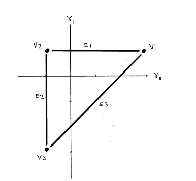
Figure 1. The six boundary components.

Our strategy will be the same as in sections 3-5, but there are significant new aspects, which we summarize briefly now. We begin by giving the value of the matrix $M$ for each boundary component. We shall find the same formulae for the Stokes matrices as in the non-resonant case. However, the connection matrix $D_{1}$ for $\hat{\omega}$ depends very much on the boundary component, and the current section is devoted to computing this. In section 7 we shall use $D_{1}$ to compute the corresponding connection matrix $E_{1}$ for $\hat{\alpha}$. The Iwasawa factorization argument of section 4 does not apply to the boundary points, but we shall use a modified argument based on [7]. This will allow us to calculate $E_{1}$ in the resonant cases. After that (section 8), we shall give the holomorphic and asymptotic data for all local solutions near $t=0$, and characterize the global solutions in terms of this data, as in the non-resonant case.

Let us begin with the canonical solution $\Phi^{(\infty)}(\lambda)=\left(I+O(\tfrac{1}{\lambda})\right)\lambda^{m}\lambda^{M}$ of (3.1) at infinity. In Table 1 we give $m=\operatorname{diag}(m_{0},m_{1},m_{2},m_{3})$ for each of the six components, together with the parameters $a_{1},a_{2},a_{3}$. The latter were introduced in (3.5), and will be convenient here also.

	$(\gamma_{0},\gamma_{1})$	$(m_{0},m_{1},m_{2},m_{3})$	$(a_{1},a_{2},a_{3})$
E1	$(\gamma_{0},1)$	$(m_{0},-\tfrac{1}{2},\tfrac{1}{2},-m_{0})$	$(\tfrac{a}{2},\tfrac{a}{2},a),0\!<\!a\!=\!2m_{0}\!+\!3\!<\!4$
E2	$(-1,\gamma_{1})$	$(\tfrac{1}{2},m_{1},-m_{1},-\tfrac{1}{2})$	$(a,4\!\!-\!\!a,4),0\!<\!a\!=\!\tfrac{3}{2}\!-\!m_{1}\!<\!2$
E3	$(\gamma_{0},\gamma_{0}\!\!-\!\!2)$	$\!(m_{0},m_{0}\!+\!1,-m_{0}\!\!-\!\!1,-m_{0})\!$	$(0,a,a),0\!<\!a\!=\!2m_{0}\!+\!3\!<\!4$
V1	$(3,1)$	$(-\tfrac{3}{2},-\tfrac{1}{2},\tfrac{1}{2},\tfrac{3}{2})$	$(0,0,0)$
V2	$(-1,1)$	$(\tfrac{1}{2},-\tfrac{1}{2},\tfrac{1}{2},-\tfrac{1}{2})$	$(2,2,4)$
V3	$(-1,-3)$	$(\tfrac{1}{2},\tfrac{3}{2},-\tfrac{3}{2},-\tfrac{1}{2})$	$(0,4,4)$

Table 1. The six boundary components.

We shall compute $M$ by comparing $\Phi^{(\infty)}$ with the solution $\Phi^{\text{Frob}}$ of (3.1) which is obtained by applying the Frobenius method to the scalar o.d.e. $\hat{T}_{0}\,\hat{y}_{0}=0$. This is of the form

$$\Phi^{\text{Frob}}=\begin{pmatrix}-&\hat{y}&-\\ -&\hat{P}_{1}\hat{y}&-\\ -&\hat{P}_{2}\hat{y}&-\\ -&\hat{P}_{3}\hat{y}&-\end{pmatrix},\quad\hat{y}=(\hat{y}^{(0)},\hat{y}^{(1)},\hat{y}^{(2)},\hat{y}^{(3)})$$

where the $\hat{P}_{i}$ are the differential operators defined in section 2, and the $\hat{y}^{(i)}$ are of the form

(6.1) $$\begin{pmatrix}\hat{y}^{(0)}\\ \hat{y}^{(1)}\\ \hat{y}^{(2)}\\ \hat{y}^{(3)}\end{pmatrix}=\lambda^{E^{T}}\begin{pmatrix}\lambda^{m_{0}}&&&\\ &\lambda^{m_{1}-1}&&\\ &&\lambda^{m_{2}-2}&\\ &&&\lambda^{m_{3}-3}\end{pmatrix}\begin{pmatrix}f_{0}\\ f_{1}\\ f_{2}\\ f_{3}\end{pmatrix}$$

where $E$ is nilpotent and $f_{0},f_{1},f_{2},f_{3}$ are holomorphic near $\lambda=\infty$.

Proposition 6.1.

We have $\Phi^{\text{\em{Frob}}}=\Phi^{(\infty)}FU$ where $F$ is diagonal and $U$ is unipotent. The nilpotent matrix $M$ in the canonical solution $\Phi^{(\infty)}(\lambda)=\left(I+O(\tfrac{1}{\lambda})\right)\lambda^{m}\lambda^{M}$ is $M=FU\,E\,(FU)^{-1}=FEF^{-1}=-\hat{c}E\hat{c}^{-1}$. The matrices $E$ and $F$ are given in Table 2, and the matrix $U$ is given in the Appendix.

	$E$	$\hat{c}_{0}\hat{c}_{i}^{-1}F_{i}\ (0\leq i\leq 3)$
E1	$E_{1,2}$	$1,\tfrac{1}{2}at^{-\frac{a}{2}},-\tfrac{1}{2}at^{-\frac{a}{2}},\tfrac{1}{4}a^{3}t^{-a}$
E2	$E_{3,0}$	$-4a_{1}a_{2}t^{-4},a_{1}t^{-a},a_{2}(a_{2}\!-\!a_{1})t^{a-4},4a_{1}a_{2}t^{-4}$
E3	$E_{0,1}+E_{2,3}$	$1,-1,a^{2}t^{-a},-a^{2}t^{-a}$
V1	$E_{0,1}+E_{1,2}+E_{2,3}$	$1,-1,1,-1$
V2	$E_{3,0}+E_{1,2}$	$-16t^{-4},2t^{-2},-2t^{-2},16t^{-4}$
V3	$E_{3,0}+E_{0,1}+E_{2,3}$	$16t^{-4},-16t^{-4},16t^{-4},-16t^{-4}$

Table 2. The matrices $E,F$ in Proposition 6.1. $E_{i,j}$ ($0\leq i,j\leq 3$) denotes the matrix with $1$ in the $(i,j)$ position and $0$ elsewhere.

Proof.

We shall just give the details for the case (E1), as the other cases are very similar. Here we have

$$\hat{T}_{0}=(\partial_{\lambda}-m_{0})(\partial_{\lambda}+\tfrac{3}{2})^{2}(\partial_{\lambda}+m_{0}+3)-\tfrac{4^{4}}{N^{4}}\tfrac{z^{4}}{\lambda^{4}}p_{0}p_{1}p_{2}p_{3},$$

with indicial roots $m_{0},-\tfrac{3}{2},-\tfrac{3}{2},-m_{0}-3$. The Frobenius method gives a unique basis of solutions $\hat{y}$ of the form

$$\hat{y}^{(0)} =\lambda^{m_{0}}f_{0}$$

$$\hat{y}^{(1)} =\lambda^{-\frac{3}{2}}f_{1}$$

$$\hat{y}^{(2)} =\lambda^{-\frac{3}{2}}f_{1}\log\lambda+\lambda^{-\frac{3}{2}}f_{2}$$

$$\hat{y}^{(3)} =\lambda^{-m_{0}-3}f_{3}$$

where $f_{i}(\lambda)=1+\sum_{j=1}^{\infty}f_{i,j}\lambda^{-4j}$ for $i=0,1,3$ and $f_{2}(\lambda)=\sum_{j=1}^{\infty}f_{2,j}\lambda^{-4j}$. This assumes that $m_{0}\neq-1,-\tfrac{1}{2},0$. However, as in the interior case, the explicit formula for $g_{0}$ shows that no further logarithms arise for these points. In the notation of (6.1), this shows that $E=E_{1,2}$ (column 1 of Table 2).

Explicit calculation using the differential operators $\hat{P}_{i}$ shows that $\Phi^{\text{Frob}}$ has the form

$$F\left(I+O(\tfrac{1}{\lambda})\right)\lambda^{m}\lambda^{E_{1,2}}U,\quad U=\left(\begin{smallmatrix}\vphantom{-\frac{2}{a}}1\,&&&\\ &1&-\frac{2}{a}&\\ \vphantom{-\frac{2}{a}}&&1&\\ \vphantom{-\frac{2}{a}}&&&1\end{smallmatrix}\right)$$

where

$$F_{0} =1$$

$$F_{1} =\!-\tfrac{N}{4}(zp_{1})^{-1}(-\tfrac{3}{2}-m_{0})=t^{-\frac{a}{2}}\,\hat{c}_{0}^{-1}\hat{c}_{1}\,\tfrac{1}{2}a$$

$$F_{2} =\left(\!-\tfrac{N}{4}\right)^{2}(z^{2}p_{1}p_{2})^{-1}(-\tfrac{3}{2}-m_{0})=t^{-\frac{a}{2}}\,\hat{c}_{0}^{-1}\hat{c}_{2}\,(-\tfrac{1}{2}a)$$

$$F_{3} =\left(\!-\tfrac{N}{4}\right)^{3}(z^{3}p_{1}p_{2}p_{3})^{-1}(-3-2m_{0})(-\tfrac{3}{2}-m_{0})^{2}=t^{-a}\,\hat{c}_{0}^{-1}\hat{c}_{3}\,\tfrac{1}{4}a^{3}.$$

(cf. the proof of Theorem 3.13). This gives the matrix $F$ (column 2 of Table 2).

It follows that $\Phi^{\text{Frob}}=\left(I+O(\tfrac{1}{\lambda})\right)\lambda^{m}\lambda^{M}FU=\Phi^{(\infty)}FU$, with $M=FUE_{1,2}(FU)^{-1}=FE_{1,2}F^{-1}=-\hat{c}E_{1,2}\hat{c}^{-1}$. Thus we have computed $M$ and it has the properties stated in the proposition. ∎

Now we have to modify Lemma 3.3, Lemma 3.5, and Corollary 3.6 to take account of $M$.

Lemma 6.2.

Cyclic symmetry: $d_{4}^{-1}\,\Phi^{(\infty)}(\omega\lambda)\omega^{-M}\omega^{-m}d_{4}=\Phi^{(\infty)}(\lambda)$

Anti-symmetry: $\Delta\,\Phi^{(\infty)}(\omega^{2}\lambda)^{-T}\omega^{2M^{T}}\omega^{2m}\Delta=\Phi^{(\infty)}(\lambda)$

Proof.

If $\Phi^{(\infty)}(\lambda)=(I+O(\tfrac{1}{\lambda}))\lambda^{m}\lambda^{M}$ is the canonical solution, then (cf. Lemma 3.5) $d_{4}^{-1}\Phi^{(\infty)}(\omega\lambda)$ is also a solution of (3.1), hence $d_{4}^{-1}\Phi^{(\infty)}(\omega\lambda)=\Phi^{(\infty)}(\lambda)C$ for some constant $C$. Now,

$$d_{4}^{-1}\Phi^{(\infty)}(\omega\lambda) =d_{4}^{-1}(I+O(\tfrac{1}{\lambda}))\omega^{m}\lambda^{m}\omega^{M}\lambda^{M}$$

$$=(I+O(\tfrac{1}{\lambda}))\lambda^{m}(d_{4}^{-1}\omega^{m})\lambda^{M}\omega^{M}$$

$$=(I+O(\tfrac{1}{\lambda}))\lambda^{m}\lambda^{M}(d_{4}^{-1}\omega^{m})\omega^{M}$$

because $d_{4}^{-1}\omega^{m}$ commutes with $\lambda^{M}$. Hence $C=d_{4}^{-1}\omega^{m}\omega^{M}$, and this gives the cyclic symmetry. Similarly, using $\Delta\lambda^{-2m}\Delta=\lambda^{2m}$ and $\Delta\lambda^{-2M^{T}}\Delta=\lambda^{-2M}$, we have

$$\Delta\,\Phi^{(\infty)}(\omega^{2}\lambda)^{-T} =\Delta(I+O(\tfrac{1}{\lambda}))\omega^{-2m}\lambda^{-m}\omega^{-2M^{T}}\lambda^{-M^{T}}$$

$$=(I+O(\tfrac{1}{\lambda}))\omega^{2m}\lambda^{m}\omega^{-2M}\lambda^{-M}\Delta$$

$$=(I+O(\tfrac{1}{\lambda}))\lambda^{m}\lambda^{M}\Delta\,\omega^{-2m}\omega^{-2M^{T}}$$

where we have used $\omega^{2m}\lambda^{-M}=\lambda^{M}\omega^{2m}$ at the last step. This gives $\Delta\,\Phi^{(\infty)}(\omega^{2}\lambda)^{-T}=\Phi^{(\infty)}(\lambda)\Delta\,\omega^{-2m}\omega^{-2M^{T}}$, which is the anti-symmetry condition. ∎

Lemma 6.3.

Cyclic symmetry: $D_{k+\scriptstyle\frac{1}{2}}=\Pi\,D_{k}\,\omega^{-M}\omega^{-m}d_{4}$

Anti-symmetry: $D_{k+1}=\tfrac{1}{4}d_{4}\,D_{k}{}^{-T}\,\omega^{2M^{T}}\omega^{2m}\Delta$

Proof.

This follows from Lemma 6.2 (cf. the proof of Lemma 3.5). ∎

Corollary 6.4.

Cyclic symmetry: $D_{k}^{-1}(P_{k}P_{k+\frac{1}{4}}\Pi)D_{k}=d_{4}^{-1}\omega^{m}\omega^{M}$

Anti-symmetry: $D_{k}=R_{k}\tfrac{1}{4}d_{4}D_{k}^{-T}\omega^{2M^{T}}\omega^{2m}\Delta$

Proof.

This follows from Lemma 6.3 (cf.  the proof of Corollary 3.6). ∎

The fact that $P_{k}P_{k+\frac{1}{4}}\Pi$ is conjugate to $d_{4}^{-1}\omega^{m}\omega^{M}$ (and hence has the same eigenvalues as $d_{4}^{-1}\omega^{m}$) implies that the Stokes data is given by the same formulae as before. Therefore, no modifications to Theorem 3.7 are needed.

Next we turn to the main task of this section, the calculation of $D_{1}$ in the boundary cases. Proposition 3.9 still gives a solution of $Tg_{0}(s)=0$, but Corollary 3.10 (the $s$-expansion of $g_{0}(s)$) must be modified because $g_{0}(s)$ now has higher order poles.

Recall that if $g_{0}(s)$ is a solution of $Tg_{0}(s)=0$, then $g(\lambda)=\lambda^{m_{0}}g_{0}(s)=\lambda^{m_{0}}g_{0}(t/\lambda)$ is a solution of $\hat{T}_{0}g(\lambda)=0$.

Proposition 6.5.

We have $\lambda^{m_{0}}g_{0}(s)=\tilde{A}_{0}\hat{y}^{(0)}+\tilde{A}_{1}\hat{y}^{(1)}+\tilde{A}_{2}\hat{y}^{(2)}+\tilde{A}_{3}\hat{y}^{(3)}$ where $\tilde{A}_{0},\tilde{A}_{1},\tilde{A}_{2},\tilde{A}_{3}$ are given in terms of $a_{1},a_{2},a_{3}$ in the Appendix.

Proof.

This is a routine calculation using the Laurent expansion of the gamma function. For reference we give the latter at the end of this section as Lemma 6.7. We give the case (E1) in full here, referring to the Appendix for a complete list of results, which are obtained by exactly the same method. In this case we have $a_{1}=a_{2}=\tfrac{1}{2}a_{3}=\tfrac{1}{2}a$, so

$$g_{0}(s)=\int_{c-{\scriptscriptstyle\sqrt{-1}}\,\infty}^{c+{\scriptscriptstyle\sqrt{-1}}\,\infty}\Gamma(-t)\Gamma(\tfrac{a}{8}-t)^{2}\Gamma(\tfrac{a}{4}-t)2^{-8t}s^{4t}dt.$$

Let us write $X=2^{-8}s^{4}$. As in Corollary 3.10, $(-2\pi{\scriptstyle\sqrt{-1}}\,)^{-1}g_{0}(s)$ is equal to the sum of the residues of $\Gamma(-t)\Gamma(\tfrac{a}{8}-t)^{2}\Gamma(\tfrac{a}{4}-t)X^{t}$, which has simple poles at $t=k$, $t=\tfrac{a}{4}+k$ and double poles at $t=\tfrac{a}{8}+k$ ($k=0,1,2,\dots$).

It is well known (and follows from Lemma 6.7) that

$$\Gamma(-t)=\frac{r_{k}}{t-k}+O(1)$$

near $t=k$ where

$$r_{k}=-{(-1)^{k}}/{k!}$$

so the contribution from the poles $t=k$ of $\Gamma(-t)$ is $\sum_{k=0}^{\infty}r_{k}G(k)X^{k}$ where $G(t)=\Gamma(\tfrac{a}{8}-t)^{2}\Gamma(\tfrac{a}{4}-t)$.

Similarly, the contribution from the poles $t=\tfrac{a}{4}+k$ of $\Gamma(\tfrac{a}{4}-t)$ is $\sum_{k=0}^{\infty}r_{k}H(\tfrac{a}{4}+k)X^{\frac{a}{4}+k}$ where $H(t)=\Gamma(-t)\Gamma(\tfrac{a}{8}-t)^{2}$.

To calculate the residues at the double poles $t=\tfrac{a}{8}+k$ of $\Gamma(\tfrac{a}{8}-t)^{2}$ we use the fact (again from Lemma 6.7) that

$$\textstyle\Gamma(\tfrac{a}{8}-t)=\frac{r_{k}}{t-(\frac{a}{8}+k)}+l_{k}+O(t-(\frac{a}{8}+k))$$

near $t=\frac{a}{8}+k$ where

$$l_{k}=r_{k}(\gamma_{\scriptscriptstyle\text{eu}}-h_{k}) h_{k}=1+\tfrac{1}{2}+\cdots+\tfrac{1}{k}$$ with

and $\gamma_{\scriptscriptstyle\text{eu}}$ denotes the Euler-Mascheroni constant. (We put $h_{0}=0$.) Hence

$$\textstyle\Gamma(\frac{a}{8}-t)^{2}=\frac{r_{k}^{2}}{(t-(\frac{a}{8}+k))^{2}}+\frac{2r_{k}l_{k}}{t-(\frac{a}{8}+k)}+O(1).$$

Let us write $F(t)=\Gamma(-t)\Gamma(\tfrac{a}{4}-t)$. Then the Taylor expansion of $F(t)X^{t}$ at $\tfrac{a}{8}+k$ is of the form

$$F(t)X^{t}=x_{k}+y_{k}(t-(\tfrac{a}{8}+k))+O((t-(\tfrac{a}{8}+k))^{2}),$$

where $x_{k}=F(\tfrac{a}{8}+k)X^{\frac{a}{8}+k}$, $y_{k}=F^{\prime}(\tfrac{a}{8}+k)X^{\frac{a}{8}+k}+F(\tfrac{a}{8}+k)X^{\frac{a}{8}+k}\log X$. The residue of $\Gamma(-t)\Gamma(\tfrac{a}{8}-t)^{2}\Gamma(\tfrac{a}{4}-t)X^{t}$ at $\tfrac{a}{8}+k$ is $2r_{k}l_{k}x_{k}+r_{k}^{2}y_{k}=2r_{k}^{2}(\gamma_{\scriptscriptstyle\text{eu}}-h_{k})x_{k}+r_{k}^{2}y_{k}$, and the contribution from the poles $t=\tfrac{a}{8}+k$ is

$$\sum_{k=0}^{\infty}\ 2r_{k}^{2}(\gamma_{\scriptscriptstyle\text{eu}}-h_{k})F(\tfrac{a}{8}+k)X^{\frac{a}{8}+k}+r_{k}^{2}F^{\prime}(\tfrac{a}{8}+k)X^{\frac{a}{8}+k}+r_{k}^{2}F(\tfrac{a}{8}+k)X^{\frac{a}{8}+k}\log X.$$

Summing all three contributions, and multiplying by $\lambda^{m_{0}}$, we obtain a solution of $\hat{T}_{0}\hat{y}=0$, which therefore must be a linear combination of the Frobenius solutions (6.1). Let us write $\lambda^{m_{0}}g_{0}(s)=\tilde{A}_{0}\hat{y}^{(0)}+\tilde{A}_{1}\hat{y}^{(1)}+\tilde{A}_{2}\hat{y}^{(2)}+\tilde{A}_{3}\hat{y}^{(3)}$. Using $X=2^{-8}t^{4}\lambda^{-4}$, and $\log X=\log 2^{-8}t^{4}-4\log\lambda$, by inspection we obtain the formulae for the $\tilde{A}_{i}$ which are listed in the Appendix. ∎

The analysis of equation (3.1) at $\lambda=0$ remains the same as in section 3. Proposition 3.11 and Corollary 3.12 apply equally well to the boundary case, so we may proceed now to the analogue of Theorem 3.13:

Theorem 6.6.

The connection matrix $D_{1}$ is given by the formula

$$D_{1}={\scriptstyle\sqrt{-1}}\,\,\pi^{\frac{5}{2}}\,2^{-2m_{0}+\frac{1}{2}}\,(P\tilde{K})^{-T}\,{\tilde{\Gamma}}{}^{-T}\hat{c}^{-1}$$

where $P,\hat{c}$ are as in Theorem 3.13, and $\tilde{K},\tilde{\Gamma}$ are given in the Appendix. The matrices $P,\tilde{K},\tilde{\Gamma}$ depend on $m$, but not on $\hat{c}$.

Proof.

(i) Expression for $\Phi^{(0)}_{1}$. As in the proof of Theorem 3.13 we have

$$\phi^{(0)}_{1}(\lambda)^{T}=P\begin{pmatrix}j(\omega^{2}\lambda)\\ j(\omega\lambda)\\ j(\lambda)\\ j(\omega^{-1}\lambda))\end{pmatrix},$$

where $j(\lambda)=\kappa_{0}^{-1}\hat{c}_{0}\lambda^{m_{0}}g_{0}(s)$ and $\kappa_{0}={\scriptstyle\sqrt{-1}}\,\pi^{\frac{5}{2}}2^{-2m_{0}+\frac{1}{2}}$. By Proposition 6.5,

$$j(\lambda) =\kappa_{0}^{-1}\hat{c}_{0}(\tilde{A}_{0},\tilde{A}_{1},\tilde{A}_{2},\tilde{A}_{3})\begin{pmatrix}\hat{y}^{(0)}\\ \hat{y}^{(1)}\\ \hat{y}^{(2)}\\ \hat{y}^{(3)}\end{pmatrix}$$

$$=\kappa_{0}^{-1}\hat{c}_{0}(\tilde{A}_{0},\tilde{A}_{1},\tilde{A}_{2},\tilde{A}_{3})\lambda^{E^{T}}\lambda^{m^{\prime}}\begin{pmatrix}f_{0}\\ f_{1}\\ f_{2}\\ f_{3}\end{pmatrix}$$

where $m^{\prime}=(m_{0},m_{1}-1,m_{2}-2,m_{3}-3)$. From this we obtain, for any $k\in\mathbb{Z}$,

$$j(\omega^{k}\lambda)=\kappa_{0}^{-1}\hat{c}_{0}(\tilde{A}_{0},\tilde{A}_{1},\tilde{A}_{2},\tilde{A}_{3})(\omega^{k})^{E^{T}}(\omega^{k})^{m^{\prime}}\begin{pmatrix}\hat{y}^{(0)}\\ \hat{y}^{(1)}\\ \hat{y}^{(2)}\\ \hat{y}^{(3)}\end{pmatrix},$$

as $f_{i}(\omega\lambda)=f_{i}(\lambda)$ and $\lambda^{E^{T}}$ commutes with $\omega^{m^{\prime}}(=d_{4}^{-1}\omega^{m})$.

Let us apply the identity

$$\left(\begin{smallmatrix}\!a_{1},&a_{2},&\dots\,,&a_{r}\!\end{smallmatrix}\right)\left(\begin{smallmatrix}b_{r}&&&\\ \vdots&\ddots&&\\ b_{2}&\ddots&\ddots&\\ b_{1}&b_{2}&\cdots&b_{r}\end{smallmatrix}\right)=\left(\begin{smallmatrix}\!b_{1},&b_{2},&\dots\,,&b_{r}\!\end{smallmatrix}\right)\left(\begin{smallmatrix}a_{r}&&&\\ \vdots&\ddots&&\\ a_{2}&\ddots&\ddots&\\ a_{1}&a_{2}&\cdots&a_{r}\end{smallmatrix}\right)$$

to the term $(\tilde{A}_{0},\tilde{A}_{1},\tilde{A}_{2},\tilde{A}_{3})(\omega^{k})^{E^{T}}$ (when $E^{T}$ is lower triangular; otherwise an analogous identity holds). We obtain

$$(\tilde{A}_{0},\tilde{A}_{1},\tilde{A}_{2},\tilde{A}_{3})(\omega^{k})^{E^{T}}=o_{k}\,\tilde{A}$$

for certain $1\times 4$, $4\times 4$ matrices $o_{k},\tilde{A}$ where $o_{k}$ depends only on $\omega$ (and $k$) and $\tilde{A}$ depends only on $\tilde{A}_{0},\tilde{A}_{1},\tilde{A}_{2},\tilde{A}_{3}$. It follows that

$$\phi^{(0)}_{1}(\lambda)^{T}=\kappa_{0}^{-1}\hat{c}_{0}\,P\tilde{K}\tilde{A}\begin{pmatrix}\hat{y}^{(0)}\\ \hat{y}^{(1)}\\ \hat{y}^{(2)}\\ \hat{y}^{(3)}\end{pmatrix}$$

where

$$\tilde{K}=\begin{pmatrix}-&o_{2}(\omega^{2})^{m^{\prime}}&-\\ -&o_{1}(\omega)^{m^{\prime}}&-\\ -&o_{0}&-\\ -&o_{\!-1}(\omega^{-1})^{m^{\prime}}&-\end{pmatrix}.$$

In this way, we obtain the matrices $\tilde{K},\tilde{A}$ listed in the Appendix.

For example, in the case (E1), where $m^{\prime}=(m_{0},-\tfrac{3}{2},-\tfrac{3}{2},-m_{0}-3)$, we apply the above identity (with $r=2$) to the sub-matrices

$$(\tilde{A}_{1},\tilde{A}_{2})\begin{pmatrix}1&0\\ \log\omega^{k}&1\end{pmatrix}=(\log\omega^{k},1)\begin{pmatrix}\tilde{A}_{2}&0\\ \tilde{A}_{1}&\tilde{A}_{2}\end{pmatrix},$$

and this gives $o_{k}=(1,\log\omega^{k},1,1)$ and $\tilde{A}=\begin{pmatrix}\tilde{A}_{0}&&&\\ &\tilde{A}_{2}&&\\ &\tilde{A}_{1}&\tilde{A}_{2}&\\ &&&\tilde{A}_{3}\end{pmatrix}$.

(ii) Expression for $\Phi^{(\infty)}$. From Proposition 6.1 we have

$$\phi^{(\infty)}(\lambda)^{T}=F^{-1}U^{-T}\phi^{\text{Frob}}(\lambda)^{T}=F^{-1}U^{-T}\begin{pmatrix}\hat{y}^{(0)}\\ \hat{y}^{(1)}\\ \hat{y}^{(2)}\\ \hat{y}^{(3)}\end{pmatrix}.$$

(iii) The computation of $D_{1}$. Inserting the results of (i) and (ii) into $D_{1}^{-T}{\phi^{(\infty)}}(\lambda)^{T}={\phi^{(0)}_{1}}(\lambda)^{T}$, we obtain

$$D_{1}^{-T}=\kappa_{0}^{-1}\hat{c}_{0}\,P\tilde{K}\tilde{A}\,U^{T}\!F=\kappa_{0}^{-1}\,P\tilde{K}\tilde{\Gamma}\hat{c}$$

where $\tilde{\Gamma}=\hat{c}_{0}\tilde{A}\,U^{T}\!F\hat{c}^{-1}$. This gives the stated formula for $D_{1}$. ∎

We end this section by recalling the Laurent expansion of the gamma function, which was used in the proof of Proposition 6.5. (The first two terms suffice for all cases except the vertices (V1) and (V3); in those cases the first four terms are needed.)

Lemma 6.7.

The Laurent expansion of $\Gamma(-t)$ at its simple pole $t=0$ is

$$\Gamma(-t) =-\Gamma(1)t^{-1}+\Gamma^{\prime}(1)-\tfrac{1}{2}\Gamma^{\prime\prime}(1)t+\tfrac{1}{3!}\Gamma^{\prime\prime\prime}(1)t^{2}+O(t^{3})$$

$$=\ \ r_{0}t^{-1}+l_{0}+m_{0}t+n_{0}t^{2}+O(t^{3})$$

where $r_{0}=-1$, $l_{0}=-\gamma_{\scriptscriptstyle\text{eu}}$, $m_{0}=-\tfrac{1}{2}(\gamma_{\scriptscriptstyle\text{eu}}^{2}+\tfrac{1}{6}\pi^{2})$, $n_{0}=\tfrac{1}{6}(-\gamma_{\scriptscriptstyle\text{eu}}^{3}-\tfrac{1}{2}\pi^{2}\gamma_{\scriptscriptstyle\text{eu}}-2\zeta(3))$. Here $\gamma_{\scriptscriptstyle\text{eu}}=\lim_{n\to\infty}\ 1+\tfrac{1}{2}+\cdots+\tfrac{1}{n}-\log n$ (the Euler-Mascheroni constant), and $\zeta(3)=\sum_{k=1}^{\infty}k^{-3}$.

Proof.

This follows from the Taylor expansion $-\Gamma(-t+1)=t\Gamma(-t)=r_{0}+l_{0}t+m_{0}t^{2}+n_{0}t^{3}+O(t^{4})$ together with the well known values of the derivatives of the gamma function at $t=1$. ∎

7. Resonance: the connection matrix for $\hat{\alpha}$

We have to modify the Iwasawa factorization argument in Theorem 4.1. There we assumed $k_{i}>-1$, which allowed us to choose a fundamental solution $L$ such that $L|_{z=0}=I$. But on the boundary we have (some) $k_{i}=-1$, and we need a new argument when this happens.

Proposition 7.1.

There is a unique fundamental solution $L$ of the o.d.e. $L^{-1}L_{z}=\tfrac{1}{\lambda}\eta$ of the form $L=eS$, where

$$e=z^{\frac{1}{\lambda}\Lambda^{T}},\quad\Lambda=-\tfrac{N}{4}M=-\tfrac{N}{4}FEF^{-1},\quad S=I+O(z^{N}/\lambda^{4})$$

with the properties (i) $S|_{z=0}=I$, (ii) $S$ is homogeneous in the sense that the $(i,j)$ entry of $S$ has weight $2(m_{j}-m_{i})$.

Proof.

Substituting $L=eS$ into $L^{-1}L_{z}=\tfrac{1}{\lambda}\eta$, we obtain the equation

$$S^{-1}S_{z}=\tfrac{1}{\lambda}\eta-\tfrac{1}{\lambda}\tfrac{1}{z}S^{-1}\Lambda^{T}S$$

for $S$. Observe that $\eta-\tfrac{1}{z}\Lambda^{T}$ contains only $z^{p}$ with $p>-1$. (For example, in the case (E1), we have $\Lambda=c_{2}E=c_{2}E_{1,2}$ with $k_{2}=-1$ and $k_{i}>-1$ if $i\neq 2$, so $\eta-\tfrac{1}{z}\Lambda^{T}=c_{0}E_{0,3}z^{k_{0}}+c_{1}E_{1,0}z^{k_{1}}+c_{2}E_{2,1}z^{-1}+c_{3}E_{3,2}z^{k_{3}}-c_{2}E_{2,1}z^{-1}=c_{0}E_{0,3}z^{k_{0}}+c_{1}E_{1,0}z^{k_{1}}+c_{3}E_{3,2}z^{k_{3}}$.) Hence there exists a unique solution near $z=0$ with $S|_{z=0}=I$. The coefficients of this equation have the stated homogeneity property, hence $S$ does as well. ∎

Lemma 7.2.

We have $\Phi^{(\infty)}=(\tilde{g}L)^{T}z^{-\Lambda}$ where $\tilde{g}=(\lambda^{m}\lambda^{M})^{T}$.

Proof.

Let $\Phi=(\tilde{g}L)^{T}$ where $\tilde{g}=(\lambda^{m}\lambda^{M})^{T}$. As $\tilde{g}$ is independent of $z$, $\tilde{g}L$ satisfies $(\tilde{g}L)^{-1}(\tilde{g}L)_{z}dz=\tfrac{1}{\lambda}\eta dz=\omega$.

We claim that all entries of the $i$-th column of $\tilde{g}L$ have weight $2m_{i}$. Since $\lambda^{m}z^{\frac{1}{\lambda}\Lambda^{T}}=z^{\Lambda^{T}}\lambda^{m}$, we have

$$\tilde{g}L=\lambda^{M^{T}}\lambda^{m}z^{\frac{1}{\lambda}\Lambda^{T}}S=\lambda^{M^{T}}z^{\Lambda^{T}}\lambda^{m}S.$$

Since the weights of $\lambda,z$ are $2,\tfrac{8}{N}$ respectively, the factor

$$\lambda^{M^{T}}z^{\Lambda^{T}}=z^{\Lambda^{T}}\lambda^{M^{T}}$$

has all (nonzero) entries of weight zero. Hence the entries of $\tilde{g}L$ have the same weights as those of $\lambda^{m}S$. Now, the $(i,j)$ entry of $S$ has weight $2(m_{j}-m_{i})$, and the diagonal elements of $\lambda^{m}$ have weights $2m_{0},2m_{1},2m_{2},2m_{3}$. This justifies the claim.

As in section 2.3, this implies that $(\tilde{g}L)^{-1}(\tilde{g}L)_{\lambda}d\lambda=\hat{\omega}$, i.e. $\Phi=(\tilde{g}L)^{T}$ is a solution of (3.1). On the other hand, we have $(\tilde{g}L)^{T}=S^{T}z^{\frac{1}{\lambda}\Lambda}\lambda^{m}\lambda^{M}=(I+O(z^{N}/\lambda^{4}))\lambda^{m}\lambda^{M}z^{\Lambda}$, so this must be $\Phi^{(\infty)}(\lambda)z^{\Lambda}$. ∎

Now we are ready for the Iwasawa factorization. Recall (section 2) that this means the Iwasawa factorization for the complex loop group $\Lambda\textrm{SL}_{n+1}\mathbb{C}$ with respect to the real form $\Lambda_{\mathbb{R}}\textrm{SL}_{n+1}\mathbb{C}=\{\gamma\in\Lambda\textrm{SL}_{n+1}\mathbb{C}\ |\ c(\gamma(1/{\bar{\lambda}}))=\gamma(\lambda)\}$.

Proposition 7.3.

For each of the boundary cases, there exists a loop $\gamma\in\Lambda\textrm{SL}_{n+1}\mathbb{C}$ with the following properties.

(i) The Iwasawa factorization

$$\gamma L=(\gamma L)_{\mathbb{R}}(\gamma L)_{+}$$

exists near $z=0$.

(ii) The $(i,j)$ entry of $(\gamma L)_{+}$ has weight $2(m_{j}-m_{i})$.

(iii) $(\gamma L)_{+}=\operatorname{diag}(b_{0},b_{1},b_{2},b_{3})+O(\lambda)$ with $b_{0}b_{3}=1=b_{1}b_{2}$.

The loop $\gamma$ and the functions $b_{i}$ are given in Table 3. In general $(\gamma L)_{\mathbb{R}},(\gamma L)_{+}$ are multi-valued, but each $b_{i}$ is a single valued function of $|z|$ near $z=0$.

	$\gamma$	$b_{i}=X_{i}(I+o(1))$ as $z\to 0$; $\ell_{|z|}=\log|z|$
$\left(\begin{smallmatrix}X\\ X\\ X\\ X\\ X\\ X\end{smallmatrix}\right)$ E1	$\left(\begin{smallmatrix}1&&&\\ &\ 1\ &-\lambda&\\ &&1&\\ &&&1\end{smallmatrix}\right)$	$X_{0}=1$, $X_{1}=(1\!-\!2c_{2}\ell_{|z|})^{\frac{1}{2}}$
$\left(\begin{smallmatrix}X\\ X\\ X\\ X\\ X\\ X\end{smallmatrix}\right)$ E3	$\left(\begin{smallmatrix}1\ &-\lambda&&\\ &1&&&\\ &&\ 1\ &-\lambda\\ &&&1\end{smallmatrix}\right)$	$X_{0}=(1\!-\!2c_{1}\ell_{|z|})^{\frac{1}{2}}$, $X_{1}=(1\!-\!2c_{1}\ell_{|z|})^{-\frac{1}{2}}$
$\left(\begin{smallmatrix}X\\ X\\ X\\ X\\ X\\ X\end{smallmatrix}\right)$ V1	see Proof	see Note $1$ for $X_{0},X_{1}$
$\left(\begin{smallmatrix}X\\ X\\ X\\ X\\ X\\ X\end{smallmatrix}\right)$ V2	$\left(\begin{smallmatrix}1&&&\\ &\ 1\ &-\lambda&&\\ &&1&\\ -\lambda&&&\ 1\end{smallmatrix}\right)$	$X_{0}=(1\!-\!2c_{0}\ell_{|z|})^{-\frac{1}{2}},X_{1}=(1\!-\!2c_{2}\ell_{|z|})^{\frac{1}{2}}$

Table 3. The loop $\gamma$ and the functions $b_{i}$ in Proposition 7.3.

Note $1$.  In the case (V1), we have $X_{0}=(-1-c_{2}\ell_{|z|}-2c_{1}c_{2}\ell_{|z|}^{2}-\tfrac{4}{3}c_{1}^{2}c_{2}\ell_{|z|}^{3})^{\frac{1}{2}}$, $X_{0}X_{1}=(-c_{2}c_{1}^{-1}+\tfrac{1}{4}c_{2}^{2}c_{1}^{-2}-(2c_{2}-c_{2}^{2}c_{1}^{-1})\ell_{|z|}+2c_{2}^{2}\ell_{|z|}^{2}+\tfrac{8}{3}c_{1}c_{2}^{2}\ell_{|z|}^{3}+\tfrac{4}{3}c_{1}^{2}c_{2}^{2}\ell_{|z|}^{4})^{\frac{1}{2}}$.

Note $2$.  The tt*-Toda equations have the symmetry $w\mapsto\Delta w\Delta$. In our situation ($n=3$) this means that $(-w_{1},-w_{0})$ is a solution whenever $(w_{0},w_{1})$ is a solution. In terms of Figure 1, this corresponds to reflection in the line $\gamma_{0}+\gamma_{1}=0$. Therefore, regarding the asymptotics of the functions $w_{i}$, it suffices to treat the cases (E1),(E3),(V1),(V2). From now on we restrict to these cases.

Proof.

We use the method of Theorem 4.1 of [7]. We give the details for the case (E1), then state the modifications needed for the other cases.

In general, an Iwasawa factorization $U=U_{\mathbb{R}}U_{+}$ with $U_{+}=b+O(\lambda)$ is equivalent to a Birkhoff factorization $V=V_{-}V_{+}$ for $V=c(U)(1/\bar{\lambda})^{-1}U(\lambda)$, as

$$V=c(U)(1/\bar{\lambda})^{-1}U(\lambda) =c(U_{+})(1/\bar{\lambda})^{-1}c(U_{\mathbb{R}})(1/\bar{\lambda})^{-1}U_{\mathbb{R}}U_{+}$$

$$=c(U_{+})(1/\bar{\lambda})^{-1}U_{+}(\lambda),$$

which can be expressed in the form $V_{-}V_{+}$ with $V_{-}=I+O(1/\lambda)$ and $V_{+}=b^{2}+O(\lambda)$.

First we shall establish the local (near $z=0$) Iwasawa factorization of $Y=\gamma e$, then deduce that of $U=\gamma eS$ $(=\gamma L)$. In the case (E1) we write $\gamma$ (from Table 3) as

$$\gamma=d_{\lambda}^{-1}Ad_{\lambda},\quad A=\left(\begin{smallmatrix}1&&&\\ &1&-1&\\ &&1&\\ &&&1\end{smallmatrix}\right),\quad d_{\lambda}=\left(\begin{smallmatrix}1&&&\\ &\lambda&&\\ &&\lambda^{2}&\\ &&&\!\!\lambda^{3}\end{smallmatrix}\right).$$

Let us introduce

(7.1) $$\Delta_{1}=A^{T}\Delta A^{-T}.$$

We shall make use of the properties

(i) $\gamma$ satisfies the cyclic symmetry and anti-symmetry conditions $\tau(\gamma(\lambda))=\gamma(\omega\lambda)$ and $\sigma(\gamma(\lambda))=\gamma(-\lambda)$, and

(ii) $\Delta_{1}\Lambda=-\Lambda\Delta_{1}$

(both of which are easily verified). The first is needed so that $\gamma L$ lies in the (complex, twisted) loop group that we are using, hence also its Iwasawa and Birkhoff factors. The second will be used in the following paragraph and later in the proof of Proposition 7.7.

Let us now compute $Z=c(\gamma e)(1/\bar{\lambda})^{-1}(\gamma e)(\lambda)$. First we observe that $(\gamma e)(\lambda)=d_{\lambda}^{-1}Ad_{\lambda}\ d_{\lambda}^{-1}z^{\Lambda^{T}}d_{\lambda}=d_{\lambda}^{-1}Az^{\Lambda^{T}}d_{\lambda}$, $c(\gamma e)(1/\bar{\lambda})=\Delta d_{\lambda}A\bar{z}^{\Lambda^{T}}d_{\lambda}^{-1}\Delta$. Hence

$$Z =\Delta d_{\lambda}\bar{z}^{(-\Lambda^{T})}A^{-1}d_{\lambda}^{-1}\Delta\ d_{\lambda}^{-1}Az^{\Lambda^{T}}d_{\lambda}$$

$$=\lambda^{-3}\Delta d_{\lambda}\bar{z}^{(-\Lambda^{T})}A^{-1}\Delta A\ z^{\Lambda^{T}}d_{\lambda}$$

$$=\lambda^{-3}d_{\lambda}^{-1}d_{\lambda}\Delta d_{\lambda}\ \Delta_{1}^{T}\ \bar{z}^{\Lambda^{T}}z^{\Lambda^{T}}d_{\lambda}\quad\text{by (ii) above}$$

$$=d_{\lambda}^{-1}\Delta\,\Delta_{1}^{T}e^{2\log|z|\Lambda^{T}}d_{\lambda}.$$

Inserting the value of $\Delta_{1}$ from (7.1) we obtain

(7.2) $$Z=d_{\lambda}^{-1}{\scriptsize\left(\begin{array}[]{c|cc|c}1&&&\\ \hline\cr&1\!-\!2c_{2}\log|z|&-1&\\ &1&0&\\ \hline\cr&&&1\end{array}\right)}d_{\lambda}.$$

If it exists, the Birkhoff factorization $Z=Z_{-}Z_{+}$ must be of the form

(7.3) $$Z_{-}Z_{+}=d_{\lambda}^{-1}\left(\begin{smallmatrix}\vphantom{X_{0}^{2}}1&\hphantom{X_{0}^{2}}&\hphantom{X_{0}^{2}}&\hphantom{X_{0}^{2}}\\ *&\vphantom{X_{0}^{2}}1&&\\ *&*&\vphantom{X_{0}^{2}}1&\\ *&*&*&\vphantom{X_{0}^{2}}1\end{smallmatrix}\right)d_{\lambda}\ \ d_{\lambda}^{-1}\left(\begin{smallmatrix}X_{0}^{2}&*&*&*\\ &X_{1}^{2}&*&*\\ &&X_{2}^{2}&*\\ &&&X_{3}^{2}\end{smallmatrix}\right)d_{\lambda}.$$

The existence of the factorization (near $z=0$) now follows from an explicit computation of the $X_{i}$ (cf.  [11], Chapter 14, Step 2). This may be done by equating the upper principal $k\times k$ minors of (7.2) and (7.3). By the anti-symmetry condition in (i) above we must have $X_{0}X_{3}=1=X_{1}X_{2}$, so it suffices to do this for $k=1,2$. We obtain

$$X_{0}^{2}=1,\quad X_{0}^{2}X_{1}^{2}=1\!-\!2c_{2}\log|z|,$$

respectively. The fact that these are positive for $z$ close to (but not equal to) zero shows that the Birkhoff factorization $Z=Z_{-}Z_{+}$ exists in some punctured neighbourhood of zero, and hence also the Iwasawa factorization $Y=Y_{\mathbb{R}}Y_{+}$, with single-valued $X_{i}$.

Next, we can deduce the existence of the local (near $z=0$) Iwasawa factorization of $U=\gamma L$. For this we consider

$$V=c(\gamma L)(1/\bar{\lambda})^{-1}(\gamma L)(\lambda)=c(S)(1/\bar{\lambda})^{-1}Z(\lambda)S(\lambda),$$

where $Z(\lambda)=d_{\lambda}^{-1}\Delta\,\Delta_{1}^{T}e^{2\log|z|\Lambda^{T}}d_{\lambda}$ as above.

We claim that $W=Z(\lambda)^{-1}c(S)(1/\bar{\lambda})^{-1}Z(\lambda)S(\lambda)$ is well-defined in a neighbourhood of $z=0$ (including at $z=0$). This follows from the fact that $\lim_{z\to 0}z\log|z|=0$, hence $\lim_{z\to 0}Z(\lambda)^{-1}c(S)(1/\bar{\lambda})^{-1}Z(\lambda)S(\lambda)=I$. Thus we can write

$$c(S)(1/\bar{\lambda})^{-1}Z(\lambda)S(\lambda)=Z(\lambda)W(\lambda)=Z_{-}(\lambda)Z_{+}(\lambda)W(\lambda).$$

As the local (near $z=0$) Birkhoff factorization of $Z_{+}(\lambda)W(\lambda)$ exists, so does that of $Z_{-}(\lambda)Z_{+}(\lambda)W(\lambda)$, and its “positive factor” is of the form $b^{2}=X^{2}(I+o(1))$. This completes the proof for the case (E1).

The cases (E3) and (V2) are very similar. For the case (E3) we take $\gamma=d_{\lambda}^{-1}Ad_{\lambda}$ with

$$A=\left(\begin{smallmatrix}1&-1&&\\ &1&&\\ &&1&-1\\ &&&1\end{smallmatrix}\right),\quad d_{\lambda}=\left(\begin{smallmatrix}1&&&\\ &\lambda&&\\ &&\lambda^{2}&\\ &&&\!\!\lambda^{3}\end{smallmatrix}\right)$$

and for the case (V2)

$$A=\left(\begin{smallmatrix}1&&&\\ &1&-1&\\ &&1&\\ -1&&&1\end{smallmatrix}\right),\quad d_{\lambda}=\left(\begin{smallmatrix}\lambda^{3}&&&\\ &1&&\\ &&\lambda&\\ &&&\lambda^{2}\end{smallmatrix}\right).$$

For the case (V1) we take $d_{\lambda}=\operatorname{diag}(1,\lambda,\lambda^{2},\lambda^{3})$ and any $A$ such that

$$\Delta_{1}=A^{T}\Delta A^{-T}=\begin{pmatrix}1&1&\frac{1}{2}\frac{c_{2}}{c_{1}}&1\\ &1&\frac{c_{2}}{c_{1}}&\frac{1}{2}\frac{c_{2}}{c_{1}}\\ &&1&1\\ &&&1\end{pmatrix}\begin{pmatrix}1&&&\\ &-1&&\\ &&1&\\ &&&-1\end{pmatrix}.$$

This ensures that property (ii) holds, as in the case (V1) case we have $\Lambda=c_{1}E_{0,1}+c_{2}E_{1,2}+c_{1}E_{2,3}$ (Table 2 of section 6). Direct calculation shows that $A$ exists and is essentially unique. ∎

The existence of the Iwasawa factorization allows us to carry out the construction of

$$\alpha=[(\gamma L)_{\mathbb{R}}G]^{-1}d[(\gamma L)_{\mathbb{R}}G]=(w_{t}+\tfrac{1}{\lambda}W^{T})dt+(-w_{{\bar{t}}}+\lambda W)d{\bar{t}},$$

as in section 2.2. Here $w_{0},w_{1},w_{2},w_{3}$ are defined again by $w_{i}=\log b_{i}/|h_{i}|$ but now $b_{0},b_{1},b_{2},b_{3}$ are as in Proposition 7.3 (Table 3).

Using this, we can define $\hat{\alpha}=\left[-\tfrac{t}{\lambda^{2}}\ W^{T}-\tfrac{1}{\lambda}xw_{x}+{\bar{t}}\,W\right]d\lambda$ as in section 2.4.

Lemma 7.4.

Let $\Psi=(\tilde{g}\gamma^{-1}(\gamma L)_{\mathbb{R}}G)^{T}$. Then $\Psi$ satisfies equation (3.2).

Proof.

By definition $[(\gamma L)_{\mathbb{R}}G]^{-1}d[(\gamma L)_{\mathbb{R}}G]=\alpha$. As $\tilde{g}\gamma^{-1}$ is independent of $z$, we have $[\tilde{g}\gamma^{-1}(\gamma L)_{\mathbb{R}}G]^{-1}d[\tilde{g}\gamma^{-1}(\gamma L)_{\mathbb{R}}G]=\alpha$ as well.

We claim that all entries of $\tilde{g}\gamma^{-1}(\gamma L)_{\mathbb{R}}G$ have weight zero. This would imply that $[\tilde{g}\gamma^{-1}(\gamma L)_{\mathbb{R}}G]^{-1}[\tilde{g}\gamma^{-1}(\gamma L)_{\mathbb{R}}G]_{\lambda}d\lambda=\hat{\alpha}$, by the argument of section 2.4.

To prove the claim, we observe that $\tilde{g}\gamma^{-1}(\gamma L)_{\mathbb{R}}(\gamma L)_{+}G=\tilde{g}\gamma^{-1}\gamma LG=\tilde{g}LG=\lambda^{M^{T}}\lambda^{m}z^{\frac{1}{\lambda}\Lambda^{T}}SG=\lambda^{M^{T}}z^{\Lambda}\lambda^{m}SG$. Since $(\gamma L)_{+}G$ and $SG$ have the same weights, so do $\tilde{g}\gamma^{-1}(\gamma L)_{\mathbb{R}}$ and $\lambda^{M^{T}}z^{\Lambda}\lambda^{m}$, and so do $\tilde{g}\gamma^{-1}(\gamma L)_{\mathbb{R}}G$ and $\lambda^{M^{T}}z^{\Lambda}\lambda^{m}G$. The latter has weight zero, so this completes the proof. ∎

The diagram in section 4 must now be modified as follows:

Here $\Phi^{(\infty)}=\Phi^{(0)}_{k}D_{k}$ as in section 3, but now we define $Y_{k}$ and $Z_{k}$ by $\Psi^{(0)}_{k}=(\tilde{g}\gamma^{-1}(\gamma L)_{\mathbb{R}}G)^{T}Y_{k},\quad\Psi^{(\infty)}_{k}=(\tilde{g}\gamma^{-1}(\gamma L)_{\mathbb{R}}G)^{T}Z_{k}$.

Using this we shall obtain the following modification of Theorem 4.1:

Theorem 7.5.

The connection matrix $E_{k}$ is given by the formula

$$E_{k}=\tfrac{1}{4}D_{k}z^{\Lambda}\,\Delta_{1}(\overline{D_{\frac{7}{4}-k}z^{\Lambda}})^{-1}\,d_{4}^{3}\,C,\quad{\scriptsize C=\left(\begin{array}[]{c|ccc}\!\!1&&&\\ \hline\cr&&&1\!\\ &&1&\\ &\!\!1&&\end{array}\right)}$$

where $D_{k}$ is as in section 6 and $\Delta_{1}$ is defined by (7.1). In particular this gives

$$E_{1}=(D_{1}z^{\Lambda})\,\Delta_{1}\,(\overline{D_{1}z^{\Lambda}})^{-1}\,d_{4}^{-1}E_{1}^{\text{\em global}}$$

where $E_{1}^{\text{\em global}}=\tfrac{1}{4}CQ^{(\infty)}_{\frac{3}{4}}$ as in (4.1).

The proof will be given later. It depends on the following modifications of Propositions 4.2 and 4.4.

Proposition 7.6.

$Y_{k}=(D_{k}z^{\Lambda})^{-1}$.

Proof.

This is similar to the proof of Proposition 4.2. We have

$$\Psi^{(0)}_{k} =(\tilde{g}\gamma^{-1}(\gamma L)_{\mathbb{R}}G)^{T}Y_{k}$$

$$=(\tilde{g}\gamma^{-1}(\gamma L)(\gamma L)_{+}^{-1}G)^{T}Y_{k}$$

$$=((\gamma L)_{+}^{-1}G)^{T}(\tilde{g}L)^{T}Y_{k}.$$

Since $(\tilde{g}L)^{T}=\Phi^{(\infty)}z^{\Lambda}=\Phi^{(0)}_{k}D_{k}z^{\Lambda}$, and $\Phi^{(0)}_{k}\sim O_{0}(I+O(\lambda))e^{\frac{t}{\lambda}d_{4}}$, we obtain

$$\Psi^{(0)}_{k} \sim Gb^{-1}O_{0}(I+O(\lambda))e^{\frac{t}{\lambda}d_{4}}D_{k}z^{\Lambda}Y_{k}$$

$$=P_{0}(I+O(\lambda))e^{\frac{t}{\lambda}d_{4}}D_{k}z^{\Lambda}Y_{k}$$

when $\lambda\to 0$. But $\Psi^{(0)}_{k}\sim P_{0}(I+O(\lambda))e^{\frac{t}{\lambda}d_{4}}$, so we conclude that $D_{k}z^{\Lambda}Y_{k}=I$. ∎

Proposition 7.7.

$Z_{k}=\tfrac{1}{4}\Delta_{1}\,\bar{Y}_{\frac{7}{4}-k}\,d_{4}^{3}\,C$, where $\Delta_{1}$ is as in (7.1).

Proof.

This is similar to the proof of Proposition 4.4 From $\Psi^{(0)}_{k}=(\tilde{g}\gamma^{-1}(\gamma L)_{\mathbb{R}}G)^{T}Y_{k}$ we obtain

$$\overline{\Psi^{(0)}_{k}(1/\bar{\lambda})} =\bar{G}\ \overline{(\gamma L)_{\mathbb{R}}(1/\bar{\lambda})}^{T}\ \overline{(\tilde{g}\gamma^{-1})(1/\bar{\lambda})}^{T}\ \bar{Y}_{k}$$

$$=\bar{G}\ \Delta(\gamma L)_{\mathbb{R}}(\lambda)^{T}\Delta\ \overline{(\tilde{g}\gamma^{-1})(1/\bar{\lambda})}^{T}\ \bar{Y}_{k}.$$

From $\Psi^{(\infty)}_{\frac{7}{4}-k}=(\tilde{g}\gamma^{-1}(\gamma L)_{\mathbb{R}}G)^{T}Z_{\frac{7}{4}-k}=G(\gamma L)_{\mathbb{R}}^{T}(\tilde{g}\gamma^{-1})^{T}Z_{\frac{7}{4}-k}$, we obtain

$$(\gamma L)_{\mathbb{R}}^{T}=G^{-1}\Psi^{(\infty)}_{\frac{7}{4}-k}Z_{\frac{7}{4}-k}^{-1}(\tilde{g}\gamma^{-1})^{-T}.$$

Substituting this into the previous formula gives

$$\overline{\Psi^{(0)}_{k}(1/\bar{\lambda})}=\bar{G}\,\Delta\,G^{-1}\ \Psi^{(\infty)}_{\frac{7}{4}-k}(\lambda)\ Z_{\frac{7}{4}-k}^{-1}\ (\tilde{g}\gamma^{-1})^{-T}\Delta\ \overline{(\tilde{g}\gamma^{-1})(1/\bar{\lambda})}^{T}\ \bar{Y}_{k}.$$

Now, we have $\bar{G}\,\Delta\,G^{-1}=\Delta$. Furthermore, we claim that

(7.4) $$(\tilde{g}\gamma^{-1})^{-T}\Delta\ \overline{(\tilde{g}\gamma^{-1})(1/\bar{\lambda})}^{T}=\Delta_{1}.$$

From these two facts we have $\overline{\Psi^{(0)}_{k}(1/\bar{\lambda})}=\Delta\Psi^{(\infty)}_{\frac{7}{4}-k}Z_{\frac{7}{4}-k}^{-1}\Delta_{1}\bar{Y}_{k}$. On the other hand, from (4.3) we know that $\overline{\Psi^{(0)}_{k}(1/\bar{\lambda})}=\Delta\Psi^{(\infty)}_{\frac{7}{4}-k}(\lambda)\,C\,4d_{4}$. Comparing these, we deduce that $C\,4d_{4}=Z_{\frac{7}{4}-k}^{-1}\,\Delta_{1}\,\bar{Y}_{k}$, as required.

It remains to establish (7.4). We have $\tilde{g}=(\lambda^{m}\lambda^{M})^{T}$ and (using the notation of the proof of Proposition 7.3) $\gamma=d_{\lambda}^{-1}Ad_{\lambda}$, $\Delta_{1}=A^{T}\Delta A^{-T}$. Thus the left hand side of (7.4) is

$$\lambda^{-M}\lambda^{-m}(d_{\lambda}A^{T}d_{\lambda}^{-1})\Delta(d_{\lambda}^{-1}A^{-T}d_{\lambda})\lambda^{-m}\lambda^{-M}.$$

Observe that $\lambda^{-m}d_{\lambda}$ commutes with $A^{T}$ in all cases. Thus we obtain $\lambda^{-M}A^{T}\lambda^{-m}d_{\lambda}\ d_{\lambda}^{-1}\Delta d_{\lambda}^{-1}\ d_{\lambda}\lambda^{-m}A^{-T}\lambda^{-M}=\lambda^{-M}A^{T}\lambda^{-m}\Delta\lambda^{-m}A^{-T}\lambda^{-M}=\lambda^{-M}A^{T}\Delta A^{-T}\lambda^{-M}=\lambda^{-M}\Delta_{1}\lambda^{-M}.$ By property (ii) in the proof of Proposition 7.3 this is equal to $\Delta_{1}$, as $M=-\frac{4}{N}\Lambda$. ∎

	$\mathcal{E}$	$\mathcal{F}$	$e^{\mathbb{R}}_{i},f^{\mathbb{R}}_{i}$
$\left(\begin{smallmatrix}X\\ X\\ X\\ X\\ X\\ X\\ X\end{smallmatrix}\right)$ E1	$\left(\begin{smallmatrix}e^{\mathbb{R}}_{1}&&&\\ \vphantom{f_{1}^{\mathbb{R}}}&1&&\\ \vphantom{f_{1}^{\mathbb{R}}}&&1&\\ &&&1/e^{\mathbb{R}}_{1}\end{smallmatrix}\right)$	$\left(\begin{smallmatrix}\vphantom{f_{1}^{\mathbb{R}}}1&&&\\ &\,1\,&f^{\mathbb{R}}_{1}&\\ \vphantom{f_{1}^{\mathbb{R}}}&&\,1\,&\\ \vphantom{f_{1}^{\mathbb{R}}}&&&1\end{smallmatrix}\right)$	$\begin{matrix}e^{\mathbb{R}}_{1}=-\frac{\tilde{A}_{3}F_{3}}{\tilde{A}_{0}F_{0}}\\ f^{\mathbb{R}}_{1}=-\frac{F_{2}}{F_{1}}-2\frac{\tilde{A}_{1}^{\flat}}{\tilde{A}_{2}}\end{matrix}$
$\left(\begin{smallmatrix}X\\ X\\ X\\ X\\ X\\ X\\ X\end{smallmatrix}\right)$ E3	$\left(\begin{smallmatrix}e^{\mathbb{R}}_{1}\,&&&\\ &\,e^{\mathbb{R}}_{1}\,&&\\ &&1/e^{\mathbb{R}}_{1}&\\ &&&\ 1/e^{\mathbb{R}}_{1}\end{smallmatrix}\right)$	$\left(\begin{smallmatrix}1&f_{1}^{\mathbb{R}}&&\\ \vphantom{f_{1}^{\mathbb{R}}}&1&&\\ &&1&f_{1}^{\mathbb{R}}\\ \vphantom{f_{1}^{\mathbb{R}}}&&&\ 1\end{smallmatrix}\right)$	$\begin{matrix}e^{\mathbb{R}}_{1}=\frac{\tilde{A}_{3}F_{2}}{\tilde{A}_{1}F_{0}}\\ f^{\mathbb{R}}_{1}=-\frac{F_{3}}{F_{2}}-\frac{\tilde{A}_{2}^{\flat}}{\tilde{A}_{3}}-\frac{\tilde{A}_{0}^{\flat}}{\tilde{A}_{1}}\end{matrix}$
$\left(\begin{smallmatrix}X\\ X\\ X\\ X\\ X\\ X\\ X\end{smallmatrix}\right)$ V1	I	$\left(\begin{smallmatrix}1&\ f_{1}^{\mathbb{R}}\ &\frac{1}{2}(f_{1}^{\mathbb{R}})^{2}&f_{2}^{\mathbb{R}}\\ \vphantom{f_{1}^{\mathbb{R}}}&1&f_{1}^{\mathbb{R}}&\frac{1}{2}(f_{1}^{\mathbb{R}})^{2}\\ &&1&f_{1}^{\mathbb{R}}\\ \vphantom{f_{1}^{\mathbb{R}}}&&&\ 1\end{smallmatrix}\right)$	$\begin{matrix}f^{\mathbb{R}}_{1}=\frac{F_{1}}{F_{0}}-2\frac{\tilde{A}^{\flat}_{2}}{\tilde{A}_{3}}\\ f^{\mathbb{R}}_{2}=\text{see Note}\end{matrix}$
$\left(\begin{smallmatrix}X\\ X\\ X\\ X\\ X\\ X\end{smallmatrix}\right)$ V2	I	$\left(\begin{smallmatrix}\vphantom{f_{1}^{\mathbb{R}}}1&&&\\ \vphantom{f_{1}^{\mathbb{R}}}&\,1\,&f^{\mathbb{R}}_{1}&\\ \vphantom{f_{1}^{\mathbb{R}}}&&\,1\,&\\ f^{\mathbb{R}}_{2}&&&1\end{smallmatrix}\right)$	$\begin{matrix}f^{\mathbb{R}}_{1}&=-\frac{F_{2}}{F_{1}}-2\frac{\tilde{A}_{1}^{\flat}}{\tilde{A}_{2}}\\ f^{\mathbb{R}}_{2}&=-\frac{F_{0}}{F_{3}}-2\frac{\tilde{A}_{3}^{\flat}}{\tilde{A}_{0}}\end{matrix}$

Table 4. The matrices $\mathcal{E},\mathcal{F}$ in Theorem 7.8.

Note.  In the case (V1), we have

$$f^{\mathbb{R}}_{2}=\tfrac{F_{3}}{F_{0}}-\tfrac{(F_{1})^{2}}{(F_{0})^{2}}\tfrac{\tilde{A}_{2}^{\flat}}{\tilde{A}_{3}}+2\tfrac{F_{1}}{F_{0}}\tfrac{(\tilde{A}_{2}^{\flat})^{2}}{(\tilde{A}_{3})^{2}}-2\tfrac{(\tilde{A}_{2}^{\flat})^{3}}{(\tilde{A}_{3})^{3}}+2\tfrac{\tilde{A}_{1}^{\flat}\tilde{A}_{2}^{\flat}}{(\tilde{A}_{3})^{2}}-2\tfrac{\tilde{A}_{0}^{\flat}}{\tilde{A}_{3}}.$$

Proof of Theorem 7.5.   From Propositions 7.6 and 7.7 we have $E_{k}=Y_{k}^{-1}Z_{k}=(z^{-\Lambda}D_{k}^{-1})^{-1}\tfrac{1}{4}\Delta_{1}\overline{z^{-\Lambda}D_{\frac{7}{4}-k}^{-1}}d_{4}^{3}\,C$. This is the required formula for $E_{k}$. We deduce the formula for $E_{1}$ exactly as in the proof of Theorem 4.1 (the generic case). ∎

In view of Theorem 7.5, let us introduce the notation

$$D_{1}^{\flat}=D_{1}z^{\Lambda}.$$

Explicitly, using Theorem 6.6, this gives

$$D_{1}^{\flat} =\kappa_{0}\hat{c}_{0}^{-1}(P\tilde{K})^{-T}(\tilde{A})^{-T}(FU)^{-1}z^{\Lambda}$$

$$=\kappa_{0}\hat{c}_{0}^{-1}(P\tilde{K})^{-T}(\tilde{A})^{-T}z^{-\frac{N}{4}E}(FU)^{-1}$$

because $\Lambda=-\frac{N}{4}M=-\frac{N}{4}(FU)E(FU)^{-1}$ (Proposition 6.1).

Introducing the analogous notation

(7.5) $$\tilde{A}^{\flat}=\tilde{A}z^{\frac{N}{4}E^{T}}U^{T},$$

we can write $D_{1}^{\flat}=\kappa_{0}\hat{c}_{0}^{-1}(P\tilde{K})^{-T}(\tilde{A}^{\flat})^{-T}F^{-1}.$ The matrices $\tilde{A}_{i}^{\flat}$ are listed in the Appendix. They are independent of $z$. It follows that the connection matrices $E_{k}$ are (as expected) independent of $z$.

Theorem 7.8.

The connection matrix $E_{1}$ is given by the formula

$$E_{1}=(P\tilde{K})^{-T}\mathcal{E}\mathcal{F}(P\tilde{K})^{T}\ E_{1}^{\text{\em{global}}}$$

where the diagonal matrix $\mathcal{E}$ and the unipotent matrix $\mathcal{F}$ are are given in Table 4.

Proof.

Let us substitute ($D_{1}^{\flat}=$) $D_{1}z^{\Lambda}=\kappa_{0}\hat{c}_{0}^{-1}\,(P\tilde{K})^{-T}(\tilde{A}^{\flat})^{-T}F^{-1}$ (see above) into $E_{1}=(D_{1}z^{\Lambda})\,\Delta_{1}\,(\overline{D_{1}z^{\Lambda}})^{-1}\,d_{4}^{-1}E_{1}^{\text{global}}$ (Theorem 7.5). Noting that $\kappa_{0}$ and $\tilde{A}^{\flat}$ are pure imaginary, we obtain

$$E_{1}=(P\tilde{K})^{-T}(\tilde{A}^{\flat})^{-T}F^{-1}\Delta_{1}F(\tilde{A}^{\flat})^{T}(\overline{P\tilde{K}})^{T}\,d_{4}^{-1}E_{1}^{\text{global}}.$$

Now, by direct calculation we have

(7.6) $$\bar{\tilde{K}}=-d_{4}\tilde{K}\Delta_{0}$$

where the (symmetric) matrix $\Delta_{0}$ is given in the Appendix. Hence

$$E_{1}=-(P\tilde{K})^{-T}(\tilde{A}^{\flat})^{-T}F^{-1}\Delta_{1}F(\tilde{A}^{\flat})^{T}\Delta_{0}\tilde{K}^{T}d_{4}\bar{P}^{T}d_{4}^{-1}E_{1}^{\text{global}}.$$

As in the proof of Theorem 4.5 we have $d_{4}\bar{P}^{T}d_{4}^{-1}=P^{T}$, so

$$E_{1} =-(P\tilde{K})^{-T}(\tilde{A}^{\flat})^{-T}F^{-1}\Delta_{1}F(\tilde{A}^{\flat})^{T}\Delta_{0}(P\tilde{K})^{T}\,E_{1}^{\text{global}}$$

$$=-(P\tilde{K})^{-T}X^{T}(P\tilde{K})^{T}\,E_{1}^{\text{global}}$$

where $X=\Delta_{0}(\tilde{A}^{\flat})F\Delta_{1}^{T}F^{-1}(\tilde{A}^{\flat})^{-1}$.

It is now straightforward to write $-X^{T}$ as $\mathcal{E}\mathcal{F}$, where $\mathcal{E},\mathcal{F}$ are as stated in Table 4. For example, in the case (E1), we have

$$\Delta_{0}\!=\!\left(\begin{smallmatrix}\vphantom{\tilde{A}_{0}}&&&1\\ \vphantom{\tilde{A}_{0}}&-1&&\\ \vphantom{\tilde{A}_{0}}&\ &1&\\ \vphantom{\tilde{A}_{0}}1&&&\end{smallmatrix}\right)\!,\Delta_{1}\!=\!\left(\begin{smallmatrix}\vphantom{\tilde{A}_{0}}&&&1\\ \vphantom{\tilde{A}_{0}}&-1&1&\\ \vphantom{\tilde{A}_{0}}&\ &1&\\ \vphantom{\tilde{A}_{0}}1&&&\end{smallmatrix}\right)\!,\tilde{A}^{\flat}\!=\!\left(\begin{smallmatrix}\tilde{A}_{0}&&&\\ &\tilde{A}_{2}&&\\ &\tilde{A}_{1}^{\flat}&\tilde{A}_{2}&\\ &&&\tilde{A}_{3}\end{smallmatrix}\right)\!,$$

hence $X$ is of the form $\left(\begin{smallmatrix}*&&&\\ &*&&\\ &*&*&\\ &&&*\end{smallmatrix}\right),$ from which the expressions in Table 4 for $e_{1}^{\mathbb{R}},f_{1}^{\mathbb{R}}$ are obtained. ∎

8. Resonance: the global solutions and their asymptotics

As in the non-resonant case, the Iwasawa factorization (Proposition 7.3) leads to asymptotic expressions for the solutions $w_{i}$ which are smooth near $t=0$. We still have $w_{i}=\log b_{i}/|h_{i}|$ with $|h_{i}|=|\hat{c}_{i}t^{m_{i}}|=|\hat{c}_{i}t^{-\gamma_{i}/2}|$, but now there is an extra term as we have $b_{i}=X_{i}(1+o(1))$ instead of $b_{i}=1+o(1)$. We obtain:

(8.1) $$2w_{i}(t)=\gamma_{i}\log|t|+\log X_{i}^{2}\hat{c}_{i}^{-2}+o(1)$$

as $t\to 0$, where $X_{i}$ is given in Table 3 (section 7). If $X_{i}$ is constant (as in the non-resonant case), the error term $o(1)$ is sufficient to ensure that we have obtained a parametrization of such solutions. If $X_{i}$ is not constant it is necessary to improve the error term. This can be done by examining the proof of Proposition 7.3 more carefully — the error comes from neglecting the factor $Z^{-1}c(S)(1/\bar{\lambda})^{-1}ZS$, and is always of the form $\epsilon=O(|t|^{k}\log^{\ell}|t|)$ for some $k,\ell>0$. The precise values of $k,\ell>0$ will not play any role so we omit them below.

The global solutions are our main interest, and, at this point, we have at our disposal all necessary information about them. First, Theorems 7.5 and 7.8 provide the following analogue of Corollary 5.1:

Corollary 8.1.

The following conditions (i)-(iii) are equivalent:

(i) $E_{1}=\tfrac{1}{4}CQ^{(\infty)}_{\frac{3}{4}}(=E_{1}^{\text{\em global}})$

(ii) $\mathcal{E}=I=\mathcal{F}$ (i.e. all $e_{i}^{\mathbb{R}}=1$ and all $f_{i}^{\mathbb{R}}=0$)

(iii) $D_{1}z^{\Lambda}=d_{4}\overline{D_{1}z^{\Lambda}}\Delta_{1}$ (i.e. $D_{1}^{\flat}=d_{4}\bar{D}_{1}^{\flat}\Delta_{1}$)

As in the non-resonant case, we may use this criterion to give explicitly the holomorphic data and asymptotic data of the global solutions.

We shall discuss the case (E1) in detail, then state the results for the other cases, which are obtained in exactly the same way.

As explained above, from (8.1) and Table 3 we obtain

(8.2) $$\begin{cases}2w_{0}(t)&=\gamma_{0}\log|t|+\log\hat{c}_{0}^{-2}+o(1)\\ 2w_{1}(t)&=\log|t|+\log\left(1-2c_{2}\log|z|\right)\hat{c}_{1}^{-2}+\epsilon\end{cases}$$

as $t\to 0$. Note that $\gamma_{1}=1$ for the second formula as we are in the case (E1). We can rewrite

$$(1-2c_{2}\log|z|)\hat{c}_{1}^{-2} =\hat{c}_{1}^{-2}-\tfrac{N}{2}\log|z|\quad\text{as $\hat{c}_{1}^{-2}=\tfrac{N}{4c_{2}}$ by (\ref{chat})}$$

$$=\hat{c}_{1}^{-2}-2\log\tfrac{|t|}{4}+\tfrac{1}{2}\log\tfrac{c}{N^{4}}\quad\text{as $t=\tfrac{4}{N}\,c^{\frac{1}{4}}\,z^{\frac{N}{4}}$}$$

and then the second formula of (8.2) becomes

$$2w_{1}(t)=\log|t|+\log\left(\hat{c}_{1}^{-2}-2\log\tfrac{|t|}{4}+\tfrac{1}{2}\log\tfrac{c}{N^{4}}\right)+\epsilon.$$

In order to apply Corollary 8.1, we shall convert $\hat{c}_{0}^{-2},\hat{c}_{1}^{-2}$ into monodromy data. The monodromy data is given in Table 4 of section 7. Using the formulae there, with the explicit values of the matrices $F$ (Table 2 of section 6) and $\tilde{A}$ (Appendix), we obtain:

(8.3) $$\begin{cases}e^{\mathbb{R}}_{1}&=-\frac{\tilde{A}_{3}F_{3}}{\tilde{A}_{0}F_{0}}=-2^{-2a}t^{a}\frac{H(\frac{a}{4})}{G(0)}\ \tfrac{1}{4}a^{3}t^{-a}\hat{c}_{0}^{-2}=-\hat{c}_{0}^{-2}2^{-2-2a}a^{3}\frac{H(\frac{a}{4})}{G(0)}\\ f^{\mathbb{R}}_{1}&=-\frac{F_{2}}{F_{1}}-2\frac{\tilde{A}_{1}^{\flat}}{\tilde{A}_{2}}=\hat{c}_{1}^{-2}+\gamma_{\scriptscriptstyle\text{eu}}+\tfrac{4}{a}+\tfrac{1}{2}(\log F)^{\prime}(\tfrac{a}{8})+\tfrac{1}{2}\log\tfrac{c}{N^{4}}\end{cases}$$

These allow us to convert the asymptotic formulae (8.2) into

(8.4) $$\begin{cases}2w_{0}(t)&\!\!\!=\!\gamma_{0}\log|t|+\log\left(-e_{1}^{\mathbb{R}}\,2^{2+2a}a^{-3}G(0)/H(\tfrac{a}{4})\right)+o(1)\\ 2w_{1}(t)&\!\!\!=\!\log|t|\!+\!\log\left(f_{1}^{\mathbb{R}}\!-\!\gamma_{\scriptscriptstyle\text{eu}}\!-\!\tfrac{4}{a}\!-\!\tfrac{1}{2}(\log F)^{\prime}(\tfrac{a}{8})\!-\!2\log\tfrac{|t|}{4}\right)\!+\!\epsilon\end{cases}$$

For the global solutions we have (by (ii) of Corollary 8.1) $e_{1}^{\mathbb{R}}=1$ and $f_{1}^{\mathbb{R}}=0$. Substituting these values into (8.4), we obtain the asymptotics of the global solutions. The holomorphic data of the global solutions (represented by $\hat{c}_{0},\hat{c}_{1}$ in this case) can also be found by putting $e_{1}^{\mathbb{R}}=1$ and $f_{1}^{\mathbb{R}}=0$ in (8.3). This completes our treatment of the case (E1).

For the other cases, exactly the same procedure — taking the explicit data from Tables 2, 3, 4, and the Appendix — gives the holomorphic data and asymptotic data listed in the two corollaries below.

We recall that the original form of the holomorphic data (Definition 2.2) was $p_{i}(z)=c_{i}z^{k_{i}}=c_{i}z^{\alpha_{i}}/z$ ($0\leq i\leq 3$), and that this was transformed into diagonal matrices $\hat{c},m$ in Definition 2.3. Explicit formulae are given in (2.8), (2.10), and Proposition 4.7. We use the data $\hat{c},m$ below.

Corollary 8.2.

(Holomorphic data for global solutions in the resonant cases) The holomorphic data $\hat{c}$ (for the corresponding range of $m$) is listed below. Edges and vertices refer to Figure 1 in section 6.

(E1) $(m_{0},m_{1})=(\tfrac{a}{2}-\tfrac{3}{2},-\tfrac{1}{2})$, $0<a<4$ (top edge)

$\hat{c}_{0}^{2}=-2^{-2-2a}a^{3}H(\tfrac{a}{4})/G(0)$

$\hat{c}_{1}^{-2}=-\gamma_{\scriptscriptstyle\text{eu}}-\tfrac{4}{a}-\tfrac{1}{2}(\log F)^{\prime}(\tfrac{a}{8})-\tfrac{1}{2}\log\tfrac{c}{N^{4}}$

(E3) $(m_{0},m_{1})=(\tfrac{a}{2}-\tfrac{3}{2},\tfrac{a}{2}-\tfrac{1}{2})$, $0<a<4$ (diagonal edge)

$\hat{c}_{0}\hat{c}_{1}=2^{-2a}a^{2}Q(\tfrac{a}{4})/P(0)$

$\hat{c}_{1}\hat{c}_{0}^{-1}=-\gamma_{\scriptscriptstyle\text{eu}}-\tfrac{2}{a}-\tfrac{1}{4}(\log P)^{\prime}(0)-\tfrac{1}{4}(\log Q)^{\prime}(\tfrac{a}{4})-\tfrac{1}{2}\log\tfrac{c}{N^{4}}$

(V1) $(m_{0},m_{1})=(-\tfrac{3}{2},-\tfrac{1}{2})$ (top right vertex)

$\hat{c}_{0}^{-1}\hat{c}_{1}=2\gamma_{\scriptscriptstyle\text{eu}}+\tfrac{1}{2}\log\tfrac{c}{N^{4}}$

$\hat{c}_{0}^{-2}=\tfrac{4}{3}\gamma_{\scriptscriptstyle\text{eu}}^{3}+\tfrac{1}{24}\zeta(3)+\gamma_{\scriptscriptstyle\text{eu}}^{2}\log\tfrac{c}{N^{4}}+\tfrac{1}{4}\gamma_{\scriptscriptstyle\text{eu}}\log^{2}\tfrac{c}{N^{4}}+\tfrac{1}{48}\log^{3}\tfrac{c}{N^{4}}$

(V2) $(m_{0},m_{1})=(\tfrac{1}{2},-\tfrac{1}{2})$ (top left vertex)

$\hat{c}_{0}^{2}=-\gamma_{\scriptscriptstyle\text{eu}}-2-\tfrac{1}{2}(\log S)^{\prime}(1)-\tfrac{1}{2}\log\tfrac{c}{N^{4}}$

$\hat{c}_{1}^{-2}=-\gamma_{\scriptscriptstyle\text{eu}}-1-\tfrac{1}{2}(\log T)^{\prime}(\tfrac{1}{2})-\tfrac{1}{2}\log\tfrac{c}{N^{4}}$

The (products of) gamma functions $F,G,H,\dots$ appearing here are defined in the Appendix.

Finally we reach our goal, the asymptotic data. Recall that all local solutions $w$ near $t=0$ have the leading term asymptotics $2w(t)\sim\gamma\log|t|$. In the non-resonant case we have $2w(t)\sim\gamma\log|t|+\rho$, and the diagonal matrices $\gamma,\rho$ parametrize all such solutions. Therefore, for global solutions, the parameter $\rho$ is determined by $\gamma$, and we gave an explicit formulae for it in Corollary 5.3. In the resonant cases, we have:

Corollary 8.3.

(Asymptotic data for global solutions in the resonant cases) The asymptotics at zero of the global solutions (for the corresponding range of $\gamma$) are listed below. Edges and vertices refer to Figure 1 in section 6. We use the notation $\psi=(\log\Gamma)^{\prime}=\Gamma^{\prime}/\Gamma$ and $\epsilon=O(|t|^{k}\log^{\ell}|t|)$ for some $k,\ell>0$.

(E1) $-1<\gamma_{0}<3,\gamma_{1}=1$ (top edge)

$$2w_{0}(t) \!=\!\gamma_{0}\log|t|+\log\left(-2^{2+2a}a^{-3}G(0)/H(\tfrac{a}{4})\right)+o(1)$$

$$\!=\!\gamma_{0}\log|t|+\log\left(2^{-2\gamma_{0}}\Gamma(\tfrac{3-\gamma_{0}}{4})\Gamma(\tfrac{3-\gamma_{0}}{8})^{2}\Gamma(\tfrac{\gamma_{0}+1}{4})^{-1}\Gamma(\tfrac{\gamma_{0}+5}{8})^{-1}\right)+o(1)$$

$$2w_{1}(t) \!=\!\log|t|+\log\left(-\gamma_{\scriptscriptstyle\text{eu}}\!-\!\tfrac{4}{a}\!-\!\tfrac{1}{2}(\log F)^{\prime}(\tfrac{a}{8})\!-\!2\log\tfrac{|t|}{4}\right)+\epsilon$$

$$\!=\!\log|t|+\log\left(-\gamma_{\scriptscriptstyle\text{eu}}\!-\!\tfrac{4}{3-\gamma_{0}}\!+\!\tfrac{1}{2}\psi(\tfrac{\gamma_{0}-3}{8})\!+\!\tfrac{1}{2}\psi(\tfrac{3-\gamma_{0}}{8})\!-\!2\log\tfrac{|t|}{4}\right)+\epsilon$$

(E3) $-1<\gamma_{0}<3,\gamma_{1}=\gamma_{0}-2$ (diagonal edge)

$$2(w_{0}+w_{1})(t) \!=\!(\gamma_{0}\!+\!\gamma_{1})\log|t|-2\log\left(2^{-2a}a^{2}Q(\tfrac{a}{4})/P(0)\right)+o(1)$$

$$=(\gamma_{0}\!+\!\gamma_{1})\log|t|-2\log\left(2^{2\gamma_{0}-2}\Gamma(\tfrac{\gamma_{0}+1}{4})^{2}\Gamma(\tfrac{3-\gamma_{0}}{4})^{2}\right)+o(1)$$

$$2( w_{0}-w_{1})(t)$$

$$\!=\!2\log|t|\!+\!2\log\left(\!-\gamma_{\scriptscriptstyle\text{eu}}\!-\!\tfrac{2}{a}\!-\!\tfrac{1}{4}(\log P)^{\prime}(0)\!-\!\tfrac{1}{4}(\log Q)^{\prime}(\tfrac{a}{4})\!-\!2\log\tfrac{|t|}{4}\right)+\epsilon$$

$$\!=\!2\log|t|\!+\!2\log\left(\!-\gamma_{\scriptscriptstyle\text{eu}}\!-\!\tfrac{2}{3-\gamma_{0}}\!+\!\tfrac{1}{2}\psi(\tfrac{3-\gamma_{0}}{4})\!+\!\tfrac{1}{2}\psi(\tfrac{\gamma_{0}-3}{4})\!-\!2\log\tfrac{|t|}{4}\right)+\epsilon$$

(V1) $\gamma_{0}=3,\gamma_{1}=1$ (top right vertex)

$2w_{0}(t)=3\log|t|+\log\left(-\tfrac{1}{24}\zeta(3)-\tfrac{4}{3}\gamma_{\scriptscriptstyle\text{eu}}^{3}-4\gamma_{\scriptscriptstyle\text{eu}}^{2}\log\tfrac{|t|}{4}-4\gamma_{\scriptscriptstyle\text{eu}}\log^{2}\tfrac{|t|}{4}\right.$
$\left.\quad-\tfrac{4}{3}\log^{3}\tfrac{|t|}{4}\right)+\epsilon$

$2(w_{0}+w_{1})(t)=4\log|t|+\log\left(\vphantom{\log\tfrac{|t|}{4}}\!\!\!-\!\!\tfrac{1}{12}\gamma_{\scriptscriptstyle\text{eu}}\zeta(3)+\tfrac{4}{3}\gamma_{\scriptscriptstyle\text{eu}}^{4}+(\tfrac{16}{3}\gamma_{\scriptscriptstyle\text{eu}}^{3}-\tfrac{1}{12}\zeta(3))\log\tfrac{|t|}{4}\right.$
$\left.\quad+8\gamma_{\scriptscriptstyle\text{eu}}^{2}\log^{2}\tfrac{|t|}{4}+\tfrac{16}{3}\gamma_{\scriptscriptstyle\text{eu}}\log^{3}\tfrac{|t|}{4}+\tfrac{4}{3}\log^{4}\tfrac{|t|}{4}\right)+\epsilon$

(V2) $\gamma_{0}=-1,\gamma_{1}=1$ (top left vertex)

$$2w_{0}(t) =-\log|t|-\log\left(-\gamma_{\scriptscriptstyle\text{eu}}-2-\tfrac{1}{2}(\log S)^{\prime}(1)-2\log\tfrac{|t|}{4}\right)+\epsilon\ \ \ \ \ \ \ \$$

$$=-\log|t|-\log\left(-2\gamma_{\scriptscriptstyle\text{eu}}+2\log 2-2\log|t|\right)+\epsilon$$

$$2w_{1}(t) =\log|t|+\log\left(-\gamma_{\scriptscriptstyle\text{eu}}-1-\tfrac{1}{2}(\log T)^{\prime}(\tfrac{1}{2})-2\log\tfrac{|t|}{4}\right)+\epsilon$$

$$=\log|t|+\log\left(-2\gamma_{\scriptscriptstyle\text{eu}}+2\log 2-2\log|t|\right)+\epsilon$$

This list covers all resonant cases for which $\gamma_{0}+\gamma_{1}\geq 0$. The remaining cases (E2),(V3) have $\gamma_{0}+\gamma_{1}<0$. The asymptotics for these cases may be obtained by applying the transformation $(w_{0},w_{1})\mapsto(-w_{1},-w_{0})$ (see Note $2$ following Table 3). In the case (V2) we have $\gamma_{0}+\gamma_{1}=0$ and in fact $w_{0}(t)+w_{1}(t)=0$ for all $t$, so our p.d.e. reduces to the sinh-Gordon equation $(w_{0})_{{t\bar{t}}}=\sinh(4w_{0})$, for which the asymptotics given above are well known.

We remark that the normalization constants $c,N$ in the formulae (8.3) and (8.4) for local solutions cancel out in the asymptotics of the global solutions (as they should). The appearance of $c,N$ in (8.3) and (8.4) reflects the fact that our parametrization of the local solutions depends on our conventions for the Iwasawa factorization.

The asymptotics as $t\to\infty$ of all solutions (including the resonant cases) were stated at the end of section 5. Thus we have solved the connection problem (to find the explicit relation between asymptotic data at zero and infinity) also in the resonant cases.

9. Appendix

We list the matrices $\tilde{K},U,\tilde{A}$ appearing in the formula

$$D_{1}=\kappa_{0}\,(P\tilde{K})^{-T}\,\tilde{\Gamma}^{-T}\hat{c}^{-1}=\kappa_{0}\,\hat{c}_{0}^{-1}\,(P\tilde{K})^{-T}(\tilde{A}U^{T}F)^{-T}$$

of Theorem 6.6. Here $\kappa_{0}={\scriptstyle\sqrt{-1}}\,\,\pi^{\frac{5}{2}}\,2^{-2m_{0}+\frac{1}{2}}$, $\hat{c}$ is given in (2.8), and $F$ is given in Table 2. We also list the matrices $\Delta_{0}$ and $\tilde{A}^{\flat}=\tilde{A}z^{\frac{N}{4}E^{T}}U^{T}$ appearing in the formula

$$E_{1}=(P\tilde{K})^{-T}\mathcal{E}\mathcal{F}(P\tilde{K})^{T}E_{1}^{\text{{global}}},\quad\mathcal{E}\mathcal{F}=-(\tilde{A}^{\flat})^{-T}F^{-1}\Delta_{1}F(\tilde{A}^{\flat})^{T}\Delta_{0}$$

of Theorem 7.8. As explained in Note $2$ following Theorem 7.3, we restrict to the cases (E1),(E3),(V1),(V2). To save space we use the abbreviation

$$\ell_{\omega}=\log\omega=\tfrac{1}{2}{{\scriptscriptstyle\sqrt{-1}}\,\pi}$$

here.

Formulae for the case (E1)

$\tilde{K}=\left(\begin{smallmatrix}\vphantom{\tfrac{1}{2}}\omega^{2m_{0}}&\omega^{-3}2\ell_{\omega}&\omega^{-3}&\omega^{-2m_{0}-6}\\ \vphantom{\tfrac{1}{2}}\omega^{m_{0}}&\omega^{-\frac{3}{2}}\ell_{\omega}&\omega^{-\frac{3}{2}}&\omega^{-m_{0}-3}\\ \vphantom{\tfrac{1}{2}}1&0&1&1\\ \vphantom{\tfrac{1}{2}}\omega^{-m_{0}}&\omega^{\frac{3}{2}}(-\ell_{\omega})&\omega^{\frac{3}{2}}&\omega^{m_{0}+3}\end{smallmatrix}\right)$  $U=\left(\begin{smallmatrix}\vphantom{\tfrac{1}{2}}1&&&\\ \vphantom{\tfrac{1}{2}}&\ 1\ &-\frac{2}{a}&\\ \vphantom{\tfrac{1}{2}}&&1&\\ \vphantom{\tfrac{1}{2}}&&&1\end{smallmatrix}\right)$

$\tilde{A}=\left(\begin{smallmatrix}\vphantom{\tfrac{1}{2}}\tilde{A}_{0}&&&\\ \vphantom{\tfrac{1}{2}}&\tilde{A}_{2}&&\\ \vphantom{\tfrac{1}{2}}&\tilde{A}_{1}&\tilde{A}_{2}&\\ \vphantom{\tfrac{1}{2}}&&&\tilde{A}_{3}\end{smallmatrix}\right)$  $\tilde{A}^{\flat}=\left(\begin{smallmatrix}\vphantom{\tfrac{1}{2}}\tilde{A}_{0}&&&\\ \vphantom{\tfrac{1}{2}}&\tilde{A}_{2}&&\\ \vphantom{\tfrac{1}{2}}&\tilde{A}^{\flat}_{1}&\tilde{A}_{2}&\\ \vphantom{\tfrac{1}{2}}&&&\tilde{A}_{3}\end{smallmatrix}\right)$  $\Delta_{0}=\left(\begin{smallmatrix}\vphantom{\tfrac{1}{2}}&&&\ 1\\ \vphantom{\tfrac{1}{2}}&-1&&\\ \vphantom{\tfrac{1}{2}}&&\ 1\ &\\ \vphantom{\tfrac{1}{2}}1&&&\end{smallmatrix}\right)$

$\tilde{A}_{0}=2\pi{\scriptstyle\sqrt{-1}}\,\ G(0)$

$\tilde{A}_{1}=-2\pi{\scriptstyle\sqrt{-1}}\,\ 2^{-a}t^{\frac{a}{2}}F(\tfrac{a}{8})\left(2\gamma_{\scriptscriptstyle\text{eu}}+(\log F)^{\prime}(\tfrac{a}{8})+\log 2^{-8}t^{4}\right)$

$\tilde{A}_{2}=2\pi{\scriptstyle\sqrt{-1}}\,\ 2^{2-a}t^{\frac{a}{2}}F(\tfrac{a}{8})$

$\tilde{A}_{3}=2\pi{\scriptstyle\sqrt{-1}}\,\ 2^{-2a}t^{a}\ H(\tfrac{a}{4})$

$\tilde{A}^{\flat}_{1}=-2\pi{\scriptstyle\sqrt{-1}}\,\ 2^{-a}t^{\frac{a}{2}}F(\tfrac{a}{8})\left(2\gamma_{\scriptscriptstyle\text{eu}}+\tfrac{8}{a}+(\log F)^{\prime}(\tfrac{a}{8})+\log\tfrac{c}{N^{4}}\right)$

where $F(t)=\Gamma(-t)\Gamma(\tfrac{a}{4}-t)$, $G(t)=\Gamma(\tfrac{a}{8}-t)^{2}\Gamma(\tfrac{a}{4}-t)$, $H(t)=\Gamma(-t)\Gamma(\tfrac{a}{8}-t)^{2}$.

Formulae for the case (E3)

$\tilde{K}=\left(\begin{smallmatrix}\vphantom{\tfrac{1}{2}}\omega^{2m_{0}}2\ell_{\omega}&\omega^{2m_{0}}&\omega^{-2m_{0}-6}2\ell_{\omega}&\omega^{-2m_{0}-6}\\ \vphantom{\tfrac{1}{2}}\omega^{m_{0}}\ell_{\omega}&\omega^{m_{0}}&\omega^{-m_{0}-3}\ell_{\omega}&\omega^{-m_{0}-3}\\ \vphantom{\tfrac{1}{2}}0&1&0&1\\ \vphantom{\tfrac{1}{2}}\omega^{-m_{0}}(-\ell_{\omega})&\omega^{-m_{0}}&\omega^{m_{0}+3}(-\ell_{\omega})&\omega^{m_{0}+3}\end{smallmatrix}\right)$  $U=\left(\begin{smallmatrix}\vphantom{\tfrac{1}{2}}1\ &&&\\ \vphantom{\tfrac{1}{2}}&1&&\\ \vphantom{\tfrac{1}{2}}&&\ 1\ &-\frac{2}{a}\\ \vphantom{\tfrac{1}{2}}&&&1\end{smallmatrix}\right)$

$\tilde{A}=\left(\begin{smallmatrix}\vphantom{\tfrac{1}{2}}\tilde{A}_{1}&&&\\ \vphantom{\tfrac{1}{2}}\tilde{A}_{0}&\tilde{A}_{1}&&\\ \vphantom{\tfrac{1}{2}}&&\tilde{A}_{3}&\\ \vphantom{\tfrac{1}{2}}&&\tilde{A}_{2}&\tilde{A}_{3}\end{smallmatrix}\right)$  $\tilde{A}^{\flat}=\left(\begin{smallmatrix}\vphantom{\tfrac{1}{2}}\tilde{A}_{1}&&&\\ \vphantom{\tfrac{1}{2}}\tilde{A}^{\flat}_{0}&\tilde{A}_{1}&&\\ \vphantom{\tfrac{1}{2}}&&\tilde{A}_{3}&\\ \vphantom{\tfrac{1}{2}}&&\tilde{A}^{\flat}_{2}&\tilde{A}_{3}\end{smallmatrix}\right)$  $\Delta_{0}=\left(\begin{smallmatrix}\vphantom{\tfrac{1}{2}}&&-1&\\ \vphantom{\tfrac{1}{2}}&&&\ 1\\ \vphantom{\tfrac{1}{2}}-1&&&\\ \vphantom{\tfrac{1}{2}}&\ 1&&\end{smallmatrix}\right)$

$\tilde{A}_{0}=-2\pi{\scriptstyle\sqrt{-1}}\,P(0)\left(2\gamma_{\scriptscriptstyle\text{eu}}+(\log P)^{\prime}(0)+\log 2^{-8}t^{4}\right)$

$\tilde{A}_{1}=2\pi{\scriptstyle\sqrt{-1}}\,\,2^{2}P(0)$

$\tilde{A}_{2}=-2\pi{\scriptstyle\sqrt{-1}}\,\,2^{-2a}t^{a}Q(\tfrac{a}{4})\left(2\gamma_{\scriptscriptstyle\text{eu}}+(\log Q)^{\prime}(\tfrac{a}{4})+\log 2^{-8}t^{4}\right)$

$\tilde{A}_{3}=2\pi{\scriptstyle\sqrt{-1}}\,\,2^{2-2a}t^{a}Q(\tfrac{a}{4})$

$\tilde{A}^{\flat}_{0}=-2\pi{\scriptstyle\sqrt{-1}}\,P(0)\left(2\gamma_{\scriptscriptstyle\text{eu}}+(\log P)^{\prime}(0)+\log\tfrac{c}{N^{4}}\right)$

$\tilde{A}^{\flat}_{2}=-2\pi{\scriptstyle\sqrt{-1}}\,\,2^{-2a}t^{a}Q(\tfrac{a}{4})\left(2\gamma_{\scriptscriptstyle\text{eu}}+\tfrac{8}{a}+(\log Q)^{\prime}(\tfrac{a}{4})+\log\tfrac{c}{N^{4}}\right)$

where $P(t)=\Gamma(\tfrac{a}{4}-t)^{2}$, $Q(t)=\Gamma(-t)^{2}$.

Formulae for the case (V1)

$\tilde{K}=\left(\begin{smallmatrix}\vphantom{\tfrac{1}{2}}\omega^{-3}\frac{1}{3!}{(2\ell_{\omega})^{3}}&\omega^{-3}\frac{1}{2!}{(2\ell_{\omega})^{2}}&\omega^{-3}\,2\ell_{\omega}&\omega^{-3}\\ \vphantom{\tfrac{1}{2}}\omega^{-\frac{3}{2}}\frac{1}{3!}{\ell_{\omega}^{3}}&\omega^{-\frac{3}{2}}\frac{1}{2!}{\ell_{\omega}^{2}}&\omega^{-\frac{3}{2}}\,\ell_{\omega}&\omega^{-\frac{3}{2}}\\ \vphantom{\tfrac{1}{2}}0&0&0&1\\ \vphantom{\tfrac{1}{2}}\omega^{\frac{3}{2}}\frac{1}{3!}{(-\ell_{\omega})^{3}}&\omega^{\frac{3}{2}}\frac{1}{2!}{(-\ell_{\omega})^{2}}&\omega^{\frac{3}{2}}(-\ell_{\omega})&\omega^{\frac{3}{2}}\end{smallmatrix}\right)$  $U=I$

$\tilde{A}=\left(\begin{smallmatrix}\vphantom{\tfrac{1}{2}}\tilde{A}_{3}&&&\\ \vphantom{\tfrac{1}{2}}\tilde{A}_{2}&\tilde{A}_{3}&&\\ \vphantom{\tfrac{1}{2}}\tilde{A}_{1}&\tilde{A}_{2}&\tilde{A}_{3}&\\ \vphantom{\tfrac{1}{2}}\tilde{A}_{0}&\tilde{A}_{1}&\tilde{A}_{2}&\tilde{A}_{3}\end{smallmatrix}\right)$  $\tilde{A}^{\flat}=\left(\begin{smallmatrix}\vphantom{\tfrac{1}{2}}\tilde{A}_{3}&&&\\ \vphantom{\tfrac{1}{2}}\tilde{A}^{\flat}_{2}&\tilde{A}_{3}&&\\ \vphantom{\tfrac{1}{2}}\tilde{A}^{\flat}_{1}&\tilde{A}^{\flat}_{2}&\tilde{A}_{3}&\\ \vphantom{\tfrac{1}{2}}\tilde{A}^{\flat}_{0}&\tilde{A}^{\flat}_{1}&\tilde{A}^{\flat}_{2}&\tilde{A}_{3}\end{smallmatrix}\right)$  $\Delta_{0}=\left(\begin{smallmatrix}\vphantom{\tfrac{1}{2}}1&&&\\ \vphantom{\tfrac{1}{2}}&-1&&\\ \vphantom{\tfrac{1}{2}}&&\ 1&\\ \vphantom{\tfrac{1}{2}}&&&-1\end{smallmatrix}\right)$

$\tilde{A}_{0}=-2\pi{\scriptstyle\sqrt{-1}}\,(N_{0}+M_{0}\ell+\tfrac{1}{2}L_{0}\ell^{2}+\tfrac{1}{6}R_{0}\ell^{3})$

$\tilde{A}_{1}=2\pi{\scriptstyle\sqrt{-1}}\,(4M_{0}+4L_{0}\ell+2R_{0}\ell^{2})$

$\tilde{A}_{2}=-2\pi{\scriptstyle\sqrt{-1}}\,(16L_{0}+16R_{0}\ell)$

$\tilde{A}_{3}=2\pi{\scriptstyle\sqrt{-1}}\,(64R_{0})$

$\tilde{A}^{\flat}_{0}=-2\pi{\scriptstyle\sqrt{-1}}\,(N_{0}+M_{0}\ell_{0}+\tfrac{1}{2}L_{0}\ell_{0}^{2}+\tfrac{1}{6}R_{0}\ell_{0}^{3})$

$\tilde{A}^{\flat}_{1}=2\pi{\scriptstyle\sqrt{-1}}\,(4M_{0}+4L_{0}\ell_{0}+2R_{0}\ell_{0}^{2})$

$\tilde{A}^{\flat}_{2}=-2\pi{\scriptstyle\sqrt{-1}}\,(16L_{0}+16R_{0}\ell_{0})$

where $\ell=\log 2^{-8}t^{4}$ and $\ell_{0}=\log\frac{c}{N^{4}}$. The constants $N_{0},M_{0},L_{0},R_{0}$ are defined by

$$\Gamma(-t)^{4}=R_{0}t^{-4}+L_{0}t^{-3}+M_{0}t^{-2}+N_{0}t^{-1}+O(1).$$

From Lemma 6.7, their values are: $R_{0}=1$, $L_{0}=4\gamma_{\scriptscriptstyle\text{eu}}$, $M_{0}=8\gamma_{\scriptscriptstyle\text{eu}}^{2}+\tfrac{1}{3}\pi^{2}$, $N_{0}=\tfrac{32}{3}\gamma_{\scriptscriptstyle\text{eu}}^{3}+\tfrac{4}{3}\gamma_{\scriptscriptstyle\text{eu}}\pi^{2}+\tfrac{4}{3}\zeta(3)$.

Formulae for the case (V2)

$\tilde{K}=\left(\begin{smallmatrix}\vphantom{\tfrac{1}{2}}\omega^{1}&\omega^{-3}2\ell_{\omega}&\omega^{-3}&\omega^{-7}2\ell_{\omega}\\ \vphantom{\tfrac{1}{2}}\omega^{\frac{1}{2}}&\omega^{-\frac{3}{2}}\ell_{\omega}&\omega^{-\frac{3}{2}}&\omega^{-\frac{7}{2}}\ell_{\omega}\\ \vphantom{\tfrac{1}{2}}1&0&1&0\\ \vphantom{\tfrac{1}{2}}\omega^{-\frac{1}{2}}&\omega^{\frac{3}{2}}(-\ell_{\omega})&\omega^{\frac{3}{2}}&\omega^{\frac{7}{2}}(-\ell_{\omega})\end{smallmatrix}\right)$  $U=\left(\begin{smallmatrix}\vphantom{\tfrac{1}{2}}1&&&\\ \vphantom{\tfrac{1}{2}}&\ 1\ &-\frac{1}{2}&\\ \vphantom{\tfrac{1}{2}}&&1&\\ \vphantom{\tfrac{1}{2}}-\frac{5}{4}&&&1\end{smallmatrix}\right)$

$\tilde{A}=\left(\begin{smallmatrix}\vphantom{\tfrac{1}{2}}\tilde{A}_{0}&&&\tilde{A}_{3}\\ \vphantom{\tfrac{1}{2}}&\tilde{A}_{2}&&\\ \vphantom{\tfrac{1}{2}}&\tilde{A}_{1}&\tilde{A}_{2}&\\ \vphantom{\tfrac{1}{2}}&&&\tilde{A}_{0}\end{smallmatrix}\right)$  $\tilde{A}^{\flat}=\left(\begin{smallmatrix}\vphantom{\tfrac{1}{2}}\tilde{A}_{0}&&&\tilde{A}^{\flat}_{3}\\ \vphantom{\tfrac{1}{2}}&\tilde{A}_{2}&&\\ \vphantom{\tfrac{1}{2}}&\tilde{A}^{\flat}_{1}&\tilde{A}_{2}&\\ \vphantom{\tfrac{1}{2}}&&&\tilde{A}_{0}\end{smallmatrix}\right)$  $\Delta_{0}=\left(\begin{smallmatrix}\vphantom{\tfrac{1}{2}}1&&&\\ \vphantom{\tfrac{1}{2}}&-1&&\\ \vphantom{\tfrac{1}{2}}&&\ 1&\\ \vphantom{\tfrac{1}{2}}&&&-1\end{smallmatrix}\right)$

$\tilde{A}_{0}=-2\pi{\scriptstyle\sqrt{-1}}\,2^{-6}t^{4}S(1)$

$\tilde{A}_{1}=-2\pi{\scriptstyle\sqrt{-1}}\,2^{-4}t^{2}T(\tfrac{1}{2})\left(2\gamma_{\scriptscriptstyle\text{eu}}+(\log T)^{\prime}(\tfrac{1}{2})+\log 2^{-8}t^{4}\right)$

$\tilde{A}_{2}=2\pi{\scriptstyle\sqrt{-1}}\,2^{-2}t^{2}T(\tfrac{1}{2})$

$\tilde{A}_{3}=2\pi{\scriptstyle\sqrt{-1}}\,2^{-8}t^{4}S(1)\left(2\gamma_{\scriptscriptstyle\text{eu}}-1+(\log S)^{\prime}(1)+\log 2^{-8}t^{4}\right)$

$\tilde{A}^{\flat}_{1}=-2\pi{\scriptstyle\sqrt{-1}}\,2^{-4}t^{2}T(\tfrac{1}{2})\left(2\gamma_{\scriptscriptstyle\text{eu}}+2+(\log T)^{\prime}(\tfrac{1}{2})+\log\tfrac{c}{N^{4}}\right)$

$\tilde{A}^{\flat}_{3}=2\pi{\scriptstyle\sqrt{-1}}\,2^{-8}t^{4}S(1)\left(2\gamma_{\scriptscriptstyle\text{eu}}+4+(\log S)^{\prime}(1)+\log\tfrac{c}{N^{4}}\right)$

where $T(t)=-t\Gamma(-t)^{2}$, $S(t)=\Gamma(\tfrac{1}{2}-t)^{2}$.

Department of Mathematics
Faculty of Science and Engineering
Waseda University
3-4-1 Okubo, Shinjuku, Tokyo 169-8555
JAPAN

Department of Mathematical Sciences
Indiana University-Purdue University, Indianapolis
402 N. Blackford St.
Indianapolis, IN 46202-3267
USA

Taida Institute for Mathematical Sciences
Center for Advanced Study in Theoretical Sciences
National Taiwan University
Taipei 10617
TAIWAN

References

• [1] V. Balan, J. Dorfmeister, Birkhoff decompositions and Iwasawa decompositions for loop groups, Tohoku Math. J. 53 (2001), 593–615.
• [2] W. Balser, W. B. Jurkat, and D. A. Lutz, Birkhoff invariants and Stokes’ multipliers for meromorphic linear differential equations, J. Math. Anal. Appl. 71 (1979), 48–94.
• [3] P. Boalch, Symplectic manifolds and isomonodromic deformations, Adv. Math. 163 (2001), 137–205.
• [4] A. Bobenko and A. Its, The Painlevé III equation and the Iwasawa decomposition, Manuscripta Math. 87 (1995), 369–377.
• [5] S. Cecotti and C. Vafa, Topological—anti-topological fusion, Nuclear Phys. B 367 (1991), 359–461.
• [6] S. Cecotti and C. Vafa, On classification of $N=2$ supersymmetric theories, Comm. Math. Phys. 158 (1993), 569–644.
• [7] J. F. Dorfmeister, M. A. Guest, and W. Rossman, The $tt^{\ast}$ structure of the quantum cohomology of $\mathbb{C}P^{1}$ from the viewpoint of differential geometry, Asian J. Math. 14 (2010), 417–438.
• [8] B. Dubrovin, Geometry and integrability of topological-antitopological fusion, Comm. Math. Phys. 152 (1993), 539–564.
• [9] B. Dubrovin, Geometry of 2D topological field theories, Integrable Systems and Quantum Groups, eds. M. Francaviglia et al., Lecture Notes in Math. 1620, Springer, 1996, pp. 120–348.
• [10] A. S. Fokas, A. R. Its, A. A. Kapaev, and V. Y. Novokshenov, Painlevé Transcendents: The Riemann-Hilbert Approach, Mathematical Surveys and Monographs 128, Amer. Math. Soc., 2006.
• [11] M. A. Guest, Harmonic Maps, Loop Groups, and Integrable Systems, LMS Student Texts 38, Cambridge Univ. Press, 1997.
• [12] M. A. Guest, From Quantum Cohomology to Integrable Systems, Oxford Univ. Press, 2008.
• [13] M. A. Guest, A. R. Its, and C.-S. Lin, Isomonodromy aspects of the tt* equations of Cecotti and Vafa I. Stokes data, Int. Math. Res. Notices 2015 (2015), 11745–11784.
• [14] M. A. Guest, A. R. Its, and C.-S. Lin, Isomonodromy aspects of the tt* equations of Cecotti and Vafa II. Riemann-Hilbert problem, Comm. Math. Phys. 336 (2015), 337–380.
• [15] M. A. Guest and C.-S. Lin, Nonlinear PDE aspects of the tt* equations of Cecotti and Vafa, J. reine angew. Math. 689 (2014), 1–32.
• [16] M. A. Guest and C.-S. Lin, Some tt* structures and their integral Stokes data, Comm. Number Theory Phys. 6 (2012), 785–803.
• [17] D. Guzzetti, Stokes matrices and monodromy of the quantum cohomology of projective spaces, Comm. Math. Phys. 207 (1999), 341–383.
• [18] P. Kellersch, Eine Verallgemeinerung der Iwasawa Zerlegung in Loop Gruppen, Dissertation, Technische Universität München, 1999. (Differential Geometry — Dynamical Systems Monographs 4, Balkan Press, 2004.)
• [19] A. Pressley and G. B. Segal, Loop Groups, Oxford Univ. Press, 1986.
• [20] C. A. Tracy and H. Widom, Asymptotics of a class of solutions to the cylindrical Toda equations, Comm. Math. Phys. 190 (1998), 697–721.
• [21] H. Widom, Asymptotics of a class of operator determinants with application to the cylindrical Toda equations, Integrable Systems and Random Matrices, eds. J. Baik et al., Contemp. Math. 458, Amer. Math. Soc., 2008, pp. 31–53.