Foreign exchange market modelling and an on-line portfolio selection algorithm

Abstract

In this paper, we introduce a matrix-valued time series model for foreign exchange market. We then formulate trading matrices, foreign exchange options and return options (matrices), as well as on-line portfolio strategies. Moreover, we attempt to predict returns of portfolios by developing a cross rate method. This leads us to construct an on-line portfolio selection algorithm for this model. At the end, we prove the profitability and the universality of our algorithm.

Keywords: Foreign exchange market modelling, on-line portfolio, optimisation, cross rate, currency exchange market, matrix algorithm.

1 Introduction

The problem of constructing on-line portfolio selection scheme for time series financial models (with or without transaction costs) has been discussed in the last two decades, see e.g. [2, 7, 3, 4, 1] (and references therein). The main effort of this kind study is to develop a universal portfolio to optimise the on-line portfolio management asymptotically, which can be traced back to the celebrated problem of Merton ([10], see also [6, 12]).

Analysing currency trading, or to be more precise, modelling, predicting and hedging foreign currency exchange rates are important problems, giving that modern communication technology nowadays brings unified (global) financial market setting worldwide, making the currency exchange markets more and more complicated on one side and highly demanding deep mathematical analysis and high computing in the micro level model on the other side. This then challenges theoretical considerations as well as computing technology profoundly. The latter is linked to deep machine learning and data analysis.

In this paper, we use matrix-valued time series to model foreign exchange markets. We aim to establish an on-line (universal) portfolio selection and to analyse the possible optimal algorithm. In our forthcoming work, we plan to exam our algorithm with the help of deep machine learning skills.

We start with the mathematical settings of the foreign exchange markets. We use a square matrix-valued time series to represent the daily pair wise currency exchange rates. Each matrix for a fixed date is interpreted as follows. We list all currencies in a row and in a column with the same order, the diagonal entries are just each currency against to itself, the upper triangular part stands for the investors to buy any selected currency against other currencies and the low triangular part denotes the investors to sell any selected currency against other currencies. From this set-up, one can formulate trading matrices for adjacent days accordingly. We then define foreign exchange options and return matrices (i.e., return options). Based on these, on-line portfolio strategies and transaction costs can be implemented.

To avoid high transaction costs incurred during the trading, one has to optimise the associated portfolios. To this end, we introduce a distance for matrix-valued on-line portfolio strategies. and we further formulate properly the returns of portfolios based on return matrices. On the other hand, in order to predict the returns of portfolios, we define an order for return matrices from which we develop a cross rate method. Finally, we are able to establish our cross rate schemes and show the universality of our algorithm. The feature of our consideration is that investors can measure their on-line portfolios by applying universality of the two specific update rules with the cross rate method. It allows investors obtain more than half probability chance to get more profit for their portfolios. Our work is inspired by [6, 8, 1], however, we are dealing with matrix-valued time series for the foreign exchange markets while those papers only treated vector-valued time series with only considering two scaler states for a complete comparison.

The paper is organized as follows. In the next section, we set up our mathematical framework for the foreign exchange markets. In Section 3, we give a full analysis of update rules for on-line portfolio selections. Section 4 is devoted to developing the cross rate approach for the prediction of the returns. We present and prove our main results on the profitability and the universality in Section 5. At the last section, Section 6, we draw our conclusions.

2 Preliminaries and mathematical framework

2.1 The foreign exchange markets

To begin with, let us recall some basic background on the foreign exchange markets.There are 164 circulating official currencies around the world. In the foreign exchange markets, like XE, there are 39 different currencies listed, which can be traded. Each tradable currency has their own price against to another currency, which is called the currency exchange rate. The foreign exchange markets are international decentralised financial markets for trading currencies, so the participants can buy, sell and exchange currencies at spot or determined currency exchange rates. In the foreign exchange markets, currencies are regarded as the underlying assets. Thus, the price of the underlying asset is the currency exchange rates. As currencies are always traded in pairs, currency exchange rates are written as each termed currency against to the based currency. For instance, £0.7/$1 means that 1 US Dollar (for short USD) can be exchangeable to 0.7 British Pound (for short GBP), where “$” is the base currency and $\pounds$ is the quote currency (counter currency). So we say the currency exchange rate for GBP against to USD is $0.7$. Conversely, the currency exchange rate for USD against to the GBP is 1$/$\pounds 0.7$=1.429. On the basis of the currency exchange rates above, the investor, who holds $\pounds 100$ and $100 at the same time, can sell $\pounds 100$ to get $142.9, while sell $100 to get $\pounds 70$. As a matter of fact, the relationship between currency exchange rates for buying and selling a currency is inverse proportion.

Let us take the pair of GBP and USD as an example to explicate the mechanism of the foreign exchange markets.

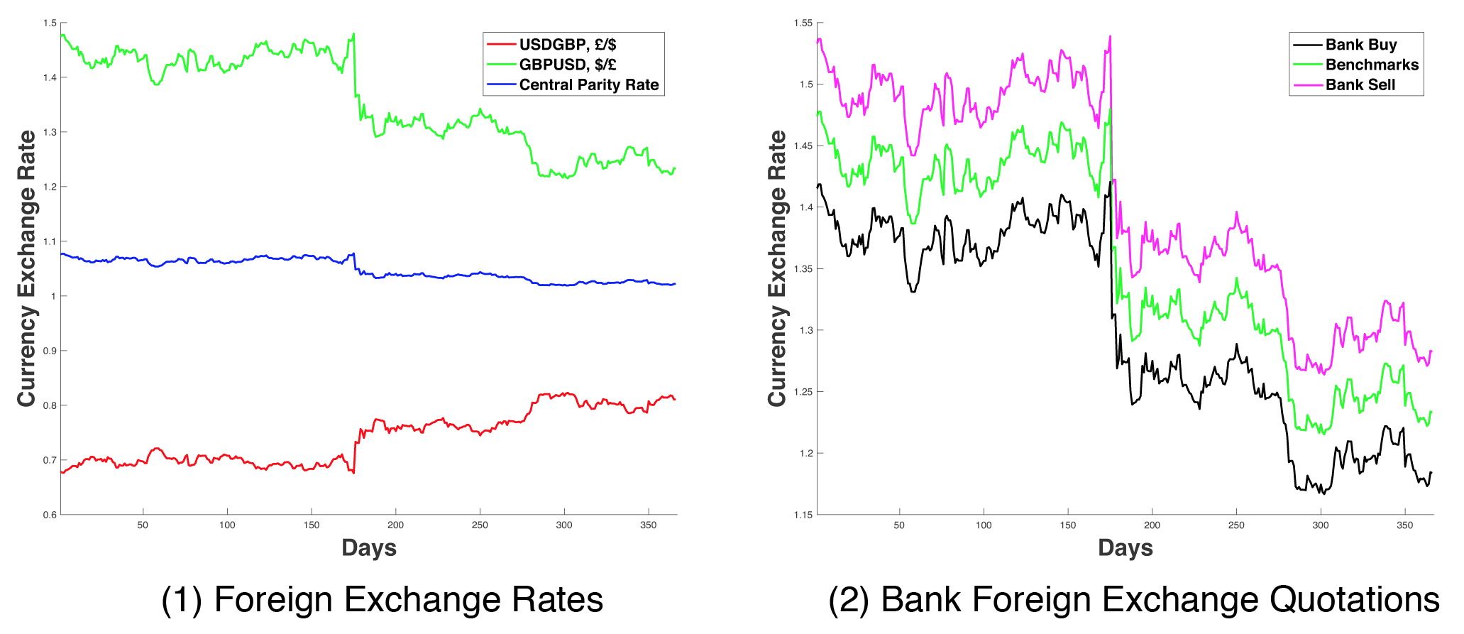
Figure 1: Currecy Exchange Rates

The diagrams below show the currency exchange rates for GBPs against to USDs in 2016. We suppose that the bank is based on UK. In what follows, we shall go into details Figure (1) and Figure (2), one-by-one.

With regard to the Figure (1),

• The horizontal axis is the time parameter from day 1 to day 365 and the vertical axis stands for the currency exchange rates for GBPs and USDs;

• The green line represents the currency exchange rates for GBPs against to USDs, which is the selling price of the USDs for the bank in UK;

• The red line signifies the currency exchange rates for USDs against to GBPs, which is the buying price of the USDs for the bank in UK;

• The blue line means the central parity rates for USDs against to GBPs, which is equal to half of buying price (see green line) plus selling price (see red line).

As the volatility of currency exchange rates, banks also take risks for the price volatility when they sell and buy the currencies. So, each bank adopts different currency exchange rates according to the benchmark rates. Meanwhile, the trader will be charged for each currency transaction.

Concerning the Figure (2),

• The green line is taken from the Figure (1), which is the benchmark rate for the bank. According to the mechanism of foreign exchange markets, banks adjust their own currency exchange rates to hedge the risk from price volatilities. On the other hand, the gap between the pink and the black line is the profit that the bank obtains.

• The pink line is the bank quotation of selling foreign currencies (i.e., USDs), which is greater than the benchmark rate at the same moment.

• The black line stands for the bank quotation of buying foreign currencies (i.e., USDs), which is less than the benchmark rate at the same moment.

As far as the investors are concerned, it is sufficient to look at the pink line (in the Figure (2)) when they buy foreign currencies and watch the black line in the case that they sell foreign currencies. Thus, if an investor buys foreign currencies at one moment, then the profit for the investor depends heavily on the bank quotation of selling foreign currencies exchange rates (see the pink line in the Figure (2)) when the investor sells the currencies bought at the next moment.

As we know, there are numerous factors which have impacts on the currency exchange rates (see e.g. [11] and references therein). Nevertheless, in the present paper, we will not go into details the corresponding influential factors. In this work, we are interested in the prediction of the returns and whether there is an algorithm to optimise the currency portfolios.

2.2 Our foreign exchange market setup

Before we present the set up of the foreign exchange markets, let us introduce some notation and terminology. Let $N>1$ be a fixed integer, which will be called the period of investment in the foreign exchange markets. Throughout the paper, we assume that there are $m~{}(>1)$ different currencies which are tradable in the foreign exchange markets. Set the (ordered) list of currencies by $\Lambda_{0}:=\{1,...,m\}$ and the trading dates by $\Lambda_{1}:=\{1,...,N\}$.

• For each pair $(i,j)\in\Lambda_{0}\times\Lambda_{0}$ with $i<j$, we use $\bar{s}_{ij}^{(k)}$ to denote the currency exchange rate for the investor to buy the foreign currency $j$ via the (home) currency $i$ at the date $k\in\Lambda_{1}$; and for $i>j$, $\underline{s}_{ij}^{(k)}$ stands for the currency exchange rate for the investor to sell the foreign currency $j$ to get the home currency $i$ at the date $k\in\Lambda_{1}$.

• Note that there is a corresponding currency exchange rate for each pair of the $m$ different currencies (indeed, the total number of pairs are $m^{2}$ with $m(m-1)$ distinct pairings). Thus, the currency exchange rates at the date $k$ and the adjacent date $k+1$ can be formed by two square matrices, denoted by $S^{(k)}$ and $S^{(k+1)}$, respectively, as in the following manner

  $$S^{(k)}=\left(\begin{array}[]{ccccc}s_{11}^{(k)}&\bar{s}_{12}^{(k)}&\cdots&\bar{s}_{1m}^{(k)}\\ \underline{s}_{21}^{(k)}&s_{22}^{(k)}&\cdots&\bar{s}_{2m}^{(k)}\\ \vdots&\vdots&\ddots&\vdots\\ \underline{s}_{m1}^{(k)}&\underline{s}_{m2}^{(k)}&\cdots&s_{mm}^{(k)}\\ \end{array}\right)$$ (2.1)

  and

  $$S^{(k+1)}=\left(\begin{array}[]{ccccc}s_{11}^{(k+1)}&\bar{s}_{12}^{(k+1)}&\cdots&\bar{s}_{1m}^{(k+1)}\\ \underline{s}_{21}^{(k+1)}&s_{22}^{(k+1)}&\cdots&\bar{s}_{2m}^{(k+1)}\\ \vdots&\vdots&\ddots&\vdots\\ \underline{s}_{m1}^{(k+1)}&\underline{s}_{m2}^{(k+1)}&\cdots&s_{mm}^{(k+1)}\\ \end{array}\right).$$ (2.2)

• For a square matrix, the entries above the main diagonal are called the upper triangular part and the entries below the main diagonal are named as the lower triangular part. The upper triangular parts and the lower triangular parts of $S^{(k)}$ and $S^{(k+1)}$, defined in (2.1) and (2.2), respectively, are the bank quotations of selling and buying foreign currencies, respectively.

• For $j=i$, $s_{ij}^{(.)}$ means the currency exchange rate of the currency $i$ against to itself at the day $k\in\Lambda_{1}.$ For simplicity, we set $s_{ij}^{(.)}=1$.

• From the point of view for the bank, it is plausible to assume $\bar{s}_{ij}^{(.)}>\underline{s}_{ij}^{(.)}>0$. So, there is a gap between $\bar{s}_{ij}^{(.)}$ and $\underline{s}_{ij}^{(.)}$ so that there exists $\varepsilon>0$ satisfying $\bar{s}_{ij}^{(.)}-\underline{s}_{ij}^{(.)}=2\varepsilon$. Observe that the parameter $\varepsilon$ will be changed according to the transaction amount in the spot market.

• According to the foreign exchange market mechanism (showed in Figure (2)), when trading currencies, investors buy (or sell) foreign currencies at the date $k$ and then sell (or buy) foreign currencies at the day $k+1$. Then we have following two matrices for investors to trade currencies at different time.

  $$S_{(k+1)}^{(k)}=\left(\begin{array}[]{ccccc}s_{11}^{(k)}&\bar{s}_{12}^{(k)}&\cdots&\bar{s}_{1m}^{(k)}\\ \underline{s}_{21}^{(k+1)}&s_{22}^{(k)}&\cdots&\bar{s}_{2m}^{(k)}\\ \vdots&\vdots&\ddots&\vdots\\ \underline{s}_{m1}^{(k+1)}&\underline{s}_{m2}^{(k+1)}&\cdots&s_{mm}^{(k)}\\ \end{array}\right),$$

  and

  $$S_{(k)}^{(k+1)}=\left(\begin{array}[]{ccccc}s_{11}^{(k+1)}&\bar{s}_{12}^{(k+1)}&\cdots&\bar{s}_{1m}^{(k+1)}\\ \underline{s}_{21}^{(k)}&s_{22}^{(k)}&\cdots&\bar{s}_{2m}^{(k+1)}\\ \vdots&\vdots&\ddots&\vdots\\ \underline{s}_{m1}^{(k)}&\underline{s}_{m2}^{(k)}&\cdots&s_{mm}^{(k)}\\ \end{array}\right),$$

  where the lower triangular parts of $S_{(k+1)}^{(k)}$ (resp. $S_{(k)}^{(k+1)}$) are the currency exchange rates for investors to sell (resp. buy ) foreign currencies at the date $k$ (resp. the date $k+1$), and then the upper triangular parts of $S_{(k+1)}^{(k)}$ (resp. $S_{(k)}^{(k+1)}$) are the currency exchange rates for investors to buy foreign currencies at the date $k+1$ (resp. the date $k$).

• Assume that an investor holds the home currency $i$, where the total value is $X_{i}$. At the day $k$, the investor buys the foreign currency $j$, whose value is equal to $X_{i}\bar{s}_{ij}^{(k)}$, via the home currency $i$, then we have the value of foreign currency is $X_{j}(=X_{i}\bar{s}_{ij}^{(k)})$. At the day $k+1$, the investor sells the foreign currency $X_{j}$ to get the home currency $\tilde{X}_{i}$.

• Next, let us define two foreign exchange options $\hat{\bar{s}}_{ij}^{(k+1)}$ and $\hat{\underline{s}}_{ij}^{(k+1)}$ for the currency exchange rates in the date $k+1$, respectively, by

  $$\hat{\bar{s}}_{ij}^{(k+1)}=\begin{cases}\underline{s}_{ij}^{(k+1)},~{}~{}~{}~{}~{}~{}~{}~{}\underline{s}_{ij}^{(k+1)}>\bar{s}_{ij}^{(k)}\\ 0,~{}~{}~{}~{}~{}~{}~{}~{}~{}~{}~{}~{}~{}~{}~{}~{}~{}~{}\mbox{others}\end{cases}$$ (2.3)

  $$\hat{\underline{s}}_{ij}^{(k+1)}=\begin{cases}\underline{s}_{ij}^{(k+1)},~{}~{}~{}~{}~{}~{}~{}~{}\bar{s}_{ij}^{(k+1)}>\underline{s}_{ij}^{(k)}\\ 0,~{}~{}~{}~{}~{}~{}~{}~{}~{}~{}~{}~{}~{}~{}~{}~{}~{}~{}\mbox{others}\end{cases}$$ (2.4)

  That is, there is no investment for investors if it is not profitable.

• For ${(i,j)}^{th}$ currency pair in the market at the date $k$, the return at the date $k$ and the date $k+1$ can be expressed respectively as $\bar{r}_{ij}^{(k)}$, $\underline{r}_{ij}^{(k)}$ and $\bar{r}_{ij}^{(k+1)}$, $\underline{r}_{ij}^{(k+1)}$. Let $\bar{s}_{ij}^{(ko)}$ and $\underline{s}_{ij}^{(ko)}$ be the opening exchange rates at the date $k$, and denote the closing exchange rates of ${(i,j)}^{th}$ currency pair by $\bar{s}_{ij}^{(kc)}$ and $\underline{s}_{ij}^{(kc)}$, then we have the following

  $$\bar{r}_{ij}^{(k)}=\begin{cases}\frac{\bar{s}_{ij}^{(ko)}}{\underline{s}_{ij}^{(kc)}},~{}~{}~{}~{}~{}~{}~{}~{}\bar{s}_{ij}^{(ko)}>\underline{s}_{ij}^{(kc)}\\ 0,~{}~{}~{}~{}~{}~{}~{}~{}~{}~{}~{}~{}~{}~{}~{}~{}~{}~{}\mbox{others};\end{cases}\quad\bar{r}_{ij}^{(k+1)}=\begin{cases}\frac{\bar{s}_{ij}^{(ko)}}{\underline{s}_{ij}^{(k+1)c}},~{}~{}~{}~{}~{}~{}~{}~{}\bar{s}_{ij}^{(ko)}>\underline{s}_{ij}^{(k+1)c}\\ 0,~{}~{}~{}~{}~{}~{}~{}~{}~{}~{}~{}~{}~{}~{}~{}~{}~{}~{}\mbox{others}\end{cases}$$ (2.5)

  and

  $$\underline{r}_{ij}^{(k)}=\begin{cases}\frac{\underline{s}_{ij}^{(ko)}}{\bar{s}_{ij}^{(kc)}},~{}~{}~{}~{}~{}~{}~{}~{}\underline{s}_{ij}^{(ko)}>\bar{s}_{ij}^{(kc)}\,\\ 0,~{}~{}~{}~{}~{}~{}~{}~{}~{}~{}~{}~{}~{}~{}~{}~{}~{}~{}\mbox{others};\end{cases}\quad\underline{r}_{ij}^{(k+1)}=\begin{cases}\frac{\underline{s}_{ij}^{(ko)}}{\bar{s}_{ij}^{(k+1)c}},~{}~{}~{}~{}~{}~{}~{}~{}\underline{s}_{ij}^{(ko)}>\bar{s}_{ij}^{(k+1)c}\\ 0,~{}~{}~{}~{}~{}~{}~{}~{}~{}~{}~{}~{}~{}~{}~{}~{}~{}~{}\mbox{others}.\end{cases}$$ (2.6)

• The return matrices $R^{(k)}$ and $R^{(k+1)}$ of the $m$ currency exchange transactions at the trading dates $k$ and $k+1$ are defined respectively by

  $$R^{(k)}=\left(\begin{array}[]{ccccc}r_{11}^{(k)}&\bar{r}_{12}^{(k)}&\cdots&\bar{r}_{1m}^{(k)}\\ \underline{r}_{21}^{(k)}&r_{22}^{(k)}&\cdots&\bar{r}_{2m}^{(k)}\\ \vdots&\vdots&\ddots&\vdots\\ \underline{r}_{m1}^{(k)}&\underline{r}_{m2}^{(k)}&\cdots&r_{mm}^{(k)}\\ \end{array}\right)$$ (2.7)

  and

  $$R^{(k+1)}=\left(\begin{array}[]{ccccc}r_{11}^{(k)}&\bar{r}_{12}^{(k+1)}&\cdots&\bar{r}_{1m}^{(k+1)}\\ \underline{r}_{21}^{(k+1)}&r_{22}^{(k)}&\cdots&\bar{r}_{2m}^{(k+1)}\\ \vdots&\vdots&\ddots&\vdots\\ \underline{r}_{m1}^{(k+1)}&\underline{r}_{m2}^{(k+1)}&\cdots&r_{mm}^{(k+1)}\\ \end{array}\right).$$ (2.8)

  Note that $\bar{r}_{ij}^{(.)}\neq 0$ whenever $\underline{r}_{ji}^{(.)}=0$ and reciprocally $\underline{r}_{ij}^{(.)}\neq 0$ whenever $\bar{r}_{ji}^{(.)}=0$. Moreover, $r_{ji}^{(.)}=0$ for $i=j$. In literature, the return matrix $R^{(k)}$ is also referred to as a price relative, see, for instance, [1].

• For each pair $(i,j)$ of the $m$ different currencies, let $\psi_{ij}^{(k)}$ denote the proportion of the whole capital the investor holds at the date $k$ to buy the foreign currency $j$ via the home currency $i$. Then, the portfolio matrix $\psi^{(k)}$ for the $m$ different currencies at the date $k$ can be formulated as

  $$\psi^{(k)}=\left(\begin{array}[]{ccccc}\psi_{11}^{(k)}&\psi_{12}^{(k)}&\cdots&\psi_{1m}^{(k)}\\ \psi_{21}^{(k)}&\psi_{22}^{(k)}&\cdots&\psi_{2m}^{(k)}\\ \vdots&\vdots&\ddots&\vdots\\ \psi_{m1}^{(k)}&\psi_{m2}^{(k)}&\cdots&\psi_{mm}^{(k)}\\ \end{array}\right).$$ (2.9)

  Note that, for $i,j\in\Lambda_{0}$, $\psi_{ij}^{(k)}\geq 0,\psi_{ii}^{(k)}=0,\sum_{i,j=1}^{m}\psi_{ij}^{(k)}=1$. In what follows, let $P^{(k)}$ be the collection of all portfolio matrices for the $m$ different currencies at the date $k$, i.e.,

  $$P^{(k)}:=\Big{\{}\psi^{(k)}\in\mathbb{R}^{m}\otimes\mathbb{R}^{m}:\sum_{i,j\in\Lambda_{0}}\psi_{ij}^{(k)}=1,\psi_{ij}^{(k)}>0,\psi_{ii}^{(k)}=0,i,j\in\Lambda_{0}\Big{\}},$$

  where $\mathbb{R}^{m}\otimes\mathbb{R}^{m}$ stands for the totality of $m\times m$-matrices.

• For $A=(a_{ij})_{m\times m}\,,B=(b_{ij})_{m\times m}\in\mathbb{R}^{m}\otimes\mathbb{R}^{m}$, we define a product by the following

  $$A\boxtimes B:=(c_{ij})_{m\times m}\in\mathbb{R}^{m}\otimes\mathbb{R}^{m},$$ (2.10)

  in which $c_{ij}:=a_{ij}b_{ij}.$

• The return matrix $\psi^{(k)}\boxtimes R^{(k)}$ of the portfolio matrix $\psi^{(k)}$ is given by

  $$\psi^{(k)}\boxtimes R^{(k)}=\left(\begin{array}[]{ccccc}0&\psi_{12}^{(k)}\bar{r}_{12}^{(k)}&\cdots&\psi_{1m}^{(k)}\bar{r}_{1m}^{(k)}\\ \psi_{21}^{(k)}\underline{r}_{21}^{(k)}&0&\cdots&\psi_{2m}^{(k)}\bar{r}_{2m}^{(k)}\\ \vdots&\vdots&\ddots&\vdots\\ \psi_{m1}^{(k)}\underline{r}_{m1}^{(k)}&\psi_{m2}^{(k)}\underline{r}_{m2}^{(k)}&\cdots&0\\ \end{array}\right)$$

  according to (2.10).

• Let $F_{k}$ be the capital the investor holds at the end of the date $k$ and $T_{k}$ the transaction costs charged at the day $k$. We assume that the capital at the end of the date $k$ is same as the begginning of the day $k+1$. Let $F^{\prime}_{k}$ be the total funds at the date $k$ whenever the transaction costs are taken into consideration. Obviously,

  $$F^{\prime}_{k}=F_{k-1}-T_{k},\quad k\geqslant 1.$$ (2.11)

• Set

  $$\psi^{(k)}\diamond R^{(k)}:=\left(\begin{array}[]{ccccc}1&1&\cdots&1\\ \end{array}\right)_{(1\times m)}\Big{(}\psi^{(k)}\boxtimes R^{(k)}\Big{)}\left(\begin{array}[]{c}1\\ 1\\ \vdots\\ 1\\ \end{array}\right)_{(m\times 1)}.$$

  Thus, it is obvious to see that the scalar value

  $$\psi^{(k)}\diamond R^{(k)}=\sum_{i,j=1}^{m}\Big{(}\psi_{ij}^{(k)}\Big{(}\bar{r}^{(k)}_{ij}+\underline{r}^{(k)}_{ij}\Big{)}\Big{)}$$ (2.12)

  and, by taking the transaction costs into account, we have

  $$F_{k}=F^{\prime}_{k}(\psi^{(k)}\diamond R^{(k)}).$$ (2.13)

2.3 The on-line portfolio strategy

As the high volatility of the currency exchange rates, the investor prefers to adjust the investment strategy frequently. It is worthwhile pointing out that one of the effective strategy to optimize the portfolio matrix is the on-line portfolio selection by taking advantage of the historical data. More precisely,

• The on-line portfolio strategy is given by

  $$\psi^{(k+1)}=f\Big{(}\{\psi^{(1)},...,\psi^{(k)}\},\{R^{(1)},...,R^{(k)}\}\Big{)},$$

  where $f:(\mathbb{R}^{m}\otimes\mathbb{R}^{m})^{2k}\rightarrow P^{(k+1)}$ with

  $$(\mathbb{R}^{m}\otimes\mathbb{R}^{m})^{2k}:=\underbrace{\mathbb{R}^{m}\otimes\mathbb{R}^{m}\cdots\times\mathbb{R}^{m}\otimes\mathbb{R}^{m}}_{2k}.$$

  It is clear to see that the on-line portfolio strategy $\psi^{(k+1)}$ depends on the portfolio matrices and the return matrices before the $(k+1)$-th trading date.

• Without taking the transaction costs into consideration, the total capital during the course of the investment period (i.e., $N$ days) will increase to

  $$I_{N}\Big{(}\{\psi^{(\cdot)}\},\{R^{(\cdot)}\}\Big{)}:=\prod_{k=1}^{N}\bigg{\{}\psi^{(k)}\diamond R^{(k)}\bigg{\}},$$ (2.14)

  where $\psi^{(k)}\diamond R^{(k)}$ is given in (2.12). Herein, $I_{N}\Big{(}\{\psi^{(\cdot)}\},\{R^{(\cdot)}\}\Big{)}$ is referred to as the final return without the transaction costs. With (2.14) in hand, the exponential growth rate of the funds without the transaction costs is represented by

  $$LI_{N}(\{\psi^{(\cdot)}\},\{R^{(\cdot)}\}):=\frac{1}{N}\sum_{k=1}^{N}\log\bigg{(}\psi^{(k)}\diamond R^{(k)}\bigg{)}.$$ (2.15)

• Let $(c_{k})_{k\in\Lambda_{1}}$ with $c_{1}=0$ be the ratio of the transaction cost at the date $k$ (i.e., $T_{k}$) to the fund holding at the beginning of the date $k$ (i.e., $F_{k-1}$), in other words,

  $$c_{1}=0;\qquad c_{k}=\frac{T_{k}}{F_{k-1}}=\frac{F_{k-1}-F^{\prime}_{k}}{F_{k-1}},~{}~{}~{}~{}~{}k\geq 2,$$ (2.16)

  where the second identity for $c_{k}$ is due to (2.11) and $F_{k}>0$ for $k\geq 1.$

• In the presence of the transaction costs, the return of the total investment during the investment period will reach to

  $$F_{N}(\{\psi^{(\cdot)}\},\{R^{(\cdot)}\})=\prod_{k=1}^{N}\Big{(}\psi^{(k)}\diamond R^{(k)}\Big{)}(1-c_{k}),$$ (2.17)

  where $c_{k}$ is defined as in (2.16). In (2.17), $F_{N}(\{\psi^{(\cdot)}\},\{R^{(\cdot)}\})$ is named as the return with the transaction costs. With the (2.17), we formulate the exponential growth rate of the funds with transaction costs as

  $$R_{N}(\{\psi^{(\cdot)}\},\{R^{(\cdot)}\}):=\frac{1}{N}\sum_{k=1}^{N}\log\bigg{(}\psi^{(k)}\diamond R^{(k)}\bigg{)}+\frac{1}{N}\sum_{k=1}^{N}\log(1-c_{k}).$$ (2.18)

2.4 Transaction costs

According to the self-financing strategy, the investor will reinvest all of the funds held at the end of the trading date $k-1,\mbox{for }k\geq 2$ to the beginning of the next trading date $k$. In our present case, we shall consider the transaction costs at the end of the trading date. Hence, the total funds will be reduced. For more details, the reader is referred to (2.11). In the light of (2.13), the investment on the currency pair $(i,j)$ admits the form

$$X^{k}_{ij}=F^{\prime}_{k}\psi^{(k)}_{ij}\Big{(}\bar{r}^{(k)}_{ij}+\underline{r}^{(k)}_{ij}\Big{)},$$ (2.19)

where $F^{\prime}_{k}$ is introduced in (2.11). At the trading date $k+1$, the investor will hold a new portfolio matrix $\psi^{(k+1)}$. Meanwhile, at the date $k+1,$ the transaction cost $T_{k+1}$ will be charged by the bank involved so that the funds at the date $k+1$ is $F^{\prime}_{k+1}=F_{k}-T_{k+1}$. Thus, the investment for the currency pair $(i,j)$ at the date $k+1$ is

$$X^{\prime(k+1)}_{ij}=F^{\prime}_{k+1}\psi^{(k+1)}_{ij}.$$ (2.20)

Henceforth, from (2.19) and (2.20), it follows that the transaction cost between the currency pair $(i,j)$ is

$$|X^{\prime(k+1)}_{ij}-X^{k}_{ij}|=\Big{|}F^{\prime}_{k+1}\psi^{(k+1)}_{ij}-F^{\prime}_{k}\psi^{(k)}_{ij}\Big{(}\bar{r}^{(k)}_{ij}+\underline{r}^{(k)}_{ij}\Big{)}\Big{|}.$$ (2.21)

We further suppose (for simplicity) that the transaction costs are the same for selling and buying foreign currencies. As a consequence, (2.11) and (2.21) imply that the total transaction costs at the start of the date $(k+1)$ is

$$\begin{split}Q_{k+1}=\sum_{i,j=1}^{m}|X^{\prime(k+1)}_{ij}-X^{k}_{ij}|&=\sum_{i,j=1}^{m}\Big{|}F^{\prime}_{k+1}\psi^{(k+1)}_{ij}-F^{\prime}_{k}\psi^{(k)}_{ij}\Big{(}\bar{r}^{(k)}_{ij}+\underline{r}^{(k)}_{ij}\Big{)}\Big{|}\\ &=\sum_{i,j=1}^{m}\Big{|}(F_{k}-T_{k+1})\psi^{(k+1)}_{ij}-F^{\prime}_{k}\psi^{(k)}_{ij}\Big{(}\bar{r}^{(k)}_{ij}+\underline{r}^{(k)}_{ij}\Big{)}\Big{|}.\end{split}$$ (2.22)

In the case that the transaction costs $T_{k+1}$ is linearly dependent on the total investment $Q_{k+1}$ in the trading date $k+1$, there exists a positive constant $c$ such that $T_{k+1}=cQ_{k+1}$. Accordingly, (2.22) yields that

$$T_{k+1}=cQ_{k+1}=\sum_{i,j=1}^{m}\Big{|}F_{k}\psi^{(k+1)}_{ij}-F^{\prime}_{k}\psi^{(k)}_{ij}\Big{(}\bar{r}^{(k)}_{ij}+\underline{r}^{(k)}_{ij}\Big{)}-T_{k+1}\psi^{(k+1)}_{ij}\Big{|}.$$ (2.23)

For $\psi^{(k+1)}\in P^{(k+1)}$ and $T_{k+1}\geqslant 0$, we set

$$\Delta_{k+1}:=\sum_{i,j=1}^{m}\Big{|}F_{k}\psi^{(k+1)}_{ij}-F^{\prime}_{k}\psi^{(k)}_{ij}\Big{(}\bar{r}^{(k)}_{ij}+\underline{r}^{(k)}_{ij}\Big{)}\Big{|}.$$

It is easy to see that

$$c\Big{(}\Delta_{k+1}-\sum_{i,j=1}^{m}T_{k+1}\psi^{(k+1)}_{ij}\Big{)}\leq T_{k+1}\leq c\Big{(}\Delta_{k+1}+\sum_{i,j=1}^{m}T_{k+1}\psi^{(k+1)}_{ij}\Big{)}.$$

This, together with $\psi^{(k+1)}\in P^{(k+1)}$ and $\sum_{i,j=1}^{m}\psi^{(k+1)}_{ij}=1$, leads to

$$c\Big{(}\Delta_{k+1}-T_{k+1}\Big{)}\leq T_{k+1}\leq c\Big{(}\Delta_{k+1}+\ T_{k+1}\Big{)}.$$ (2.24)

If $c<1$, then, we derive from (2.24) that

$$\frac{c}{1+c}\Delta_{k+1}\leqslant T_{k+1}\leqslant\frac{c}{1-c}\Delta_{k+1}.$$ (2.25)

Let

$${\psi^{\prime}}^{(k)}:=\left(\begin{array}[]{ccccc}{\psi^{\prime}}_{11}^{(k)}&{\psi^{\prime}}_{12}^{(k)}&\cdots&{\psi^{\prime}}_{1m}^{(k)}\\ {\psi^{\prime}}_{21}^{(k)}&{\psi^{\prime}}_{22}^{(k)}&\cdots&{\psi^{\prime}}_{2m}^{(k)}\\ \vdots&\vdots&\ddots&\vdots\\ {\psi^{\prime}}_{m1}^{(k)}&{\psi^{\prime}}_{m2}^{(k)}&\cdots&{\psi^{\prime}}_{mm}^{(k)}\\ \end{array}\right),$$

with

$${\psi^{\prime}}^{(k)}_{ij}:=\frac{F^{\prime}_{k}}{F_{k}}\psi^{(k)}_{ij}\Big{(}\bar{r}^{(k)}_{ij}+\underline{r}^{(k)}_{ij}\Big{)}.$$ (2.26)

We remark that ${\psi^{\prime}}^{(k)}$ is the proportion matrix for the $m$ different currencies reached automatically at the end of the date $k$.

In what follows, we assume that $F_{k}>0$ and $\psi^{(k)}\diamond R^{(k)}>0.$ We define the distance between $\psi^{(k+1)}$ and $\psi^{\prime(k)}$ by

$$d(\psi^{(k+1)},\psi^{\prime k}):=\sum_{i,j=1}^{m}|\psi^{(k+1)}_{ij}-\psi^{\prime(k)}_{ij}|.$$ (2.27)

By virtue of the notion of $\Delta_{k+1}$, one has

$$\begin{split}\Delta_{k+1}=F_{k}\sum_{i,j=1}^{m}\Big{|}\psi^{(k+1)}_{ij}-\frac{F^{\prime}_{k}}{F_{k}}\psi^{(k)}_{ij}\Big{(}\bar{r}^{(k)}_{ij}+\underline{r}^{(k)}_{ij}\Big{)}\Big{)}\Big{|}.\end{split}$$

This, combining with (2.26), gives that

$$\Delta_{k+1}=F_{k}\sum_{i,j=1}^{m}\Big{|}\psi^{(k+1)}_{ij}-{\psi^{\prime}}^{(k)}_{ij}\Big{|}=F_{k}d(\psi^{(k+1)},\psi^{\prime(k)}).$$

Substituting this into (2.25), we end up with the following

$$\frac{c}{1+c}F_{k}d(\psi^{(k+1)},\psi^{\prime(k)})\leqslant T_{k+1}\leqslant\frac{c}{1-c}F_{k}d(\psi^{(k+1)},\psi^{\prime(k)}).$$ (2.28)

From (2.28), we observe that the transaction cost at the date $k+1$ depends on the distance between $\psi^{(k+1)}$ and $\psi^{\prime(k)}$, and that the bigger distance between $\psi^{(k+1)}$ and $\psi^{\prime(k)}$ means the more transaction costs which further implies less profit in the portfolio. Hence, to improve the profit for the portfolios, it is essential for the investors to shorten the distance between $\psi^{(k+1)}$ and $\psi^{\prime(k)}$ .

3 Update rules for on-line portfolio selections

As the high volatility of the currency exchange rates, the investors, in general, try to buy and sell the currencies again and again to get more profits. Unfortunately, the more transactions means the more transaction costs. So, it is indispensable to optimise the portfolios in order to evade the unnecessary transaction costs, which is our goal in this section.

Let $Z(\psi^{(k+1)})$ be the return of the portfolio $\psi^{(k+1)}$ at the date $k+1$ and assume that $Z(\cdot)$ admits the following form

$$Z(\psi^{(k+1)})=\gamma Z_{F}(\psi^{(k+1)},R^{\prime(k+1)})-Z_{T}(\psi^{(k+1)}),$$ (3.1)

where

• $$R^{\prime(k+1)}:=\left(\begin{array}[]{ccccc}r_{11}^{{}^{\prime}(k+1)}&\bar{r}_{12}^{{}^{\prime}(k+1)}&\cdots&\bar{r}_{1m}^{{}^{\prime}(k+1)}\\ \underline{r}_{21}^{{}^{\prime}(k+1)}&r_{22}^{{}^{\prime}(k+1)}&\cdots&\bar{r}_{2m}^{{}^{\prime}(k+1)}\\ \vdots&\vdots&\ddots&\vdots\\ \underline{r}_{m1}^{{}^{\prime}(k+1)}&\underline{r}_{m2}^{{}^{\prime}(k+1)}&\cdots&r_{mm}^{{}^{\prime}(k+1)}\\ \end{array}\right)$$ (3.2)

  is the prediction of return matrix $R^{(k+1)}$ at the date $k+1;$

• $Z_{F}(\psi^{(k+1)},R^{\prime(k+1)})$ is a function of investment increments with respect to the portfolio matrix $\psi^{(k+1)}$ and the prediction $R^{\prime(k+1)}$ of $R^{(k+1)}$;

• $Z_{T}(\psi^{(k+1)})$ is the transaction cost which the investor pays for the portfolio matrix $\psi^{(k+1)}$;

• $\gamma>0$ is a parameter adopted to balance maximizing the investment increase and reducing the transactions.

In the present paper, the first alternative for the function $Z_{F}$, denoted by $Z_{F}^{(1)}$, admits the form

$$Z_{F}^{(1)}(\psi^{(k+1)},R^{\prime(k+1)})=\psi^{(k+1)}\diamond R^{\prime(k+1)}.$$ (3.3)

And the second choice for $Z_{F}$, written by $Z_{F}^{(2)}$, possesses the following representation

$$\begin{split}Z_{F}^{(2)}\Big{(}\psi^{(k+1)},R^{\prime(k+1)}\Big{)}=\log\Big{(}\psi^{\prime(k)}\diamond R^{\prime(k+1)}\Big{)}+\frac{R^{\prime(k+1)}\Big{(}\psi^{(k+1)}-\psi^{\prime(k)}\Big{)}}{\psi^{(k+1)}\diamond R^{\prime(k+1)}}.\end{split}$$ (3.4)

By the Taylor expansion formula for the multivariate functions, we deduce that

$$\begin{split}\log(\psi^{(k+1)}\diamond R^{\prime(k+1)})&\approx\log\bigg{(}\sum_{i,j=1}^{m}\Big{(}{\psi^{\prime}}_{ij}^{(k)}(\bar{r}_{ij}^{{}^{\prime}(k+1)}+\underline{r}_{ij}^{{}^{\prime}(k+1)})\Big{)}\bigg{)}\\ &\quad+\frac{\sum_{i,j=1}^{m}(\bar{r}_{ij}^{{}^{\prime}(k+1)}+\underline{r}_{ij}^{{}^{\prime}(k+1)})\Big{(}\psi_{ij}^{(k+1)}-\psi_{ij}^{\prime(k)}\Big{)}}{\sum_{i,j=1}^{m}\psi_{ij}^{(k+1)}(\bar{r}_{ij}^{{}^{\prime}(k+1)}+\underline{r}_{ij}^{{}^{\prime}(k+1)})}.\end{split}$$

Therefore, $Z_{F}^{(2)}\Big{(}\psi^{(k+1)},R^{\prime(k+1)}\Big{)}$ is the first order approximation of $\log(\psi^{(k+1)}\diamond R^{\prime(k+1)})$.

With regard to the term $Z_{T}(\psi^{(k+1)})$, we define

$$Z_{T}(\psi^{(k+1)}):=d_{\mbox{re}}\Big{(}\psi^{(k+1)},\psi^{\prime(k)}\Big{)}.$$ (3.5)

We refer the reader to [1, 8, 9] for more details. According to the definition of relative entropy for discrete random variables, we have the following

$$\begin{split}d_{\mbox{re}}\Big{(}\psi^{(k+1)},\psi^{\prime(k)}\Big{)}&=\sum_{i,j=1}^{m}\bigg{(}\psi^{(k+1)}_{ij}\log\frac{\psi^{(k+1)}_{ij}}{\psi^{\prime(k)}_{ij}}\bigg{)}\\ &=\sum_{i,j=1}^{m}\bigg{(}\psi^{(k+1)}_{ij}\log\frac{\psi^{(k+1)}_{ij}\sum_{i,j=1}^{m}\Big{(}\psi_{ij}^{(k)}(\bar{r}^{(k)}_{ij}+\underline{r}^{(k)}_{ij})\Big{)}}{\psi^{(k)}_{ij}(\bar{r}^{(k)}_{ij}+\underline{r}^{(k)}_{ij})}\bigg{)}.\end{split}$$ (3.6)

By L’Hospital’s rule, one has $\lim_{x\downarrow 0}x\log x=0$. So, without loss of generality, in (3.6), we can assume $\psi^{(k+1)}_{ij}\log\psi^{(k+1)}_{ij}=0$ whenever $\psi^{(k+1)}_{ij}=0.$ Note that for any constant $a>1,f(x)=x(\log x+\log a)$ is a convex function for $x>0$ due to the fact that $f^{\prime\prime}(x)>0$. Therefore, $d_{\mbox{re}}\Big{(}\psi^{(k+1)},\psi^{\prime(k)}\Big{)}$ is a positive continuous convex function of $\psi^{(k+1)}_{ij},1\leq i,j\leq m$. If $\psi^{(k+1)}=\psi^{\prime(k)}$, i.e., $\psi^{(k+1)}_{ij}=\psi^{\prime(k)}_{ij}$, then $d_{\mbox{re}}\Big{(}\psi^{(k+1)},\psi^{\prime(k)}\Big{)}=0$. The minimum of $d_{\mbox{re}}\Big{(}\psi^{(k+1)},\psi^{\prime(k)}\Big{)}$ can be achieved at $\psi^{(k+1)}=\psi^{\prime(k)}$. Moreover, let $i_{0},j_{0}\geq 1$ be such that $\psi^{\prime(k)}_{i_{0}j_{0}}=\min\{\psi^{\prime(k)}_{ij}\}$. Then the maximum of $d_{\mbox{re}}\Big{(}\psi^{(k+1)},\psi^{\prime(k)}\Big{)}$ can be available whenever $\psi^{(k+1)}_{ij}=1$ for $i=i_{0},j=j_{0}$, otherwise $\psi^{(k+1)}_{ij}=0$. Inserting (3.3), (3.4) and (3.5) back into (3.1), respectively, we arrive at

$$Z^{\prime(1)}(\psi^{(k+1)})=\gamma\Big{(}\psi^{k+1}\diamond R^{\prime(k+1)}\Big{)}-\sum_{i,j=1}^{m}\bigg{(}\psi^{(k+1)}_{ij}\log\frac{\psi^{(k+1)}_{ij}}{\psi^{\prime(k)}_{ij}}\bigg{)}$$ (3.7)

and

$$\begin{split}Z^{\prime(2)}(\psi^{(k+1)})&=\gamma\log\Big{(}\psi^{\prime(k)}\diamond R^{\prime(k+1)}\Big{)}+\frac{R^{\prime(k+1)}\Big{(}\psi^{(k+1)}-\psi^{\prime(k)}\Big{)}}{\psi^{(k+1)}\diamond R^{\prime(k+1)}}\\ &\quad-\sum_{i,j=1}^{m}\bigg{(}\psi^{(k+1)}_{ij}\log\frac{\psi^{(k+1)}_{ij}}{\psi^{\prime(k)}_{ij}}\bigg{)}.\end{split}$$ (3.8)

As $d_{\mbox{re}}$ is convex (as shown above) with respect to $\psi^{(k+1)}_{ij}$, $-d_{\mbox{re}}$ is concave with respect to $\psi^{(k+1)}_{ij}$. Observe that, except the entropy term $d_{\mbox{re}}$, the other terms are linear with respect to $\psi^{(k+1)}_{ij}$, which are obviously concave. As a result, we conclude that $Z^{\prime(1)}(\psi^{(k+1)})$ and $Z^{\prime(2)}(\psi^{(k+1)})$, defined in (3.7) and (3.8), respectively, are concave functions with respect to the portfolio matrix entries $\psi^{(k+1)}_{ij}$.

To maximise $Z^{\prime(1)}(\psi^{(k+1)})$ with the constraint $\psi^{(k+1)}\in P^{(k+1)}$ (so that $\sum_{i,j=1}^{m}\psi^{(k+1)}_{ij}=1$), we utilise Lagrange’s method. To this end, we consider the following auxiliary function

$$\begin{split}Z^{\prime(1)}(\psi^{(k+1)},\lambda)&=Z^{\prime(1)}(\psi^{(k+1)})+\lambda\Big{(}\sum_{i,j=1}^{m}\psi^{(k+1)}_{ij}-1\Big{)}\end{split}$$

where $\lambda\in R$ is the Lagrange multiplier. According to (2.12) and (3.7), we obtain that

$$\begin{split}Z^{\prime(1)}(\psi^{(k+1)},\lambda)&=\gamma\sum_{i,j=1}^{m}\psi^{(k+1)}_{ij}\Big{(}\bar{r}_{ij}^{{}^{\prime}(k+1)}+\underline{r}_{ij}^{{}^{\prime}(k+1)}\Big{)}-\sum_{i,j=1}^{m}\bigg{(}\psi^{(k+1)}_{ij}\log\frac{\psi^{(k+1)}_{ij}}{\psi^{\prime(k)}_{ij}}\bigg{)}\\ &\quad+\lambda\Big{(}\sum_{i,j=1}^{m}\psi^{(k+1)}_{ij}-1\Big{)}.\end{split}$$ (3.9)

Taking derivatives with respect to the variables $\psi^{(k+1)}_{ij}$ and $\lambda$ for $Z^{\prime(1)}(\psi^{(k+1)},\lambda)$ followed by letting $\frac{\partial}{\partial\psi^{(k+1)}_{ij}}Z^{\prime(1)}(\psi^{(k+1)},\lambda)=\frac{\partial}{\partial\lambda}Z^{\prime(1)}(\psi^{(k+1)},\lambda)=0$, we then have

$$\begin{split}\gamma\Big{(}\bar{r}_{ij}^{{}^{\prime}(k+1)}+\underline{r}_{ij}^{{}^{\prime}(k+1)}\Big{)}-\log\psi^{(k+1)}_{ij}+\log\psi^{\prime(k)}_{ij}-1+\lambda=0.\end{split}$$

This further implies that

$$\begin{split}\psi^{(k+1)}_{ij}&=\exp\bigg{(}\gamma\Big{(}\bar{r}_{ij}^{{}^{\prime}(k+1)}+\underline{r}_{ij}^{{}^{\prime}(k+1)}\Big{)}+\log\psi^{\prime(k)}_{ij}-1+\lambda\bigg{)}\\ &=\frac{\psi^{\prime(k)}_{ij}\exp\bigg{(}\gamma\Big{(}\bar{r}_{ij}^{{}^{\prime}(k+1)}+\underline{r}_{ij}^{{}^{\prime}(k+1)}\Big{)}\bigg{)}}{\text{\rm{e}}^{1-\lambda}}.\end{split}$$ (3.10)

In view of $\sum_{i,j=1}^{m}\psi^{(k+1)}_{ij}=1$, we get from (3.10) that

$$\sum_{l,v=1}^{m}\frac{\psi^{\prime(k)}_{lv}\exp\bigg{(}\gamma\Big{(}\bar{r}_{lv}^{{}^{\prime}(k+1)}+\underline{r}_{lv}^{{}^{\prime}(k+1)}\Big{)}\bigg{)}}{\text{\rm{e}}^{1-\lambda}}=1.$$

Therefore, it follows that

$$\text{\rm{e}}^{1-\lambda}=\sum_{l,v=1}^{m}\psi^{\prime(k)}_{lv}\exp\bigg{(}\gamma\Big{(}\bar{r}_{lv}^{{}^{\prime}(k+1)}+\underline{r}_{lv}^{{}^{\prime}(k+1)}\Big{)}\bigg{)}.$$

Substituting this into (3.10) leads to

$$\psi^{(k+1)}_{ij}=\frac{\psi^{\prime(k)}_{ij}\exp(\gamma(\bar{r}_{ij}^{{}^{\prime}(k+1)}+\underline{r}_{ij}^{{}^{\prime}(k+1)}))}{\sum_{v,l=1}^{m}\psi^{\prime(k)}_{vl}\exp(\gamma(\bar{r}_{vl}^{{}^{\prime}(k+1)}+\underline{r}_{vl}^{{}^{\prime}(k+1)}))}.$$ (3.11)

(3.11) is the update rule of the Increment of the Investment with Transaction Cost (IITC for abbreviation) for the $(k+1)^{th}$ trading day.

Mimicking the procedure for the derivation of (3.11), one can conclude that $Z^{\prime(2)}(\psi^{(k+1)})$ reaches its maximum at

$$\psi^{(k+1)}_{ij}=\frac{\psi^{\prime(k)}_{ij}\exp\Big{(}\frac{\gamma(\bar{r}_{ij}^{{}^{\prime}(k+1)}+\underline{r}_{ij}^{{}^{\prime}(k+1)})}{\psi^{\prime(k)}\diamond R^{\prime(k+1)}}\Big{)}}{\sum_{v,l=1}^{m}\psi^{\prime(k)}_{vl}\exp\Big{(}\frac{\gamma(\bar{r}_{vl}^{{}^{\prime}(k+1)}+\underline{r}_{vl}^{{}^{\prime}(k+1)})}{\psi^{\prime(k)}\diamond R^{\prime(k+1)}}\Big{)}}.$$ (3.12)

In our case, (3.12) is the update rule of the Exponential Increment of the Investment with Transaction Cost (EIITC for short) for the trading day $k+1$.

It is clear to see that, in (3.11) and (3.12), there are two parameters $\gamma$ and $R^{\prime(k+1)}$ to be selected for the portfolio matrix $\psi^{(k+1)}$. Concerning the variable $\gamma$, different values yield different strategies. We would like to explicate a bit more details about the implications of the parameter $\gamma$. More precisely, (i) $\gamma$ stands for the passive strategy; (ii) the smaller $\gamma$ signifies a weaker prediction of the portfolio matrix $\psi^{(k+1)}$ so that the investors prefer to hold the present portfolio matrix (i.e.,$\psi^{(k)}$) to avoid the decrements; (iii) the bigger $\gamma$ represents a stronger prediction of the portfolio matrix $\psi^{(k+1)}$ so as to the investors prefer to change the present portfolio matrix (i.e., $\psi^{(k)}$) to earn more profits. With regard to $R^{\prime(k+1)}$, it is the prediction of the return at date $k+1$. Clearly, a high quality prediction is a power tool for investors to make a profitable decision for their investments.

Before ending up this section, let us give some remarks.

Remark 3.1

The quantity $Z_{F}^{(1)}(\psi^{(k+1)},R^{\prime(k+1)})$ indicates the increment of the fund at the date $k+1$. On the other hand, one can apply the distance of portfolio matrices $\psi^{\prime(k)}$ and $\psi^{(k+1)}$, defined in (2.27), to measure the decrement function.

Remark 3.2

Apparently, in the realistic financial market, the investors prefer to give up the unprofitable transactions and to add profitable ones instead, in order to avoid the decrements. Consequently, the update rules (3.11) and (3.12) can be attainable.

4 Prediction of the returns

Prediction of the returns for a portfolio plays a vital role in optimising the portfolios in the foreign exchange markets. Motivated by [1], in this paper, we shall establish an algorithm to keep and/or to inject profitable pairs of currencies and to remove unprofitable pairs, which will be called the cross rate algorithm.

In terms of the mechanism of the foreign exchange market, some entries in the return matrix are vanished, see Equations (2.3) - (2.6). More precisely, for any $(i,j)\in\Lambda_{0}\times\Lambda_{0}$, $\bar{r}_{ij}^{(k)}=0$ whenever $\underline{r}_{ij}^{(k)}\neq 0$, while $\bar{r}_{ij}^{(k)}\neq 0$ for $\underline{r}_{ij}^{(k)}=0$, and moreover $r_{ii}^{(k)}=0$. Therefore, there are $\frac{m(m-1)}{2}$ non-zero components in the return matrix. As it is known, in the foreign currency market, the best profitable pair of currencies means the value of the return in the return matrix reaches to the maximum. In the sequel, let $R^{(k)}$ be the return matrix of the $m$ different currencies. Let $\alpha:=\max\{\bar{r}_{ij}^{(k)},\underline{r}_{ij}^{(k)},\,i,j\in\Lambda_{0}\}$. Now, we define the order $O(R^{(k)})$ of $R^{(k)}$ as follows

$$O\Big{(}R^{(k)}\Big{)}=\begin{cases}1,~{}~{}~{}~{}~{}~{}~{}~{}~{}\mbox{ there is only one pair }(i,j)\in\Lambda_{0}\times\Lambda_{0}\mbox{ such that }\bar{r}_{ij}^{(k)}=\alpha\\ 2,~{}~{}~{}~{}~{}~{}~{}~{}~{}\mbox{ there is only one pair }(i,j)\in\Lambda_{0}\times\Lambda_{0}\mbox{ such that }\underline{r}_{ij}^{(k)}=\alpha\\ 0,~{}~{}~{}~{}~{}~{}~{}~{}~{}\mbox{ the others}.\end{cases}$$ (4.1)

In fact, our order is based on the trading action which are either buying or selling foreign currencies. More precisely, if the order is $1$, the investor is going to sell the foreign currencies in terms of the only one maximum component of return matrix appearing in the upper triangular part of $R^{(k)}$ (namely, $\max\{\bar{r}^{(k)}_{ij}\}>\max\{\underline{r}^{(k)}_{ij}\}$); while if the order is $2$, the investor is going to buy the foreign currencies in terms of the only one maximum component of return matrix appearing in the lower triangular part of $R^{(k)}$ (i.e., $\max\{\bar{r}^{(k)}_{ij}\}<\max\{\underline{r}^{(k)}_{ij}\}$). The order $0$ means there is no action for the investor at all.

We call the return sequence $\{R^{(k)}\}_{\{1\leq k\leq N\}}$ is strictly unequal if

$$O(R^{(k)})\neq 0,~{}~{}~{}~{}~{}k\in\Lambda_{1}.$$

Define

$$\mbox{Rev}(R^{(k)})=(R^{(k)})^{T},$$

where $(R^{(k)})^{T}$ denotes the transpose of $R^{(k)}$. If $O(R^{(k)})\neq O(R^{(k-1)})$ for some $k\in\Lambda_{1}$, then $k$ is called a cross position. For $E,F\in\Lambda_{0}$ with $E<F$, set

$$\acute{D}(E,F):=\{R^{(k)},k\in\{E,E+1,\cdots,F\}\}.$$ (4.2)

Observe that $\acute{D}(E,F)$ is the collection of all return matrices of the currencies involved from the day $E$ to the day $F.$ Let

$$C_{E,F}:=\sharp\{k:O(R^{(k)})\neq O(R^{(k-1)}),~{}~{}k\in\{E,E+1,\cdots,F\}\},$$

which counts the number of the cross positions from the day $E$ to the day $F$, where $\sharp\{...\}$ stands for the cardinal number of the set $\{...\}$. Moreover, $C_{E,F}$ defined above is named as the cross number associated with the segment $\acute{D}(E,F).$ Let

$$W_{E,F}:=\frac{C_{E,F}}{E-F+1},$$ (4.3)

which is the proportion possessed by the cross positions during the course of the day $E$ to the day $F$. We call $W_{E,F}$ the cross rate of the segment $\acute{D}(E,F)$. Let $L\geq 1$ be a fixed integer. We then divide the investment period into different segments with the same length $L$ in the following manner. Taking $E=(n-1)L+1$ and $F=nL$ in (4.2), one has

$$\acute{D}((n-1)L+1,nL)=\{R^{(k)},k\in\{(n-1)L+1,(n-1)L,\cdots,nL\}\}.$$

In what follows, we shall write $\acute{D}_{n}((L)$ and $W_{n}(L)$ in lieu of $\acute{D}((n-1)L+1,nL)$ and $W_{(n-1)L+1,nL}$, respectively, for brevity of notation. That is,

$$\acute{D}_{n}((L)=\acute{D}((n-1)L+1,nL)~{}~{}~{}~{}~{}\mbox{ and }~{}~{}~{}~{}~{}~{}~{}W_{n}(L)=W_{(n-1)L+1,nL}.$$

We see that $W_{n}(L)\in\{0,\frac{1}{L},\frac{2}{L},...,\frac{L-1}{L},1\}\subset[0,1]$, so one can take $\Omega=[0,1]$ as a probability space endowed with the Borel $\sigma$-algebra $\mathcal{B}([0,1])$ and uniform probability measure $\mathbb{P}$. Then $W_{n}(L)$ is nothing but a (discrete) random variable on the Borel probability space $([0,1],\mathcal{B}([0,1]),\mathbb{P})$.

4.1 The cross rate approach

Let $A:=[0,\frac{1}{2})$ and $B:=[\frac{1}{2},1]$. We define

$$P_{AB}(n):=\mathbb{P}(W_{n}(L)\in A,W_{n+1}(L)\in B).$$

One can define $P_{AA}(n),P_{BA}(n)$ and $P_{BB}(n)$ similarly.

Here and in the sequel, we assume that $W_{n}(L)$ is stationary (i.e., $W_{n}(L)$ does not change with the shift of the parameter $n$) so that $P_{AB}(n)$ (resp. $P_{AA}(n)$, $P_{BA}(n)$, and $P_{BB}(n)$) is independent of $n$. Therefore, we can write $P_{AB}$ (resp. $P_{AA}$, $P_{BA}$, and $P_{BB}$) instead of $P_{AB}(n)$ (resp. $P_{AA}(n,P_{BA}(n)$, and $P_{BB}(n)$). Observe that

$$\begin{split}1&=\mathbb{P}(W_{n+1}(L)\in[0,1],W_{n}(L)\in[0,1])\\ &=\mathbb{P}(W_{n+1}(L)\in A,W_{n}(L)\in[0,1])+\mathbb{P}(W_{n+1}(L)\in B,W_{n}(L)\in[0,1])\\ &=\mathbb{P}(W_{n+1}(L)\in A,W_{n}(L)\in A)+\mathbb{P}(W_{n+1}(L)\in A,W_{n}(L)\in B)\\ &\quad+\mathbb{P}(W_{n+1}(L)\in B,W_{n}(L)\in A)+\mathbb{P}(W_{n+1}(L)\in B,W_{n}(L)\in B).\end{split}$$

Thus, one clearly has

$$P_{AA}+P_{AB}+P_{BA}+P_{BB}=1.$$

Next, we follow the three steps below to predict the return matrix $R^{(k+1)}\in$ D́${}_{n+1}(L)$.

• The prediction of $W_{n+1}(L)$, denoted by $W^{\prime}_{n+1}(L)$. So far, there are several methods to predict the cross rate (MPCR for abbreviation) $W_{n+1}(L)$ via $W_{i}(L),i=1,...,n$ for $n\in\mathbb{N}$. For more details, the reader is referred to [1, 11]. In this paper, we are interested in the following two strategies: for $P_{AA}+P_{BB}\geqslant\frac{1}{2}$,

  $$\textbf{MPCR1:}\,\,~{}~{}~{}~{}~{}~{}~{}~{}W^{\prime}_{n+1}(L)=W(L),~{}~{}~{}~{}~{}~{}~{}~{}n\in\mathbb{N}$$

  and, for $P_{AB}+P_{BA}\geqslant\frac{1}{2}$,

  $$\textbf{MPCR2:}\,\,~{}~{}~{}~{}~{}~{}~{}W^{\prime}_{n+1}(L)=\begin{cases}c_{A},&\text{if }W_{n}(L)\in B\\ c_{B},&\text{if }W_{n}(L)\in A,\end{cases}$$

  where $c_{A}\in A$ and $c_{B}\in B$ are some constants.

• The prediction of the order for $R^{(k+1)}\in$ D́${}_{n+1}(L)$, denoted by $O^{\prime}(R^{(k+1)})$. There are two approaches which can be used to predict the order of $R^{(k+1)}$ and we listed them below

  $$\begin{split}\textbf{MPO1:}~{}~{}~{}O^{\prime}(R^{(k+1)})=\begin{cases}O(\mbox{Rev}(R^{(k)})),&~{}~{}~{}~{}~{}~{}~{}\text{if }W^{\prime}_{n+1}(L)\in[\frac{1}{2},1]\\ O(R^{(k)}),&~{}~{}~{}~{}~{}~{}~{}\text{if }W^{\prime}_{n+1}(L)\in[0,\frac{1}{2}]\end{cases}\end{split}$$

  and

  $$\textbf{MPO2:}\,\,\,~{}~{}O^{\prime}(R^{(k+1)})=\begin{cases}O(R^{(k-1)}),&\text{if }W^{\prime}_{n+1}(L)\in[\frac{1}{2},1]\\ O(R^{(k)}),&\text{if }W^{\prime}_{n+1}(L)\in[0,\frac{1}{2}].\end{cases}$$

• The prediction of $R^{(k+1)}$, denoted by $R^{\prime(k+1)}$. Concerning MPO1,

  $$R^{\prime(k+1)}=\begin{cases}\mbox{ Rev}(R^{(k)}),&\text{if }W^{\prime}_{n+1}(L)\in[\frac{1}{2},1]\\ R^{(k)},&\text{if }W^{\prime}_{n+1}(L)\in[0,\frac{1}{2}]\end{cases}$$

  and, for MPO2 ,

  $$R^{\prime(k+1)}=\begin{cases}R^{(k-1)},&\text{if }W^{\prime}_{n+1}(L)\in[\frac{1}{2},1]\\ R^{(k)}&\text{if }W^{\prime}_{n+1}(L)\in[0,\frac{1}{2}]\,.\end{cases}$$

The three procedures above applied to obtain the prediction $R^{\prime(k+1)}$ of $R^{(k+1)}$ via MPCR and MPO is called a cross rate method, which is denoted by CR(MPCR, MPO, $R^{\prime(k+1)}$).

4.2 The adjusted cross rate method

In the previous subsection, we consider only the case that the return sequence $\{R^{(k)}\}_{1\leq k\leq N}$ is strictly unequal. In this subsection, we move forward to investigate the setting which allows the return sequence need not to be strictly unequal. To cope with this setup, we need to adjust the cross rate method introduced previously. For $E,F\in\Lambda_{0}$ with $E<F$, set

$$C^{\prime}_{E,F}:=\sharp\{k:O(R^{l(k)})\neq O(R^{(k)})\text{ and }O(R^{(k)})\neq 0,E\leqslant k\leqslant F\},$$

where

$$l(k):=\max\{l:l<k,O(R^{l})\neq 0\}.$$

According to the definition of $C^{\prime}_{E,F}$, $R^{l(k)}$ is the return matrix which is nearest to $R^{(k)}$, where $O(R^{(k)})\neq 0$, and whose order is different from that of $R^{(k)}$ .

Define the cross rate $W^{\prime}_{E,F}$ of $\acute{D}(E,F)$, introduced in (4.2), by

$$W^{\prime}_{E,F}=\frac{C^{\prime}_{E,F}}{n_{E,F}},$$ (4.4)

where

$$n_{E,F}:=\sharp\{k:O(R^{(k)})\neq\Delta,E\leqslant k\leqslant F\}.$$

In (4.4), choosing $E=(n-1)L+1$ and $F=nL$, we have

$$W^{\prime}_{(n-1)L+1,nL}=\frac{C^{\prime}_{(n-1)L+1,nL}}{n_{(n-1)L+1,nL}}.$$

In the sequel, for notation simplicity, we shall write $W^{\prime}_{L}$ instead of $W^{\prime}_{(n-1)L+1,nL}$.

Following the procedure of CR(MPCR, MPO, $R^{\prime(k+1)}$) for the strictly unequal framework, we adopt the following steps to predict the return matrix $R^{(k+1)}$.

• The prediction of $W^{\prime}_{n+1}(L)$, denoted by $W^{\prime\prime}_{n+1}(L)$. There are two methods:

  $$\textbf{MPCR1${}^{\prime}$:}\,\,~{}~{}~{}~{}~{}~{}~{}~{}~{}W^{\prime\prime}_{n+1}(L)=W(L),~{}~{}~{}~{}~{}n\in\mathbb{N},$$ (4.5)

  and

  $$\textbf{MPCR2${}^{\prime}$:}\,\,~{}~{}~{}~{}~{}~{}~{}~{}~{}~{}W^{\prime\prime}_{n+1}(L)=\begin{cases}c_{A},&\text{if }W_{n}(L)\in B,\\ c_{B},&\text{if }W_{n}(L)\in A,\end{cases}$$ (4.6)

  where $c_{A}\in A$ and $c_{B}\in B$ are some constants.

• The prediction of the order for $R^{(k+1)}$, denoted by $O^{\prime}(R^{(k+1)})$. More precisely,

  $$\textbf{MPO1${}^{\prime}$:}\,\,~{}~{}~{}~{}~{}~{}~{}~{}O^{\prime}(R^{(k+1)})=\begin{cases}O(\mbox{\mbox{Rev}}(R^{(l(k+1))})),&\text{if }W^{\prime\prime}_{n+1}(L)\in[\frac{1}{2},1]\\ O(R^{(k+1)}),&\text{if }W^{\prime\prime}_{n+1}(L)\in[0,\frac{1}{2}]\end{cases}$$

  and

  $$\textbf{MPO2${}^{\prime}$:}\,\,~{}~{}~{}~{}~{}~{}~{}~{}~{}~{}~{}~{}~{}O^{\prime}(R^{(k+1)})=\begin{cases}O((R^{(l(l(k+1)))})),&\text{if }W^{\prime\prime}_{n+1}(L)\in[\frac{1}{2},1]\\ O(R^{l(k+1)}),&\text{if }W^{\prime\prime}_{n+1}(L)\in[0,\frac{1}{2}]\,.\end{cases}$$

• The prediction of $R^{(k+1)}$, denoted by $R^{\prime(k+1)}$. For MPO1^′,

  $$R^{\prime(k+1)}=\begin{cases}\mbox{Rev}(R^{(l(k+1))}),&\text{if }W^{\prime\prime}_{n+1}(L)\in[\frac{1}{2},1]\\ R^{l(k+1)},&\text{if }W^{\prime\prime}_{n+1}(L)\in[0,\frac{1}{2}]\end{cases}$$

  and, for MPO2^′,

  $$R^{\prime(k+1)}=\begin{cases}R^{(l(l(k+1)))},&\text{if }W^{\prime\prime}_{n+1}(L)\in[\frac{1}{2},1]\\ R^{(l(k+1))},&\text{if }W^{\prime\prime}_{n+1}(L)\in[0,\frac{1}{2}].\end{cases}$$

Remark 4.1

There are the other alternatives to define the order of the return matrix $R^{(k)}$. Assume that there are three currencies in the foreign exchange market. Define the following counting measure

$$\begin{split}\pi^{k}&=\sharp\Big{\{}(i,j)\in\Lambda_{3}\times\Lambda_{3}:\bar{r}_{ij}^{*}\in\Big{[}\max_{v\in\Lambda_{3}}\{r_{lv}^{(k)}\}-\varepsilon,~{}~{}\max_{l,v\in\Lambda_{3}}\{r_{lv}^{(k)}\}\Big{]}\\ &~{}~{}~{}~{}~{}~{}\mbox{ or }\underline{r}_{ij}^{*}\in\Big{[}\max_{l,v\in\Lambda_{3}}\{r_{lv}^{(k)}\}-\varepsilon,~{}~{}\max_{l,v\in\Lambda_{3}}\{r_{lv}^{(k)}\}\Big{]}\Big{\}},\end{split}$$ (4.7)

where $\Lambda_{3}:=\{1,2,3\}$ and $\varepsilon>0$ is some constant. It is easy to see that $\pi^{k}\in\{1,2,3\}$. In the sequel, let $R^{(k)}$ be the return matrix of the currency $1$, the currency $2$ and the currency $3$ at the day $k$, which admits the form below

$$R^{(k)}=\left(\begin{array}[]{ccccc}0&\bar{r}_{12}^{(k)}&\bar{r}_{13}^{(k)}\\ 0&0&0\\ 0&\underline{r}_{32}^{(k)}&0\\ \end{array}\right),$$ (4.8)

where $\bar{r}_{12}^{(k)}\neq 0,\bar{r}_{13}^{(k)}\neq 0$ and $\underline{r}_{32}^{(k)}\neq 0$. Next, we define the order $\tilde{O}(R^{(k)})$ of $R^{(k)}$ by

$$\tilde{O}\Big{(}R^{(k)}\Big{)}=\begin{cases}(1,2),~{}~{}~{}~{}~{}~{}~{}~{}~{}~{}~{}~{}~{}~{}~{}~{}~{}\bar{r}_{12}^{(k)}=\max\{\bar{r}_{12}^{(k)},\bar{r}_{13}^{(k)},\underline{r}_{32}^{(k)}\},\\ (1,3),~{}~{}~{}~{}~{}~{}~{}~{}~{}~{}~{}~{}~{}~{}~{}~{}~{}\bar{r}_{13}^{(k)}=\max\{\bar{r}_{12}^{(k)},\bar{r}_{13}^{(k)},\underline{r}_{32}^{(k)}\},\\ (3,2),~{}~{}~{}~{}~{}~{}~{}~{}~{}~{}~{}~{}~{}~{}~{}~{}~{}\bar{r}_{32}^{(k)}=\max\{\bar{r}_{12}^{(k)},\bar{r}_{13}^{(k)},\underline{r}_{32}^{(k)}\},\\ (1,2)\cup(1,3),~{}~{}~{}~{}~{}~{}~{}\bar{r}_{12}^{(k)}=\bar{r}_{13}^{(k)}=\max\{\bar{r}_{12}^{(k)},\bar{r}_{13}^{(k)},\underline{r}_{32}^{(k)}\},\\ (1,3)\cup(3,2),~{}~{}~{}~{}~{}~{}~{}\bar{r}_{13}^{(k)}=\underline{r}_{32}^{(k)}=\max\{\bar{r}_{12}^{(k)},\bar{r}_{13}^{(k)},\underline{r}_{32}^{(k)}\},\\ (3,2)\cup(1,2),~{}~{}~{}~{}~{}~{}~{}\bar{r}_{32}^{(k)}=\bar{r}_{12}^{(k)}=\max\{\bar{r}_{12}^{(k)},\bar{r}_{13}^{(k)},\underline{r}_{32}^{(k)}\},\\ \Delta,~{}~{}~{}~{}~{}~{}~{}~{}~{}~{}~{}~{}~{}~{}~{}~{}~{}~{}~{}~{}~{}\bar{r}_{32}^{(k)}=\bar{r}_{12}^{(k)}=\bar{r}_{13}^{(k)}=\max\{\bar{r}_{12}^{(k)},\bar{r}_{13}^{(k)},\underline{r}_{32}^{(k)}\}.\end{cases}$$ (4.9)

While, the order above does not work very well to show the effectiveness of the cross rate method. By the cluster idea, for the first three case (i.e., $\pi^{k}=1$ ), we can regard the pairs $(1,2)$, $1,3)$ and $(3,2)$ as the same. Also, for the cases 4-6 (i.e., $\pi^{k}=2$), we regard the pairs $(1,2)\cup(1,3)$, $(1,3)\cup(3,2)$ and $(3,2)\cup(1,2)$ are identical. So, we modify the order $\tilde{O}(R^{(k)})$ to redefine the order $O(R^{(k)})$ of $R^{(k)}$ by

$$O(R^{(k)})=\begin{cases}1,~{}~{}~{}~{}~{}~{}~{}~{}~{}\pi^{k}=1,\\ 2,~{}~{}~{}~{}~{}~{}~{}~{}~{}\pi^{k}=2,\\ 0,~{}~{}~{}~{}~{}~{}~{}~{}~{}\pi^{k}=3.\end{cases}$$ (4.10)

Although the order (4.10) works for the first two steps of the cross rate method, it is unavailable to predict the value of $R^{(k)}$ in the third step since we cannot write explicitly the reverse of $R^{(k)}$.

5 Main results

5.1 The cross rate scheme

Set

$$\theta_{n}(CR):=\frac{\sharp\{O^{\prime}(R^{(k)}):O^{\prime}(R^{(k)})=O(R^{(k)}),R^{(k)}\in\acute{D}_{n}(L))\}}{L}.$$ (5.1)

The numerator on the right hand side of (5.1) counts the total number that the prediction order is the same as the genuine order of $R^{(k)}$ during the trading day from the day $(n-1)L+1$ to the day $nL.$ In (5.1), $\theta_{n}$ is called the success rate of the CR(MPCR, MPO, $R^{\prime(K+1)}$) for the segment sequence $\acute{D}_{n}(L)$. If

$$\theta_{n}(CR)\geqslant\frac{1}{2},$$

then we say CR(MPCR, MPO, $R^{\prime(K+1)}$) is effective for the segment $\acute{D}_{n}(L)$ .

Using the two update rules IITC ((3.11)) or EIITC((3.12)) with the effective CR(MPCR, MPO, $R^{\prime(K+1)}$), we define a profitable strategy for the whole daily return sequence $\acute{D}_{n}(L)$, as follows

$$\eta(\acute{D}(N),MPCR,MPO,R^{(k+1)})$$

$$:= \frac{\sharp\{\acute{D}_{n}(L):CR(MPCR,MPO,R^{\prime(k+1)})\text{is effective for \'{D}}_{n}(L)\}}{\sharp\{\acute{D}_{n}(L)\}}\geqslant\frac{1}{2}.$$ (5.2)

In the trading day $k+1$, investors apply the result of effective CR(MPCR,MPO,$R^{\prime(K+1)}$) in the $\acute{D}_{n}(L)$ and combine the two update rules ( IITC ((3.11)) and EIITC((3.12)) ) to update their portfolios to gain more profits.

Lemma 5.1

The CR($MPCR^{a}$, $MPO^{b}$, $R^{\prime(K+1)}$) for a,b=1,2 with segment sequence $\acute{D}_{n}(L)$ is effective if we hold either

$$W^{\prime}_{n+1}(L),W_{n+1}(L)\in[0,\frac{1}{2})$$ (5.3)

or

$$W^{\prime}_{n+1}(L),W_{n+1}(L)\in[\frac{1}{2},1].$$ (5.4)

Proof.

If $W_{n+1}(L)\in[0,\frac{1}{2})$, then more than half points of the set $\Theta:=\{nL+k,k=1,2,\cdots,L\}$ are not cross positions. In what follows, we take $nL+k+1\in\Theta$ and assume that $nL+k+1$ is not a cross position so that

$$O(R^{(nL+k+1)})=O(R^{(nL+k)}).$$ (5.5)

Next, due to $W_{n+1}(L)\in[0,\frac{1}{2})$, we have

$$O^{\prime}(R^{(nL+k+1)})=O(R^{(nL+k)})$$ (5.6)

according to MPO1. Therefore, (5.5) and (5.6) yields that

$$O(R^{(nL+k+1)})=O^{\prime}(R^{(nL+k+1)}).$$ (5.7)

Therefore, CR$(\mbox{MPCR1, MPO1},~{}R^{\prime(k+1)})$ is effective whenever $W^{\prime}_{n+1}(L),W_{n+1}(L)\in[0,\frac{1}{2})$.

If $W_{n+1}(L)\in[\frac{1}{2},1]$, then more than half points of the set $\Theta$ are cross positions. In the sequel, we take $nL+k+1\in\Theta$ and assume that $nL+k+1$ is a cross position such that

$$O(R^{(nL+k+1)})\neq O(R^{(nL+k)}).$$ (5.8)

On the other hand, if $W_{n+1}(L)\in[\frac{1}{2},1]$, thus one has

$$O^{\prime}(R^{(nL+k+1)})=O(Rev(R^{(nL+k)})).$$ (5.9)

If $O(R^{(nL+k)})=1$, then $O^{\prime}(R^{(nL+k+1)})=2$ by (5.9). Moreover, from (5.8), it follow that $O(R^{(nL+k+1)})=2$ by noting that $O(\cdot)$ takes only two values. Therefore, (5.7) holds. Likewise, if $O(R^{(nL+k)})=1$, we can deduce that (5.7) is true. In all, (5.7) holds true for any cases. Consequently, CR$(\mbox{MPCR1, MPO1},~{}R^{\prime(k+1)})$ is effective provided that $W^{\prime}_{n+1}(L),W_{n+1}(L)\in[\frac{1}{2},1]$.

Below, we assume that $nL+k+1\in\Theta$ such that (5.8). In case $W_{n+1}^{\prime}(L)\in[\frac{1}{2},1]$, in the light of MPO2, one has

$$O^{\prime}(R^{(nL+k+1)})=O(R^{(nL+k-1)}).$$ (5.10)

If $O(R^{(nL+k-1)})=O(R^{(nL+k)})$, then we can deduce that more than half points of the set $\Theta$, which is contradictory with $W_{n+1}(L)\in[\frac{1}{2},1]$. As a consequence, we arrive at

$$O(R^{(nL+k-1)})\neq O(R^{(nL+k)})$$ (5.11)

Taking (5.8), (5.10) as well as (5.11) into consideration, we derive that

$$O^{\prime}(R^{(nL+k+1)})=O(R^{(nL+k+1)}).$$ (5.12)

Indeed, if $O(R^{(nL+k)})=1$, then $O(R^{(nL+k+1)})=1$ from (5.8) and $O(R^{(nL+k-1)})=2$ due to (5.11), which implies $O^{\prime}(R^{(nL+k+1)})=1$. In a similar way, we can show that (5.12) holds true. Therefore, CR$(\mbox{MPCR1, MPO2},~{}R^{\prime(k+1)})$ is effective for $W^{\prime}_{n+1}(L),W_{n+1}(L)\in[\frac{1}{2},1]$. Since the other situations can be dealt with similarly, we herein omit the corresponding details. ∎

By a close inspection of the lemma above, we deduce that CR($MPCR^{a}$, $MPO^{b}$, $R^{\prime(k+1)}$) for $a,b=1,2$ with the segment $\acute{D}_{n}(L)$ is effective in the case that both $W_{n+1}(L)$ and $W^{\prime}_{n+1}(L)$ belong to the same intervals $[0,\frac{1}{2})$ or $[\frac{1}{2},1]$. Nevertheless, the values of $W_{n+1}(L)$ and $W^{\prime}_{n+1}(L)$ need not to be identical.

Definition 5.1

A sequence $\{\varsigma_{n}\}_{n\geq 1}$ is called finitely dependent if there exists some $K>0$ such that $\varsigma_{n}\$ and $\varsigma_{n+K1}\$ are independent for any $n$, $K_{1}\in\mathbb{N}$ and $K_{1}\geqslant K$.

In particular, by taking $K_{1}=K$, Definition 5.1 shows that $\varsigma_{n}\$is independent of $\varsigma_{n+K_{1}}\$, but need not to be independent of $\varsigma_{k}$ for $n<k<n+K_{1}$.

The following lemma is taken from [1].

Lemma 5.2

If a sequence $\{\varsigma_{n}\}_{n\geqslant 1}$ is finitely dependent of bounded random variables and $\mathbb{E}\varsigma_{n}\geqslant c$, for some constant $c$ and for any $n\in\mathbb{N}$, then

$$\lim_{N\rightarrow\infty}\frac{1}{N}\sum_{n=1}^{N}\varsigma_{n}\geqslant c,\quad a.s.$$ (5.13)

Based on this lemma, the profitability of the IITC and the EIITC can be obtained. We state the following

Theorem 5.1

We assume that $\{R_{n}(L)\}$ is finitely dependent sequence of cross rate, then we have following two result

(1) if

$$P_{AA}+P_{BB}\geq\frac{1}{2},$$ (5.14)

then two update rules IITC or EIITC with $CR(MPCR^{a},MPO^{b},R^{\prime(k+1)}),$ $a,b=1,2$, become a profitable strategy when time horizon goes to infinity.

(2) if

$$P_{AB}+P_{BA}\geq\frac{1}{2},$$ (5.15)

then two update rules IITC or EIITC with $CR(MPCR^{a},MPO^{b},R^{\prime(k+1)}),$ $a,b=1,2$, become a profitable strategy when time horizon goes to infinity.

Proof.

We start with the proof for the case (1) . Let

$$\varsigma_{n}=\begin{cases}1,&\text{if }\theta_{n}(MPCR1,MPO2,R^{\prime(k+1)})\geq\frac{1}{2}\\ 0,&\text{if }\theta_{n}(MPCR1,MPO2,R^{\prime(k+1)})<\frac{1}{2}\end{cases}$$ (5.16)

for $n=1,2,\cdots$. By the definition of expectation for discrete time random variable, $E\varsigma_{n}\geq\frac{1}{2}$. Note that

$$\begin{split}&\{W^{\prime}_{n+1}(L),W_{n+1}(L)\in A\}\cup\{W^{\prime}_{n+1}(L),W_{n+1}(L)\in B\}\\ &\subseteq\{CR(MPCR1,MPO1,R^{\prime(K+1)})\mbox{ is effective }\}\\ &=\{\varsigma_{n}=1\}.\end{split}$$

So, one has

$$\begin{split}&\mathbb{P}(\{W^{\prime}_{n+1}(L),W_{n+1}(L)\in A\}\cup\{W^{\prime}_{n+1}(L),W_{n+1}(L)\in B\})\leq\mathbb{P}(\varsigma_{n}=1).\end{split}$$ (5.17)

Due to the fact that

$$\begin{split}&\mathbb{P}(\{W^{\prime}_{n+1}(L),W_{n+1}(L)\in A\}\cup\{W^{\prime}_{n+1}(L),W_{n+1}(L)\in B\})=P_{AA}+P_{BB},\end{split}$$

together with the assumption (5.14), we deduce from (5.17) that

$$\mathbb{P}(\varsigma_{n}=1)\geq P_{AA}+P_{BB}\geq\frac{1}{2}.$$

Next, applying Lemma 5.2 yields that

$$\lim_{N\rightarrow\infty}\eta(\\ \acute{D}(N),MPCR,MPO,R^{\prime(k+1)})=\lim_{n\rightarrow\infty}\frac{1}{n}\sum_{k=1}^{n}\varsigma_{k}\geq\frac{1}{2},\quad a.s.$$

This completes the proof.

Next, we move forward to complete the proof concerning the case (2). Set

$$\varsigma_{n}=\begin{cases}1,&\text{if }\theta_{n}(MPCR2,MPO1,R^{\prime(k+1)})\geq\frac{1}{2}\\ 0,&\text{if }\theta_{n}(MPCR2,MPO1,R^{\prime(k+1)})<\frac{1}{2}\end{cases}$$

for $n=1,2,\cdots$. It is easy to see that $E\varsigma_{n}\geq\frac{1}{2}$. Since

$$\begin{split}&\{W^{\prime}_{n+1}(L)\in A,W_{n+1}(L)\in B\}\cup\{W^{\prime}_{n+1}(L)\in B,W_{n+1}(L)\in A\}\\ &\subseteq\{CR(MPCR2,MPO1,R^{\prime(K+1)})\mbox{ is effective }\}\\ &=\{\varsigma_{n}=1\},\end{split}$$

we have

$$\begin{split}&\mathbb{P}(\{W^{\prime}_{n+1}(L)\in A,W_{n+1}(L)\in B\}\cup\{W^{\prime}_{n+1}(L)\in B,W_{n+1}(L)\in A\})\leq\mathbb{P}(\varsigma_{n}=1).\end{split}$$

This, together with

$$\begin{split}&\mathbb{P}(\{W^{\prime}_{n+1}(L),R_{n+1}(L)\in A\}\cup\{W^{\prime}_{n+1}(L),W_{n+1}(L)\in B\})=P_{AB}+P_{BA},\end{split}$$

and (5.15), leads to

$$\mathbb{P}(\varsigma_{n}=1)\geq P_{AB}+P_{BA}\geq\frac{1}{2}.$$

Thus, the desired assertion follows from Lemma 5.2. ∎

The key points for the selections of the MPCR1 and the MPCR2 are based on the theorem above.

Remark 5.1

Above theorem shows the general situation for the profitable portfolio selection. In the real world, investors can select pairs of currencies in the foreign exchange market with one of $P_{AA}+P_{BB},P_{AB}+P_{BA},P_{AA}+P_{BA}$ and $P_{AB}+P_{BB}$ which with the value greater than $\frac{1}{2}$. For instance, if investors select five pairs of currencies by $P_{AA}+P_{BB}=0.78$, then we have a profitable strategy,

$$\lim_{\eta\rightarrow\infty}\pi(\text{\'{D}}(N),MPCR,MPO,R^{\prime(k+1)})\geq 0.78,\text{ }a.s..$$ (5.18)

5.2 Universality of the IITC and the EIITC

Motivated by [1], in this section we aim to show the universality of the on-line portfolio selections (i.e., (3.11) and (3.12)) in the foreign exchange markets. Clearly, two update rules (i.e., IITC and EIITC) are universality for both active and passive strategies.

For simplicity, we just take a single pair $(i,j)$ of the currencies involved. With the help (2.15), the exponential growth rate of investment on the currency pair $(i,j)$ is

$$LI^{*}_{N}(e_{ij},\{R^{(k)}\})=\frac{1}{N}\log\bigg{(}\prod_{k+1}^{N}e_{ij}\diamond R^{(k)}\bigg{)}=\frac{1}{N}\sum_{k=1}^{N}\log(e_{ij}\diamond R^{(k)}),$$ (5.19)

where $e_{ij}\in\mathbb{R}^{m}\otimes\mathbb{R}^{m}$, where the $ij^{th}$ entry is equal to $1$ and the other entries are equal to zero. Recall from (2.18) that the exponential growth rate $R_{N}(\{\psi^{(k)}\},\{R^{(k)}\})$ with the transaction costs is defined as

$$R_{N}(\{\psi^{(k)}\},\{R^{(k)}\})\>=\frac{1}{N}\sum_{i=1}^{N}\log\Big{(}\psi^{(k)}\diamond R^{(k)}\Big{)}+\frac{1}{N}\sum_{i=1}^{N}\log(1-c_{k}).$$ (5.20)

The following theorem reveals the gap between $R_{N}(\{\psi^{(k)}\},\{R^{(k)}\})$ and $LI^{*}_{N}(e_{ij},\{R^{(k)}\})$.

Theorem 5.2

Let $R^{(1)},\cdots,R^{(N)}$ be an arbitrary sequence of return matrices with $\bar{r}_{ij}^{(k)}+\underline{r}_{ij}^{(k)}\geq r,$ where $i,j\in\Lambda_{0},k\in\Lambda_{1}$, for some constant $r\in(0,1)$ and $\max_{i,j\in\Lambda_{0}}(\bar{r}_{ij}^{(k)}+\underline{r}_{ij}^{(k)})=1$. Consider the linear prediction ${R^{\prime}}^{(k+1)}=\sum_{l=1}^{d_{k}}a_{k,l}R^{(k-l+1)}$, where $a_{k,l}\geq 0,~{}l=1,\cdots,d_{k}$ and $~{}\sum_{l=1}^{d_{k}}a_{k,l}=1,d_{k}\geq 1.$ Let $\gamma>0.$ Then,

• For the IITC algorithm (3.11),

  $$\begin{split}&R_{N}(\{\psi^{(k)}\},\{R^{(k)}\})-R_{N}^{*}(\{e_{ij}\},\{R^{(k)}\})\\ &\geq\frac{1}{N}\log\frac{\psi^{(1)}_{ij}}{\psi^{(N+1)}_{ij}}+\frac{1}{N}\sum_{k=1}^{N}\log(1-c_{k})+\gamma r-\gamma.\end{split}$$ (5.21)

• For the EIITC algorithm (3.12),

  $$\begin{split}&R_{N}(\{\psi^{(k)}\},\{R^{(k)}\})-R_{N}^{*}(\{e_{ij}\},\{R^{(k)}\})\\ &\geq\frac{1}{N}\log\frac{\psi^{(1)}_{ij}}{\psi^{(N+1)}_{ij}}+\frac{1}{N}\sum_{k=1}^{N}\log(1-c_{k})+\gamma r-\frac{\gamma}{r}.\end{split}$$ (5.22)

• For the IITC algorithm (3.11),

  $$c_{k+1}(\gamma)\leqslant\frac{c\text{\rm{e}}^{\gamma}}{\gamma}{1-c}+O(\gamma^{2}),$$ (5.23)

  where $O(\gamma^{2})$ means that there exist $\alpha_{1},\alpha_{2}\in R$ such that $\alpha_{1}\gamma^{2}\leq O(\gamma^{2})\leq\alpha_{2}\gamma^{2}$ as $\gamma>0$ is sufficiently small.

• For the EIITC algorithm (3.12),

  $$c_{k+1}(\gamma)\leqslant\frac{c\text{\rm{e}}^{\gamma/r}\gamma}{(1-c)r}+O(\gamma^{2}).$$ (5.24)

Proof.

We only focus on the proof of (5.21) since (5.22) can be done in a similar manner. It is easy to see that

$$\log\frac{\psi^{(1)}_{ij}}{\psi^{(N+1)}_{ij}}=\sum_{k=1}^{N}\Big{\{}\log\Big{(}\psi^{(k)}_{ij}\Big{)}-\log\Big{(}\psi^{(k+1)}_{ij}\Big{)}\Big{\}}.$$

This, together with (3.11), yields that

$$\log\frac{\psi^{(1)}_{ij}}{\psi^{(N+1)}_{ij}}=\sum_{k=1}^{N}\bigg{\{}\log\Big{(}\psi^{(k)}_{ij}\Big{)}-\log\bigg{(}\frac{\psi^{\prime(k)}_{ij}\exp(\gamma(\bar{r}_{ij}^{{}^{\prime}(k+1)}+\underline{r}_{ij}^{{}^{\prime}(k+1)}))}{\sum_{v,l=1}^{m}\psi^{\prime(k)}_{vl}\exp(\gamma(\bar{r}_{vl}^{{}^{\prime}(k+1)}+\underline{r}_{vl}^{{}^{\prime}(k+1)}))}\bigg{)}\bigg{\}}.$$ (5.25)

Due to (2.26), we have

$$\psi^{(k)}_{ij}=\frac{{\psi^{\prime}}^{(k)}_{ij}(\psi^{(k)}\diamond R^{(k)})}{\bar{r}^{(k)}_{ij}+\underline{r}^{(k)}_{ij}}.$$

Substituting this into (5.25) gives that

$$\begin{split}\log\frac{\psi^{(1)}_{ij}}{\psi^{(N+1)}_{ij}}&=\sum_{k=1}^{N}\bigg{\{}\log\bigg{(}\frac{{\psi^{\prime}}^{(k)}_{ij}(\psi^{(k)}\diamond R^{(k)})}{\bar{r}^{(k)}_{ij}+\underline{r}^{(k)}_{ij}}\bigg{)}\\ &\quad-\log\bigg{(}\frac{\psi^{\prime(k)}_{ij}\exp(\gamma(\bar{r}_{ij}^{{}^{\prime}(k+1)}+\underline{r}_{ij}^{{}^{\prime}(k+1)}))}{\sum_{v,l=1}^{m}\psi^{\prime(k)}_{vl}\exp(\gamma(\bar{r}_{vl}^{{}^{\prime}(k+1)}+\underline{r}_{vl}^{{}^{\prime}(k+1)}))}\bigg{)}\bigg{\}}\\ &=\sum_{k=1}^{N}\bigg{\{}\log\bigg{(}{\psi^{\prime}}^{(k)}_{ij}\bigg{)}+\log\bigg{(}\psi^{(k)}\diamond R^{(k)})\bigg{)}-\log\bigg{(}\bar{r}^{(k)}_{ij}+\underline{r}^{(k)}_{ij}\bigg{)}\\ &\quad-\log\bigg{(}{\psi^{\prime}}^{(k)}_{ij}\bigg{)}-\gamma(\bar{r}_{ij}^{{}^{\prime}(k+1)}+\underline{r}_{ij}^{{}^{\prime}(k+1)})\\ &\quad+\log\bigg{(}\sum_{v,l=1}^{m}\psi^{\prime(k)}_{vl}\exp(\gamma(\bar{r}_{vl}^{{}^{\prime}(k+1)}+\underline{r}_{vl}^{{}^{\prime}(k+1)}))\bigg{)}\bigg{\}}\\ &=\sum_{k=1}^{N}\bigg{\{}\log\bigg{(}\psi^{(k)}\diamond R^{(k)})\bigg{)}-\log\bigg{(}\bar{r}^{(k)}_{ij}+\underline{r}^{(k)}_{ij}\bigg{)}\\ &\quad-\gamma(\bar{r}_{ij}^{{}^{\prime}(k+1)}+\underline{r}_{ij}^{{}^{\prime}(k+1)})\\ &\quad+\log\bigg{(}\sum_{v,l=1}^{m}\psi^{\prime(k)}_{vl}\exp(\gamma(\bar{r}_{vl}^{{}^{\prime}(k+1)}+\underline{r}_{vl}^{{}^{\prime}(k+1)}))\bigg{)}\bigg{\}}.\end{split}$$ (5.26)

On the other hand, by taking (5.19) and (5.20)into account, it follows from (5.26) that

$$\begin{split}&R_{N}(\{\psi^{(k)}\},\{R^{(k)}\})-R_{N}^{*}(\{e_{ij}\},\{R^{(k)}\})\\ &=\frac{1}{N}\sum_{k=1}^{N}\Big{\{}\log\bigg{(}\psi^{(k)}\diamond R^{(k)}\bigg{)}+\log(1-c_{k})-\log\bigg{(}e_{ij}\diamond R^{(k)}\bigg{)}\Big{\}}\\ &=\frac{1}{N}\log\frac{\psi^{(1)}_{ij}}{\psi^{(N+1)}_{ij}}+\frac{1}{N}\sum_{k=1}^{N}\log(1-c_{k})\\ &\quad+\frac{1}{N}\sum_{k=1}^{N}\bigg{(}\gamma(\bar{r}_{ij}^{{}^{\prime}(k+1)}+\underline{r}_{ij}^{{}^{\prime}(k+1)})-\log\bigg{(}\sum_{v,l=1}^{m}\psi^{\prime(k)}_{vl}\exp(\gamma(\bar{r}_{vl}^{{}^{\prime}(k+1)}+\underline{r}_{vl}^{{}^{\prime}(k+1)}))\bigg{)}\bigg{)}.\end{split}$$ (5.27)

Note that

$$\bar{r}_{ij}^{{}^{\prime}(k+1)}+\underline{r}_{ij}^{{}^{\prime}(k+1)})=\sum_{l=1}^{d_{k}}a_{k,l}(\bar{r}_{ij}^{(k-l+1)}+\underline{r}_{ij}^{(k-l+1)})$$

This, together with $\max_{i,j}(\bar{r}_{ij}^{(k)}+\underline{r}_{ij}^{(k)})=1$ and $\bar{r}_{ij}^{(k)}+\underline{r}_{ij}^{(k)}\geq r$, leads to

$$r\leq\bar{r}_{ij}^{{}^{\prime}(k+1)}+\underline{r}_{ij}^{{}^{\prime}(k+1)})\leq 1.$$ (5.28)

Therefore, we conclude that

$$\frac{1}{N}\sum_{k=1}^{N}\bigg{(}\gamma(\bar{r}_{ij}^{{}^{\prime}(k+1)}+\underline{r}_{ij}^{{}^{\prime}(k+1)})\bigg{)}\geq\gamma r$$ (5.29)

and that

$$\log\bigg{(}\sum_{v,l=1}^{m}\psi^{\prime(k)}_{vl}\exp(\gamma(\bar{r}_{vl}^{{}^{\prime}(k+1)}+\underline{r}_{vl}^{{}^{\prime}(k+1)}))\bigg{)}\bigg{)}\leq\log\bigg{(}\sum_{v,l=1}^{m}\psi^{\prime(k)}_{vl}\exp(\gamma)\bigg{)}\bigg{)}=\gamma,$$ (5.30)

where in the last display we have used the fact $\sum_{v,l=1}^{m}\psi^{\prime(k)}_{vl}=1$. Inserting (5.29) and (5.30) back into (5.27) implies that

$$\begin{split}&R_{N}(\{\psi^{(k)}\},\{R^{(k)}\})-R_{N}^{*}(\{e_{ij}\},\{R^{(k)}\})\\ &\geq\frac{1}{N}\log\frac{\psi^{(1)}_{ij}}{\psi^{(N+1)}_{ij}}+\frac{1}{N}\sum_{k=1}^{N}\log(1-c_{k})+\gamma r-\gamma.\end{split}$$ (5.31)

So the desired assertion (5.21) follows immediately.

In the sequel, we work only on (5.23) since (5.24) can be coped with in a parallel way. By (2.16), in addition to (2.28), it follows that

$$\begin{split}c_{k+1}(\gamma)&=\frac{T_{k+1}}{F_{k}}\\ &\leq\frac{c}{1-c}d(\psi^{(k+1)},{\psi^{\prime}}^{(k)})\\ &=\frac{c}{1-c}\sum_{ij=1}^{m}|\psi^{(k+1)}_{ij}-\psi^{\prime(k)}_{ij}|.\end{split}$$

This, together with (3.11), implies that

$$\begin{split}c_{k+1}(\gamma)&\leq\frac{c}{1-c}\sum_{ij=1}^{m}\bigg{|}\frac{\psi^{\prime(k)}_{ij}\exp(\gamma(\bar{r}_{ij}^{{}^{\prime}(k+1)}+\underline{r}_{ij}^{{}^{\prime}(k+1)}))}{\sum_{v,l=1}^{m}\psi^{\prime(k)}_{vl}\exp(\gamma(\bar{r}_{vl}^{{}^{\prime}(k+1)}+\underline{r}_{vl}^{{}^{\prime}(k+1)}))}-\psi^{\prime(k)}_{ij}\bigg{|}\\ &=\frac{c}{1-c}\sum_{ij=1}^{m}\psi^{\prime(k)}_{ij}\bigg{|}\frac{\exp(\gamma(\bar{r}_{ij}^{{}^{\prime}(k+1)}+\underline{r}_{ij}^{{}^{\prime}(k+1)}))}{\sum_{v,l=1}^{m}\psi^{\prime(k)}_{vl}\exp(\gamma(\bar{r}_{vl}^{{}^{\prime}(k+1)}+\underline{r}_{vl}^{{}^{\prime}(k+1)}))}-1\bigg{|}\\ &=\frac{c}{1-c}\sum_{ij=1}^{m}\psi^{\prime(k)}_{ij}\bigg{|}\frac{\exp(\gamma(\bar{r}_{ij}^{{}^{\prime}(k+1)}+\underline{r}_{ij}^{{}^{\prime}(k+1)}))-\sum_{v,l=1}^{m}\psi^{\prime(k)}_{vl}\exp(\gamma(\bar{r}_{vl}^{{}^{\prime}(k+1)}+\underline{r}_{vl}^{{}^{\prime}(k+1)}))}{\sum_{v,l=1}^{m}\psi^{\prime(k)}_{vl}\exp(\gamma(\bar{r}_{vl}^{{}^{\prime}(k+1)}+\underline{r}_{vl}^{{}^{\prime}(k+1)}))}\bigg{|}\\ &=\frac{c}{1-c}\sum_{ij=1}^{m}\psi^{\prime(k)}_{ij}\bigg{|}\frac{\sum_{v,l=1}^{m}\psi^{\prime(k)}_{vl}\exp(\gamma(\bar{r}_{ij}^{{}^{\prime}(k+1)}+\underline{r}_{ij}^{{}^{\prime}(k+1)}))-\sum_{v,l=1}^{m}\psi^{\prime(k)}_{vl}\exp(\gamma(\bar{r}_{vl}^{{}^{\prime}(k+1)}+\underline{r}_{vl}^{{}^{\prime}(k+1)}))}{\sum_{v,l=1}^{m}\psi^{\prime(k)}_{vl}\exp(\gamma(\bar{r}_{vl}^{{}^{\prime}(k+1)}+\underline{r}_{vl}^{{}^{\prime}(k+1)}))}\bigg{|},\end{split}$$

where in the last step we have used $\sum_{v,l=1}^{m}\psi^{\prime(k)}_{vl}=1$. Thus, we deduce from (5.28) and $\sum_{v,l=1}^{m}\psi^{\prime(k)}_{vl}=1$ that

$$\begin{split}c_{k+1}(\gamma)&\leq\frac{c}{1-c}\sum_{ij=1}^{m}\psi^{\prime(k)}_{ij}\sum_{v,l=1}^{m}\psi^{\prime(k)}_{vl}\bigg{|}\frac{\exp(\gamma(\bar{r}_{ij}^{{}^{\prime}(k+1)}+\underline{r}_{ij}^{{}^{\prime}(k+1)}))-\exp(\gamma(\bar{r}_{vl}^{{}^{\prime}(k+1)}+\underline{r}_{vl}^{{}^{\prime}(k+1)}))}{\sum_{v,l=1}^{m}\psi^{\prime(k)}_{vl}\exp(\gamma(\bar{r}_{vl}^{{}^{\prime}(k+1)}+\underline{r}_{vl}^{{}^{\prime}(k+1)}))}\bigg{|}\\ &\leq\frac{c\text{\rm{e}}^{-\gamma r}}{1-c}\sum_{ij=1}^{m}\psi^{\prime(k)}_{ij}\sum_{v,l=1}^{m}\psi^{\prime(k)}_{vl}\bigg{|}\exp(\gamma(\bar{r}_{ij}^{{}^{\prime}(k+1)}+\underline{r}_{ij}^{{}^{\prime}(k+1)}))-\exp(\gamma(\bar{r}_{vl}^{{}^{\prime}(k+1)}+\underline{r}_{vl}^{{}^{\prime}(k+1)}))\bigg{|}\\ &\leq\frac{c\text{\rm{e}}^{-\gamma r}}{1-c}\sum_{ij=1}^{m}\psi^{\prime(k)}_{ij}\sum_{v,l=1}^{m}\psi^{\prime(k)}_{vl}(\text{\rm{e}}^{\gamma}-\text{\rm{e}}^{\gamma r})\\ &=\frac{c\text{\rm{e}}^{-\gamma r}}{1-c}(\text{\rm{e}}^{\gamma}-\text{\rm{e}}^{\gamma r})\\ &=\frac{c\text{\rm{e}}^{\gamma(1-r)}}{1-c}(1-\text{\rm{e}}^{-\gamma(1-r)}).\end{split}$$ (5.32)

By the Taylor expansion, one has

$$\text{\rm{e}}^{-\gamma(1-r)}=1-\gamma(1-r)+O(\gamma^{2}).$$

Putting this into (5.32) yields the desired assertion (5.23). ∎

The optimal currency in the single trading action portfolio will be taken according to the IITC or the EIITC update rule as the following strategy demonstrate. More precisely, let us provide a partition of the set $\{1,...,N\}$ in the following manner: for some integer $l\in(1,N)$,

$$\Gamma_{i}=\begin{cases}\{\frac{i(i-1)l}{2}+1,...,\frac{i(i+1)l}{2}\},\text{i}=1,2,...,n_{l}-1,\\ \{\frac{n_{l}(n_{l}-1)l}{2}+1,...,N\},\,\,\,\,\text{i}=n_{l},\end{cases}$$ (5.33)

in which $n_{l}:=\Big{[}\frac{\sqrt{1+8N/l}-1}{2}\Big{]}$ with $[x],x>0,$ being the smallest integer which is large or equal to $x$. It is readily to see that, for each $\Gamma_{i},i<n_{l},$ its length is equal to $il.$

In the sequel, we intend to show that, from a long-term point view of investment, the exponential growth rate of funds with decrements in terms of the IITC or the EIITC algorithm is bigger than the one achieved by the single best currency. Let $\{R^{(i)}\}_{1\leq i\leq N}$ and $\{\psi^{(i)}\}_{1\leq i\leq N}$ be the sequences of return matrix and the portfolio matrix, respectively. Assume that $\psi^{(i(i-1)l/2+l)},i=1,...,n,$ is bounded below by a small constant $\varepsilon>0$, and that $\lambda(\cdot):i\mapsto\lambda(i)$ goes to zero as $i$ tends to infinity. According to the partition of the set $\{1,\cdots,N\}$, it is easy to see that

$$\begin{split}\sum_{k=1}^{N}\log(1-c_{k})&=\log(1-c_{1})+\log(1-c_{2})+\cdots+\log(1-c_{l})\\ &\quad+\log(1-c_{l+1})+\log(1-c_{2})+\cdots+\log(1-c_{3l})\\ &\quad+\cdots\\ &\quad+\log(1-c_{\frac{(n_{l}-1)(n_{l}-2)}{2}+1})+\log(1-c_{2})+\cdots+\log(1-c_{\frac{n_{l}(n_{l}-1)l}{2}})\\ &\quad+\log(1-c_{\frac{n_{l}(n_{l}-1)l}{2}}+1)+\cdots+\log(1-c_{N})\\ &=\sum_{i=1}^{n_{l}-1}\sum_{k=1}^{il}\log(1-c_{(i(i-1)l)/2+k})+\sum_{k=1}^{L_{n_{l}}}\log(1-c_{(n_{l}(n_{l}-1)l)/2+k}).\end{split}$$ (5.34)

Thus, we deduce from (5.21) and (5.34) that

$$\begin{split}&\liminf_{N\rightarrow\infty}R_{N}(\{\psi^{(k)}\},\{R^{(k)}\})-R_{N}^{*}(\{e_{ij}\},\{R^{(k)}\})\\ &\geq\liminf_{N\rightarrow\infty}\frac{1}{N}\Big{(}\sum_{i=1}^{n_{l}}\Big{(}\log\varepsilon+il\gamma(i)r-il\gamma(i)\\ &\quad+\sum_{i=1}^{n_{l}-1}\sum_{k=1}^{il}\log(1-c_{(i(i-1)l)/2+k})+\sum_{k=1}^{L_{n_{l}}}\log(1-c_{(n_{l}(n_{l}-1)l)/2+k})\Big{)}\\ &=0,\end{split}$$ (5.35)

where in the last procedure we have also used Theorem 5.2 and the fact that

$$\lim_{N\rightarrow\infty}\frac{n_{l}}{N}=\lim_{N\rightarrow\infty}\frac{L_{n_{l}}}{N}=0.$$

From (5.35), we can derive the following corollary, which state that

Corollary 5.2

From a long-term point view of investment, the exponential growth rate of funds with transaction cost in terms of the IITC or the EIITC algorithm is optimal than the one achieved by the single best currency.

Remark 5.2

In the case $\gamma=0$, there will be no action with the investors or the confidence of prediction is much lower. Base on this, the investor implements the buy-and-hold passive strategy. On the other hand, concerning the IITC or the EIITC algorithms, by virtue of (5.21) and (5.22), we infer that the exponential growth rate of funds follow lower bounds. Most importantly, these algorithms show that investors will gain more whenever $\gamma\neq 0$ with contrast to the case $\gamma=0$.

6 Conclusions and further work

We introduce a matrix-valued time series model for foreign exchange market according to the realistic market mechanism. Our construction captures the feature of the real foreign currency exchange markets in which the return matrix plays a key role. We are then able to define an order for the return matrix by looking at the unique maximum value, if it exists, either in the upper triangular part or lower triangular part of the return matrix. From this breakthrough point, we develop a cross rate method to establish an on-line portfolio selection scheme. Mathematically, we justify the profitability and the universality of constructed algorithm.

In our paper, to define the order for two return matrices, we have eliminated the situation that there are more than one maximum value appeared either in the upper triangular part or the lower triangular part of the two return matrices, or even the more complex situation that the maximum value appeared in the both upper and lower triangular parts. This is more probably but remains a challenge mathematically. We would like also to mention that we have not yet to test our scheme developed in this paper with existing data from the currency exchange markets. We plan to consider these in our future work.

References

• [1] Albeverrio S, Lao L, Zhao X (2001) On-line portfolio selection strategy with prediction in the presence of transaction costs. Math Meth Oper Res 54:133-161.
• [2] Cover TM (1991) Universal portfolios. Mathematical Finance 1(1):1-29.
• [3] Cover TM, Ordentlich E (1996) Universal portfolios with side information. IEEE Trans. Info. Theory 42(2): 348-63.
• [4] Cox DR, Hinkley DV, Barndorff-Nielsen OE (996) Time series models in econometrics, finance and other fields. Chapman and Hall, England.
• [5] Cox JC, Huang CF (1989) Optimal consumption and portfolio policies when asset prices follow a diffusion process. Journal of Economic Theory 49: 33-83.
• [6] Davis MHA, Norman AR (1990) Portfolio selection with transaction costs. Math. Oper. Res. 15: 676-713.
• [7] Duffie D (1992) Dynamic asset pricing theory. Princeton University Press, Princeton, New Jersey.
• [8] Helmbold DP, Schapire RE, Singer Y, Warmuth MK (1998) On-line portfolio selection using multiplicative updates. Mathematical Finance 8(4):325-347.
• [9] Kivinen J, Warmuth MK (1997) Exponentiated gradient versus gradient descent for linear predictors. Info. Computation 132(1):1-63.
• [10] Merton RC (1971) Optimum consumption and portfolio rules in a continuous time model. J. Econ. Theory 3: 373-413.
• [11] Ren PP, Wu JL (2016) On-line portfolio selection for a currency exchange market. Journal of Mathematical Finance 6 (4): 471-488.
• [12] Shreve SE, Soner HM (1994) Optimal investment and consumption with transaction costs. Annals of Applied Probability 4(3): 609-692.