Strong second harmonic generation in two-dimensional ferroelectric IV-monochalcogenides

Abstract

The two-dimensional ferroelectrics GeS, GeSe, SnS and SnSe are expected to have large spontaneous in-plane electric polarization and enhanced shift-current response. Using density functional methods, we show that these materials also exhibit the largest effective second harmonic generation reported so far. It can reach magnitudes up to $10$ nm/V which is about an order of magnitude larger than that of prototypical GaAs. To rationalize this result we model the optical response with a simple one-dimensional two-band model along the spontaneous polarization direction. Within this model the second-harmonic generation tensor is proportional to the shift-current response tensor. The large shift current and second harmonic responses of GeS, GeSe, SnS and SnSe make them promising non-linear materials for optoelectronic applications.

I Introduction

The second harmonic generation (SHG) is one of the most important non-linear optical responses in semiconductor physicsBoyd (2008). Common applications include frequency doublers and surface probes where the extreme sensitivity to local crystal symmetry is exploited. The SHG research has a long history dating back to the 60’s. It has been investigated extensively in bulk Aspnes (1972); Levine (1990); Sipe and Ghahramani (1993); Aversa and Sipe (1995); Sipe and Shkrebtii (2000); Luppi et al. (2016) and more recently two-dimensional (2D) materials Kumar et al. (2013); Li et al. (2013); Kim et al. (2013); Janisch et al. (2014); Malard et al. (2013); Zhou et al. (2015); Attaccalite et al. (2015). The SHG is non-vanishing only in materials that lack inversion symmetry. These can be polar with a finite electric polarization or non-polar. To our knowledge the SHG has not been investigated in 2D ferroelectrics. In 2016 ferroelectricity was realized in single-layer SnTe Chang et al. (2016), motivating our study of optical response in lower dimensional ferroelectrics. The advent of 2D ferroelectrics provides a new playground for experimentalists and theorists in the search for new optical phenomena where dimensionality and ferroelectricity play an important role.

Recent studies of single-layer GeS, GeSe, SnS and SnSe (hereafter referred as MX) show that they are 2D ferroelectrics. These materials are predicted to have very large in-plane spontaneous electric polarization Mehboudi et al. (2016); Wu and Zeng (2016); Wang and Qian (2017); Rangel et al. (2017) and large shift-current response Rangel et al. (2017); Cook et al. (2017); Fregoso et al. (2017). Variation of these structures such the $\beta-$GeSe also show promising transport properties too von Rohr et al. (2017). The shift current von Baltz and Kraut (1981); Sturman and Sturman (1992); Sipe and Shkrebtii (2000); Young and Rappe (2012); Tan et al. (2016) is the first non-vanishing contribution to dc current in ferroelectrics. Similar to the SHG, the shift current is quadratic in the electric field and hence only present in materials that lack inversion symmetry. Intuitively, the electron wavepacket jumps from one atom to another when absorbing a photon. It requires quantum coherence but does not require the medium to be inhomogeneous. Importantly, the SHG susceptibility tensor diverges at shift current statesSipe and Shkrebtii (2000), and hence is it interesting to investigate whether the SHG is also large in MX or if it is related to its large shift current.

In this work we answer these questions affirmatively. We calculate the SHG in MX using ab-initio density functional theory (DFT). We find that the response is larger than prototypical non-linear semiconductor GaAs by an order of magnitude. We model the optical response along the polar axis with a two-band approximation which allows us to disentangle the contributions to the SHG susceptibility. Within this approximation the imaginary part of the SHG response is proportional to the shift current tensor and the real part is proportional to the shift vector von Baltz and Kraut (1981); Sturman and Sturman (1992); Sipe and Shkrebtii (2000). Since the shift current is large in MX Rangel et al. (2017), we expect large SHG, consistent with our DFT calculations. The model further predicts that the integral of the imaginary part of the SHG tensor (along the polar axis) times the frequency vanishes. This prediction is tested against multiband DFT calculations for MX finding good agreement.

In section II we give the details of the numerical computations and in Sec. III we present the DFT results for the SHG susceptibility. In Sec. IV we construct a two-band approximation and compared it with our DFT results. We conclude in Sec. V.

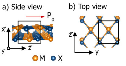
Figure 1: Crystal structure of single-layer MX=GeS, GeSe, SnS, SnSe. The black square indicates the unit cell. The spontaneous electric polarization is in-plane $\mathbf{P}_{0}=P_{0}\mathbf{z}$

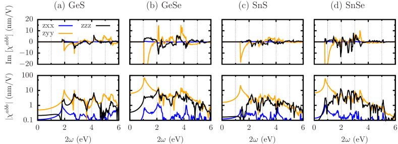
Figure 2: (a)-(d) Second harmonic generation (SHG) tensor $\chi_{2}^{abb}(-2\omega,\omega,\omega)$ for single-layer monochalcogenide MX=GeS, GeSe, SnS, SnSe as a function of outgoing photon frequency $2\omega$. The response can reach $\sim 10$ nm/V in the visible range of frequency which makes them promising for opto-electronic applications.

II Methods

We use density functional theory (DFT) as implemented in the ABINIT Gonze et al. (2009) computer package with the generalized gradient approximation to the exchange correlation energy functional within the Perdew-Burke-Ernzerhof functional Perdew et al. (1996). We use Hartwigsen-Goedecker-Hutter norm conserving pseudopotentials Hartwigsen et al. (1998) available in the ABINIT website abi . We use an energy cut-off of 40 Hartrees to expand the plane waves basis set. To model the slabs we use supercells with 15 Å  along the non-periodic direction, which includes about 10 Å  of vacuum. To calculate the SHG we include 20 valence and 30 conduction bands, together they accounts for all allowed transitions up to 6 eV; we use a mesh of $70\times 70$ $\mathbf{k}$-points along the periodic slab directions.

In periodic-cell calculations, the response is integrated over the three-dimensional (3D) Brillouin zone (BZ). In particular, supercells calculations include a vacuum region used to simulate 2D slabs. This contribution must be subtracted from the total response. To extract the effective response of a single layer we factor the response per unit length perpendicular to the slab and multiply by an effective thickness of layer. The procedure amounts to scale the supercell numerical results by a factor $L/d$, where $L$ is the supercell lattice parameter perpendicular to the slab and $d$ is the effective thickness of the layer. Here we assume reasonable effective slab widths of $d=$2.56, 2.61, 2.84 and 2.73 Å,  for GeS, GeSe, SnS and SnSe, respectively. Once the ground-state wave function and energies are computed, we compute the SHG susceptibility $\chi_{2}$, as implemented TINIBAtin which is based on the analysis of reference Sipe and Shkrebtii, 2000. The sum over $\mathbf{k}$-points is made using the interpolation tetrahedron methodBlöchl et al. (1994). Our calculated band structures agree with previous reports and our method of calculating SHG reproduces that of GaAs reported in the literature Cabellos et al. (2009).

III Results

The electric polarization in materials can be descried as a power series in the electric field Boyd (2008),

$$\mathbf{P}=\mathbf{P_{0}}+\chi_{1}\mathbf{E}+\chi_{2}\mathbf{E}^{2}+\chi_{3}\mathbf{E}^{3}+\cdots,$$ (1)

Where $\mathbf{P}_{0}$ is the electric polarization in the absence of fields, $\chi_{1}$ is the linear susceptibility and $\chi_{2}$, $\chi_{3}$, etc. are the non-linear susceptibilities; $\mathbf{E}$ is the locally-averaged macroscopic electric field (local-field effects are not included in this work). For MX, $\mathbf{P}_{0}=P_{0}\mathbf{z}$ is parallel to the slab as shown in Fig. 1 and can be as large as 1.9 C/m² Rangel et al., 2017. For a monochromatic electric field, $E^{a}=E^{a}(\omega)e^{-i\omega t}$ + c.c., the second order polarization can be expressed as,

$$P^{a}_{2}(t)=\chi^{abc}_{2}(-2\omega;\omega,\omega)E^{b}(\omega)E^{c}(\omega)e^{-i2\omega t}+\textrm{c.c.},$$ (2)

where $a,b$ and $c$ are Cartesian components along $x,y,z$ direction and summation over repeated indices is implied. The space group of bulk MX is $Pnma$, which contains a center of inversion and hence has zero bulk spontaneous polarization. The atoms in the conventional cell are arranged in two weakly coupled layers, each with opposite in-plane polarizations. When one of the layers is removed, the resulting structure lacks inversion symmetry and has large in-plane spontaneous electric polarization Wu and Zeng (2016); Wang and Qian (2017); Rangel et al. (2017).The single-layer of MX has point group $mm2$ and so the only non-zero components of $\chi_{2}$ are $zxx$, $zyy$, $zzz$, $yyz$, $xzx$, as well as the components obtained from exchanging the last two indices.

In Fig. 2 we show our DFT results for the imaginary and absolute part of $\chi_{2}$ for MX=GeS, GeSe, SnS, and SnSe. Only the components giving rise to a current along the polar axis with linear polarization are shown. The other components are much smaller with the exception of $yyz$ which is of the same order as the $zzz$ component. Note that the effective $|\chi_{2}|$ can reach values up to $10$ nm/V over a large frequency range including the visible frequency regime ($1.5$-$3$ eV). In fact, it is larger than that of prototypical semiconductor GaAs Bergfeld and Daum (2003), which can reach up to $0.8$ nm/V, see Fig. 3(a). Another interesting feature is that the strong in-plane anisotropy of $\chi_{2}$ in MX, e.g., $|\chi_{2}^{zyy}|$ is generally larger than $|\chi_{2}^{zzz}|$. In table  1, we compare the reported values of the SHG of other 2D materials studied so far. Even though these materials break inversion symmetry they have a rotational 3-fold symmetry which prevents them from having a polar axis. As a consequence they have zero electric polarization, except for MX studied in this work. Indeed, MX has the largest SHG reported so far.

Monolayer	$|\chi_{2}|$(nm/V)	$\hbar\omega$ (eV)	Ref.	$P_{0}$ (C/m2)
MX	10	0.8-4	present	0.6-1.9 Rangel et al. (2017)
WS2	4.5	3	Janisch et al., 2014(exp.)	0
GaSe	2.4	1	Zhou et al., 2015 (exp.)	0
SiC	0.6	1.5	Attaccalite et al., 2015(th.)	0
MoS2	$0.16$	1.5	Li et al., 2013(exp.)	0
ZnO,GaN	0.08	1.5	Attaccalite et al., 2015(th.)	0
h-BN	0.001	1.5	Li et al., 2013(exp.)	0

Table 1: Reported second harmonic generation (SHG) tensor for various 2D materials. MX stands for GeS, GeSe, SnS or SnSe. Values are meant to be order of magnitude estimates. $\hbar\omega$ is incoming photon energy. A large value of SHG in MoS₂ is reported in Kumar et al., 2013 but has been recently challenged Merano (2016). Note that of the materials studied to date only MX has finite spontaneous electric polarization $P_{0}$ Wu and Zeng (2016); Wang and Qian (2017); Rangel et al. (2017). Experimental (exp.) and theoretical (th.) values are indicated.

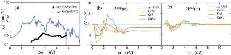
Figure 3: (a) Comparison between experimental SHG tensor in GaAs(001) from Bergfeld and Daum, 2003 and our density functional theory (DFT) calculation for GeSe. The SHG in GeSe is an order of magnitude larger than in GaAs.(b)-(c) Integral of imaginary part of SHG defined in Eq. 10 for the $zyy$ (b) and $zzz$ (c) components. As $\omega$ increases $\mathcal{A}^{zzz}$ vanishes within numerical precision but $\mathcal{A}^{zyy}$ does not. Hence the sum rule Eq. 9 is non-trivially satisfied.

IV Two-band approximation of the SHG susceptibility

Since the analytic expression for $\chi_{2}$ is not simple (even at the single-particle level) it is hard to disentangle the important factors contributing to the magnitude of $\chi_{2}$ or any correlations to other optical responses. However, simple two-band models such as the Rice-Mele model Rice and Mele (1982), have been successful in explaining the relation between shift current and electric polarization Rangel et al. (2017). In this work, we expand this approach and model the SHG along the polar axis, with a two-band approximation. From the general expression for $\chi_{2}$ (see Sipe and Shkrebtii, 2000), setting $a,b,c=z$ and for simplicity omitting the Cartesian components we obtain,

$$\chi_{2}=\chi^{\prime}_{2}+i\chi{{}^{\prime\prime}}_{2},$$ (3)

with,

$$\chi{{}^{\prime}}_{2}=\frac{e^{3}}{\hbar^{2}} \int\frac{dk}{2\pi}\frac{1}{\omega_{21}}|r_{21}|R_{21}\big{[}2H_{+}(\omega_{21},2\omega)$$

$$~{}~{}~{}~{}~{}~{}~{}~{}~{}~{}+\frac{(\omega_{21}-2\omega)}{2\omega}H_{+}(\omega_{21},\omega)\big{]}$$ (4)

$$\chi{{}^{\prime\prime}}_{2}=\frac{1}{2\omega} \big{[}2\sigma_{2}(0;-2\omega,2\omega)-\sigma_{2}(0;-\omega,\omega)\big{]},$$ (5)

where $\sigma_{2}(0;-\omega,\omega)$ is the shift current tensor.

$$\sigma_{2}(0;-\omega,\omega) =\frac{\pi e^{3}}{\hbar^{2}}\int\frac{dk}{2\pi}|r_{21}|^{2}R_{21}\delta(\omega_{21}-\omega).$$ (6)

In these expressions both the positive and negative components of the frequency were taken into account and $\omega$ is positive. The shift vector,

$$R_{21} =\frac{\partial\phi_{21}}{\partial k}+A_{22}-A_{11},$$ (7)

depends on the Berry connections, $A_{nm}=i\langle u_{n}|\partial_{k}|u_{m}\rangle$, where $n,m$ are band indices. $r_{12}=v_{12}/i\omega_{12}$ is the dipole matrix element, and $v_{12}=\langle u_{1}|v|u_{2}\rangle$ are the velocity matrix elements between the periodic part of the Bloch states $u_{m}$. $\phi_{nm}$ is the phase of the interband Berry connection, $A_{nm}=|A_{nm}|e^{-i\phi_{nm}}$. $H_{\pm}(\omega_{nm})$ is

$$H_{\pm}(\omega_{nm},\omega) =\frac{P}{\omega_{nm}-\omega}\pm\frac{P}{\omega_{nm}+\omega},$$ (8)

where $\hbar\omega_{21}=\hbar\omega_{2}-\hbar\omega_{1}=2E_{k}$, $E_{k}$ is the band dispersion and $P$ takes the principal part of the argument. These expressions can also be obtained from Floquet theory Morimoto and Nagaosa (2016). Since $\chi{{}^{\prime\prime}}_{i}$ ($i$=1,2,..) is related to the electromagnetic energy stored in a dielectric Boyd (2008), $\chi{{}^{\prime\prime}}_{2}$ is zero when there is no energy absorption. From Eq. 5 we see that $\chi{{}^{\prime\prime}}_{2}=0$ for $2\hbar\omega<E_{g}$, because two photons of energy at least $\hbar\omega=E_{g}/2$ can be absorbed. The real part however can be non-zero below the gap energy due to virtual transitions.

The imaginary part $\chi{{}^{\prime\prime}}_{2}$ is proportional to the difference of two shift current tensors at the first and second harmonic of the incoming photon frequency. From previous studies we know the shift current tensor Cook et al. (2017); Tan et al. (2016) has sharp onset at the band edges. Hence $\chi{{}^{\prime\prime}}_{2}$ has two sharp peaks at $\hbar\omega=E_{g}$ and $2\hbar\omega=E_{g}$. Barring a fortuitous cancellation between the peaks, a large shift current would imply large $\chi{{}^{\prime\prime}}_{2}$. More important, the shift current tensor in Eq. 6 depends on a gauge-invariant matrix elements $|r_{12}|^{2}R_{12}$ and the density of states (DOS). Usually, these contributions cannot be disentangled and the shift current has a complex dependence of each of them Young and Rappe (2012); Tan et al. (2016). In 2D, the situation is different. The DOS is approximately constant and hence the shift current (and $\chi_{2}$) are determined by the shift vector and velocity matrix elements Fregoso et al. (2017). This means that, for materials with similar DOS, the one with larger spontaneous electric polarization have larger shift current and hence stronger SHG. As shown above our DFT calculations of the SHG in MX are consistent with this picture.

IV.1 Sum rule

Integrating the imaginary part of $\chi_{2}$, as given in Eq. 5 we obtain,

$$\int_{0}^{\infty}d\omega~{}2\omega~{}\chi{{}^{\prime\prime}}_{2}(-2\omega,\omega,\omega)=0,$$ (9)

where we used $r_{21}=v_{21}/i\omega_{21}$. This result is not a simple consequence of the oddness of $\chi^{{}^{\prime\prime}}_{2}$ under $\omega\to-\omega$ and hence it is interesting to assess its validity for a full-band structure calculation. To this end we define,

$$\mathcal{A}^{zzz}(\omega)=\int_{0}^{\omega}d\Omega~{}2\Omega~{}\chi^{{}^{\prime\prime}zzz}_{2},$$ (10)

and computed $\mathcal{A}^{zzz}(\omega)$ within DFT. We find the sum rule is mostly satisfied for $\omega>7$ eV for the materials considered, as shown in Fig. 3(c). The sum rule is not satisfied for other components; for instance in Fig. 3(b) we show $\mathcal{A}^{zyy}$. Hence the two-band approximation captures the integrated SHG response along the polar axis in MX.

V conclusions

We have calculated the second harmonic generation (SHG) susceptibility of single-layer GeS, GeSe, SnS and SnSe using density functional theory. We found that the effective 3D SHG response of these materials is larger than that of GaAs by an order of magnitude and is the largest reported so far. In addition, we constructed a two-band approximation to SHG multiband susceptibility to describe the SHG. Within this approximation we found that the imaginary part of $\chi_{2}^{zzz}$ is proportional to the difference of two shift current tensors at the first and second harmonic frequencies. Since the shift current is large in MXRangel et al. (2017); Cook et al. (2017), we expect the SHG will be large too, in agreement with our DFT calculation.

We left for future research the inclusion of quasiparticle effects, local fields and excitonic contributions. Quasiparticle and local fields effects are expected to be small and could be well approximated within the independent-particle formalism Luppi et al. (2016). Excitonic bound states, on the other hand, are expected to increase $|\chi_{2}|$ due to resonances at bound states. In conclusion, the strong SHG together with the large shift current in GeS, GeSe, SnS and SnSe make these materials of great interest for optoelectronic applications.

VI acknowledgments

We thank T. Rangel and C. Salazar for their help with TINIBA and ABINIT and M. Merano for kindly bringing to our attention reference Merano, 2016. We acknowledge support from NERSC contract No. DE-AC02-05CH11231.

References

- Boyd (2008) R. W. Boyd, Nonlinear Optics (Academic Press, 2008).
- Aspnes (1972) D. E. Aspnes, Phys. Rev. B 6, 4648 (1972).
- Levine (1990) Z. H. Levine, Phys. Rev. B 42, 3567 (1990).
- Sipe and Ghahramani (1993) J. E. Sipe and E. Ghahramani, Phys. Rev. B 48, 11705 (1993).
- Aversa and Sipe (1995) C. Aversa and J. E. Sipe, Phys. Rev. B 52, 14636 (1995).
- Sipe and Shkrebtii (2000) J. E. Sipe and A. I. Shkrebtii, Phys. Rev. B 61, 5337 (2000).
- Luppi et al. (2016) E. Luppi, , and V. Veniard, Semicond. Sci. Technol. 31, 123002 (2016).
- Kumar et al. (2013) N. Kumar, S. Najmaei, Q. Cui, F. Ceballos, P. M. Ajayan, J. Lou, and H. Zhao, Phys. Rev. B 87, 161403 (2013).
- Li et al. (2013) Y. Li, Y. Rao, K. F. Mak, Y. You, S. Wang, C. R. Dean, and T. F. Heinz, Nano Letters 13, 3329 (2013).
- Kim et al. (2013) C.-J. Kim, L. Brown, M. W. Graham, R. Hovden, R. W. Havener, P. L. McEuen, D. A. Muller, and J. Park, Nano Letters 13, 5660 (2013).
- Janisch et al. (2014) C. Janisch, Y. Wang, D. Ma, N. Mehta, A. L. Elias, N. Perea-Lopez, M. Terrones, V. Crespi, and Z. Liua, Scientific Reports 4, 5530 (2014).
- Malard et al. (2013) L. M. Malard, T. V. Alencar, A. P. M. Barboza, K. F. Mak, and A. M. de Paula, Phys. Rev. B 87, 201401 (2013).
- Zhou et al. (2015) X. Zhou, J. Cheng, Y. Zhou, T. Cao, H. Hong, Z. Liao, S. Wu, H. Peng, K. Liu, and D. Yu, Journal of the American Chemical Society 137, 7994 (2015).
- Attaccalite et al. (2015) C. Attaccalite, A. Nguer, E. Cannuccia, and M. Gruning, Phys. Chem. Chem. Phys. 17, 9533 (2015).
- Chang et al. (2016) K. Chang, J. Liu, H. Lin, N. Wang, K. Zhao, A. Zhang, F. Jin, Y. Zhong, X. Hu, W. Duan, Q. Zhang, L. Fu, Q.-K. Xue, X. Chen, and S.-H. Ji, Science 353, 274 (2016).
- Mehboudi et al. (2016) M. Mehboudi, A. M. Dorio, W. Zhu, A. van der Zande, H. O. H. Churchill, A. A. Pacheco-Sanjuan, E. O. Harriss, P. Kumar, , and S. Barraza-Lopez, Nano Lett. 16, 1704 (2016).
- Wu and Zeng (2016) M. Wu and X. C. Zeng, Nano Letters 16, 3236 (2016).
- Wang and Qian (2017) H. Wang and X. Qian, 2D Materials 4, 015042 (2017).
- Rangel et al. (2017) T. Rangel, B. M. Fregoso, B. S. Mendoza, T. Morimoto, J. E. Moore, and J. B. Neaton, Phys. Rev. Lett. 119, 067402 (2017).
- Cook et al. (2017) A. M. Cook, B. M. Fregoso, F. de Juan, S. Coh, and J. E. Moore, Nature Communications 8, 14176 (2017).
- Fregoso et al. (2017) B. M. Fregoso, T. Morimoto, and J. E. Moore, Phys. Rev. B 96, 075421 (2017).
- von Rohr et al. (2017) F. O. von Rohr, H. Ji, F. A. Cevallos, T. Gao, N. P. Ong, and R. J. Cava, Journal of the American Chemical Society 139, 2771 (2017).
- von Baltz and Kraut (1981) R. von Baltz and W. Kraut, Phys. Rev. B 23, 5590 (1981).
- Sturman and Sturman (1992) B. I. Sturman and P. J. Sturman, Photovoltaic and Photo-refractive Effects in Noncentrosymmetric Materials (CRC Press, 1992).
- Young and Rappe (2012) S. M. Young and A. M. Rappe, Phys. Rev. Lett. 109, 116601 (2012).
- Tan et al. (2016) L. Z. Tan, F. Zheng, S. M. Young, F. Wang, S. Liu, and A. M. Rappe, Npj Computational Materials 2, 16026 (2016).
- Gonze et al. (2009) X. Gonze et al., Computer Physics Communications 180, 2582 (2009).
- Perdew et al. (1996) J. P. Perdew, K. Burke, and Y. Wang, Phys. Rev. B 54, 16533 (1996).
- Hartwigsen et al. (1998) C. Hartwigsen, S. Goedecker, and J. Hutter, Phys. Rev. B 58, 3641 (1998).
- (30) www.abinit.org.
- (31) TINIBA is a tool written in bash, perl, and fortran to compute optical responses based on the ABINIT. https://github.com/bemese/tiniba.
- Blöchl et al. (1994) P. E. Blöchl, O. Jepsen, and O. K. Andersen, Phys. Rev. B 49, 16223 (1994).
- Cabellos et al. (2009) J. L. Cabellos, B. S. Mendoza, M. A. Escobar, F. Nastos, and J. E. Sipe, Phys. Rev. B 80, 155205 (2009).
- Bergfeld and Daum (2003) S. Bergfeld and W. Daum, Phys. Rev. Lett. 90, 036801 (2003).
- Merano (2016) M. Merano, Opt. Lett. 41, 187 (2016).
- Rice and Mele (1982) M. J. Rice and E. J. Mele, Phys. Rev. Lett. 49, 1455 (1982).
- Morimoto and Nagaosa (2016) T. Morimoto and N. Nagaosa, Science Advances 2 (2016).