Geometry-Oblivious FMM for Compressing Dense SPD Matrices

Abstract.

We present GOFMM (geometry-oblivious FMM), a novel method that creates a hierarchical low-rank approximation, or “compression,” of an arbitrary dense symmetric positive definite (SPD) matrix. For many applications, GOFMM enables an approximate matrix-vector multiplication in $N\log N$ or even $N$ time, where $N$ is the matrix size. Compression requires $N\log N$ storage and work. In general, our scheme belongs to the family of hierarchical matrix approximation methods. In particular, it generalizes the fast multipole method (FMM) to a purely algebraic setting by only requiring the ability to sample matrix entries. Neither geometric information (i.e., point coordinates) nor knowledge of how the matrix entries have been generated is required, thus the term “geometry-oblivious.” Also, we introduce a shared-memory parallel scheme for hierarchical matrix computations that reduces synchronization barriers. We present results on the Intel Knights Landing and Haswell architectures, and on the NVIDIA Pascal architecture for a variety of matrices.

1. Introduction

We present GOFMM, a novel algorithm for the approximation of dense symmetric positive definite (SPD) matrices. GOFMM can be used for compressing a dense matrix and accelerating matrix-vector multiplication operations. As an example, in Figure 1 we report timings for an SGEMM operation using an optimized dense matrix library and compare with the GOFMM-compressed version.

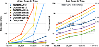
Figure 1. Comparison of runtime in seconds (y-axis) versus problem size $N$ (x-axis) to multiply test matrix K02 (see §3) of size $N\times N$ with a matrix of size $N\times r$, for $r=512,1024,2048$. Results are plotted against a linear scale (left) and a logarithmic scale (right). The top three curves demonstrate ${\mathcal{O}}(N^{2})$ scaling of Intel MKL SGEMM for each value of $r$. The middle curve shows the time for GOFMM to compress K02, which scales as ${\mathcal{O}}(N\log{N})$ in these cases. The bottom three curves show the ${\mathcal{O}}(N)$ scaling of the time for GOFMM to evaluate the matrix product for each value of $r$ after compression is already completed. The GOFMM results reach accuracies of $110-2$ to $410-4$ in single precision. In these experiments, the crossover (including compression time) is $N=$16\,384$$, and for $N=$147\,456$$, we observe an 18$\times$ speedup over SGEMM.

Let $K\in\mathbb{R}^{N\times N}$ be a dense SPD matrix, with $K=K^{T}$ and $x^{T}Kx>0,\ \forall x\in\mathbb{R}^{N},\ x\neq 0$. Since $K$ is dense it requires $\operatorname{\mathcal{O}}(N^{2})$ storage and $\operatorname{\mathcal{O}}(N^{2})$ work for a matrix-vector multiplication (hereby “matvec”). Using $\operatorname{\mathcal{O}}(N\log N)$ memory and work, we construct an approximation $\tilde{K}$ such that $\|\tilde{K}-K\|\leq\epsilon\|K\|$, where $\epsilon$ is a user-defined error tolerance. Assuming the evaluation of a single matrix entry $K_{ij}$ requires $\operatorname{\mathcal{O}}(1)$ work, a matvec with $\tilde{K}$ requires $\operatorname{\mathcal{O}}(N\log N)$ or $\operatorname{\mathcal{O}}(N)$ work depending on the properties of $K$ and the GOFMM variant. Our scheme belongs to the class of hierarchical matrix approximation methods.

Problem statement: given any SPD matrix $K$, our task is to construct a hierarchically low-rank matrix $\tilde{K}$ so that $\|K-\tilde{K}\|/\|K\|$ is small. The only required input to our algorithm is a routine that returns $K_{IJ}$, for arbitrary row and column index sets $I$ and $J$. The constant in the complexity estimate depends on the structure of the underlying matrix. Let us remark and emphasize that our scheme cannot guarantee both accuracy and work complexity simultaneously since an arbitrary SPD matrix may not admit a good hierarchical matrix approximation (see  §2).

We say that a matrix $\tilde{K}$ has a hierarchically low-rank structure, i.e., $\tilde{K}$ is an $\mathcal{H}\!$-matrix (Hackbusch, 2015; Bebendorf, 2008), if

(1) $$\tilde{K}=D+S+UV,$$

where $D$ is block-diagonal with every block being an $\mathcal{H}\!$-matrix, $U$ and $V$ are low rank, and $S$ is sparse. At the base case of this recursive definition, the blocks of $D$ are small dense matrices. An $\mathcal{H}\!$-matrix matvec requires $\operatorname{\mathcal{O}}(N\log N)$ work the constant depending on the rank of $U$ and $V$. Depending on the construction algorithm, this complexity can go down to $\operatorname{\mathcal{O}}(N)$. Although such matrices are rare in real-world applications, it is quite common to find matrices that can be approximated arbitrarily well by an $\mathcal{H}\!$-matrix.

One important observation is that this hierarchical low-rank structure is not invariant to row and column permutations. Therefore any algorithm for constructing $\tilde{K}$ must first appropriately permute $K$ before constructing the matrices $U,V,D$, and $S$. Existing algorithms rely on the matrix entries $K_{ij}$ being “interactions” (pairwise functions) between points $\{x_{i}\}_{i=1}^{N}$ in $\mathbb{R}^{d}$ and permute $K$ either by clustering the points (typically using some tree data-structure) or by using graph partitioning techniques (if $K$ is sparse). GOFMM does not require such geometric information.

Background and significance

Dense SPD matrices appear in scientific computing, statistical inference, and data analytics. They appear in Cholesky and LU factorization (Grasedyck et al., 2008), in Schur complement matrices for saddle point problems (Benzi et al., 2005), in Hessian operators in optimization (Muske and Howse, 2001), in kernel methods for statistical learning (Hofmann et al., 2008; Gray and Moore, 2001), and in N-body methods and integral equations (Greengard, L., 1994; Hackbusch, 2015). In many applications, the entries of the input matrix $K$ are given by $K_{ij}=\mathcal{K}(x_{i},x_{j}):\mathbb{R}^{d}\times\mathbb{R}^{d}\rightarrow\mathbb{R}$, where $\mathcal{K}$ is a kernel function. Examples of kernel functions are radial basis functions, Green’s functions, and angle similarity functions. For such kernel matrices, the input is not a matrix, but only the points $\{x_{i}\}_{i=1}^{N}$. The points are used to appropriately permute the matrix using spatial data structures. Furthermore, the construction of the sparse correction $S$ uses nearest-neighbor structure of the input points. The low-rank matrices $U,V$ can be either analytically computed using expansions of the kernel function, or semi-algebraically computed using fictitious points (or equivalent points), or using algebraic sampling-based methods that use geometric information. In a nutshell, geometric information is used in all aspects of an $\mathcal{H}\!$-matrix method.

In many cases however, such points and kernel functions are not available. For example, in dense graphs in data analysis (e.g., social networks, protein interactions). Related matrices include graph Laplacian operators and their inverses. Additional examples include frontal matrices and Schur complements in factorization of sparse matrices; Hessian operators in optimization; and kernel methods in machine learning without points (e.g., word sequences and diffusion on graphs (Cancedda et al., 2003; Kondor and Lafferty, 2002)).

Contributions

GOFMM is inspired by the rich literature of algorithms for matrix sketching, hierarchical matrices, and fast multipole methods. Its unique feature is that by using only matrix evaluations it generalizes FMM ideas to compressing arbitrary SPD matrices. In more detail, our contributions are summarized below.

• A result from reproducing kernel Hilbert space theory is that any SPD matrix corresponds to a Gram matrix of vectors in some, unknown Gram (or feature) space (Hofmann et al., 2008). Based on this result, the matrix entries are inner products, which we use to define distances. These distances allow us to design an efficient, purely algebraic FMM method.

• The key algorithmic components of GOFMM (and other hierarchical matrix and FMM codes) are tree traversals. We test parallel level-by-level traversals, out-of-order traversals using OpenMP’s advanced task scheduling and an in-house tree-task scheduler. We found that scheduling significantly improves the performance when compared to level-by-level tree traversals. We also use this scheduling to support heterogeneous architectures.

• We conduct extensive experiments to demonstrate the feasibility of the proposed approach. We test our code on 22 different matrices related to machine learning, stencil PDEs, spectral PDEs, inverse problems, and graph Laplacian operators. We perform numerical experiments on Intel Haswell and KNL, Qualcomm ARM, and NVIDIA Pascal architectures. Finally, we compare with three state-of-the-art codes: HODLR, STRUMPACK, and ASKIT.

GOFMM also has several additional capabilities. If points and kernel functions (or Green’s) function are available, they can be utilized in a similar way to the algebraic FMM code ASKIT described in (March et al., 2015c, a). GOFMM currently supports three different measures of distance: geometric point-based (if available), Gram-space $\ell^{2}$ distance, and Gram-space angle distance. GOFMM has support for matvecs with multiple vectors, which is useful for Monte-Carlo sampling, optimization, and block Krylov methods.

Limitations

GOFMM is restricted to SPD matrices. (However, if we are given points, the method becomes similar to existing methods). GOFMM guarantees symmetry of $\tilde{K}$, but if $\|K-\tilde{K}\|/\|K\|$ is large, positive definiteness may be compromised. To reiterate, GOFMM cannot simultaneously guarantee both accuracy and work complexity. This initial implementation of GOFMM supports shared-memory parallelism and accelerators, but not distributed memory architectures. The current version of GOFMM also has several parameters that require manual tuning. Often, the main goal of building $\mathcal{H}\!$-matrix approximations is to construct a factorization of $K$, a topic we do not discuss in this paper. Our method requires the ability to evaluate kernel entries and the complexity estimates require that these entries can be computed in $\operatorname{\mathcal{O}}(1)$ time. If $K$ is only available through matrix-free interfaces, these assumptions may not be satisfied. Other algorithms, like STRUMPACK, have inherent support for such matrix-free compression.

Related work.

The literature on hierarchical matrix methods and fast multipole methods is vast. Our discussion is brief and limited to the most related work.

Low-rank approximations. The most popular approach for compressing arbitrary matrices is a global low-rank approximation using randomized linear algebra. In (1), this is equivalent to setting $D$ and $S$ to zero and constructing only $U$ and $V$. Examples include the CUR (Mahoney and Drineas, 2009) factorization, the Nystrom approximation (Williams and Seeger, 2001), the adaptive cross approximation (Bebendorf and Rjasanow, 2003), and randomized rank-revealing factorizations (Martinsson et al., 2010; Halko et al., 2011). These techniques can also be used for $\mathcal{H}\!$-matrix approximations when $D$ is not zero. Instead of applying them to $K$, we can apply them to the off-diagonal blocks of $K$. FMM-specific techniques that are a mix between analytic and algebraic methods include kernel-independent methods (Martinsson and Rokhlin, 2007; Ying et al., 2004) and the black-box FMM (Fong and Darve, 2009). Constructing both $U$ and $V$ accurately and with optimal complexity is hard. The most robust algorithms require $\operatorname{\mathcal{O}}(N^{2})$ complexity or higher (randomized methods and leverage-score sampling) since they require one to “touch” all the entries of the matrix (or block) to be approximated.

Permuting the matrix. When $K$ is sparse, the method of choice uses graph-partitioning. This doesn’t scale to dense matrices because practical graph partitioning algorithms scale at least linearly with the number of edges and thus the construction cost would be at least $\operatorname{\mathcal{O}}(N^{2})$ (Agullo et al., 2016; Karypis and Kumar, 1998).

$\mathcal{H}\!$-matrix methods and software. Treecodes and fast multipole methods originally were developed for N-body problems and integral equations. Algebraic variants led the way to the abstraction of $\mathcal{H}\!$-matrix methods and the application to the factorization of sparse systems arising from the discretization of elliptic PDEs (Hackbusch, 2015; Bebendorf, 2008; Ambikasaran, 2013; Greengard et al., 2009; Ho and Greengard, 2012; Xia et al., 2010).

Let us briefly summarize the $\mathcal{H}\!$-matrix classification. Recall the decomposition $K=D+UV+S$, (1). If $S$ is zero the approximation is called a hierarchically off-diagonal low rank (HODLR) scheme. In addition to $S$ being zero, if the $\mathcal{H}\!$-matrix decomposition of $D$ is used to construct $U$, $V$ we have a hierarchically semi-separable (HSS) scheme. If $S$ is not zero we have a generic $\mathcal{H}\!$-matrix; but if the $U,V$ terms are constructed in a nested way then we have an $\mathcal{H}^{2}$-matrix or an FMM depending on more technical details. HSS and HODLR matrices lead to very efficient approximation algorithms for $K^{-1}$. However, ${\mathcal{H}}^{2}$ and FMM compression schemes better control the maximum rank of the $U$ and $V$ matrices than HODLR and HSS schemes. For the latter, the rank of $U$ and $V$ can grow with $N$ (Chandrasekaran et al., 2010) and the complexity bounds are no longer valid. Recently, here have been algorithms to effectively compress FMM and ${\mathcal{H}}^{2}$-matrices (Coulier et al., 2016; Yokota et al., 2016).

METHOD	MATRIX	LOW-RANK	PERM	$S$
FMM (Cheng et al., 1999)	$\mathcal{K}(x_{i},x_{j})$	EXP	OCTREE	Y
KIFMM (Ying et al., 2004)	$\mathcal{K}(x_{i},x_{j})$	EQU	OCTREE	Y
BBFMM (Fong and Darve, 2009)	$\mathcal{K}(x_{i},x_{j})$	EQU	OCTREE	Y
HODLR (Ambikasaran and Darve, 2013)	$K_{ij}$	ALG	NONE	N
STRUMPACK (Rouet et al., 2016)	$K_{ij}$	ALG	NONE	N
ASKIT (March et al., 2016)	$\mathcal{K}(x_{i},x_{j})$	ALG	TREE	Y
MLPACK (Curtin et al., 2013)	$\mathcal{K}(x_{i},x_{j})$	EQU	TREE	Y
GOFMM	$K_{ij}$	ALG	TREE	Y

Table 1. We summarize the main features of different $\mathcal{H}\!$-matrix methods/codes for dense matrices. “MATRIX” indicates whether the method requires a kernel function and points—indicated by $\mathcal{K}(x_{i},x_{j})$—or it just requires kernel entries—indicated by $K_{ij}$. “LOW-RANK” indicates the method used for the off-diagonal low-rank approximations: “EXP” indicates kernel function-dependent analytic expansions; “EQU” indicates the use of equivalent points (restricted to low $d$ problems); “ALG” indicates an algebraic method. “PERM” indicates the permutation scheme used for dense matrices: “OCTREE” indicates that the scheme doesn’t generalize to high dimensions; “NONE” indicates that the input lexicographic order is used; and “TREE” indicates geometric partitioning that scales to high dimensions. $S$ indicates whether a sparse correction (FMM or ${\mathcal{H}^{2}}$) is supported. In §4, we present comparisons with ASKIT, STRUMPACK, and HODLR.

One of the most scalable methods is STRUMPACK (Ghysels et al., 2016; Rouet et al., 2016; Martinsson, 2016), which constructs an HSS approximation of a square matrix (not necessarily SPD) and then uses it to construct an approximate factorization. For dense matrices STRUMPACK uses the lexicographic ordering. If no fast matrix-vector multiplication is available, STRUMPACK requires $\operatorname{\mathcal{O}}(N^{2})$ work for compressing a dense SPD matrix, and $\operatorname{\mathcal{O}}(N)$ work for the matvec.

2. Methods

Given $K\in\mathbb{R}^{N\times N}$, GOFMM aims to construct an $\mathcal{H}\!$-matrix ${\widetilde{K}}$ in the form of (1) such that we can approximate

(2) $$u=Kw\approx{\widetilde{K}}w,\ \mbox{~{}for~{}}\ w\in\mathbb{R}^{N}.$$

When points $\{x_{i}\}^{N}_{i=1}$ are available such that $K_{ij}=\mathcal{K}(x_{i},x_{j})$, the recursive partitioning on $D$ and the low-rank structure $UV$ use distances between $x_{i}$ and $x_{j}$. Existing FMM methods approximate $K_{ij}$ when $x_{i}$ and $x_{j}$ are sufficiently far from each other. Otherwise, $K_{ij}$ is not approximated and it is placed either in $D$ or in $S$. We call this distance-based criterion near-far pruning.

To define such a pruning scheme without $\{x_{i}\}^{N}_{i=1}$, we need a notion of distance between two matrix indices $i$ and $j$. We define such a distance in the next section. With it, we can permute $K$ and define neighbors for each index $i$. In §2.2, we describe a task-based algebraic FMM that only relies on the distance we define. Finally in §2.3, we discuss task parallelism and scheduling.

2.1. Geometry-oblivious techniques

In this section, we introduce the machinery for using GOFMM in a geometry-oblivious manner. Throughout the following discussion, we refer to a set of indices $\mathcal{I}=\{1,\dots,N\}$, where index $i$ corresponds to the $i$th row (or column) of the matrix $K$ in the original ordering. Our objective is to find a permutation of $\mathcal{I}$ so that $K$ can be approximated by an $\mathcal{H}\!$-matrix. The key is to define a distance between a pair of indices $i,j\in\mathcal{I}$, denoted as $d_{ij}$. Using the distances, we then perform a hierarchical clustering of $\mathcal{I}$, which is used to define the permutation, and determine which interaction go into the sparse correction $S$ (using nearest neighbors).

Three measures of distance.

We will define the point-based Euclidean distance, a Gram-space Euclidean distance, and a Gram-space angle distance.

Geometric-$\ell^{2}$. If we are given points $\{x_{i}\}_{i=1}^{N}$, then $d_{ij}=\lVert x_{i}-x_{j}\rVert_{2}$ is the geometric $\ell^{2}$ distance. This will be the geometry-aware reference implementation for cases where points are given.

Gram-$\ell^{2}$ (or “kernel” distance). Since $K$ is SPD, it is the Gram matrix of some set of unknown Gram vectors, $\{\phi_{i}\}_{i=1}^{N}\subset\mathbb{R}^{N}$ ( (Schölkopf and Smola, 2002), proposition 2.16, page 44). That is, $K_{ij}=(\phi_{i},\phi_{j})$, where $(\cdot,\cdot)$ denotes the $\ell^{2}$ inner product in $\mathbb{R}^{N}$. Then we define the Gram $\ell^{2}$ distance as $d_{ij}=\lVert\phi_{i}-\phi_{j}\rVert$. Computing the kernel distance only requires three entries of $K$:

(3) $$d_{ij}^{2}=\lVert\phi_{i}\rVert^{2}+\lVert\phi_{j}\rVert^{2}-2(\phi_{i},\phi_{j})=K_{ii}+K_{jj}-2K_{ij}.$$

Gram angles (or “angle” distance). Our third measure of distance considers angles between Gram vectors, which is based on the standard sine distance (cosine similarity) in inner product spaces. We define the Gram angle distance as $d_{ij}=\sin^{2}\left(\angle(\phi_{i},\phi_{j})\right)\in[0,1]$. This expression is chosen so that $d_{ij}$ is small for nearly collinear Gram vectors, large for nearly orthogonal Gram vectors, and $d_{ij}$ is inexpensive to compute. Although the value $d_{ij}$ may seem arbitrary, we only compare values for the purpose of ordering, so any equivalent metric will do. Computing an angle distance only requires three entries of $K$:

(4) $$d_{ij}=1-\cos^{2}\left(\angle(\phi_{i},\phi_{j})\right)=1-K_{ij}^{2}/(K_{ii}K_{jj}).$$

To reiterate for emphasis, $d_{ij}$ define proper distances (metrics) because $K$ is SPD. And with distances, we can apply FMM.

Tree partitioning and nearest neighbor searches

$K$ is permuted using a balanced binary tree. The root node is assigned the full set of points, and the tree is constructed recursively by splitting a node’s points evenly between two child nodes. The splitting terminates at nodes with some pre-determined leaf size $m$. The leaf nodes then define a partial ordering of the indices: if leaf $\alpha$ is anywhere to the left of leaf $\beta$, then the indices of $\alpha$ precede those of $\beta$. We use this ordering to permute rows and columns of $K$. In the remainder of this paper, we use the notation $\alpha,\beta$ to refer interchangeably to a node or the set of indices belonging to the node.

Algorithm 2.1 $[{\tt l},{\tt r}]=\texttt{metricSplit}(\alpha)$

  $p=\mbox{argmax}\,(\{d_{ic}\lvert i\in\alpha\})$; $q=\mbox{argmax}(\{d_{ip}\lvert i\in\alpha\})$;

  $[{\tt l},{\tt r}]=\mbox{medianSplit}(\{d_{ip}-d_{iq}\lvert i\in\alpha\})$;

In our implementation, we use a ball tree (March et al., 2016). For geometric distances it costs $\operatorname{\mathcal{O}}(N\log N)$. But Gram distances require sampling to avoid $\operatorname{\mathcal{O}}(N^{2})$ costs. Suppose we use one of the Gram distances to split an interior node $\alpha$ between its left child ${\tt l}$ and right child ${\tt r}$. We define $c=\frac{1}{n_{\rm{c}}}\sum\phi_{i}$ to be an approximate centroid taken over a small sample of $n_{\rm{c}}$ Gram vectors belonging to $\alpha$. $n_{\rm{c}}$ is $\operatorname{\mathcal{O}}(1)$. Next, we find the point $p$ that is farthest away in distance from $c$, and the point $q$ that is farthest away from $p$. Then we split the indices $i\in\alpha$ on the values $d_{ip}-d_{iq}$, which measures the degree to which $i$ is closer to $p$ than to $q$. This approach is outlined in Algorithm 2.1.

We perform all nearest neighbors (ANN) search using randomized trees that are constructed in exactly the same way as the partitioning tree, except that $p$ and $q$ are chosen randomly. The search algorithm is described in (Xiao and Biros, 2016) and (briefly) in the next section.

2.2. Algebraic Fast Multipole Method

$\mathcal{H}\!$-matrix methods (including algebraic FMM) have two phases: compression and evaluation. As we discussed in the introduction, $K$ is compressed recursively using a binary tree such that

(5) $${\widetilde{K}}_{\alpha\alpha}=\begin{bmatrix}{\widetilde{K}}_{{\tt l}{\tt l}}&0\\ 0&{\widetilde{K}}_{{\tt r}{\tt r}}\\ \end{bmatrix}+\begin{bmatrix}0&S_{{\tt l}{\tt r}}\\ S_{{\tt r}{\tt l}}&0\\ \end{bmatrix}+\begin{bmatrix}0&UV_{{\tt l}{\tt r}}\\ UV_{{\tt r}{\tt l}}&0\\ \end{bmatrix},$$

where ${\tt l}$ and ${\tt r}$ are left and right child of the treenode $\alpha$. Each node $\alpha$ contains a set of matrix indices and the two children evenly split the indices such that $\alpha={\tt l}\cup{\tt r}$. (We overload the notation $\alpha$, $\beta$, ${\tt l}$ and ${\tt r}$ to denote the matrix indices that those treenode own.) In Figure 2, the blue blocks depict $S$ (at all levels) and $D$ (in the leaf level), and the pink blocks depict the $UV$ matrices.

We use four tree traversals to describe the algorithms in GOFMM: postorder (POST), preorder (PRE), any order (ANY), and any order-leaves only (LEAF). By “task” we refer to a computation that occurs when we visit a tree node during a traversal. We list all tasks required by Algorithm 2.2 and Algorithm 2.7 in Table 2.

We start by creating the binary metric ball tree in Algorithm 2.2 that represents the binary partitioning (and encodes a symmetric permutation of matrix $K$). This requires the distance metric $d_{ij}$ and a preorder traversal (PRE) of the first task SPLI($\alpha$) in Table 2.

Task	Operations	FLOPS
SPLI($\alpha$)	split $\alpha$ into ${\tt l}$ and ${\tt r}$ Algorithm 2.1	$\lvert\alpha\rvert$
ANN($\alpha$)	update ${\mathcal{N}}_{\alpha}$ with KNN($K_{\alpha\alpha}$)	$m^{2}$
SKEL($\alpha$)	${\widetilde{\alpha}}$ in Algorithm 2.6	$2s^{3}+2m^{3}$
COEF($\alpha$)	$P_{{\widetilde{\alpha}}\alpha}$ or $P_{{\widetilde{\alpha}}[{\widetilde{{\tt l}}}{\widetilde{{\tt r}}}]}$ in Algorithm 2.6	$s^{3}$
N2S($\alpha$)	if $\alpha$ is leaf then ${\widetilde{w}}_{\alpha}=P_{{\widetilde{\alpha}}\alpha}w_{\alpha}$	$2msr$
	else ${\widetilde{w}}_{\alpha}=P_{{\widetilde{\alpha}}[{\widetilde{{\tt l}}}{\widetilde{{\tt r}}}]}[{\widetilde{w}}_{{\tt l}};{\widetilde{w}}_{{\tt r}}]$	$2s^{2}r$
SKba($\beta$)	$\forall\alpha\in\mathtt{Far}(\beta)$, $K_{{\widetilde{\beta}}{\widetilde{\alpha}}}=K({\widetilde{\beta}},{\widetilde{\alpha}})$	$ds^{2}\lvert\mathtt{Far}(\beta)\rvert$
S2S($\beta$)	${\widetilde{u}}_{\beta}=\sum_{\alpha\in\mathtt{Far}(\beta)}K_{{\widetilde{\beta}}{\widetilde{\alpha}}}{\widetilde{w}}_{\alpha}$	$2s^{2}r\lvert\mathtt{Far}(\beta)\rvert$
S2N($\beta$)	if $\alpha$ is leaf then $u_{\beta}=P_{{\widetilde{\beta}}\beta}^{T}{\widetilde{u}}_{\beta}$	$2msr$
	else $[{\widetilde{u}}_{{\tt l}};{\widetilde{u}}_{{\tt r}}]+=P_{{\widetilde{\beta}}[{\widetilde{{\tt l}}}{\widetilde{{\tt r}}}]}^{T}{\widetilde{u}}_{\beta}$	$2s^{2}r$
Kba($\beta$)	$\forall\alpha\in\mathtt{Near}(\beta)$, $K_{\beta\alpha}=K(\beta,\alpha)$	$m^{2}\lvert\mathtt{Near}(\beta)\rvert$
L2L($\beta$)	$u_{\beta}+=\sum_{\alpha\in\mathtt{Near}(\beta)}K_{\beta\alpha}w_{\alpha}$	$2m^{2}r\lvert\mathtt{Near}(\beta)\rvert$

Table 2. Tasks and their costs in FLOPS. SPLI (tree splitting), ANN (all nearest-neighbors), SKEL (skeletonization), COEF (interpolation) SKba and Kba (caching submatrices) occur in the compression phase. Interactions N2S (nodes to skeletons), S2S (skeletons to skeletons), S2N (skeletons to nodes), and L2L (leaves to leaves) occur in the evaluation phase.

Algorithm 2.2 Compress($K$)

1:  for each randomized tree do # iterative neighbor search

2:       (PRE) SPLI($\alpha$) # create a random projection tree

3:       (LEAF) ANN($\alpha$) # search $\kappa$ neighbors in leaf nodes

4:  (PRE) SPLI($\alpha$) # create a metric ball tree

5:  (LEAF) LeafNear($\beta$) # build Near$(\beta)$ using ${\mathcal{N}}(\beta)$

6:  (LEAF) FindFar($\beta$,root) # find Far$(\beta)$ using MortonID

7:  (POST) MergeFar($\alpha$) # merge Far$({\tt l})$, Far$({\tt r})$ to Far$(\alpha)$

8:  (POST) SKEL($\alpha$) # compute skeletons ${\widetilde{\alpha}}$

9:  (ANY) COEF($\alpha$) # compute the coefficient matrix $P$

10:  (ANY) Kba($\beta$) # optionally evaluate and cache $K_{\beta\alpha}$

11:  (ANY) SKba($\beta$) # optionally evaluate and cache $K_{{\widetilde{\beta}}{\widetilde{\alpha}}}$

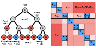
Figure 2. A partitioning tree (left) and corresponding hierarchically low-rank plus sparse matrix (right). The off-diagonal blocks are combinations of low-rank matrices (pink) and sparse matrices (blue). The $\bigstar$ symbol denotes an entry that cannot be approximated (because the corresponding interaction is between neighbors). The solid edges in the tree mark the path traversed by FindFar($\beta$,0). Since $K_{\beta\alpha}$ does not contain any neighbor interactions ($\bigstar$), this traversal adds $\alpha$ to Far$(\beta)$. In this example, FindFar(l,0) computes Far$({\tt l})=\{{\tt r},4,2\}$, and FindFar(r,0) computes Far$({\tt r})=\{{\tt l},4,2\}$. Algorithm 2.5 (MergeFar) then moves Far$({\tt l})\cap Far({\tt r})$ into Far$(\alpha)$ so that Far$(\alpha)=\{4,2\}$, Far$({\tt l})=\{{\tt r}\}$ and Far$({\tt r})=\{{\tt l}\}$.

Algorithm 2.3 LeafNear($\beta$)

  Near$(\beta)$ = {MortonID$(i)$ : $\forall i\ \in{\mathcal{N}}(\beta)$}

Algorithm 2.4 FindFar($\beta=\mathtt{leaf}$, $\alpha$)

  if $\alpha\cap Near(\beta)\neq\phi$ using MortonID then

       FindFar($\beta$,l); FindFar($\beta$,r);

  else Far$(\beta)=Far(\beta)\cup\alpha$;

Algorithm 2.5 MergeFar($\alpha$)

  MergeFar(${\tt l}$); MergeFar(${\tt r}$);

  Far$(\alpha)=Far({\tt l})\cap Far({\tt r})$;

  Far$({\tt l})=Far({\tt l})\backslash Far(\alpha)$; Far$({\tt r})=Far({\tt r})\backslash Far(\alpha)$;

Node lists and near-far pruning. GOFMM tasks require that every tree node maintains three lists. For a node $\alpha$, these lists are the neighbor list ${\mathcal{N}}(\alpha)$, near interaction list $\mathtt{Near}(\alpha)$, and far interation list $\mathtt{Far}(\alpha)$. Computing these lists requires defining neighbors for indices based on the distance $d_{ij}$ and the Morton ID.

A pair of nodes $\alpha$ and $\beta$ is said to be far if $K_{\beta\alpha}$ is low-rank and near otherwise. We use neighbor-based pruning (March et al., 2016) to determine the near-far relation. Neighbors are defined based on the specified distance $d_{ij}$. For each $i$, we search for the $\kappa$ indices $j$ that result in the smallest $d_{ij}$. The Morton ID is a bit array that codes the path from the root to a tree node or index $i$. The Morton ID of an index $i$ is the Morton ID of the leaf node (in GOFMM ball metric tree) that contains it. We use MortonID() to denote this.

Index nearest neighbor list ${\mathcal{N}}$($i$): As we discussed, GOFMM requires a preprocessing step in which we compute the nearest neighbors for every index $i$ using a greedy search (steps 1–3 in Algorithm 2.2). This constructs a list of $\kappa$ nearest-neighbor for each $i\in\alpha$ iteratively. In each iteration, we create a randomized projection tree (Dasgupta and Freund, 2008; Liberty et al., 2007; March et al., 2016), and we search for neighbors of $i$ only in the leaf node $\alpha$ that contains $i$ using an exhaustive search (Yu et al., 2015). That is, for each $i\in\alpha$, we only search for small $d_{ij}$ where $j\in\alpha$ as well. The iteration stops after reaching $80\%$ accuracy or 10 iterations.

Node neighbor list ${\mathcal{N}}$($\alpha$): Then we construct the neighbor list ${\mathcal{N}}(\alpha)$ of a leaf node $\alpha$ by merging all neighbors of $i\in\alpha$. For non-leaf nodes the list is constructed recursively (March et al., 2015a).

Near list of a node Near$(\alpha)$: Leaf nodes $\alpha,\beta$ are considered near if $\alpha\cap{\mathcal{N}}(\beta)$ is nonempty (i.e., $K_{\alpha\beta}$ contains at least one neighbor ($\bigstar$) in Figure 2). The Near list is defined only for leaf nodes and contains only leaf nodes. For each leaf node $\beta$, Near$(\beta)$ is constructed using LeafNear (Algorithm 2.3). For each neighbor $i\in{\mathcal{N}}(\beta)$, LeafNear($\beta$) adds MortonID$(i)$ to Near$(\beta)$. Notice that the size of Near$(\beta)$ determines the number of direct evaluations in the off-diagonal blocks. To prevent the cost from growing too fast, we introduce a user-defined parameter budget such that

(6) $$\lvert\mathtt{Near}(\beta)\rvert<\mathrm{budget}\times(N/m).$$

While looping over $i\in{\mathcal{N}}(\beta)$, instead of directly adding MortonID$(i)$ to Near$(\beta)$, we only mark it with a ballot. Then we insert candidates to Near$(\beta)$ according to their votes until (6) is reached. To enforce symmetry of $\tilde{K}$, we loop over all Near lists and enforce the following: if $\alpha\in$ Near$(\beta)$ then $\beta\in$ Near$(\alpha)$.

Far list of a node Far$(\alpha)$: Far$(\alpha)$ is constructed in two steps in Algorithm 2.2. First for each leaf node $\beta$, we invoke FindFar($\beta$, root) (Algorithm 2.4). Upon visiting $\alpha$, we check whether $\alpha$ is a parent of any leaf node in Near$(\beta)$ using MortonID. If so, we add $\alpha$ to Far$(\beta)$; otherwise, we recurse to the two children of $\alpha$. The second step is a postorder traversal on MergeFar(root) (Algorithm 2.5). This process merges the common nodes from two children lists Far$({\tt l})$ and Far$({\tt r})$. These common nodes are removed from the children and added to their parent list Far$(\alpha)$. In Figure 2, FindFar can be identified by the smallest square pink blocks, and MergeFar merges small pink blocks into larger blocks.

Low-rank approximation. We approximate off-diagonal matrix blocks with a nested interpolative decomposition (ID) (Halko et al., 2011). Let $\beta$ be the indices in a leaf node and $I=\{1,...,N\}\backslash\beta$ be the set complement. The skeletonization of $\beta$ is a rank-$s$ approximation of its off-diagonal blocks $K_{I\beta}$ using the ID, which we write as

(7) $$K_{I\beta}\approx K_{I{\widetilde{\beta}}}P_{{\widetilde{\beta}}\beta},$$

where ${\widetilde{\beta}}\subset\beta$ is the skeleton of $\beta$. $K_{I{\widetilde{\beta}}}\in\mathbb{R}^{(N-\lvert\beta\rvert)\times s}$ is a column submatrix of $K_{I\beta}$, and $P_{{\widetilde{\beta}}\beta}\in\mathbb{R}^{s\times\lvert\beta\rvert}$ is a matrix of interpolation coefficients, where ${s}$ is the approximation rank.

To efficiently compute this approximation, we select a sample subset $I^{\prime}\subset I$ using neighbor-based importance sampling (March et al., 2016). We then perform a rank-revealing QR factorization (GEQP3) on $K_{I^{\prime}\beta}$. The skeletons ${\widetilde{\beta}}$ are selected to be the first ${s}$ pivots, and the matrix $P_{{\widetilde{\beta}}\beta}$ is computed by a triangular solve (TRSM) using the triangular factor $R$. The rank ${s}$ is chosen adaptively such that $\sigma_{{s}+1}(K_{I^{\prime}\beta})<{\tau}$, where $\sigma_{{s}+1}(K_{I^{\prime}\beta})$ is the estimated ${s}+1$ singular value and ${\tau}$ is related to a user-specified error tolerance.

For an internal node $\alpha$, we form the skeletonization in the same way, except that the columns are also sampled using the skeletons of the children of $\alpha$. That is, the ID is computed for $K_{I^{\prime}[{\widetilde{{\tt l}}}{\widetilde{{\tt r}}}]}$, where $[{\widetilde{{\tt l}}}{\widetilde{{\tt r}}}]={\widetilde{{\tt l}}}\cup{\widetilde{{\tt r}}}$ contains the skeletons of the children of $\alpha$:

(8) $$K_{I[{\widetilde{{\tt l}}}{\widetilde{{\tt r}}}]}\approx K_{I{\widetilde{\alpha}}}P_{{\widetilde{\alpha}}[{\widetilde{{\tt l}}}{\widetilde{{\tt r}}}]}.$$

This way, the skeletons are nested: ${\widetilde{\alpha}}\subset{\widetilde{{\tt l}}}\cup{\widetilde{{\tt r}}}$.

As a consequence of the nesting property, we can use $P_{{\widetilde{{\tt l}}}{\tt l}}$ and $P_{{\widetilde{{\tt r}}}{\tt r}}$ to construct an approximation of the full block $K_{I\alpha}$:

(9) $$K_{I\alpha}\approx K_{I[{\widetilde{{\tt l}}}{\widetilde{{\tt r}}}]}\begin{bmatrix}P_{{\widetilde{{\tt l}}}{\tt l}}&\\ &P_{{\widetilde{{\tt r}}}{\tt r}}\\ \end{bmatrix}\approx K_{I{\widetilde{\alpha}}}P_{{\widetilde{\alpha}}[{\widetilde{{\tt l}}}{\widetilde{{\tt r}}}]}\begin{bmatrix}P_{{\widetilde{{\tt l}}}{\tt l}}&\\ &P_{{\widetilde{{\tt r}}}{\tt r}}\\ \end{bmatrix}.$$

Then we have a telescoping expression for the full coefficient matrix:

(10) $$P_{{\widetilde{\alpha}}\alpha}=P_{{\widetilde{\alpha}}[{\widetilde{{\tt l}}}{\widetilde{{\tt r}}}]}\begin{bmatrix}P_{{\widetilde{{\tt l}}}{\tt l}}&\\ &P_{{\widetilde{{\tt r}}}{\tt r}}\\ \end{bmatrix}.$$

We never explicitly form $P_{{\widetilde{\alpha}}\alpha}$, but instead use the telescoping expression during evaluation.

Algorithm 2.6 [${\widetilde{\alpha}},P_{{\widetilde{\alpha}}\alpha}$]=Skeleton($\alpha$)

  if $\alpha$ is leaf then return [${\widetilde{\alpha}},P_{{\widetilde{\alpha}}\alpha}$] = ID$(\alpha)$;

  $[{\widetilde{{\tt l}}},]=\texttt{Skeleton}({\tt l})$; $[{\widetilde{{\tt r}}},]=\texttt{Skeleton}({\tt r})$;

  return [${\widetilde{\alpha}},P_{{\widetilde{\alpha}}[{\widetilde{{\tt l}}}{\widetilde{{\tt r}}}]}$] = ID($[{\widetilde{{\tt l}}}{\widetilde{{\tt r}}}]$);

Algorithm 2.6 computes the skeletonization for all tree nodes with a postorder traversal. There are two tasks for each tree node $\alpha$ listed in Table 2: (1) SKEL($\alpha$) selects ${\widetilde{\alpha}}$ (in the critical path) and (2) COEF($\alpha$) computes $P_{{\widetilde{\alpha}}[{\widetilde{{\tt l}}}{\widetilde{{\tt r}}}]}$. Notice that in Algorithm 2.2 only SKEL($\alpha$) needs to be executed in postorder (POST), but COEF($\alpha$) can be in any order (ANY) as long as SKEL($\alpha$) is finished. Such parallelism can only be specified at the task level, which later inspires our task-based parallelism in §2.3. At the end of the compression, we can optionally evaluate and cache all $K_{\beta\alpha}$ in Near$(\beta)$ and all $K_{{\widetilde{\beta}}{\widetilde{\alpha}}}$ in Far$(\beta)$ by executing Kba($\beta$) and SKba($\beta$) in any order. Given enough memory (at least ${\mathcal{O}}(N)$ for all $K_{\beta\alpha}$ and ${{\mathcal{K}}}_{{\widetilde{\beta}}{\widetilde{\alpha}}}$), caching can reduce the time spent evaluating and gathering submatrices.

Evaluation. Following (March et al., 2015a), we present Algorithm 2.7 a four-step process for computing (2). The idea is to approximate each matvec $u_{\beta}+=K_{\beta\alpha}w_{\alpha}$ in Far$(\beta)$ using a two-sided ID to accumulate $P_{{\widetilde{\beta}}\beta}^{T}K_{{\widetilde{\beta}}{\widetilde{\alpha}}}P_{{\widetilde{\alpha}}\alpha}w_{\alpha}$, where $P_{{\widetilde{\alpha}}\alpha},P_{{\widetilde{\beta}}\beta}$ are given by the telescoping expression (10). For more details, see (March et al., 2015a).

Algorithm 2.7 Evaluate($u$,$w$)

1:  (POST) N2S($\alpha$) # compute skeleton weights ${\widetilde{w}}$

2:  (ANY) S2S($\beta$) # apply skeleton basis $K_{{\widetilde{\beta}}{\widetilde{\alpha}}}$

3:  (PRE) S2N($\beta$) # accumulate skeleton potentials ${\widetilde{u}}$

4:  (ANY) L2L($\beta$) # accumulate direct matvec to $u$

The first step is to perform a postorder traversal (POST) on N2S($\alpha$) (Nodes To Skeletons). This computes the skeleton weights ${\widetilde{w}}_{\alpha}=P_{{\widetilde{\alpha}}\alpha}w_{\alpha}$ for each leaf node, and ${\widetilde{w}}_{\alpha}=P_{{\widetilde{\alpha}}[{\widetilde{{\tt l}}}{\widetilde{{\tt r}}}]}[{\widetilde{w}}_{{\tt l}};{\widetilde{w}}_{{\tt r}}]$ for each inner node. Recall that in COEF($\alpha$), we have computed $P_{{\widetilde{\alpha}}\alpha}$ for each leaf node and $P_{{\widetilde{\alpha}}[{\widetilde{{\tt l}}}{\widetilde{{\tt r}}}]}$ for each internal node. S2S($\beta$) (Skeletons to Skeletons) applies the skeleton basis $K_{{\widetilde{\beta}}{\widetilde{\alpha}}}$ and accumulates skeleton potentials ${\widetilde{u}}$ for each node: ${\widetilde{u}}_{\beta}=\sum_{\alpha\in Far(\beta)}K_{{\widetilde{\beta}}{\widetilde{\alpha}}}{\widetilde{w}}_{\alpha}$. As soon as ${\widetilde{w}}_{\alpha}$ are computed in N2S, S2S can be executed in any order. S2N($\beta$) (Skeletons To Nodes) performs interpolation on the left and accumulates ${\widetilde{u}}$ with a preorder traversal. This uses the transpose of (10). For each node $\beta$, we accumulate $[{\widetilde{u}}_{{\tt l}};{\widetilde{u}}_{{\tt r}}]+=P_{{\widetilde{\beta}}[{\widetilde{{\tt l}}}{\widetilde{{\tt r}}}]}^{T}{\widetilde{u}}_{\beta}$ to its children. In the leaf node, $u_{\beta}=P_{{\widetilde{\beta}}\beta}^{T}{\widetilde{u}}_{\beta}$ directly accumulates to the output. These three tasks compute all matvec for the far nodes (pink blocks in Figure 2). All matvec on $K_{\beta\alpha}$ in Near$(\beta)$ (blue blocks) are computed by L2L($\beta$) (Leaves To Leaves) and directly accumulated to $u_{\beta}$.

Complexity. The worst case cost of Algorithm 2.7 is ${\mathcal{O}}(N^{2})$, when $\lvert\mathtt{Near}(\alpha)\rvert=(N/m)$ for all $\alpha$. The best case occurs when each Near$(\alpha)$ only contains $\alpha$ itself. We fix the rank $s$ and leaf size $m$. The tree has ${\mathcal{O}}(N/m)$ leaf nodes and ${\mathcal{O}}(N/m)$ interior nodes, so in the best case, overall N2S has ${\mathcal{O}}(2ms(N/m)+2s^{2}(N/m))$ work, S2S has ${\mathcal{O}}(2s^{2}(N/m))$ work, S2N has ${\mathcal{O}(2ms(N/m)+2s^{2}(N/m))}$ work, and L2 has ${\mathcal{O}}(2m^{2}(N/m))$. When $s$ and $m$ are held constant, the total work is $O(N)$ per right hand side. In GOFMM, this is controlled by the budget.

2.3. Shared memory parallelism

In $\mathcal{H}\!$-matrix methods and FMM the main algorithmic pattern is a tree traversal. A traversal may exhibit high parallelism at the leaf level but due to the dependencies the parallelism typically diminishes near the root level. In addition, if the workload per tree node varies, load balancing becomes an issue. Most static scheduling codes employ level-by-level traversals, which introduces unnecessary synchronizations. In GOFMM, we observe significant workload variations during the compression (Algorithm 2.6) and during the evaluation (tasks N2S and S2N).

One solution is to exploit parallelism in finer granularity. For example, when the number of tree nodes in the single tree level is less than the number of cores, we can use multi-threaded BLAS/LAPACK on a single tree node. However, this is insufficient if the workload does not increase significantly (e.g. growing with $\lvert\alpha\rvert$) while approaching the root. (That is, the workload must be within the strong scaling range of BLAS/LAPACK to be efficient).

To partially address these challenges we abandon the convenient level-by-level traversal and explore an out-of-order approach using dynamic scheduling. To this end we test two approaches and compare them with a level-by-level traversal. In the first approach, we introduce a self-contained runtime system. In the second approach we test the same ideas with OpenMP’s omp task depend feature.

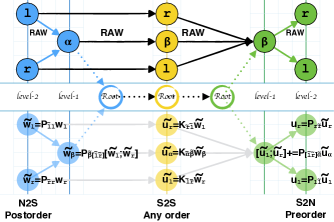
Figure 3. Dependency graph for steps 1–3 of Algorithm 2.7 (step 4 is completely independent of steps 1–3). Each tree node denotes a task, and the arrows between nodes imply a dependency. Here $\mathtt{Near}(\alpha)$ only contains itself (HSS). For example, yellow node $\beta$ has a RAW dependency following blue $\alpha$, because S2S($\beta$) computes ${\widetilde{u}}_{\beta}=\sum_{\alpha\in\mathtt{Near}(\beta)}K_{{\widetilde{\beta}}{\widetilde{\alpha}}}{\widetilde{w}}_{\alpha}$. When $\mathtt{Near}(\beta)$ contains more than just itself. The dependencies are unknown at compile time and thus, omp task depend fails to describe the dependencies between N2S and S2S.

Dependency analysis. Recursive preorder and postorder traversals inherently encode Read/Write dependencies between tree nodes. Following Algorithm 2.2 and Algorithm 2.7, we can describe dependencies between different tasks. However, due to dynamic granularity of tasks we need a data flow analysis at runtime. For example, dependencies between N2S and S2S cannot be discovered at compile time, because the RAW (read after write) dependencies on ${\widetilde{w}}_{\alpha}$ are computed by neighbors ${\mathcal{N}}(\alpha)$. In order to build dependencies at runtime as a direct acyclic graph (DAG), we perform a symbolic execution on Algorithm 2.2 and Algorithm 2.7. For simplicity, below we just discuss the evaluation phase for the HSS case (the FMM case is more involved).

Figure 3 depicts task dependencies (by tasks we mean algorithmic tasks defined in Table 2) during the evaluation phase Algorithm 2.7 for N2S, S2S and S2N where the off-diagonal blocks are low-rank (HSS) with $S=0$. This task dependency tree is generated by our runtime using symbolic traversals. The N2S, S2S, and S2N execution order is performed on a binary tree.

We use three symbolic traversals of Algorithm 2.7. In the first traversal (postorder) we find that ${\widetilde{w}}_{{\tt l}}$ is written by ${\tt l}$. Going from ${\widetilde{w}}_{{\tt l}}$ to ${\widetilde{w}}_{\beta}$, we annotate that ${\widetilde{w}}_{{\tt l}}$ is read by $\beta$, i.e. ${\widetilde{w}}_{\beta}=P_{{\widetilde{\beta}}[{\widetilde{{\tt l}}}{\widetilde{{\tt r}}}]}[{\widetilde{w}}_{{\tt l}};{\widetilde{w}}_{{\tt r}}]$. This RAW dependency is an edge from ${\tt l}$ to $\beta$ in the DAG.

Intertask dependencies are discovered by the symbolic execution of the yellow tree. At node $\beta$ (in yellow), the relation ${\widetilde{u}}_{\alpha}=K_{{\widetilde{\alpha}}{\widetilde{\beta}}{\widetilde{w}}_{\beta}}$ will read ${\widetilde{w_{\beta}}}$. Again this is a RAW dependency, hence the edge from the blue $\beta$ to the yellow $\alpha$. The whole dependency graph for steps 1–3 is built after the green postorder tree traversal. Step 4 in Algorithm 2.7 is independent of steps 1–3. Although this runtime data flow analysis has some overhead, the amount is almost negligible ($<1\%$) compared to the total execution time.

Runtime. With a dependency graph, scheduling can be done in static or dynamic fashion. Due to unknown adaptive rank $s$ at compile time, we implement a light-weight dynamic Heterogeneous Earliest Finish Time (HEFT) (Topcuoglu et al., 2002) using OpenMP threads. Each worker (thread) in the runtime can use more than one physical core with either a nested OpenMP construct or by employing a device (accelerator) as a slave. Tasks that satisfy all dependencies in the DAG will be dispatched to a “ready” queue. Each worker keeps consuming tasks in its own queue until no tasks are left.

Although we estimate a cost for each task in Table 2, the runtime of a normal worker (or one with an accelerator) depends on the problem and can only be determined at runtime. The HEFT schedule is implemented using an estimated finish time of all pending tasks in a specific worker’s ready queue. Each task dispatched from the DAG is assigned to a queue such that the maximum estimated finish time of each queue is minimized. For the case where the estimation is inaccurate, we also implement a job stealing mechanism.

Other parallel implementation. We briefly introduce other possible parallel implementations and conduct a strong scaling experiment in §4. Here we implemented parallel level-by-level traversals for all tasks that require preorder and postorder traversals and do not exploit out-of-order parallelism. For tasks that can be executed in any order, we simply use omp parallel for with dynamic scheduling. If there are not enough tree nodes in a tree level, we use nested parallelism with inner OpenMP constructs and multi-threaded BLAS/LAPACK.

The omp task version is implemented using recursive preorder or postorder traversals. Due to the overhead of the deep call stack, this implementation can be much slower than others. Although we tested it we do not report results because it is not competitive.

We also implemented (and report results for) omp task depend, since OpenMP-4.5 supports task parallelism with dependencies. However there are two issues. First, omp task depend requires all dependencies to be known at compile time, which is not the case for the FMM (tasks N2S and S2S). Second, without knowledge of the estimated finish time, the OpenMP scheduler will be suboptimal. Finally for CPU-GPU hybrid architectures, scheduling GPU tasks purely with omp task can be very challenging.

CPU-GPU hybrid. GPUs usually offer high computing capacity, but performance can easily be bounded by the PCI-E bandwidth. Because most computations in Algorithm 2.2 are complex and memory bound, we do not use GPUs for the compression. Instead we only pre-fetch submatrices $K_{\beta\alpha}$ and $K_{{\widetilde{\beta}}{\widetilde{\alpha}}}$ to the device memory to overlap with computations on the host (CPUs). During the evaluation, our runtime will decide–depending on the number of FLOPS– whether to issue a batch of tasks (up to 8) to the GPU in concurrent (using stream). This usually occurs in N2S and S2N where the size of cublasXgemm is bounded by $s$ and $m$. Furthermore, to hide communication time between CPU and GPU, all arguments of the next task in queue are pre-fetched using asynchronous communication for pipelining. Finally, because a worker with a GPU is usually $50\times$ to $100\times$ more capable than others, we disable job stealing balancing for GPU workers. This optimization prevents the GPU from idling.

3. Experimental Setup

We perform experiments on Haswell, KNL, ARM, and NVIDIA GPU architectures with four different setups to examine the accuracy and efficiency of our methods. We demonstrate (1) the robustness and effectiveness of our geometry-oblivious FMM, (2) the scalability of our runtime system against other parallel schemes, (3) the accuracy and cost comparison with other software, and (4) the absolute efficiency (in percentage of peak performance).

Implementation and hardware. Please refer to §5.2 for all configuration in the reproducibility artifact section. Our tests were conducted on TACC’s Lonestar 5, (two 12-core, 2.6GHz, Xeon E5-2690 v3 “Haswell”), TACC’s Stampede 2 (68-core, 1.4GHz, Xeon Phi 7250 “KNL”) and CSCS’s Piz Daint (12-core, 2.3GHz, Xeon E5-2650 v3 and NVIDIA Tesla P100).

Matrices

We generated 22 matrices emulating different problems. K02 is a 2D regularized inverse Laplacian squared, resembling the Hessian operator of a PDE-constrained optimization problem. The Laplacian is discretized using a 5-stencil finite-difference scheme with Dirichlet boundary conditions on a regular grid. K03 has the same setup with the oscillatory Helmholtz operator and 10 points per wave length. K04–K10 are kernel matrices in six dimensions (Gaussians with different bandwidths, narrow and wide; Laplacian Green’s function, polynomial and cosine-similarity). K12–K14 are 2D advection-diffusion operators on a regular grid with highly variable coefficients. K15,K16 are 2D pseudo-spectral advection-diffusion-reaction operators with variable coefficients. K17 is a 3D pseudo-spectral operator with variable coefficients. K18 is the inverse squared Laplacian in 3D with variable coefficients. G01–G05 are the inverse Laplacian of the powersim, poli_large, rgg_n_2_16_s0, denormal, and conf6_0-8x8-30 graphs from UFL.

K02–K03, K12–K14, and K18 resemble inverse covariance matrices and Hessian operators from optimization and uncertainty quantification problems. K04–K10 resemble classical kernel/Green function matrices but in high dimensions. K15–K17 resemble pseudo-spectral operators. G01–G05 ($N=$ 15838, 15575, 65536, 89400, 49152) are graphs for which we do not have geometric information. For K02–K18, we use $N=65536$ if not specified.

Also, we use kernel matrices from machine learning: COVTYPE (100K, 54D, cartographic variables); and HIGGS (500K, 28D, physics) (Lichman, 2013); MNIST (60K, 780D, digit recognition) (Chang and Lin, 2011). For these datasets, we use a Gaussian kernel with bandwidth $h$.

GOFMM supports both double and single precision. All experiments with matrices K02–K18 and G01–G05 are in single precision. The results for COVTYPE, HIGGS, MNIST are in double precision.

Parameter selection and accuracy metrics. We control $m$ (leaf node size), $s$ (maximum rank), $\tau$ (adaptive tolerance), $\kappa$ (number of neighbors), budget (a key paramter for amount of direct evaluations and for switching between HSS and FMM) and partitioning (Kernel, Angle, Lexicographic, geometric, random). We use $m=$256–512; on average this gives good overall time. The adaptive tolerance $\tau$, reflects the error of the subsampled block and may not correspond to the output error $\epsilon_{2}$. Depending on the problem, $\tau$ may misestimate the rank. Similarly, this may occur in HODLR, STRUMPACK and ASKIT. We use $\tau$ between 1E-2 and 1E-7, $s=m$, $k=32$ and $3\%$ budget. To enforce a HSS approximation, we use $0\%$ budget. The Gaussian bandwidth values are taken from (March et al., 2015b) and produce optimal learning rates.

Throughout we use relative error $\epsilon_{2}$ defined as the following

(11) $$\epsilon_{2}=\|{\widetilde{K}}w-Kw\|_{F}/\|Kw\|_{F},\ \mbox{where}\ w\in\mathbb{R}^{N\times r}.$$

This metric requires ${\mathcal{O}}(rN^{2})$ work; to reduce the computational effort we instead sample 100 rows of $K$. In all tables, we use “Comp” and “Eval” to refer the the compression and evaluation time in seconds, and “GFs” to GFLOPS per node.

4. Empirical Results

We label all experiments from #4 to #5 in tables and figures. We perform strong scaling results on a single Haswell and KNL node in Figure 4, comparing different scheduling schemes. In Figure 5, we examine the accuracy of GOFMM for the different matrices; notice that not all 22 matrices admit good hierarchical low-rank structures in the original order (lexicographic). In Figure 6, we compare FMM ($S\neq 0$ in (1)) to HSS ($S=0$) and show an example in which increasing direct evaluations in FMM results in higher accuracy and shorter wall-clock time. In Figure 7, we present a comparison between five permutation schemes; matrix-defined Gram distances work quite well.

For reference, we compare GOFMM to three other codes: HODLR and STRUMPACK ($S=0$ in these codes) in Table 3 and ASKIT (high-$d$ FMM) in Table 4. The two first codes do not permute $K$. ASKIT is similar to GOFMM but uses level-by-level traversals, does not produce a symmetric $\tilde{K}$, and requires points. Finally, we test GOFMM on four different architectures in Table 5; the performance of GOFMM correlates with the performance of BLAS/LAPACK.

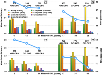
Figure 4. Strong scaling on a single Haswell and KNL node (y-axis, time in seconds on the right, absolute efficiency to the peak GFLOPS on the left). We use $s512$, $\tau 1E-5$ and $r512$. #4 and 4 use COVTYPE to create a Gaussian kernel matrix with $m800$ and $12\%$ budget ($h=0.1$), achieving $\epsilon_{2}=$210-3$$ with average rank $487$. #4 and #4 use K02 with $m512$ and $3\%$ budget, achieving $\epsilon_{2}=$510-5$$ but only with average rank $35$. We increase the number of cores up to 24 Haswell cores and 68 KNL cores. Each set of experiments contains compression time and evaluation time on three different parallel schemes: wall-clock time, level-by-level and omp tasks. We cannot perform scaling experiments for the hybrid CPU-GPU platform (see Table 5 for GPU performance).

Strong scaling (Figure 4). In #1, #2, #3, #4, we use a 24-core Haswell and a 68-core KNL to perform strong scaling experiments. Each set of experiments contains 6 bars including 3 different parallel schemes on both Algorithm 2.2 and Algorithm 2.7. The blue dot indicates the absolute efficiency (ratio to the peak) of our evaluation using dynamic scheduling. #4 and #4 require $12\%$ budget with average rank $487$ to achieve $210-3$. This compute-bound problem can reach $65\%$ peak performance on Haswell and $33\%$ on KNL. However, #4 and #4 only require $3\%$ budget with average rank $35$ to achieve $510-5$. As a result, this memory-bound problem does not scale ($46\%$ and $8\%$) very well. In #4, we can even observe slow down from 34-core to 68-core. This is because the wall-clock time is bounded by the task in the critical path; thus, increasing the number of cores does not help.

Throughout, we can observe that the wall-clock time for compression is less than the level-by-level and omp task traversals. While the work of SKEL is bounded by $2s^{3}$, parallel GEQP3 in the level-by-level traversal does not scale (especially on KNL). On the other hand, task based implementations can execute COEF and Kba out-of-order to maintain the parallelism. Our wall-clock time is better that omp task since we use the cost-estimate model for scheduling.

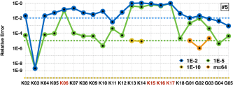
Figure 5. #5, relative error $\epsilon_{2}$ (y-axis, the smaller the better) on all matrices (x-axis) using angle distance. Blue bars use $\tau$110-2$$ and $1\%$ budget (except for K6, K15, K16, K17, other matrices take $0.8$s to compress and $0.1$ to evaluate in average). Green bars use $\tau$110-5$$ and $3\%$ budget (in average, compression takes $1$s and evaluation takes $0.2$s). Red labels denotes matrices that do not compress. K13 and K14 have hierarchical low-rank structure, but the adaptive ID underestimates the rank. K13 and K14 can reach high accuracy (yellow plots) with $\tau$110-10$$ and $3\%$ budget ($1.0$s in compression and $0.2$s in evaluation).

Accuracy (Figure 5). We conduct #5 to examine the accuracy of GOFMM (up to single precision). Given $m512$, $s512$ and $r512$, we report relative error $\epsilon_{2}$ on K02-18 and G01-G05 using the Angle distance with two tolerances: $110-2$ (in blue) and $110-5$ (in green). Throughout, except for K06, K15–K17 (high rank), K13, K14 (underestimating the rank), and G01–G03 (requiring smaller leaf size $m$), other matrices can usually achieve high accuracy with tolerance $110-5$ ($0.9$s in compression and $0.2$s in evaluation). Our adaptive ID underestimates the rank of K13 and K14 such that $\epsilon_{2}$ is high. By imposing a smaller tolerance $110-10$ (yellow plots), both matrices reach $110-5$ ($1$s in compression and $0.2$s in evaluation). K6, K15–K17 have high ranks in the off-diagonal blocks; thus they cannot be compressed with $s512$ and $3\%$ budget. G01–G03 requires direct evaluation in the off-diagonal blocks to reach high accuracy. When we reduce the leaf node size from $512$ to $64$, we can can still reach $110-5$ (orange plots). However, decreasing leaf size to $64$ results in a longer wall-clock time ($0.8s$ in evaluation), because small $m$ hurts performance. Overall, we can observe that GOFMM can quite robustly discover low-rank plus sparse structure from different SPD matrices. We now investigate how increasing the cost (either with higher rank or more direct evaluations) can improve accuracy.

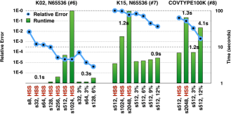
Figure 6. Comparison between HSS and FMM in wall-clock time (seconds, green bars, right y-axis) and accuracy ($\epsilon_{2}$, blue plots, left y-axis). In #6, #6 and #6, we use K02, K15 ($m512$) and COVTYPE ($m800$) datasets. The fixed rank and budget are labeled on x-axis. The green bar is the total wall-clock time including compression and evaluation on $512$ right hand sides. For some experiments, we also provide wall-clock time for evaluation to contrast the trade-off of using high rank and high budget.

Comparison between FMM and HSS (Figure 6). We use #6, #7, and #8 to show that even with more evaluations, FMM can be faster than HSS for the same accuracy. For HSS the relative error in #6 (blue plots) plateaus at $510-4$. Further increasing rank from 256 to 512 (or even 1,024) results in $O(s^{3})$ work (green bars). Using a combination of low-rank ($s64$) and $3\%$ direct evaluation, FMM can achieve higher accuracy with little increment in the evaluation time (compression time remains the same). Similarly, in #6 we can observe that by using $s512$ and $3\%$ budget we achieve better accuracy than the HSS approximation ($s2048$) in less time.

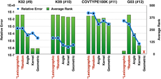
Figure 7. Accuracy (left y-axis) and rank (right, x-axis) comparison: Lexicographic, Random, Kernel 2-norm, Angle and Geometric. We use $\tau$110-7$$, $s512$, $m64$. For methods that define distance, we use $k32$ and $3\%$ budget. G03 is a graph Laplacian; thus, using Geometric distance is impossible.

Permutations (Figure 7). Here we test different permutations (#9, #10, #11, and #12) to discuss the different distances in GOFMM. In each set of experiments, we present relative error (blue plots) and average rank (green bars) for five different schemes. The first two schemes use lexicographic or random order to recursively permute $K$. Since there is no distance defined, these two schemes can only use HSS approximation. The Angle and Kernel distance use the corresponding Gram distances §2.1. Finally, we also use standard geometric distance from points. For the last three schemes, we use $\kappa 32$ and $3\%$ budget. Overall, we can observe that the distance metric is important in discovering low-rank structure and improving accuracy. For example, in #7, Kernel and Geometric show much lower average rank than others. In #7 and #7, although the average ranks are not significantly different, distance-based methods usually have higher accuracy. Finally, we observe for matrix G03 in #7 where no coordinate information exists, our geometry-oblivious methods can still compress the matrix. Although the lexicographic permutation has very low rank, the error is large. This is because the uniform samples for the low-rank approximation are poor. Angle and Kernel distance use neighbors for importantance sampling, which greatly improves the quality of the low-rank approximation.

		HODLR			STRUMPACK			GOFMM
#	case	$\epsilon_{2}$	Comp	Eval	$\epsilon_{2}$	Comp	Eval	$\epsilon_{2}$	Comp	Eval
13	K02	$6.263\,0210-05$	$0.62$	$2.74$	$0.000\,112\,964$	$9.177$	$0.559$	$1.523\,28110-05$	$1.0$	$0.275\,162$
14	K04	$6.400\,2710-05$	$0.67$	$2.69$	$0.000\,120\,927$	$507.754$	$7.8344$	$1.810\,21710-05$	$0.994$	$0.51$
15	K07	$7.262\,2410-05$	$0.87$	$3.06$	$0.000\,227\,985$	$528.377$	$8.202\,18$	$3.933\,85410-05$	$0.588$	$0.240$
16	K12	$6.133\,0610-05$	$0.67$	$2.65$	$0.000\,196\,841$	$18.79$	$0.75$	$1.159\,22710-04$	$0.6$	$0.220$
17	K17	$0.100\,087$	$862.16$	$37.59$	$0.172\,307$	$663.399$	$8.177\,84$	$9.440\,62210-02$	$48.8$	$3.139$
18	G03	$0.000\,270\,227$	$12.92$	$9.67$	$0.025\,486\,9$	$29.7846$	$1.3314$	$8.233\,80810-05$	$0.5$	$0.786$

Table 3. Wall-clock time comparison (in seconds) between HODLR, STRUMPACK, and GOFMM. For K02–K12, we use $N=36K$. K17 uses $N=32K$, and G03 uses $N=65K$. For all software, we use leaf node size $m512$ and $1024$ right hand sides. We control other parameters ($\tau$ and $s$) for each software to target the same relative error ($110-4$).

	Parameters			ASKIT			GOFMM
#	case	$N$	$\tau$	$\epsilon_{2}$	Comp	Eval	$\epsilon_{2}$	Comp	Eval
19	K04	$36\,864$	$110-03$	$0.000\,184\,409$	$0.2878$	$0.021\,256$	$2.362\,88010-04$	$0.5908$	$1.78210-02$
20	K04	$36\,864$	$110-06$	$7.516\,9310-07$	$1.437\,439\,2$	$0.038\,890\,8$	$6.715\,13710-07$	$0.9557$	$2.51610-02$
21	K04	$65\,536$	$110-03$	$0.000\,206\,65$	$1.013\,103$	$0.043\,227$	$1.804\,78210-04$	$1.1819$	$4.21710-02$
22	K04	$65\,536$	$110-06$	$7.359\,5410-07$	$2.238\,445\,9$	$0.083\,464\,1$	$6.132\,38710-07$	$1.6681$	$4.40310-02$
23	K06	$36\,864$	$110-03$	$0.035\,175\,6$	$6.556\,525$	$0.058\,805$	$3.428\,37110-02$	$3.3116$	$3.93910-02$
24	K06	$36\,864$	$110-06$	$0.021\,151\,9$	$7.416\,963\,1$	$0.056\,356\,9$	$3.155\,04410-02$	$4.7576$	$4.68310-02$
25	K06	$65\,536$	$110-03$	$0.038\,055\,4$	$11.056\,666$	$0.109\,234$	$4.461\,60510-02$	$5.6683$	$8.11910-02$
26	K06	$65\,536$	$110-06$	$0.049\,949\,1$	$11.972\,589$	$0.119\,011$	$4.116\,93910-02$	$7.7440$	$8.55410-02$

Table 4. Wall-clock time (in seconds) and accuracy $\epsilon_{2}$ comparison with ASKIT. For both methods, we use $\kappa=32$, $m=s=512$ and $r1$. ASKIT use the $\tau$ reported in the table, and we adjust the tolerance of GOFMM to match the accuracy. For all experiments, GOFMM uses $7\%$ budget. The amount of direct evaluation performed by ASKIT is decided by $\kappa$.

Comparison to existing software (Table 3, Table 4). We compare our methods to HODLR (Ambikasaran and Darve, 2013), STRUMPACK (Rouet et al., 2016), and ASKIT (March et al., 2016). Let us summarize some key differences. HODLR uses the Adaptive Cross Approximation (ACA, partial pivoted LU) for constructing the low-rank blocks (using the Eigen library). Its evaluation requires $O(N\log{N})$ work since the $U$, $V$ matrices are not nested. STRUMPACK constructs an HSS representation in $O(N\log{N})$ work. This is done by using a randomized ID according to (Liberty et al., 2007). We used their black-box compression routine with a uniform random distribution and a Householder rank-revealing QR. Once the matrix is compressed, the evaluation time is $O(N)$ per right hand side. STRUMPACK supports multiple right hand sides. ASKIT’s FMM evaluation has similar complexity as GOFMM, but the amount of direct evaluation is only decided by $\kappa$. For GOFMM, we further introduce the budget to restrict the cost. For all comparisons, we try to match the accuracy by controlling different parameters ($\tau$, $s$, and $\kappa$). Notice that ASKIT and STRUMPACK support MPI, whereas GOFMM does not. We have not used MPI for distributed environment in our experiments.

In Table 3, we target final accuracy $\epsilon_{2}=$110-4$$. GOFMM uses Angle distance for neighbor search and tree partitioning. HODLR and STRUMPACK do not have built-in partitioning schemes for dense matrices. STRUMPACK fails to compress K04 (Gaussian kernel in 6D) and K07 (Laplace kernel in 6D). The first two ones, this is because the lexicographic order does not admit a good $\mathcal{H}\!$-matrix approximation. The matrix needs to be permuted. K17 is difficult to compress with a pure hierarchical low-rank matrix. Finally, G03 performs better when $S\neq 0$. HODLR and STRUMPACK must increase the off-diagonal ranks to match the accuracy and thus the cost increases. GOFMM just uses $S$ and it is about $25\times$ faster in compression and about $1.5\times$ faster in evaluation.

In Table 4, we compare GOFMM (with geometric distances) to ASKIT. ASKIT uses level-by-level traversals in both compression and evaluation. Since ASKIT only evaluates a single right hand side, we use $r=1$. The compression time is inconclusive for #4–#4; the average ranks used in two methods are quite different. The benefit of out-of-order traversal appears in #4–#4 where both methods reach the maximum rank $s$. The speedup in evaluation is not significant. GOFMM can get up to $2\times$ speedup in compression.

#	Arch	Budget	$\epsilon_{2}$	Comp	GFs	Eval	GFs
MNIST60K, $h1$, $\kappa 32$, $m512$, $s128$, $r256$
27	ARM	$5\%$	5E-3	285	3	520	12
COVTYPE100K, $h1$, $\kappa 32$, $m512$, $s128$, $r256$
28	ARM	$5\%$	8E-4	71	2	61	10
COVTYPE100K, $h0.1$, $\kappa 32$, $m800$, $s512$, $r512$
29	CPU	$12\%$	2E-3	30	30	4.1	679
30	CPU$+$GPU	$12\%$	3E-3	33	29	1.7	1952
31	KNL	$12\%$	2E-3	48	25	3.2	1125
HIGGS500K, $h0.9$, $\kappa 64$, $m1024$, $s256$, $r512$
32	CPU	$0.3\%$	2E-1	102	18	3.3	592
33	CPU$+$GPU	$0.3\%$	2E-1	180	12	1.7	1147
34	KNL	$0.3\%$	2E-1	121	17	2.2	872
K02, $N65536$, $\kappa 32$, $m512$, $s512$, $r512$
35	CPU	$3\%$	9E-5	1	25	0.2	889
36	CPU$+$GPU	$3\%$	1E-4	2	12	0.1	2175
37	KNL	$3\%$	1E-4	3	11	0.3	530
K15, $N65536$, $\kappa 32$, $m512$, $s512$, $r1024$
38	CPU	$10\%$	2E-1	6.0	81	1.1	1495
39	CPU$+$GPU	$10\%$	2E-1	7.8	62	0.66	2514
40	KNL	$10\%$	2E-1	9.2	53	1.3	1549
G03, $N65536$, $\kappa 32$, $m128$, $s512$, $r512$
41	CPU	$3\%$	4E-5	4.8	37	0.5	1122
42	CPU$+$GPU	$3\%$	3E-5	7.9	19	0.53	962
43	KNL	$3\%$	5E-5	11.8	9.1	0.6	741
G04, $N89400$, $\kappa 32$, $m512$, $s512$, $r512$
44	CPU	$3\%$	4E-6	1.8	21	0.3	787
45	CPU$+$GPU	$3\%$	4E-6	4.0	10	0.13	2277
46	KNL	$3\%$	4E-6	4.2	9	1.5	215

Table 5. Accuracy $\epsilon_{2}$, wall-clock time (in seconds) and efficiency (in GFLOPS) on four architectures. Because our ARM platform only has a 8GB SD card and 2GB DRAM, we only perform kernel matrices ($K_{ij}$ computed on the fly) with small $r$ and $s$. Note that in the CPU$+$GPU experiment, the compression is run on the CPU (see  §2.3).

Different architectures. In Table 5, we present wall-clock time and GFLOPS of GOFMM on four architectures for different problems. We want to show that the efficiency of GOFMM is portable and only relies on BLAS/LAPACK libraries.

In #5 and #5, we show that a quad-core ARM processor can handle up to 100K fast matrix-multiplication. Because we only have limited memory (2GB) and storage (8GB), in GOFMM we compute $K_{ij}$ on the fly (in detail, we compute $K_{\beta\alpha}$ with a GEMM using the 2-norm expansion). #5 takes much longer than #5 because the cost of evaluating $K_{ij}$ is proportional to the point dimensions of the dataset (MNIST in 780D and COVTYPE in 54D). Because there is no active cooling, the ARM gets overheated and is forced to reduce its clockrate. That is why we can only reach $30\%$ of peak during the evaluation.

Experiments #5 to #5 are computed in double precision. With $12\%$ budget, our evaluation can reach $68\%$ peak performance on Haswell, $37\%$ on KNL and $38\%$ on a hybrid Haswell-P100 system. The performance degrades in #5–5 because the rank is limited to 256, and $0.3\%$ direct evaluation is not enough to create large GEMM calls. For kernel matrices, the GFLOPS for compression are usually higher because computing $K_{ij}$ requires floating point operations. For example, compression of COVTYPE (in 54D) has higher GFLOPS than HIGGS (in 28D). This is not only because COVTYPE is a dataset with high dimensionality, but we also use a higher rank $s512$ such that GEQP3 and TRSM can be more efficient.

Finally, we present performance results on several matrices (#5–5) in single precision. With $10\%$ budget in K15, our evaluation can reach $75\%$ peak on Haswell, $25\%$ on KNL and $25\%$ on a hybrid Haswell-P100 system. This performance requires large leaf node size $m$ and sufficient direct evaluations (e.g. #5–#5). Since G03 requires small $m$, our GFLOPS efficiency degrades due to the dependency on the BLAS/LAPACK routines. Notice that $m128$ is not large enough for GEMM to reach high performance on KNL and GPUs. For G04, we use $m512$ but KNL (#5) does not perform very well. The same problem occurs in Figure 4: the average rank in G04 is too small. Additionally, we do not observe huge performance degradation on GPUs (#5). This is because we enforce our scheduler to schedule L2L tasks to the GPU; thus, tasks with small ranks (N2S and S2N) are mostly consumed by the host CPU. The comparison between #5 and #5 is a good example that highlights the goal of heterogeneous parallel architectures. CPUs with short vector lengths are suitable for tasks with very low ranks (N2S and S2N). On the contrary, GPUs are the method of choice for FLOPS intensive tasks (L2L). We cannot solve such problems with only one architecture efficiently.

5. Conclusions

By using the Gramian vector space for SPD matrices, we defined distances between rows of $K$ using only matrix values. Using the distances, we introduced GOFMM and $\mathcal{H}\!$-matrix scheme that can be used to compress arbitrary SPD matrices (but without accuracy guarantees). In GOFMM we use a shared-memory runtime system that performs out-of-order scheduling in parallel to resolve the dynamic workload due to adaptive ranks and the parallelism-diminishing issue during tree traversals. Our future work will focus on the distributed algorithms and the hierarchical matrix factorization based on our method. We also plan to improve the sampling and pruning quality and to reduce the number of parameters that users need to provide.

Appendix

5.1. Abstract

This artifact description appendix comprises the source code, datasets and installation instruction on a GitHub repository that will be open source and used to reproduce results for our SC’17 paper. We also provide all hardware and software configuration in §5.2. Due to the double-blind peer reviewing policy, we can only provide the url to the repository upon the acceptance.

5.2. Description

Check-list. We briefly describe all meta information. This program implements an algebraic Fast Multipole Method with geometric oblivious technique that generalizes to SPD matrices.

• Program. GOFMM is developed in C++ (with C++11 features) and CUDA, employing OpenMP for shared memory parallelism using a self-contained runtime system.

• Hardware.We conducted experiments on Lonestar5 (two 12-core, 2.6GHz, Xeon E5-2690 v3 “Haswell” per node) and Stampede (68-core, 1.4GHz, Xeon Phi 7250 “KNL” per node) clusters at the Texas Advanced Computing Center, Piz Daint (12-core, 2.3GHz, Xeon E5-2650 v3 and NVIDIA Tesla P100) at Swiss National Supercomputing Centre, and an Intrinsyc Open-Q 820 Development Kit (quad-core, 2.2GHz Qualcomm Kyro).

• Compilation. All software (including HODLR, STRUMPACK and ASKIT) are compiled with intel-16.0 -O3 on Lonestar5 and Piz Daint. Stampede uses intel-17.0 -O3 -xMIC-AVX512. The GPU part uses nvcc-8.0 -O3 -arch$=$sm_60. For Open-Q 820, we cross compile our software with NDK using gcc-4.9 -O3. All CPU and KNL BLAS/LAPACK routines use MKL. GPU BLAS routines use CUBLAS; on ARM we use QSML (Qualcomm Snapdragon Math Library). KNL experiments use Cache-Quadrant configuration. OpenMP uses OMP_PROC_BIND=spread.

• Datasets. Our 22 matrices K02–G05 can be generated using MATLAB scripts (provided in the repo). The urls of the five graphs G01–G05 and the For real world datasets, we provide urls in §3.

• Output. Runtime and total FLOPS of the compression and evaluation phase, accuracy $\epsilon_{2}$ of the first 10 entries and the average of 100 entries.

• Experiment workflow. git clone projects; generate datasets; run test scripts; observe the results;

How delivered. Upon acceptance, we will provide the url to the GOFMM repository on GitHub. The software comprises code, build, and evaluation instructions, and is provided under GPL-3.0 license.

Hardware dependencies. For adequate reproducibility, we suggest that reproducers use the same environment as mentioned above. Notice that we report absolute GFLOPS and the ratio to the peak performance in the paper. For approximately reproducing the same results on a different environment, reproducer should look for platform that has similar capability. The theoretical peak performance in double precision is $998$ GFLOPS per Haswell node, $3,046$ GFLOPS per KNL node, ($4,700+416$) GFLOPS per Tesla P100 node, and $35.2$ GFLOPS per Open-Q820. The peak GFLOPS doubles for single precision computations.

Software dependencies. Compilation requires C/C++ compilers that support c++11 features and OpenMP. GOFMM also requires full functionality of BLAS and LAPACK routines.

5.3. Installation

Given the repository url, you should be able to clone the master branch of the repository. The first step is to edit set_env.sh to select the proper compiler and architecture.

[] export GOFMM_USE_INTEL = true export GOFMM_USE_INTEL = false export GOFMM_USE_CUDA = true export GOFMM_MIC_AVX512= true

If user want to compile the CUDA code for the hybrid CPU-GPU implementation then the following variables have to be exported.

[] export GOFMM_GPU_ARCH_MAJOR=gpu export GOFMM_GPU_ARCH_MINOR=pascal

There are three options for the host (ARM, x86-64 or KNL). Users must choose at least one major and minor architecture to compile. This can be arm/armv8a, x86-64/haswell or mic/knl.

[] export GOFMM_ARCH_MAJOR=arm export GOFMM_ARCH_MINOR=armv8a

export GOFMM_ARCH_MAJOR=x86_64 export GOFMM_ARCH_MINOR=haswell

export GOFMM_ARCH_MAJOR=mic export GOFMM_ARCH_MINOR=knl

Although we use cmake to identify BLAS/LAPACK libraies, but we suggest that user manually setup the path using

[] export GOFMM_QSML_DIR = /path-to-qsml export GOFMM_MKL_DIR = /path-to-mkl export GOFMM_CUDA_DIR = /path-to-cudatoolkit

Finally, users must setup the OpenMP option to enable parallel implementation. Here for example, we use 68 threads for KNL and spread OpenMP thread binding.

[] export OMP_PROC_BIND=spread export OMP_NUM_THREADS=68

With all these options setup, now we use cmake for compilation. Users can use the following commends.

[] source set_env.sh mkdir build cd build cmake .. make make install cd bin ./run_gofmm_x86 ./run_gofmm_gpu ./run_gofmm_knl

Cross compilation. If your ARM runs with OS that has native compiler and cmake support, then the installation instructions above should work just fine. However, while your target runs an Android OS, which currently does not have a native C/C++ compiler, you will need to cross compile this software on your Linux or OSX first. Although there are many ways to do cross compilation, we suggest that users follow these instructions:

• Install Android Studio with LLDB, cmake and NDK support.

• Create stand-alone-toolchain from NDK.

• Install adb (Android Debug Bridge)

• Compile with cmake. It will look for your arm gcc/g++, ar and ranlib support.

• Use the following instructions to push executables and scripts in /build/bin to the Android ARM device.

[] adb devices adb push /build/bin/* /data/local/tmp adb shell cd /data/local/tmp ./run_gofmm_arm.sh

5.4. Dataset

The 22 matrices we use can be generated using MATLAB scripts with the corresponding coordinates or graphs. The five graphs we use in the paper are reported in §3, and the MATLAB scripts will be provided as parts of the source code upon acceptance.

5.5. Experiment workflow

With the repository url, git clone projects. Generate datasets using the provided MATLAB script. Compile GOFMM with the instructions in §5.3. Run the test script for each architecture. Observe the results.

5.6. Evaluation and expected result

For x86-64, ARM and KNL execution, the program will start from the iterative ANN. The accuracy is reported in every iteration. Once the neighbor search is done (or skipped), the metric ball tree partitioning follows. The program reports runtime and total FLOPS of the compression and evaluation phase. Finally, the accuracy $\epsilon_{2}$ is reported in two parts: the error of the first 10 entries, and the average error of 100 entries. Notice that in a CPU-GPU hybrid environment, GOFMM will first try to detect the available GPU device. If successful, the device name and the available global memory size should be displayed. The rest of the execution is the same as our architectures.

References

- (1)
- Agullo et al. (2016) Emmanuel Agullo, Eric Darve, Luc Giraud, and Yuval Harness. 2016. Nearly optimal fast preconditioning of symmetric positive definite matrices. Ph.D. Dissertation. Inria Bordeaux Sud-Ouest.
- Ambikasaran (2013) Sivaram Ambikasaran. 2013. Fast Algorithms for Dense Numerical Linear Algebra and Applications. Ph.D. Dissertation. Stanford University.
- Ambikasaran and Darve (2013) Sivaram Ambikasaran and Eric Darve. 2013. An Fast Direct Solver for Partial Hierarchically Semi-Separable Matrices. Journal of Scientific Computing 57, 3 (2013), 477–501. DOI:https://doi.org/10.1007/s10915-013-9714-z
- Bebendorf (2008) Mario Bebendorf. 2008. Hierarchical matrices. Springer.
- Bebendorf and Rjasanow (2003) Mario Bebendorf and Sergej Rjasanow. 2003. Adaptive low-rank approximation of collocation matrices. Computing 70, 1 (2003), 1–24.
- Benzi et al. (2005) Michele Benzi, Gene H Golub, and Jörg Liesen. 2005. Numerical solution of saddle point problems. Acta numerica 14, 1 (2005), 1–137.
- Cancedda et al. (2003) Nicola Cancedda, Eric Gaussier, Cyril Goutte, and Jean Michel Renders. 2003. Word Sequence Kernels. Journal of Machine Learning Research 3 (March 2003), 1059–1082. http://dl.acm.org/citation.cfm?id=944919.944963
- Chandrasekaran et al. (2010) S. Chandrasekaran, P. Dewilde, M. Gu, and N. Somasunderam. 2010. On the Numerical Rank of the Off-Diagonal Blocks of Schur Complements of Discretized Elliptic PDEs. SIAM J. Matrix Anal. Appl. 31, 5 (2010), 2261–2290. DOI:https://doi.org/10.1137/090775932
- Chang and Lin (2011) Chih-Chung Chang and Chih-Jen Lin. 2011. LIBSVM: A library for support vector machines. ACM Transactions on Intelligent Systems and Technology (TIST) 2, 3 (2011), 27.
- Cheng et al. (1999) H. Cheng, Leslie Greengard, and Vladimir Rokhlin. 1999. A Fast Adaptive Multipole Algorithm in Three Dimensions. J. Comput. Phys. 155 (1999), 468–498.
- Coulier et al. (2016) P. Coulier, H. Pouransari, and E. Darve. 2016. The inverse fast multipole method: using a fast approximate direct solver as a preconditioner for dense linear systems. ArXiv e-prints (2016). arXiv:1508.01835
- Curtin et al. (2013) Ryan R. Curtin, James R. Cline, Neil P. Slagle, William B. March, P. Ram, Nishant A. Mehta, and Alexander G. Gray. 2013. MLPACK: A Scalable C++ Machine Learning Library. Journal of Machine Learning Research 14 (2013), 801–805.
- Dasgupta and Freund (2008) S. Dasgupta and Y. Freund. 2008. Random projection trees and low dimensional manifolds. In Proceedings of the 40th annual ACM symposium on Theory of computing. ACM, 537–546.
- Fong and Darve (2009) William Fong and Eric Darve. 2009. The black-box fast multipole method. J. Comput. Phys. 228, 23 (2009), 8712–8725.
- Ghysels et al. (2016) Pieter Ghysels, Xiaoye S. Li, François-Henry Rouet, Samuel Williams, and Artem Napov. 2016. An Efficient Multicore Implementation of a Novel HSS-Structured Multifrontal Solver Using Randomized Sampling. SIAM Journal on Scientific Computing 38, 5 (2016), S358–S384. DOI:https://doi.org/10.1137/15M1010117
- Grasedyck et al. (2008) Lars Grasedyck, Ronald Kriemann, and Sabine Le Borne. 2008. Parallel black box-LU preconditioning for elliptic boundary value problems. Computing and visualization in science 11, 4 (2008), 273–291.
- Gray and Moore (2001) A.G. Gray and A.W. Moore. 2001. N-body problems in statistical learning. Advances in neural information processing systems (2001), 521–527.
- Greengard et al. (2009) Leslie Greengard, Denis Gueyffier, Per-Gunnar Martinsson, and Vladimir Rokhlin. 2009. Fast direct solvers for integral equations in complex three-dimensional domains. Acta Numerica 18, 1 (2009), 243–275.
- Greengard, L. (1994) Greengard, L. 1994. Fast Algorithms For Classical Physics. Science 265, 5174 (1994), 909–914.
- Hackbusch (2015) Wolfgang Hackbusch. 2015. Hierarchical Matrices: Algorithms and Analysis (1 ed.). Springer-Verlag Berlin Heidelberg.
- Halko et al. (2011) N. Halko, P.-G. Martinsson, and J.A. Tropp. 2011. Finding structure with randomness: Probabilistic algorithms for constructing approximate matrix decompositions. SIAM Rev. 53 (2011), 217–288.
- Ho and Greengard (2012) Kenneth L Ho and Leslie Greengard. 2012. A fast direct solver for structured linear systems by recursive skeletonization. SIAM Journal on Scientific Computing 34, 5 (2012), A2507–A2532.
- Hofmann et al. (2008) Thomas Hofmann, Bernhard Schölkopf, and Alexander J Smola. 2008. Kernel methods in machine learning. The annals of statistics (2008), 1171–1220.
- Karypis and Kumar (1998) George Karypis and Vipin Kumar. 1998. Multilevel -way partitioning scheme for irregular graphs. Journal of Parallel and Distributed computing 48, 1 (1998), 96–129.
- Kondor and Lafferty (2002) Risi Imre Kondor and John Lafferty. 2002. Diffusion kernels on graphs and other discrete input spaces. In ICML, Vol. 2. 315–322.
- Liberty et al. (2007) Edo Liberty, Franco Woolfe, Per-Gunnar Martinsson, Vladimir Rokhlin, and Mark Tygert. 2007. Randomized algorithms for the low-rank approximation of matrices. Proceedings of the National Academy of Sciences 104, 51 (2007), 20167–20172.
- Lichman (2013) M. Lichman. 2013. UCI Machine Learning Repository. (2013). http://archive.ics.uci.edu/ml
- Mahoney and Drineas (2009) M.W. Mahoney and P. Drineas. 2009. CUR matrix decompositions for improved data analysis. Proceedings of the National Academy of Sciences 106, 3 (2009), 697.
- March et al. (2015a) William B. March, Bo Xiao, Sameer Tharakan, Chenhan D. Yu, and George Biros. 2015a. A kernel-independent FMM in general dimensions. In Proceedings of SC15 (The SCxy Conference series). ACM/IEEE, Austin, Texas. http://dx.doi.org/10.1145/2807591.2807647
- March et al. (2015b) William B. March, Bo Xiao, Sameer Tharakan, Chenhan D. Yu, and George Biros. 2015b. Robust treecode approximation for kernel machines. In Proceedings of the 21st ACM SIGKDD Conference on Knowledge Discovery and Data Mining. Sydney, Australia, 1–10. http://dx.doi.org/10.1145/2783258.2783272
- March et al. (2015c) William B. March, Bo Xiao, Chenhan Yu, and George Biros. 2015c. An algebraic parallel treecode in arbitrary dimensions. In Proceedings of IPDPS 2015 (29th IEEE International Parallel and Distributed Computing Symposium). Hyderabad, India. DOI:https://doi.org/10.1109/IPDPS.2015.86
- March et al. (2016) William B. March, Bo Xiao, Chenhan D. Yu, and George Biros. 2016. ASKIT: An Efficient, Parallel Library for High-Dimensional Kernel Summations. SIAM Journal on Scientific Computing 38, 5 (2016), S720–S749. DOI:https://doi.org/10.1137/15M1026468
- Martinsson (2016) Per-Gunnar Martinsson. 2016. Compressing Rank-Structured Matrices via Randomized Sampling. SIAM Journal on Scientific Computing 38, 4 (2016), A1959–A1986. DOI:https://doi.org/10.1137/15M1016679
- Martinsson and Rokhlin (2007) Per-Gunnar Martinsson and Vladimir Rokhlin. 2007. An accelerated kernel-independent fast multipole method in one dimension. SIAM Journal on Scientific Computing 29, 3 (2007), 1160–1178.
- Martinsson et al. (2010) P.-G. Martinsson, V. Rokhlin, and M. Tygert. 2010. A randomized algorithm for the decomposition of matrices. Applied and Computational Harmonic Analysis (2010).
- Muske and Howse (2001) K. R. Muske and J. W. Howse. 2001. A Lagrangian Method for Simultaneous Nonlinear Model Predictive Control. In Large-Scale PDE-constrained Optimization: State-of-the-Art, L.T. Biegler, O. Ghattas, M. Heinkenschloss, and B. van Bloemen Waanders (Eds.). Springer-Verlag.
- Rouet et al. (2016) François-Henry Rouet, Xiaoye S. Li, Pieter Ghysels, and Artem Napov. 2016. A Distributed-Memory Package for Dense Hierarchically Semi-Separable Matrix Computations Using Randomization. ACM Transactions in Mathematical Software 42, 4, Article 27 (June 2016), 35 pages. DOI:https://doi.org/10.1145/2930660
- Schölkopf and Smola (2002) Bernhard Schölkopf and Alexander J Smola. 2002. Learning with kernels: support vector machines, regularization, optimization, and beyond. MIT press.
- Sodani et al. (2016) Avinash Sodani and others. 2016. Knights Landing: Second-Generation Intel Xeon Phi Product. IEEE Micro 36, 2 (2016), 34–46.
- Topcuoglu et al. (2002) Haluk Topcuoglu, Salim Hariri, and Min-you Wu. 2002. Performance-effective and low-complexity task scheduling for heterogeneous computing. IEEE transactions on parallel and distributed systems 13, 3 (2002), 260–274.
- Williams and Seeger (2001) Christopher Williams and Matthias Seeger. 2001. Using the Nyström method to speed up kernel machines. In Proceedings of the 14th Annual Conference on Neural Information Processing Systems. 682–688.
- Xia et al. (2010) Jianlin Xia, Shivkumar Chandrasekaran, Ming Gu, and Xiaoye S Li. 2010. Fast algorithms for hierarchically semiseparable matrices. Numerical Linear Algebra with Applications 17, 6 (2010), 953–976.
- Xiao and Biros (2016) Bo Xiao and George Biros. 2016. Parallel Algorithms for Nearest Neighbor Search Problems in High Dimensions. SIAM Journal on Scientific Computing 38, 5 (2016), S667–S699. DOI:https://doi.org/10.1137/15M1026377
- Ying et al. (2004) Lexing Ying, George Biros, and Denis Zorin. 2004. A kernel-independent adaptive fast multipole method in two and three dimensions. J. Comput. Phys. 196, 2 (2004), 591–626.
- Yokota et al. (2016) Rio Yokota, Huda Ibeid, and David Keyes. 2016. Fast Multipole Method as a Matrix-Free Hierarchical Low-Rank Approximation. Computing Research Repository abs/1602.02244 (2016). http://arxiv.org/abs/1602.02244
- Yu et al. (2015) Chenhan D Yu, Jianyu Huang, Woody Austin, Bo Xiao, and George Biros. 2015. Performance optimization for the k-nearest neighbors kernel on x86 architectures. In Proceedings of the International Conference for High Performance Computing, Networking, Storage and Analysis. ACM, 7.