The converse of the passivity and small-gain theorems for input-output maps

Abstract

We prove the following converse of the passivity theorem. Consider a causal system given by a sum of a linear time-invariant and a passive linear time-varying input-output map. Then, in order to guarantee stability (in the sense of finite $\boldsymbol{\rm L}_{2}$-gain) of the feedback interconnection of the system with an arbitrary nonlinear output strictly passive system, the given system must itself be output strictly passive. The proof is based on the S-procedure lossless theorem. We discuss the importance of this result for the control of systems interacting with an output strictly passive, but otherwise completely unknown, environment. Similarly, we prove the necessity of the small-gain condition for closed-loop stability of certain time-varying systems, extending the well-known necessity result in linear robust control.

1 Introduction

The passivity and small-gain theorems are fundamental to large parts of systems and control theory, see e.g. [13, 9, 12, 7, 11]. Both theorems provide a stability ‘certificate’ when feedback interconnecting the given system with an arbitrary system which is either (in the small-gain setting) assumed to have an $L_{2}$-gain smaller than the reciprocal of the $L_{2}$-gain of the given system, or is (output strictly) passive like the given system. These theorems are valid from linear finite-dimensional systems to nonlinear and infinite-dimensional systems.

The current paper is concerned with the converse of these theorems; that is the necessity of the (strict) passivity or the small-gain condition for closed-loop stability when feedback interconnecting a given system with an arbitrary system, which is unknown apart from a passivity or $\boldsymbol{\rm L}_{2}$-gain assumption. Surprisingly, this converse of the passivity theorem has hardly been studied in the literature; despite its fundamental importance in applications. For example, in order to guarantee stability of a controlled robotic system interacting with a passive, but else completely unknown, environment, the converse of the passivity theorem tells us that the controlled robot must be output strictly passive as seen from the interaction port of the robot with the environment. This has far-reaching methodological implications for control design, since it means that rendering by control the system output strictly passive at the interaction port is not only a valid option, but is the only option guaranteeing stability for an unknown passive environment. The same holds within the context of robust nonlinear control whenever we replace ‘environment’ by the uncertain part of the system.

Up to now this converse passivity theorem was only proved for linear time-invariant single-input single-output systems in [1], using arguments from Nyquist stability theory, exactly with the robotics motivation in mind. The same motivation was elaborated on in [10], where the following form of a converse passivity theorem was obtained for nonlinear systems in state space form. If a system is not passive then for any given constant $K$ one can define a passive system that extracts from the given system an amount of energy that is larger than $K$, implying that the norm of the state of the constructed system becomes larger than $K$, thereby demonstrating some sort of instability of the closed-loop system. In the present paper, a converse of the passivity theorem will be derived for a class of input-output maps, namely those decomposable into a sum of a linear time-invariant map and a passive linear time-varying map. This converse passivity theorem involves feedback interconnections with nonlinear systems and will be formulated in three versions in Section 3, with their own range of applicability. In all cases the proofs are based on the S-procedure lossless theorem due to Megretski & Treil [8]; see also [4, Thm. 7].

Converse statements of the small-gain theorem are much more present in the literature; see e.g. [14, Theorem 9.1] for the finite-dimensional linear case and [2] for infinite-dimensional linear systems. However, to the best of our knowledge, the converse of the small-gain theorem for linear time-varying systems interconnected in feedback with nonlinear systems, as obtained in Section 4, is new, while also the proof line is different from the existing one. Similarly to the passivity case, this converse will be formulated for a class of linear time-varying input-output maps, and the proofs, in two different versions, will be based on the S-procedure lossless theorem.
Finally, Section 5 presents the conclusions, and discusses problems for further research. A preliminary version of some of the results in Section 3 of this paper was presented at the IFAC World Congress 2017; cf. [6].

2 Preliminaries

This section summarizes the background for this paper; see e.g. [11] for details. Denote the set of $\mathbb{R}^{n}$-valued Lebesgue square-integrable functions by

$$\boldsymbol{\rm L}_{2}^{n}:=\Big{\{}v:[0,\infty)\to\mathbb{R}^{n}\mid\|v\|_{2}^{2}:=\int_{0}^{\infty}v(t)^{T}v(t)\,dt<\infty\Big{\}}.$$

For any two $v,w\in\boldsymbol{\rm L}_{2}^{n}$ denote the $\boldsymbol{\rm L}_{2}^{n}$-inner product as

$$\langle v,w\rangle:=\int_{0}^{\infty}v(t)^{T}w(t)\,dt$$

Define the truncation operator $(P_{T}v)(t):=v(t)$ for $t\leq T$; $(P_{T}v)(t):=0$ for $t>T$, and the extended function space

$$\boldsymbol{\rm L}_{2e}^{n} :=\{v:[0,\infty)\to\mathbb{R}^{n}\mid P_{T}v\in\boldsymbol{\rm L}_{2},\;\forall T\in[0,\infty)\}.$$

In what follows, the superscript $n$ will often be suppressed for notational simplicity. Throughout this paper a system will be specified by an input-output map $\Delta:\boldsymbol{\rm L}_{2e}^{m}\to\boldsymbol{\rm L}_{2e}^{p}$ satisfying $\Delta(0)=0$.
Define for any $\tau\geq 0$ the right shift operator $(S_{\tau}(u))(t)=u(t-\tau)$ for $t\geq\tau$ and $(S_{\tau}(u))(t)=0$ for $0\leq t<\tau$. The system $\Delta$ is said to be time-invariant if $S_{\tau}\Delta=\Delta S_{\tau}$ for all $\tau>0$. Furthermore, the system $\Delta$ is bounded if $\Delta$ maps $\boldsymbol{\rm L}_{2}^{m}$ into $\boldsymbol{\rm L}_{2}^{p}$. It is said to have $\boldsymbol{\rm L}_{2}$-gain $\leq\gamma$ for some $\gamma>0$ (finite $\boldsymbol{\rm L}_{2}$-gain) if

$$\|P_{T}\Delta(u)\|_{2}\leq\gamma\|P_{T}u\|_{2}$$ (1)

for all $u\in\boldsymbol{\rm L}_{2e}^{m}$ and all $T\geq 0$. The infimum of all $\gamma$ satisfying (1) is called the $\boldsymbol{\rm L}_{2}$-gain of $\Delta$. The system $\Delta$ is causal if $P_{T}\Delta P_{T}=P_{T}\Delta$ for all $T\geq 0$. It is well-known, see e.g. [11, Proposition 1.2.3], that a causal system $\Delta$ has finite $\boldsymbol{\rm L}_{2}$-gain if and only if, instead of (1),

$$\|\Delta(u)\|_{2}\leq\gamma\|u\|_{2}$$ (2)

for all $u\in\boldsymbol{\rm L}_{2}^{m}$. For the purpose of interconnection of systems the above notions are generalized from maps to relations $R\subset\boldsymbol{\rm L}_{2e}^{m}\times\boldsymbol{\rm L}_{2e}^{p}$ satisfying $(0,0)\in R$ as follows [11]. A relation $R$ is said to be bounded if whenever $(u,y)\in R$ and $u\in\boldsymbol{\rm L}_{2}$ then also $y\in\boldsymbol{\rm L}_{2}$. Furthermore, $R$ has finite $\boldsymbol{\rm L}_{2}$-gain if

$$\|P_{T}y\|_{2}\leq\gamma\|P_{T}u\|_{2}$$ (3)

for all $(u,y)\in R$ and all $T\geq 0$. Also, $R$ is said to be causal if whenever $(u_{1},y_{1})\in R$, $(u_{2},y_{2})\in R$ satisfy $P_{T}u_{1}=P_{T}u_{2}$, then $P_{T}y_{1}=P_{T}y_{2}$. A causal relation $R$ has finite $\boldsymbol{\rm L}_{2}$-gain if and only i,f instead of (3) ,

$$\|y\|_{2}\leq\gamma\|u\|_{2}$$ (4)

for all $\boldsymbol{\rm L}_{2}$ pairs $(u,y)\in R$. The system $\Delta:\boldsymbol{\rm L}_{2e}^{m}\to\boldsymbol{\rm L}_{2e}^{m}$ (i.e., $p=m$) is said to be passive [13, 12] if

$$\int_{0}^{T}u(t)^{T}(\Delta(u))(t)\,dt\geq 0,$$ (5)

for all $u\in\boldsymbol{\rm L}_{2e},T>0$. Furthermore, it is called strictly passive if there exist $\delta>0,\epsilon>0$ such that

$$\int_{0}^{T}u(t)^{T}(\Delta(u))(t)\,dt\geq\delta\|P_{T}u\|_{2}^{2}+\epsilon\|P_{T}\Delta(u)\|_{2}^{2}$$

for all $u\in\boldsymbol{\rm L}_{2e},T>0$, and output strictly passive if this holds with $\delta=0$. In case $\Delta$ is bounded and causal, then passivity is equivalent [11, Proposition 2.2.5] to

$$\int_{0}^{\infty}u(t)^{T}(\Delta(u))(t)\,dt\geq 0$$ (6)

for all $u\in\boldsymbol{\rm L}_{2}^{m}$. (Note that the integral is well-defined because of boundedness of $\Delta$ and the Cauchy-Schwartz inequality.) Similarly, in this case $\Delta$ is strictly passive if there exist $\delta>0,\epsilon>0$ such that

$$\int_{0}^{\infty}u(t)^{T}(\Delta(u))(t)\,dt\geq\delta\|u\|_{2}^{2}+\epsilon\|\Delta(u)\|_{2}^{2}\quad\forall u\in\boldsymbol{\rm L}_{2}^{m},$$ (7)

and output strictly passive if this holds with $\delta=0$. For later use we also recall the basic property that any output strictly passive system has finite $\boldsymbol{\rm L}_{2}$-gain; cf. [11, Theorem 2.2.13]. Like in the $\boldsymbol{\rm L}_{2}$-case these passivity notions are directly extended to relations $R\subset\boldsymbol{\rm L}_{2e}^{m}\times\boldsymbol{\rm L}_{2e}^{m}$ satisfying $(0,0)\in R$. Indeed, $R$ is called strictly passive if there exist $\delta>0,\epsilon>0$ such that for all $(u,y)\in R$, $T>0$

$$\int_{0}^{T}u(t)^{T}y(t)\,dt\geq\delta\|P_{T}u\|_{2}^{2}+\epsilon\|P_{T}y\|_{2}^{2},$$ (8)

and output strictly passive if this holds with $\delta=0$. Furthermore, a bounded causal relation $R$ is strictly passive if there exist $\delta>0,\epsilon>0$ such that for all $(u,y)\in R$

$$\int_{0}^{\infty}u(t)^{T}y(t)\,dt\geq\delta\|u\|_{2}^{2}+\epsilon\|y\|_{2}^{2},$$ (9)

and output strictly passive if this holds with $\delta=0$.

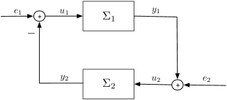
Figure 1: Feedback configuration

The main object of study in this paper is the feedback interconnection of two systems $\Sigma_{1}:\boldsymbol{\rm L}_{2e}^{m_{1}}\to\boldsymbol{\rm L}_{2e}^{p_{1}}$ and $\Sigma_{2}:\boldsymbol{\rm L}_{2e}^{m_{2}}\to\boldsymbol{\rm L}_{2e}^{p_{2}}$, with $m_{1}=p_{2},m_{2}=p_{1}$, described by (see Figure 1)

$$\begin{array}[]{rcllll}u_{1}&=&e_{1}-y_{2},&u_{2}&=&e_{2}+y_{1},\\[5.69054pt] y_{1}&=&\Sigma_{1}(u_{1}),&y_{2}&=&\Sigma_{2}(u_{2}).\end{array}$$ (10)

The resulting closed-loop system with inputs $(e_{1},e_{2})$ and outputs $(y_{1},y_{2})$ will be denoted by $\Sigma_{1}\|\Sigma_{2}$, and defines by (10) a relation in the space of all $(e_{1},e_{2},u_{1},u_{2},y_{1},y_{2})\in\boldsymbol{\rm L}_{2e}$. Projection on the space of $(e_{1},e_{2},u_{1},u_{2})\in\boldsymbol{\rm L}_{2e}$, respectively of $(e_{1},e_{2},y_{1},y_{2})\in\boldsymbol{\rm L}_{2e}$, yields the relations

$$\begin{array}[]{rcl}R_{eu}\!&:=&\!\{(e_{1},e_{2},u_{1},u_{2})\in\boldsymbol{\rm L}_{2e}\!\mid\!\eqref{eq: FB}\mbox{ holds for some }y_{1},y_{2}\}\\[5.69054pt] R_{ey}\!&:=&\!\{(e_{1},e_{2},y_{1},y_{2})\in\boldsymbol{\rm L}_{2e}\!\mid\!\eqref{eq: FB}\mbox{ holds for some }u_{1},u_{2}\}\end{array}$$

Definition 2.1.

The feedback interconnection $\Sigma_{1}\|\Sigma_{2}$ has finite $\boldsymbol{\rm L}_{2}$-gain if the relation $R_{eu}$, or equivalently (see [11, Lemma 1.2.12], the relation $R_{ey}$, has finite $\boldsymbol{\rm L}_{2}$-gain. $\Sigma_{1}\|\Sigma_{2}$ with $m_{1}=m_{2}=p_{1}=p_{2}$ is said to be passive whenever the relation $R_{ey}$ is passive. The feedback interconnection for $e_{2}=0$, denoted by $\Sigma_{1}\|_{e_{2}=0}\Sigma_{2}$, is said to have finite $\boldsymbol{\rm L}_{2}$-gain if the corresponding relation $R_{e_{1}y_{1}}$ has finite $\boldsymbol{\rm L}_{2}$-gain, and is said to be passive if $R_{e_{1}y_{1}}$ is passive. For notational convenience, we denote the map from $e_{1}$ to $y_{1}$ by $\Sigma_{1}\|_{e_{2}=0}\Sigma_{2}$.

Finally, if the systems $\Sigma_{1}$ and $\Sigma_{2}$ are causal, then so are the relations $R_{ey}$ and $R_{eu}$; see [11, Proposition 1.2.14]. The same statement is easily seen to hold for $R_{e_{1}y_{1}}$. All systems and relations are taken to be causal throughout this paper.

3 Passivity as a necessary condition for stable interaction

The classical passivity theorem, see e.g. [11], asserts that the feedback interconnection $\Sigma_{1}\|\Sigma_{2}$ of two passive systems $\Sigma_{1},\Sigma_{2}$ is again a passive system. Similarly, the interconnected system $\Sigma_{1}\|_{e_{2}=0}\Sigma_{2}$ is passive. In this section we will derive a converse passivity theorem stating that a necessary condition in order that any closed-loop system arising from interconnecting a given system $\Sigma_{1}$ to with an unknown, but output strictly passive, system $\Sigma_{2}$ is stable (in the sense of having finite $\boldsymbol{\rm L}_{2}$-gain), is that the system $\Sigma_{1}$ is itself output strictly passive. As already indicated in the introduction, this result is crucial e.g. in the control of robotic systems; see also the discussion and example at the end of this section. We will formulate three different versions of this theorem. Before doing so we first state the following version of the S-procedure lossless theorem, which can be obtained from [4, Thm. 7 and Ex. 28], based on [8].

Proposition 3.1 (S-procedure lossless theorem).

Let $\mathcal{H}\subset\boldsymbol{\rm L}_{2}$ be a vector space satisfying $S_{\tau}\mathcal{H}\subset\mathcal{H}$ for all $\tau\geq 0$ and $\sigma_{i}:\mathcal{H}\to\mathbb{R}$ be defined as $\sigma_{i}(f):=\langle f,\Phi_{i}f\rangle$, where $\Phi_{i}=\Phi_{i}^{T}$ is a constant matrix, $i=0,1$. Suppose there exists an $f^{*}\in\mathcal{H}$ such that $\sigma_{1}(f^{*})>0$, then the following are equivalent:

1. $\sigma_{0}(f)\leq 0$ for all $f\in\mathcal{H}$ such that $\sigma_{1}(f)\geq 0$;

2. $\exists\mu\geq 0$ such that $\sigma_{0}(f)+\mu\sigma_{1}(f)\leq 0,\quad\forall f\in\mathcal{H}$.

The first version of the converse passivity theorem is as follows.

Theorem 3.2.

Given bounded $\Sigma_{1}=G+\Delta$, where $G$ is linear time-invariant and $\Delta$ is linear passive, then there exists $\gamma>0$ such that the closed-loop system $\Sigma_{1}\|\Sigma_{2}$ has $\boldsymbol{\rm L}_{2}$-gain $\leq\gamma$ for all bounded passive $\Sigma_{2}$ if and only if $\Sigma_{1}$ is strictly passive.

Proof   Sufficiency is well known in the literature. Indeed, strict passivity of $\Sigma_{1}$ together with passivity of $\Sigma_{2}$ yields

$$\epsilon(\|y_{1}\|_{2}^{2}+\|u_{1}\|_{2}^{2}) \leq\langle u_{1},y_{1}\rangle+\langle u_{2},y_{2}\rangle$$

$$=\langle e_{1}-y_{2},y_{1}\rangle+\langle e_{2}+y_{1},y_{2}\rangle$$

$$=\langle e_{1},y_{1}\rangle+\langle e_{2},y_{2}\rangle.$$

Therefore, substituting $u_{1}=e_{1}-y_{2},u_{2}=e_{2}+y_{1}$,

$$\|y_{1}\|_{2}^{2}+\langle e_{1}-y_{2},e_{1}-y_{2}\rangle\leq\frac{1}{\epsilon}(\langle e_{1},y_{1}\rangle+\langle e_{2},y_{2}\rangle),$$

or

$$\|y_{1}\|_{2}^{2}+\|y_{2}\|_{2}^{2}-2\langle e_{1},y_{2}\rangle+\|e_{1}\|_{2}^{2}\leq\frac{1}{\epsilon}(\langle e_{1},y_{1}\rangle+\langle e_{2},y_{2}\rangle).$$

It follows that

$$\|y\|_{2}^{2}\leq 2\langle e_{1},y_{2}\rangle+\frac{1}{\epsilon}\langle e,y\rangle\leq\left(2+\frac{1}{\epsilon}\right)\|e\|_{2}\|y\|_{2},$$

where $y:=(y_{1},y_{2})^{T}$ and $e:=(e_{1},e_{2})^{T}$, and the Cauchy-Schwarz inequality has been used. Dividing both sides by $\|y\|_{2}$ the result follows.
To show necessity, let $\tilde{G}_{\epsilon}:=G-\epsilon I$ and $\tilde{\Delta}_{\epsilon}:=\Delta+\epsilon I$ for $\epsilon>0$ so that $\Sigma_{1}=\tilde{G}_{\epsilon}+\tilde{\Delta}_{\epsilon}$. Recall from the theory of loop transformations [3, Section 3.5] that the finite $\boldsymbol{\rm L}_{2}$-gain of $\Sigma_{1}\|\Sigma_{2}$ is equivalent to that of $\tilde{G}_{\epsilon}\|[\Sigma_{2}\|_{e_{2}=0}\tilde{\Delta}_{\epsilon}]$. Furthermore, since $\tilde{\Delta}_{\epsilon}$ is strictly passive, that $\tilde{G}_{\epsilon}\|[\Sigma_{2}\|_{e_{2}=0}\tilde{\Delta}_{\epsilon}]$ has $\boldsymbol{\rm L}_{2}$-gain $\leq\gamma$ for all bounded passive $\Sigma_{2}$ and $\epsilon>0$ is equivalent to $G\|\Sigma_{2}$ having $\boldsymbol{\rm L}_{2}$-gain $\leq\gamma$ for all bounded passive $\Sigma_{2}$. Define the vector space

$$\mathcal{H}:=\{(u_{1},u_{2},e_{1},e_{2})\in\boldsymbol{\rm L}_{2}\ |\ u_{2}=e_{2}+G(u_{1})\}.$$

Note that $S_{\tau}\mathcal{H}\subset\mathcal{H}$ for all $\tau\geq 0$ due to the time-invariance of $G$. Define now the following quadratic forms $\sigma_{i}:\mathcal{H}\to\mathbb{R}$, $i=0,1$, as

$$\sigma_{0}(u_{1},u_{2},e_{1},e_{2}) :=\left\langle\begin{bmatrix}u_{1}\\ u_{2}\\ e_{1}\\ e_{2}\end{bmatrix},\begin{bmatrix}I&0&0&0\\ 0&I&0&0\\ 0&0&-\gamma^{2}I&0\\ 0&0&0&-\gamma^{2}I\end{bmatrix}\begin{bmatrix}u_{1}\\ u_{2}\\ e_{1}\\ e_{2}\end{bmatrix}\right\rangle$$

$$\sigma_{1}(u_{1},u_{2},e_{1},e_{2}) :=\frac{1}{2}\left\langle\begin{bmatrix}u_{1}\\ u_{2}\\ e_{1}\\ e_{2}\end{bmatrix},\begin{bmatrix}0&-I&0&0\\ -I&0&I&0\\ 0&I&0&0\\ 0&0&0&0\end{bmatrix}\begin{bmatrix}u_{1}\\ u_{2}\\ e_{1}\\ e_{2}\end{bmatrix}\right\rangle.$$

Note that $\sigma_{1}(u_{1},u_{2},e_{1},e_{2})=u_{2}^{T}(e_{1}-u_{1})$, and hence it is easy to see that there exists $(u_{1}^{*},u_{2}^{*},e_{1}^{*},e_{2}^{*})\in\mathcal{H}$ such that $\sigma_{1}(u_{1}^{*},u_{2}^{*},e_{1}^{*},e_{2}^{*})>0$. It is immediately seen that $\sigma_{0}\leq 0$ corresponds to the $\boldsymbol{\rm L}_{2}$-gain of $R_{eu}$ being $\leq\gamma$, while $\sigma_{1}\geq 0$ corresponds to any bounded passive $\Sigma_{2}$. Hence, if the closed-loop system $G\|\Sigma_{2}$ has $\boldsymbol{\rm L}_{2}$-gain $\leq\gamma$ for all bounded passive $\Sigma_{2}$, then

$$\sigma_{0}(u_{1},u_{2},e_{1},e_{2})\leq 0\quad\forall (u_{1},u_{2},e_{1},e_{2})\in\mathcal{H}$$

$$\text{such that}\;\sigma_{1}(u_{1},u_{2},e_{1},e_{2})\geq 0.$$

This is equivalent, via the S-procedure lossless theorem (cf. Proposition 3.1), to the existence of $\mu\geq 0$ such that

$$\sigma_{0}(u_{1},u_{2},e_{1},e_{2})+\mu\sigma_{1}(u_{1},u_{2}, e_{1},e_{2})\leq 0,$$

$$\forall(u_{1},u_{2},e_{1},e_{2})\in\mathcal{H}.$$

Within the subset $\{(u_{1},u_{2},0,0)\in\boldsymbol{\rm L}_{2}\ |\ u_{2}=G(u_{1})\}\subset\mathcal{H}$, this yields

$$\|G(u_{1})\|_{2}^{2}+\|u_{1}\|_{2}^{2}-\mu\langle u_{1},G(u_{1})\rangle\leq 0,\quad\forall u_{1}\in\boldsymbol{\rm L}_{2}.$$

This implies $\mu>0$, and thus

$$\langle u_{1},G(u_{1})\rangle\geq\frac{1}{\mu}(\|G(u_{1})\|_{2}^{2}+\|u_{1}\|_{2}^{2}),\quad\forall u_{1}\in\boldsymbol{\rm L}_{2},$$

i.e., $G$ is strictly passive. Consequently, $\Sigma_{1}$ is strictly passive.

Roughly speaking, the new ‘only if’ direction of the above theorem can be summarized by saying that in order that $\Sigma_{1}\|\Sigma_{2}$ is stable (in the sense of having uniformly bounded $\boldsymbol{\rm L}_{2}$-gain) for all passive $\Sigma_{2}$, then $\Sigma_{1}$ needs to be strictly passive. On the other hand, often in physical system examples (e.g., most mechanical systems) output strict passivity is a more natural property, since strict passivity can only occur for systems with direct feedthrough term; see [11, Proposition 4.1.2]. The following second version of the converse passivity theorem obviates this problem.

Figure 2: Loop transformation

Theorem 3.3.

Given bounded $\widetilde{\Sigma}_{1}=G+\Delta$, where $G$ is linear time-invariant and $\Delta$ is linear passive, then there exists $\gamma>0$ such that the closed-loop system $\widetilde{\Sigma}_{1}\|\widetilde{\Sigma}_{2}$ has $\boldsymbol{\rm L}_{2}$-gain $\leq\gamma$ for all output strictly passive $\widetilde{\Sigma}_{2}$ if and only if $\widetilde{\Sigma}_{1}$ is output strictly passive.

Proof   Sufficiency can be shown in a similar manner using the arguments in the sufficiency proof for Theorem 3.2; see also [11]. For necessity, note that for any $\epsilon>0$ the output strictly passive $\widetilde{\Sigma}_{2}$ can be written as the feedback interconnection of a bounded passive $\Sigma_{2}$ and $\epsilon I$, where $I$ denotes the identity operator. To see this, define $\Sigma_{2}$ as in Figure 2. Then by output strict passivity of $\widetilde{\Sigma}_{2}$

$$\int_{0}^{\infty}\tilde{u}_{2}(t)^{T}y_{2}(t)\,dt\geq\epsilon\|y_{2}\|_{2}^{2}\quad\forall\tilde{u}_{2}\in\boldsymbol{\rm L}_{2},$$

implying that

$$\int_{0}^{\infty}(\tilde{u}_{2}(t)-\epsilon y_{2}(t))^{T}y_{2}(t)\,dt=\int_{0}^{\infty}u_{2}(t)^{T}y_{2}(t)\,dt\geq 0.$$

The last inequality holds for all $u_{2}\in\boldsymbol{\rm L}_{2}$, since given any $u_{2}\in\boldsymbol{\rm L}_{2}$, $\tilde{u}_{2}:=(I+\epsilon\Sigma_{2})u_{2}\in\boldsymbol{\rm L}_{2}$ yields the desired $u_{2}$. It follows that $\Sigma_{2}$ is bounded and passive. By the same token, the negative feedback interconnection of a bounded passive $\Sigma_{2}$ and $\epsilon I$ with $\epsilon>0$ is output strictly passive. By defining $\Sigma_{1}:=\widetilde{\Sigma}_{1}+\epsilon I$ as illustrated in Figure 2, one obtains the loop transformation configuration therein. Since finite $\boldsymbol{\rm L}_{2}$-gain of the closed-loop system $\widetilde{\Sigma}_{1}\|\widetilde{\Sigma}_{2}$ in Figure 2 is equivalent to that of $\Sigma_{1}\|\Sigma_{2}$ in Figure 1 [3, Section 3.5], application of Theorem 3.2 then yields that $\Sigma_{1}$ is strictly passive. For sufficiently small $\epsilon>0$, it follows that $\widetilde{\Sigma}_{1}=\Sigma_{1}-\epsilon I$ is output strictly passive.

Both Theorems 3.2 and 3.3 require an exogenous signal $e_{2}$, which is often not the typical case in applications. This motivates the following third version of the converse passivity theorem.

Theorem 3.4.

Given bounded $\Sigma_{1}=G+\Delta$, where $G$ is linear time-invariant and $\Delta$ is linear passive, then there exists $\gamma>0$ such that the closed-loop system $\Sigma_{1}\|_{e_{2}=0}\Sigma_{2}$ has $\boldsymbol{\rm L}_{2}$-gain from $e_{1}$ to $y_{1}$ less than or equal to $\gamma$ for all bounded passive $\Sigma_{2}$ if and only if $\Sigma_{1}$ is output strictly passive.

Proof   Sufficiency is well known in the literature. Indeed, if $\Sigma_{1}$ is output strictly passive and $\Sigma_{2}$ is passive, then for some $\varepsilon>0$

$$\langle e_{1},y_{1}\rangle =\langle u_{1}+y_{2},y_{1}\rangle=\langle u_{1},y_{1}\rangle+\langle y_{2},y_{1}\rangle$$

$$=\langle u_{1},y_{1}\rangle+\langle u_{2},y_{2}\rangle\geq\varepsilon\|y_{1}\|_{2}^{2},$$

showing that the closed-loop system is $\varepsilon$-output strictly passive, and hence (see e.g. [11], Theorem 2.2.13) has $\boldsymbol{\rm L}_{2}$-gain $\leq\frac{1}{\varepsilon}$. To show necessity, note that by the same arguments in Theorem 3.2, the hypothesis is equivalent to $G\|_{e_{2}=0}\Sigma_{2}$ having $\boldsymbol{\rm L}_{2}$-gain $\leq\gamma$ for all bounded passive $\Sigma_{2}$. Define

$$\mathcal{H}:=\{(u_{1},y_{1},e_{1})\in\boldsymbol{\rm L}_{2}\ |\ y_{1}=G(u_{1})\}$$

and the quadratic forms $\sigma_{i}:\mathcal{H}\to\mathbb{R}$, $i=0,1$, as

$$\sigma_{0}(u_{1},y_{1},e_{1}) :=\left\langle\begin{bmatrix}u_{1}\\ y_{1}\\ e_{1}\end{bmatrix},\begin{bmatrix}0&0&0\\ 0&I&0\\ 0&0&-\gamma^{2}I\end{bmatrix}\begin{bmatrix}u_{1}\\ y_{1}\\ e_{1}\end{bmatrix}\right\rangle$$

$$\sigma_{1}(u_{1},y_{1},e_{1}) :=\frac{1}{2}\left\langle\begin{bmatrix}u_{1}\\ y_{1}\\ e_{1}\end{bmatrix},\begin{bmatrix}0&-I&0\\ -I&0&I\\ 0&I&0\end{bmatrix}\begin{bmatrix}u_{1}\\ y_{1}\\ e_{1}\end{bmatrix}\right\rangle.$$

Then $G\|_{e_{2}=0}\Sigma_{2}$ has $\boldsymbol{\rm L}_{2}$-gain less than or equal to $\gamma$ for all bounded passive $\Sigma_{2}$ if and only if $\sigma_{0}(u_{1},y_{1},e_{1})\leq 0$ for all $(u_{1},y_{1},e_{1})\in\mathcal{H}$ with $\sigma_{1}(u_{1},y_{1},e_{1})\geq 0$. This is equivalent, via the S-procedure lossless theorem, to the existence of $\mu\geq 0$ such that

$$\sigma_{0}(u_{1},y_{1},e_{1})+\mu\sigma_{1}(u_{1},y_{1},e_{1})\leq 0,\quad\forall(u_{1},y_{1},e_{1})\in\mathcal{H}.$$

This implies that

$$\|y_{1}\|_{2}^{2}-\gamma^{2}\|e_{1}\|_{2}^{2}-\mu\langle u_{1},y_{1}\rangle+\mu\langle e_{1},y_{1}\rangle\leq 0,\quad\forall e_{1}\in\boldsymbol{\rm L}_{2},$$

and thus in the subset $\{(u_{1},y_{1},0)\in\boldsymbol{\rm L}_{2}\mid y_{1}=G(u_{1})\}\subset\mathcal{H}$, this yields

$$\mu\langle u_{1},y_{1}\rangle\geq\|y_{1}\|_{2}^{2},\quad\forall u_{1}\in\boldsymbol{\rm L}_{2},$$

i.e., $G$ is output strictly passive. Consequently, $\Sigma_{1}$ is output strictly passive.

Remark 3.5.

Note that by [11, Prop. 3.1.14] the previous converse passivity theorems extend to the same converse passivity statements for state space systems that are reachable from a ground state $x^{*}$ for which the input-output map $\Delta$ defined by the state space system satisfies the conditions of Theorems 3.2, 3.3, 3.4.

Especially the last version of the converse passivity theorem presented in Theorem 3.4 is crucial for applications. It implies that closed-loop stability (in the sense of finite $\boldsymbol{\rm L}_{2}$-gain) of a system interacting with an unknown, but passive, environment can only be guaranteed if the system seen from the interaction port with the environment is output strictly passive. This has obvious implications in robotics, where the given system is the controlled robot, interacting with its unknown but physical (and thus typically passive) environment. It is also of importance in the analysis and control of reduced-order models, in case the neglected dynamics can be regarded as a passive feedback loop for the reduced-order model. An illustration of this main idea, in a very simple and linear context, is provided in the following example with a robotics flavor.

Example 3.6.

Consider an actuated mass

$$m\dot{v}=-dv+u_{1},$$

where $v$ is the velocity of the mass, $m>0$ its mass parameter, $d$ the possibly negative ‘damping’ parameter, $u_{1}$ the external force, and $y_{1}=v$ the output. Clearly the system is output strictly passive if and only if $d>0$. Consider an unknown environment modeled by a spring system with spring constant $k>0$ given as

$$\dot{q}=-sq+u_{2},$$

where $q$ is the extension of the spring, $u_{2}$ an input velocity and $sq$ a drag velocity (proportional to the spring force $kq$, and thus to $q$). The spring system with output $y_{2}=kq$ is passive if and only if $s\geq 0$. The interconnection $u_{1}=-y_{2}+e_{1},u_{2}=y_{1}$ of the mass system (for arbitrary $d\in\mathbb{R}$) with the spring system results in the closed-loop system

$$\begin{bmatrix}\dot{v}\\ \dot{q}\end{bmatrix}=\begin{bmatrix}-\frac{d}{m}&-\frac{1}{m}\\ 1&-s\end{bmatrix}\begin{bmatrix}v\\ q\end{bmatrix}+\begin{bmatrix}\frac{e_{1}}{m}\\ 0\end{bmatrix},$$

with $e_{1}$ an external force. This system has $\boldsymbol{\rm L}_{2}$-gain $\leq\gamma$ for some $\gamma>0$ iff the system for $e_{1}=0$ is asymptotically stable, which is the case iff $\frac{d}{m}+s>0$. Hence the closed-loop system has $\boldsymbol{\rm L}_{2}$-gain $\leq\gamma$ for some $\gamma>0$ if and only $\frac{d}{m}+s>0$ for all $s\geq 0$, or equivalently, iff $d>0$, i.e., the mass system is output strictly passive.

4 The converse of the small-gain theorem

Using similar reasoning as in the passivity case we provide in this section two versions of the converse small-gain theorem. These results extend the well-known necessity of the small-gain condition for linear systems based on transfer function analysis; see e.g. [14]. The necessity of the small-gain condition is crucial in robust control theory based on modeling the uncertainty in the ‘plant’ system by a feedback loop with an unknown system, with magnitude bounded by its $\boldsymbol{\rm L}_{2}$-gain; see e.g. [14] for the linear case and [11] (and references therein) for the nonlinear case.

Theorem 4.1.

Given $\Sigma_{1}=\Delta_{2}G\Delta_{1}$ and $\alpha>0$, where $G$ is linear time-invariant, $\Delta_{i}$ is linear and invertible with $\boldsymbol{\rm L}_{2}$-gain $=1$, then for some $\gamma>0$, the closed-loop system $\Sigma_{1}\|\Sigma_{2}$ has $\boldsymbol{\rm L}_{2}$-gain $\leq\gamma$ for all $\Sigma_{2}$ with $\boldsymbol{\rm L}_{2}$-gain $\leq\alpha$ if and only if $\Sigma_{1}$ has $\boldsymbol{\rm L}_{2}$-gain $<\frac{1}{\alpha}$.

Proof   Sufficiency is well known in the literature. In order to show necessity, note that by the theory of multipliers [3, Section 3.5], $\Sigma_{1}\|\Sigma_{2}$ having $\boldsymbol{\rm L}_{2}$-gain $\leq\gamma$ is equivalent to $G\|\Delta_{1}\Sigma_{2}\Delta_{2}$ having $\boldsymbol{\rm L}_{2}$-gain $\leq\gamma$, which in turn is equivalent to $G\|\Sigma_{2}$ having $\boldsymbol{\rm L}_{2}$-gain $\leq\gamma$, for all $\Sigma_{2}$ with $\boldsymbol{\rm L}_{2}$-gain $\leq\alpha$. Define

$$\mathcal{H}:=\{(u_{1},u_{2},e_{1},e_{2})\in\boldsymbol{\rm L}_{2}\ |\ u_{2}=e_{2}+G(u_{1})\}$$

and the quadratic forms $\sigma_{i}:\mathcal{H}\to\mathbb{R}$, $i=0,1$, as

$$\sigma_{0}(u_{1},u_{2},e_{1},e_{2}) :=\left\langle\begin{bmatrix}u_{1}\\ u_{2}\\ e_{1}\\ e_{2}\end{bmatrix},\begin{bmatrix}I&0&0&0\\ 0&I&0&0\\ 0&0&-\gamma^{2}I&0\\ 0&0&0&-\gamma^{2}I\end{bmatrix}\begin{bmatrix}u_{1}\\ u_{2}\\ e_{1}\\ e_{2}\end{bmatrix}\right\rangle$$

$$\sigma_{1}(u_{1},u_{2},e_{1},e_{2}) :=\left\langle\begin{bmatrix}u_{1}\\ u_{2}\\ e_{1}\\ e_{2}\end{bmatrix},\begin{bmatrix}-I&0&I&0\\ 0&\alpha^{2}I&0&0\\ I&0&-I&0\\ 0&0&0&0\end{bmatrix}\begin{bmatrix}u_{1}\\ u_{2}\\ e_{1}\\ e_{2}\end{bmatrix}\right\rangle.$$

Then $G\|\Sigma_{2}$ has $\boldsymbol{\rm L}_{2}$-gain $\leq\gamma$ for all $\Sigma_{2}$ with $\boldsymbol{\rm L}_{2}$-gain $\leq\alpha$ if and only if

$$\sigma_{0}(u_{1},u_{2},e_{1},e_{2})\leq 0$$

for all $(u_{1},u_{2},e_{1},e_{2})\in\mathcal{H}$ such that $\sigma_{1}(u_{1},u_{2},e_{1},e_{2})\geq 0$. This is equivalent, via the S-procedure lossless theorem, to the existence of $\mu\geq 0$ such that

$$\sigma_{0}(u_{1},u_{2},e_{1},e_{2})+\mu\sigma_{1}(u_{1},u_{2}, e_{1},e_{2})\leq 0,$$

$$\forall(u_{1},u_{2},e_{1},e_{2})\in\mathcal{H}.$$

In the subset $\{(u_{1},u_{2},0,0)\in\boldsymbol{\rm L}_{2}\ |\ u_{2}=G(u_{1})\}\subset\mathcal{H}$, this implies that

$$\|u_{1}\|_{2}^{2}+\|Gu_{1}\|_{2}^{2}-\mu\|u_{1}\|_{2}^{2}+\mu\alpha^{2}\|G(u_{1})\|_{2}^{2}\leq 0,\;\forall u_{1}\in\boldsymbol{\rm L}_{2}.$$

It is obvious from the inequality above that $\mu\neq 0$, and hence $\mu>0$. Thus

$$\mu\alpha^{2}\|G(u_{1})\|_{2}^{2}<\mu\|u_{1}\|_{2}^{2},\quad\forall u_{1}\in\boldsymbol{\rm L}_{2}\mbox{ with }u_{1}\neq 0,$$

and hence $\|G(u_{1})\|_{2}^{2}<\frac{1}{\alpha^{2}}\|u_{1}\|_{2}^{2}$, showing that $G$, and hence $\Sigma_{1}$, has $\boldsymbol{\rm L}_{2}$-gain $<\frac{1}{\alpha}$.

In analogy with Theorem 3.4 we formulate the following alternative version for the case $e_{2}=0$.

Theorem 4.2.

Given $\Sigma_{1}=\Delta_{2}G\Delta_{1}$ and $\alpha>0$, where $G$ is linear time-invariant, $\Delta_{i}$ is linear and invertible with $\boldsymbol{\rm L}_{2}$-gain $=1$, then there exists $\gamma$ such that $\Sigma_{1}\|_{e_{2}=0}\Sigma_{2}$ has $\boldsymbol{\rm L}_{2}$-gain $\leq\gamma$ from $e_{1}$ to $y_{1}$ for all $\Sigma_{2}$ with $\boldsymbol{\rm L}_{2}$-gain $\leq\alpha$ if and only if $\Sigma_{1}$ has $\boldsymbol{\rm L}_{2}$-gain $<\frac{1}{\alpha}$.

Proof   Sufficiency is clear. For necessity, note that as in Theorem 4.1, the hypothesis is equivalent to $G\|_{e_{2}=0}\Sigma_{2}$ having $\boldsymbol{\rm L}_{2}$-gain $\leq\gamma$ for all $\Sigma_{2}$ with $\boldsymbol{\rm L}_{2}$-gain $\leq\alpha$. Define

$$\mathcal{H}:=\{(u_{1},y_{1},e_{1})\in\boldsymbol{\rm L}_{2}\ |\ y_{1}=G(u_{1})\}$$

and the quadratic forms $\sigma_{i}:\mathcal{H}\to\mathbb{R}$, $i=0,1$, as

$$\sigma_{0}(u_{1},y_{1},e_{1}) :=\left\langle\begin{bmatrix}u_{1}\\ y_{1}\\ e_{1}\end{bmatrix},\begin{bmatrix}0&0&0\\ 0&I&0\\ 0&0&-\gamma^{2}I\end{bmatrix}\begin{bmatrix}u_{1}\\ y_{1}\\ e_{1}\end{bmatrix}\right\rangle,$$

$$\sigma_{1}(u_{1},y_{1},e_{1}) :=\left\langle\begin{bmatrix}u_{1}\\ y_{1}\\ e_{1}\end{bmatrix},\begin{bmatrix}-I&0&I\\ 0&\alpha^{2}I&0\\ I&0&-I\end{bmatrix}\begin{bmatrix}u_{1}\\ y_{1}\\ e_{1}\end{bmatrix}\right\rangle.$$

Then $\boldsymbol{\rm L}_{2}$-gain $\leq\gamma$ of $G\|_{e_{2}=0}\Sigma_{2}$ for all $\Sigma_{2}$ with $\boldsymbol{\rm L}_{2}$-gain $\leq\alpha$ amounts to

$$\sigma_{0}(u_{1},y_{1},e_{1})\leq 0\quad\forall (u_{1},y_{1},e_{1})\in\mathcal{H}$$

$$\text{such that}\quad\sigma_{1}(u_{1},y_{1},e_{1})\geq 0.$$

This is equivalent, via the S-procedure lossless theorem, to the existence of $\mu\geq 0$ such that

$$\sigma_{0}(u_{1},y_{1},e_{1})+\mu\sigma_{1}(u_{1},y_{1},e_{1})\leq 0,\quad\forall(u_{1},y_{1},e_{1})\in\mathcal{H}.$$

This implies that

$$\begin{array}[]{l}\|y_{1}\|_{2}^{2}-\gamma^{2}\|e_{1}\|_{2}^{2}\\[5.69054pt] +\mu\left(u_{1}(-u_{1}+e_{1})+\alpha^{2}\|y_{1}\|_{2}^{2}+e_{1}(u_{1}-e_{1})\right)\leq 0\end{array}$$

for all $e_{1}\in\boldsymbol{\rm L}_{2}$. Thus in the subset $\{(u_{1},y_{1},0)\in\boldsymbol{\rm L}_{2}\ |\ y_{1}=G(u_{1})\}\subset\mathcal{H}$ this yields

$$\|y_{1}\|^{2}+\mu\alpha^{2}\|y_{1}\|_{2}^{2}-\mu\|u_{1}\|^{2}\leq 0,\quad\forall u_{1}\in\boldsymbol{\rm L}_{2}.$$

This implies $\mu\neq 0$ and thus $\mu>0$, and hence by dividing by $\mu$ it follows that $G$, and hence $\Sigma_{1}$, has $\boldsymbol{\rm L}_{2}$-gain $<\frac{1}{\alpha}$.

5 Conclusions

We proved (different versions of the) converse passivity and small-gain theorems for certain linear time-varying systems interconnected in feedback with nonlinear systems by making crucial use of the S-procedure lossless theorem. Such converse results are fundamental in the control of systems interacting with unknown environments (e.g., in robotics), and in robust control theory (modeling uncertainty in the to-be-controlled system by unknown feedback loops). Surprisingly, a full state space version of these results seems to be non-trivial (see [10] for partial results). We also refer to the discussion in [10] for further generalizations of the converse passivity theorem; in particular the quantification of closed-loop stability under interaction with an unknown environment that is allowed to be active in a constrained manner. This is closely related to the well-known fact that ‘lack of passivity’ of the second system may be ‘compensated by’ excess of passivity, of the first system; cf. [11, Theorem 2.2.18] and various work on passivity indices, see e.g. [Bao and Lee, 2007]. Future work also involves seeking converse results for network-interconnected systems.

Acknowledgement The authors are grateful to Carsten Scherer for useful discussions that led to improvements of the paper.

References

• [Bao and Lee, 2007] Bao, J. and Lee, P. (2007). Process Control. Springer-Verlag.
• [1] Colgate, J.E. and Hogan, N. (1988). Robust control of dynamically interacting systems. International Journal of Control, 48(1), 65–88.
• [2] Curtain, R.F. and Zwart, H. (1995). An Introduction to Infinite-Dimensional Linear Systems Theory. Texts in Applied Mathematics, Springer.
• [3] Green, M. and Limebeer, D.J.N. (1995). Linear Robust Control. Information and System Sciences. Prentice-Hall.
• [4] JΓΆnsson, U. (2001). Lecture notes on integral quadratic constraints. Department of Mathematics, Royal Instutue of Technology (KTH), Stockholm, Sweden.
• [5] Kerber, F. and vanΒ der Schaft, A. (2011). Compositional properties of passivity. In Proc. 50th IEEE Conf. Decision Control and European Control Conf., 4628–4633.
• [6] Khong, S.Z., van der Schaft, A.J. (2017) Converse passivity theorems. Submitted to IFAC World Congress, Toulouse, arXiv:1701.00249v1.
• [7] Megretski, A. and Rantzer, A. (1997). System analysis via integral quadratic constraints. IEEE Trans. Autom. Contr., 42(6), 819–830.
• [8] Megretski, A. and Treil, S. (1993). Power distribution inequalities in optimization and robustness of uncertain systems. J. Math. Syst., Estimat. Control, 3(3), 301–319.
• [9] Moylan, P. and Hill, D. (1978). Stability criteria for large-scale systems. IEEE Trans. Autom. Contr., 23(2), 143–149.
• [10] Stramigioli, S. (2015). Energy-aware robotics Mathematical Control Theory I Springer Lecture Notes in Control and Information Sciences 461, 37–50.
• [11] vanΒ der Schaft, A. (2017). $L_{2}$-Gain and Passivity Techniques in Nonlinear Control, Third Revised and Enlarged Edition ($1$st edition 1996, $2$nd edition 2000). Communications and Control Engineering, Springer.
• [12] Vidyasagar, M. (1981). Input-Output Analysis of Large-Scale Interconnected Systems. Springer-Verlag.
• [13] Willems, J.C. (1972). Dissipative dynamical systems part I: General theory and part II: Linear systems with quadratic supply rates. Arch. Rational Mechanics Analysis, 45(5), 321–393.
• [14] Zhou, K., Doyle, J.C., and Glover, K. (1996). Robust and Optimal Control. Prentice-Hall, Englewood Cliffs, NJ.