Complete Monotonicity of Fractional Kinetic Functions

Abstract.

The introduction of a fractional differential operator defined in terms of the Riemann-Liouville derivative makes it possible to generalize the kinetic equations used to model relaxation in dielectrics. In this context such fractional equations are called fractional kinetic relaxation equations and their solutions, called fractional kinetic relaxation functions, are given in terms of Mittag-Leffler functions. These fractional kinetic relaxation functions generalize the kinetic relaxation functions associated with the Debye, Cole-Cole, Cole-Davidson and Havriliak-Negami models, as the latter functions become particular cases of the fractional solutions, obtained for specific values of the parameter specifying the order of the derivative.
The aim of this work is to analyse the behavior of these fractional functions in the time variable. As theoretical tools we use the theorem by Bernstein on the complete monotonicity of functions together with Titchmarsh’s inversion formula. The last part of the paper contains the graphics of some of those functions, obtained by varying the value of the parameter in the fractional differential operator and in the corresponding Mittag-Leffler functions. The graphics were made with Mathematica 10.4.
Keywords: Completely Monotonic Functions, Laplace Transform, Bernstein Theorem, Mittag-Leffler Functions, Fractional Differential Equations, Fractional Relaxation Functions, Debye, Cole-Cole, Cole-Davidson, Havriliak-Negami.

1. Introduction

The complete monotonicity of functions has been the subject of studies carried out between 1920 and 1930 by S. Bernstein, F. Hausdorff and V. Widder, a problem then known as moment problem [1, 2, 3]. Completely monotonic functions are non-negative functions which have derivatives of all orders with alternating signs. Reference [4] presents a detailed report on the properties of completely monotonic functions and their characterization while Feller [5] discusses the complete monotonicity of functions by means of their relation with infinitely divisible measures. Completely monotonic functions have remarkable applications in several branchs of science. For instance, they play important roles in potential theory, probability theory, physics, combinatorics and in numerical and asymptotic analysis [6, 7, 8].

In recent times, several authors have shown that many functions defined in terms of gamma, poligamma and other special functions are completely monotonic and used this fact to deduce new interesting inequalities [9, 10, 11, 12]. We can find in the literature some texts in which one discusses the complete monotonicity of Mittag-Leffler functions [13, 14, 15, 16, 17, 18], a class of functions emerging in fractional calculus [19].

We begin this work considering a Mittag-Leffler function with two parameters. We then choose adequate ranges of values for those parameters and discuss the monotonicity of the resulting function.

Next, we use Mori-Zwanzig’s rigorous theory of projection operators to present the equation governing the temporal evolution of the correlation function [20]. This equation is one of the main results of the many-body problem of statistical mechanics, besides playing a fundamental role in the analysis of the dynamic behavior of fluids.

We solve, in this work, the kinetic relaxation equations and find their solutions, which are relaxation functions in the time variable and which are given in terms of Mittag-Leffler functions. This is really an advancement since the available models were described only in the frequency domain.

Nowadays, there is a natural tendency in mathematics to generalize differential equations, whether ordinary or partial. This kind of generalization takes place in a variety of ways, according to which of the various fractional derivatives defined in literature is employed [21, 22, 23, 24].

Mainardi and Gorenflo generalize Newton’s classical model of linear viscoelasticity replacing its first order derivative with a fractional derivative of order $\upsilon\in(0,1)$ [25]. In the same paper they also discuss the generalization of the (exponential) relaxation model. In discussing these two fractional models, both fractional derivatives, Caputo and Riemann-Liouville, are compared, as well as the initial conditions of each model.

Relaxation processes in dielectrics have also been discussed with the help of fractional calculus [26, 27, 28]. In [29], the authors apply an inovative numerical algorithm to find the solution of the fractional equation for the response function associated with the model of Havriliak-Negami.

In [30] we defined fractional differential equations which generalize kinetic relaxation equations by introducing in them derivatives of fractional order, i.e. by replacing the integer parameter in their derivatives with a parameter assuming values in $(0,1]$ and using the Riemann-Liouville definition of fractional derivative in place of classical, integer order derivatives. The resulting equations are called fractional kinetic relaxation equations; their solutions will be given in terms of Mittag-Leffler functions. We are thus naturally led to investigate the behavior of such solutions with respect to time and that is what we do here.

In section two we define a completely monotonic function and present Bernstein’s theorem and Titchmarsh’s formula, together with some examples of completely monotonic functions. In section three we discuss the complete monotonicity of the three-parameter Mittag-Leffler function when one of its parameters is equal to unit. This study begins with the graphical analysis of the behavior of its distribution function as one varies its other two, free parameters. A more rigorous analysis is then carried using a theorem that relates the complete monotonicity of functions to the properties of their Laplace transforms [31]. In section four we solve the kinetic relaxation equations and present the graphics of their solutions. We then study, in section five, the complete monotonicity of these kinetic relaxation functions. Section six is about the complete monotonicity of the fractional kinetic relaxation functions, solutions of fractional kinetic relaxation equations. We present our conclusions in section seven.

2. Preliminaries

In order to be able to discuss the complete monotonicity of solutions of kinetic relaxation equations and of their fractional versions, we present in this section the definitions, theorems and formulas we shall use to conduct this analysis. A particularly important result is the Bernstein theorem, which relates function monotonicity to the sign of the spectral distribution function associated with the function and thus reduces the problem to an inequality.

Definition 2.1.

We say that a function $f(t)$ with $t\in{\rm I\!R}^{+}$ is completely monotonic (CM) if it possesses derivatives $f^{(n)}(t)$ for all $n=0,1,2,\dots$ and if these derivatives have alternating signs, that is, if

(2.1) $$(-1)^{n}f^{(n)}(t)\geq 0,\,\,\,\,t>0.$$

The limit $f^{(n)}(0^{+})=\underset{t\rightarrow 0^{+}}{\lim}f^{(n)}(t)$, whether finite or infinite, must exist.

Definition 2.2.

A real non-negative function $g(t)$, defined in $[0,\infty)$, is called a Bernstein function if it possesses derivatives $g^{(n)}(t)$ for every $n=0,1,2,\dots$ and

(2.2) $$(-1)^{n}g^{(n)}(t)\leq 0,\,\,\,\,t>0\,\,\,\,\mbox{for}\,\,\,n\in{\rm I\!N}^{*}.$$

The first derivative of a Bernstein function is a CM function; examples of Bernstein functions are $\phi(t)=1-e^{-t}$ and $\xi(t)=t^{\gamma}$, with $0<\gamma\leq 1$.

Theorem 2.3.

If $f(t)$, defined in $(0,\infty)$, is a CM function with $0<f(t)\leq 1$ for $t>0$, then the function $g(t)$, defined in $[0,\infty)$ by equations

(2.3) $$\begin{cases}g(t):=1-f(t),&t>0\\ g(t)=1,&t=0\end{cases}$$

is a Bernstein function.

An example of a Bernstein function is $g(t)=1-f(t)$ where $f(t)=e^{-t^{\alpha}}$ is the stretched exponential funcion and $\alpha\in(0,1]$, as $f(t)=e^{-t^{\alpha}}$ is CM for $0<\alpha\leq 1$.

The following theorem is a fundamental result in the study of monotonicity as it provides a powerful tool to demonstrate the complete monotonicity of many functions, including functions involving Mittag-Leffler functions.

Theorem 2.4.

A function $f(t)$ is CM if and only if it can be represented as the Laplace transform (LT) of a (generalized) non-negative function, i.e., if and only if

(2.4) $$f(t)=\mathscr{L}[K(r)](t)=\int_{0}^{\infty}e^{-rt}K(r)dr,\,\,\,\,\,K(r)\geq 0,\,\,\,t\geq 0,$$

where $K(r)$ is called spectral distribution function.

This important theorem, called Bernstein’s theorem, is widely used to demonstrate the complete monotonicity of functions. As an example we may cite a work by Pollard [32] in which it is demonstrated that the Mittag-Leffler function $E_{\alpha}(-t)$ is CM for $0<\alpha\leq 1$. In the case $\alpha=0$ this function is given by $E_{0}(-t)=1/(1+t)$, which is CM for $0<t<1$.

In 1996, Schneider defined a generalized Mittag-Leffler function as [33]:

(2.5) $$F_{\alpha,\beta}(t)=\Gamma(\beta)\cdot E_{\alpha,\beta}(-t),$$

and demonstrated the complete monotonicity of this function if $\alpha$ and $\beta$ satisfy

(2.6) $$0<\alpha\leq 1\,\,\,\,\,\,\,\mbox{and}\,\,\,\,\,\,\alpha\leq\beta.$$

Together with Bernstein’s theorem, Titchmarsh’s inversion formula [34] constitutes a complete tool to study the monotonicity of several types of functions. According to this formula, we have the following relation:

(2.7) $$K(r)=-\frac{1}{\pi}\mbox{Im}\left\{h(s)\large|_{s=r\exp(i\pi)}\right\},$$

where

(2.8) $$h(s)=\mathscr{L}[f(t)](s).$$

With this result it has been possible to study the complete monotonicity of the particular case in which the Kilbas-Saigo function turns into the particular stretched exponential obtained by choosing $\alpha=1$ [35], as follows:

(2.9) $$E_{1,1+\beta,\beta}(-t^{1+\beta})=\displaystyle\sum_{n=0}^{\infty}\displaystyle\prod_{i=0}^{n-1}\frac{\Gamma(i(1+\beta)+1+\beta)}{\Gamma(i(1+\beta)+2+\beta)}(-t^{\beta+1})^{n}=\displaystyle\sum_{n=0}^{\infty}(-1)^{n}t^{n(\beta+1)}\displaystyle\prod_{i=0}^{n-1}\frac{1}{(i+1)(\beta+1)},$$

that is,

(2.10) $$E_{1,1+\beta,\beta}(-t^{1+\beta})=\displaystyle\sum_{n=0}^{\infty}\frac{1}{n!}\left(-\frac{t^{\beta+1}}{\beta+1}\right)^{n}=\exp\left(-\frac{t^{\beta+1}}{\beta+1}\right).$$

Writing $\gamma=1+\beta$ we obtain the spectral distribution function

(2.11) $$K_{1,\gamma}(r)=\frac{1}{r}\displaystyle\sum_{n=1}^{\infty}\frac{(-1)^{n}}{n!}\frac{(r^{-\gamma}/\gamma)^{n}}{\Gamma(-\gamma n)}=\frac{1}{r}W_{-\gamma,0}(-r^{-\gamma}/\gamma),\,\,\,\,\,\,\,r>0,$$

where $W$ is a Wright function of the second type [36]. Thus, this function is CM if, and only if, $0<\gamma<1$, or, equivalently, $-1<\beta<0$.

With the help of the above results, it has been possible to prove the complete monotonicity of several functions, among which functions that generalize the functions studied by Pollard and Schneider. These functions are defined in terms of Mittag-Leffler functions, which emerge in the study of fractional differential equations.

3. Three-parameter Mittag-Leffler Function

The Mittag-Leffler function with three parameters is defined by [37]

(3.1) $$E_{a,b}^{c}(z)=\sum_{k=0}^{\infty}\frac{(c)_{k}}{\Gamma(ak+b)}\frac{x^{k}}{k!},\,\,\,\,\,\,a,\,b,\,c\in{\rm IC}\,\,\mbox{with}\,\,\mbox{Re}(a)>0,\,\mbox{Re}(b)>0,\,\mbox{Re}(c)>0,$$

where $(c)_{k}$ is the Pochhammer symbol, given by

(3.2) $$(c)_{k}:=c(c+1)(c+2)\cdots(c+k-1)=\frac{\Gamma(c+k)}{\Gamma(c)},\,\,\,k\in{\rm I\!N}.$$

Putting parameter $b=1$, we can introduce the function

(3.3) $$\rho(t)=E_{\alpha,1}^{\lambda}(-t^{\alpha}),\,\,\,\,\mbox{with}\,\,t\,\geq 0,$$

with $\mbox{Re}(\alpha)>0$ and $\mbox{Re}(\lambda)>0$.

We observe in this definition that variable $t$ now has $\alpha$ as its exponent the first parameter of the Mittag-Leffler function. We may thus conduct a first investigation about its complete monotonicity by means of its spectral distribution function.

For this sake, we apply the LT to the function defined in Eq.(3.3); writing $\tilde{\rho}(s)=\mathscr{L}[\rho(t)](s)$ we have:

(3.4) $$\tilde{\rho}(s)=\sum_{k=0}^{\infty}\frac{(-1)^{k}(\lambda)_{k}}{k!}\frac{\mathscr{L}(t^{\alpha k})}{\Gamma(\alpha k+1)}=s^{-1}\sum_{k=0}^{\infty}\binom{-\lambda}{k}\left(\frac{1}{s}\right)^{\alpha k}=\frac{s^{\alpha\lambda-1}}{(s^{\alpha}+1)^{\lambda}}.$$

Then, using Titchmarsh’s inversion formula we find

(3.5) $$K_{\alpha,1}^{\lambda}(r)=-\frac{1}{\pi}\mbox{Im}\left\{\tilde{\rho}(s)|_{s=re^{i\pi}}\right\}.$$

Substituting the expression found in Eq.(3.4) into Eq.(3.5) we obtain

(3.6) $$K_{\alpha,1}^{\lambda}(r)=-\frac{1}{\pi}\mbox{Im}\left\{\frac{(re^{i\pi})^{\alpha\lambda-1}}{[(re^{i\pi})^{\alpha}+1]^{\lambda}}\right\}=-\frac{r^{\alpha\lambda-1}}{\pi}\mbox{Im}\left\{\frac{e^{i\pi(\alpha\lambda-1)}}{[(re^{i\pi})^{\alpha}+1]^{\lambda}}\right\}.$$

We can simplify the quotient in the last member of this expression and take its imaginary part. We then have

(3.7) $$K_{\alpha,1}^{\lambda}(r)=-\frac{r^{\alpha\lambda-1}}{\pi}\mbox{Im}\left\{\frac{e^{i\pi(\alpha\lambda-1)}[r^{\alpha}e^{-i\alpha\pi}+1]^{\lambda}}{[1+2r^{\alpha}\hskip 2.0pt\textrm{cos}(\alpha\pi)+r^{2\alpha}]^{\lambda}}\right\}=\frac{r^{\alpha\lambda-1}}{\pi}\frac{\hskip 2.0pt\textrm{sin}[\theta\lambda+\pi(1-\alpha\lambda)]}{[1+2r^{\alpha}\hskip 2.0pt\textrm{cos}(\alpha\pi)+r^{2\alpha}]^{\lambda/2}},$$

where

(3.8) $$\theta=\arctan\left[\frac{r^{\alpha}\hskip 2.0pt\textrm{sin}(\alpha\pi)}{r^{\alpha}\hskip 2.0pt\textrm{cos}(\alpha\pi)+1}\right],\,\,\,\,\,\,0\leq\theta\leq\pi.$$

Denoting $K=K_{\alpha,1}^{\lambda}(r)$, we have from Eq.(3.7) that

(3.9) $$K=\frac{r^{\alpha\lambda-1}}{\pi}\frac{\hskip 2.0pt\textrm{sin}[\theta\lambda+\pi(1-\alpha\lambda)]}{[1+2r^{\alpha}\hskip 2.0pt\textrm{cos}(\alpha\pi)+r^{2\alpha}]^{\lambda/2}}.$$

Observing the graphical behavior of distribution function $K$, for fixed $r$, in Figure 1, we can conclude that as this distribution function is non-negative for $0<\alpha\leq 1$ and $0<\lambda\leq 1$, the function $\rho(t)$ associated with it is CM when its parameters vary within these limits.

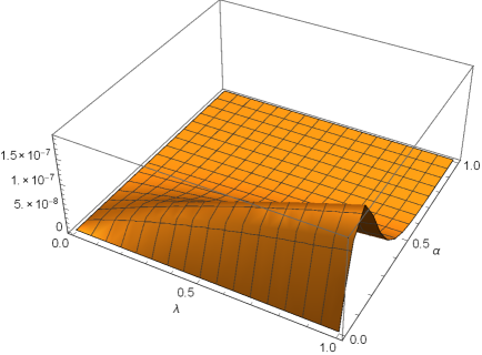
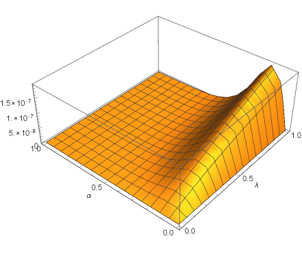
Figure 1. Spectral distribution function $\rho(t)$, Eq.(3.9).

Furthermore, fixing one or the other of the remaining parameter, we obtain the graphics of distribution function $K$ in ${\rm I\!R}^{2}$, as can be seen in Figure 2. In all these graphics we considered a fixed value for $r$ in order to analyse the function’s behavior when we vary the values of its parameters.

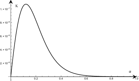
(a) $\lambda=0.5$

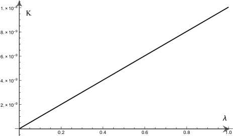
(b) $\alpha=0.5$

Figure 2. Spectral distribution function $\rho(t)$, Eq.(3.9), with a fix parameter.

We use a theorem to demonstrate what we observe in the graphics.

Theorem 3.1.

If $f(t)$ is a locally integrable function in ${\rm I\!R}^{+}$ and CM in $(0,\,\infty)$, then its LT, given by $\mathscr{L}[f(t)](s)=F(s)$, has the following properties:

i) F(s) has an analytic extension in the region ${\rm IC}\setminus{\rm I\!R}^{-}$;
ii) $F(x)=F^{*}(x)$ for $x\in(0,\infty)$;
iii) $\underset{x\rightarrow\infty}{\lim}F(x)=0$;
iv) $\mbox{Im}\{F(s)\}<0$ for $\mbox{Im}\{s\}>0$;
v) $\mbox{Im}\{sF(s)\}\geq 0$ for $\mbox{Im}\{s\}>0$ and $F(x)\geq 0$ for $x\in(0,\infty)$.

Reciprocally, every function $F(s)$ satisfying properties (i)-(iii), together with (iv) or (v), is the LT of a function $f(t)$ locally integrable in ${\rm I\!R}^{+}$ and CM in $(0,\,\infty)$.

Indeed, we have from Eq.(3.4) that the LT of our function, $\tilde{\rho}(s)=\mathscr{L}[E_{\alpha,1}^{\lambda}(-t^{\alpha})](s)$ is given by:

(3.10) $$\tilde{\rho}(s)=\frac{s^{\alpha\lambda-1}}{(s^{\alpha}+1)^{\lambda}}.$$

Hence, conditions (i)-(iii) are evidently satisfied.

Thus, as

(3.11) $$s\tilde{\rho}(s)=\frac{s^{\alpha\lambda}}{(s^{\alpha}+1)^{\lambda}}=\frac{1}{(1+s^{-\alpha})^{\lambda}},$$

we have to show that condition (v) is also satisfied, that is, that for Im$\{s\}>0$ one has $\mbox{Im}\{sF(s)\}\geq 0$.

Let us then write $s=re^{i\phi}$, with $0<\phi\leq\pi$; we get

(3.12) $$s\tilde{\rho}(s)=\frac{1}{(1+(re^{i\phi})^{-\alpha})^{\lambda}}=\frac{(1+r^{-\alpha}e^{i\phi\alpha})^{\lambda}}{|1+r^{-\alpha}e^{-i\phi\alpha}|^{2\lambda}}.$$

Now, putting $\Omega=|1+(re^{i\phi})^{-\alpha}|^{2\lambda}>0$, we have

(3.13) $$\mbox{Im}\{s\tilde{\rho}(s)\}=\frac{1}{\Omega}\mbox{Im}\{(1+r^{-\alpha}e^{i\phi\alpha})^{\lambda}\}.$$

Writing $z:=r^{-\alpha}e^{i\alpha\phi}$ and recalling that $0<\alpha\phi<\pi$, we conclude that $z$ is in the first or second quadrant of the complex plane ($z\in{\rm IC}^{+}$). Hence, adding to $z$ the complex number $u=1$, whose argument is null, we obtain a new complex number which is also in ${\rm IC}^{+}$. Thus, $(1+z)^{\lambda}\in{\rm IC}^{+}$, that is, Im$\{sF(s)\}\geq 0$, as we wanted to demonstrate.

Moreover, as $E_{\alpha,1}^{\lambda}(-t^{\alpha})$ is CM for $0<\alpha\leq 1$ and $0<\lambda\leq 1$, we have, according to Theorem (2.3), that $f(t)=1-E_{\alpha,1}^{\lambda}(-t^{\alpha})$ is a Bernstein function.

4. Kinetic Relaxation Equations

The classical empirical laws associated with Debye (D), Cole-Cole (C-C), Cole-Davidson (C-D) and Havriliak-Negami (H-N) models are, respectively,

(4.1) $$\tilde{\varepsilon}_{D}(s) = \frac{1}{1+\sigma s},$$

(4.2) $$\tilde{\varepsilon}_{CC}(s) = \frac{1}{1+(\sigma s)^{\alpha}},$$

(4.3) $$\tilde{\varepsilon}_{CD}(s) = \frac{1}{(1+\sigma s)^{\beta}},$$

(4.4) $$\tilde{\varepsilon}_{HN}(s) = \frac{1}{(1+(\sigma s)^{\alpha})^{\beta}},$$

where $\alpha,\,\beta,\,\sigma\,\in\,{\rm I\!R}$ and $\alpha,\,\beta\,\in\,\mbox{(}0,1\mbox{]}$.

In the study of relaxation processes in dielectrics it has been discovered, in investigating the approximate linear response function, that the fluctuations in polarization caused by thermal motion are equal to the fluctuations of the macroscopic dipole relaxation function induced by electric fields [38]. Thus, the laws governing the dipole correlation function $\phi(t)$ are directly linked to the macroscopic structural and kinetic properties of a dielectric system, which are represented by function $\varphi(t)$. We may thus equate the relaxation function $\varphi(t)$ and the macroscopic dipole correlation function $\phi(t)$, as follows:

(4.5) $$\varphi(t)\simeq\phi(t)=\frac{\langle\mathcal{M}(t)\mathcal{M}(0)\rangle}{\langle\mathcal{M}(0)\mathcal{M}(0)\rangle},$$

where $\mathcal{M}(t)$ is the macroscopic fluctuating dipole moment. The dipole correlation function defined above is a particular case of the time correlation function studied in the previous section.

From the viewpoint of the modern theory of projection operators developed by Mori [39] and Zwanzig [40], we have the following integrodifferential equation for the time correlation function $\phi(t)$ associated with this memory function $\kappa(t)$, known as memory function equation [41]:

(4.6) $$\frac{d\phi(t)}{dt}=-\int_{0}^{t}\kappa(x)\phi(t-x)dx,$$

Introducing the concept of integral memory function, given by $M(t)=\int_{0}^{t}\kappa(x)dx$ and using the fact that relaxation function $\varphi(t)$ also satisfies Eq.(4.6), we obtain the following relation for function $\varphi(t)$:

(4.7) $$\frac{d\varphi(t)}{dt}=-\frac{d}{dt}\int_{0}^{t}M(t-x)\varphi(x)dx\equiv-\frac{d}{dt}\left[M(t)\ast\varphi(t)\right],$$

where $\ast$ denotes convolution product.

We also know that there exists between relaxation function $\varphi(t)$ and dielectric constant $\tilde{\varepsilon}(s)$ the following relation involving LT:

(4.8) $$\tilde{\varepsilon}(s)=\int_{0}^{\infty}\left(-\frac{d\varphi}{dt}\right)e^{-st}dt=\mathscr{L}\left[-\frac{d\varphi(t)}{dt}\right](s).$$

Thus, from Eq.(4.7), Eq.(4.8) and the empirical laws given by Eqs.(4.1)-(4.4) we obtain the following kinetic relaxation equations:

(4.9) D $$\frac{d\varphi(t)}{dt}+\frac{1}{\sigma}\varphi(t)=0;$$

(4.10) C-C $$\frac{d\varphi(t)}{dt}+\frac{1}{\sigma^{\alpha}}D_{t}^{1-\alpha}\varphi(t)=0;$$

(4.11) C-D $$\frac{d\varphi(t)}{dt}+\frac{1}{\sigma^{\beta}}\frac{d}{dt}\left\{e^{-t/\sigma}\int_{0}^{t}(t-x)^{\beta-1}E_{\beta,\beta}^{1}\left[\left(\frac{t-x}{\sigma}\right)^{\beta}\right]e^{x/\sigma}\varphi(x)dx\right\}=0;$$

(4.12) H-N $$\frac{d}{dt}\left\{\varphi(t)+\sum_{k=0}^{\infty}\int_{0}^{t}\frac{(t-x)^{\alpha\beta(k+1)-1}}{\sigma^{\alpha\beta(k+1)}}E_{\alpha,\alpha\beta(k+1)}^{\beta(k+1)}\left[-\left(\frac{t-x}{\sigma}\right)^{\alpha}\right]\varphi(x)dx\right\}=0.$$

Here, $E_{a,b}^{c}(\cdot)$ are Mittag-Leffler functions and $D_{t}^{\gamma}f(t)$ denotes the fractional differential in the Riemann-Liouville sense, defined by

(4.13) $$D_{t}^{\gamma}f(t)=\frac{1}{\Gamma(1-\gamma)}\frac{d}{dt}\int_{0}^{t}\frac{f(x)}{(t-x)^{\gamma}}dx,\,\,\,\,\,\,\,0<\gamma\leq 1.$$

Let us now consider Eq.(4.12), associated with the H-N model, in the following form:

(4.14) $$\frac{d}{dt}\varphi_{HN}(t)=-\frac{d}{dt}\left\{\left[\sum_{k}\frac{t^{\alpha\beta(k+1)-1}}{\sigma^{\alpha\beta(k+1)}}E_{\alpha,\alpha\beta(k+1)}^{\beta(k+1)}\left[-\left(\frac{t}{\sigma}\right)^{\alpha}\right]\right]*\varphi_{HN}(t)\right\}.$$

Applying LT to Eq.(4.14) we get

(4.15) $$s\tilde{\varphi}_{HN}(s)-1=-s\sum_{k}\frac{1}{(1+(s\sigma)^{\alpha})^{\beta(k+1)}}\cdot\tilde{\varphi}_{HN}(s),$$

where we considered $\varphi_{HN}(0)=1$.

This can be rewritten as

(4.16) $$s\tilde{\varphi}_{HN}(s)-1=-s\frac{\tilde{\varphi}_{HN}(s)}{(1+(s\sigma)^{\alpha})^{\beta}}\sum_{k}\frac{1}{(1+(s\sigma)^{\alpha})^{\beta k}}.$$

Then, calculating the sum on the right-hand side, it follows that

(4.17) $$s\tilde{\varphi}_{HN}(s)-1=-s\frac{\tilde{\varphi}_{HN}(s)}{(1+(s\sigma)^{\alpha})^{\beta}}\frac{1}{1-(1+(s\sigma)^{\alpha})^{-\beta}}.$$

Isolating $\tilde{\varphi}_{HN}(s)$ we get

(4.18) $$\tilde{\varphi}_{HN}(s)=\frac{1}{s}-\frac{1}{\sigma^{-\alpha\beta}}\frac{s^{-1}}{(s^{\alpha}+\sigma^{-\alpha})^{\beta}}.$$

Applying the inverse LT we obtain the solution

(4.19) $$\varphi_{HN}(t)=1-\left(\frac{t}{\sigma}\right)^{\alpha\beta}E_{\alpha,\alpha\beta+1}^{\beta}\left[-\left(\frac{t}{\sigma}\right)^{\alpha}\right].$$

Applying the same procedure to Eqs.(4.9)-(4.11) we obtain their respective solutions:

(4.20) D $$\varphi_{D}(t)=e^{-t/\sigma},$$

(4.21) CC $$\varphi_{CC}(t)=E_{\alpha}\left[-\left(\frac{t}{\sigma}\right)^{\alpha}\right],$$

(4.22) CD $$\varphi_{CD}(t)=1-\left(\frac{t}{\sigma}\right)^{\beta}E_{1,\beta+1}^{\beta}\left[-\frac{t}{\sigma}\right].$$

We can easily see that if we consider $\alpha=1$ in the solution given by Eq.(4.19) we recover the solution given by Eq.(4.22). On the other hand, if we take $\beta=1$ in the solution given by Eq.(4.19), we recover Eq.(4.21). Indeed,

(4.23) $$\varphi_{HN}(t)|_{\beta=1}=1-\left(\frac{t}{\sigma}\right)^{\alpha}E_{\alpha,\alpha+1}\left[-\left(\frac{t}{\sigma}\right)^{\alpha}\right]=1+\sum_{k}\frac{\left[-\left(\frac{t}{\sigma}\right)^{\alpha}\right]^{k+1}}{\Gamma(\alpha(k+1)+1)}.$$

Writing $n=k+1$ in the summation in the second member of Eq.(4.23) we finally get

(4.24) $$\varphi_{HN}(t)|_{\beta=1}=\sum_{n}\frac{\left[-\left(\frac{t}{\sigma}\right)^{\alpha}\right]^{n}}{\Gamma(\alpha n+1)}=\varphi_{CC}(t).$$

Thus, if we consider $\alpha=\beta=1$ in Eq.(4.19) we recover the solution given by Eq.(4.20). Graphic representations of the solutions given by Eq.(4.20), Eq.(4.21) and Eq.(4.22) are shown in Figures 3, 4 and 5, respectively.

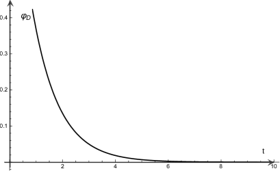
Figure 3. Debye function.

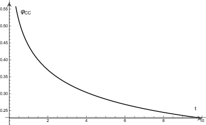
(a) $\alpha=0.4$

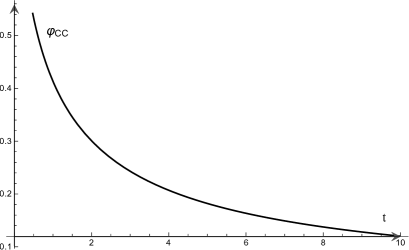
(b) $\alpha=0.6$

Figure 4. Cole-Cole function $\varphi_{CC}(t)=E_{\alpha}(-t^{\alpha})$.

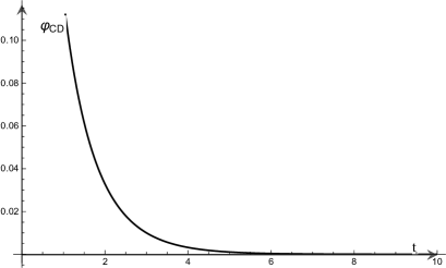
(a) $\beta=0.4$

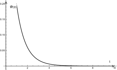
(b) $\beta=0.6$

Figure 5. Cole-Davidson function $\varphi_{CD}(t)=1-t^{\beta}\times E_{1,\beta+1}^{\beta}(-t)$ with $0<\beta<1$.

5. Kinetic Relaxation Functions

In order to make easier the demonstration of the complete monotonicity of these functions, we assume, without loss of generality, that $\sigma=1$. Besides, we must keep in mind that the parameters $\alpha$ and $\beta$ appearing in kinetic relaxation equations belong to the real interval $(0,1]$.

• Beginning with the Debye function, given by $\varphi_{D}(t)=e^{-t}$, we can conclude from the very definition of monotonicity that this function is CM. Indeed,

  (5.1) $$(-1)^{n}D^{n}[\varphi_{D}(t)]=(-1)^{2n}e^{-t}=e^{-t}=\varphi_{D}(t)>0,\,\,\,t\geq 0.$$

  Besides, according to Eq.(2.4) of Theorem (2.4), its spectral distribution function is the Dirac delta function $\delta(r-1)$, that is, it is a positive function.

• Let us now consider C-C function which, as we have seen, is defined by

  (5.2) $$\varphi_{CC}(t)=E_{\alpha}(-t^{\alpha}),\,\,\,\,\mbox{with}\,\,\,\,t\geq 0.$$

  This function is identical to a Mittag-Leffler with a single parameter $\alpha$. On the other hand, this latter function is a particular case of the function given by Eq.(3.3) for $\lambda=1$. In the previous section, we proved its complete monotonicity with the help of Titchmarsh’s formula and Theorem (3.1). We can thus conclude that function $\varphi_{CC}(t)$ is CM for $0<\alpha\leq 1$.
  

• Consider now the C-D function written in the following form:

  (5.3) $$\varphi_{CD}(t)=1-t^{\beta}E_{1,\beta+1}^{\beta}(-t),\,\,\,\,\mbox{with}\,\,\,\,t\geq 0.$$

  This function involves a Mittag-Leffler function with three parameters, one of which is equal to $1$ while the other two are written in terms of $\beta$. We can show that it is CM for $0<\beta<1$.

  Proof.

  Indeed, let $\tilde{\varphi}_{CD}(s)=\mathscr{L}[\varphi_{CD}(t)](s)$, the LT of function $\varphi_{CD}(t)$, given by

  (5.4) $$\tilde{\varphi}_{CD}(s)=\frac{1}{s}\left[1-\frac{1}{(s+1)^{\beta}}\right].$$

  We know that its spectral distribution function has the form

  (5.5) $$K_{\beta}(r)=\frac{1}{\pi}\mbox{Im}\left\{\tilde{\varphi}_{CD}(s)|_{s=re^{-i\pi}}\right\}$$

  This spectral distribution has a branch cut. Hence, $K_{\beta}(r)=0$ when $r<1$ and

  (5.6) $$K_{\beta}(r)=\frac{1}{\pi r}\frac{\hskip 2.0pt\textrm{sin}(\beta\theta)}{(r-1)^{2\beta}},\,\,\,\,\,\mbox{for}\,r>1,$$

  with

  (5.7) $$\theta=\arctan\left(\frac{r\hskip 2.0pt\textrm{sin}\pi}{1+r\hskip 2.0pt\textrm{cos}\pi}\right).$$

  Consider the complex number

  (5.8) $$\rho e^{i\theta}=1+re^{i\pi}.$$

  If we consider $\theta=0$, it follows from the last equation that $\rho=1-r$. This is not a solution because, according to Eq.(5.6), $r>1$ and so $\rho$ would be negative.

  On the other hand, if we choose $\theta=\pi$ in Eq.(5.8) we have $\rho=r-1$; as $r>1$, radius $\rho$ will have positive values.

  Hence,

  (5.9) $$K_{\beta}(r)=\frac{1}{\pi r}\frac{\hskip 2.0pt\textrm{sin}(\beta\pi)}{(r-1)^{2\beta}}.$$

  We conclude that in order to have $K_{\beta}(r)\geq 0$, it is necessary and sufficient that $\beta\pi\in{\rm IC}^{+}$, i.e., that $0<\beta\leq 1$.

• Let us now consider the most general relaxation model and its function, H-N, written in the form

  (5.10) $$\varphi_{HN}(t)=1-t^{\alpha\beta}E_{\alpha,\alpha\beta+1}^{\beta}(-t^{\alpha}),\,\,\,\,\mbox{with}\,\,\,\,t\geq 0.$$

  We shall use Bernstein’s theorem to analyse its complete monotonicity. Also, a graphical analysis will provide some important insights.

  We begin calculating, with the help of Eq.(2.7), the spectral distribution function associated with H-N. We find

  (5.11) $$K_{HN}=\frac{\hskip 2.0pt\textrm{sin}\left[\beta\vartheta\right]}{\pi r(1+2r^{\alpha}\hskip 2.0pt\textrm{cos}(\alpha\pi)+r^{2\alpha})^{\beta/2}},$$

  where $\vartheta=\vartheta(r,\alpha)$ is given by

  (5.12) $$\vartheta=\arctan\left(\frac{r^{\alpha}\hskip 2.0pt\textrm{sin}(\alpha\pi)}{1+r^{\alpha}\hskip 2.0pt\textrm{cos}(\alpha\pi)}\right),\,\,\,\,0<\vartheta\leq\pi.$$

  Since $0<\vartheta\leq\pi$ and $0<\beta\leq 1$, it follows that $0<\beta\vartheta\leq\pi$. This implies that $\hskip 2.0pt\textrm{sin}[\beta\vartheta]\geq 0$. Also, remark that the denominator in the expression of $K_{HN}$ is a positive number and will not influence its sign. We thus conclude that the spectral distribution function $K_{HN}$ associated with the H-N model is everywhere positive.

  Figure 6 presents a plot in ${\rm I\!R}^{3}$ of the spectral distribution function in terms of variables $\alpha$ and $\beta$. It shows that this function is always positive for $0<\alpha\leq 1$ and $0<\beta\leq 1$. In Figures 7 and 8 we fixed one parameter in order to plot the distribution’s behavior as a function of the remaining parameter. In all plots the value of $r$ is held constant.

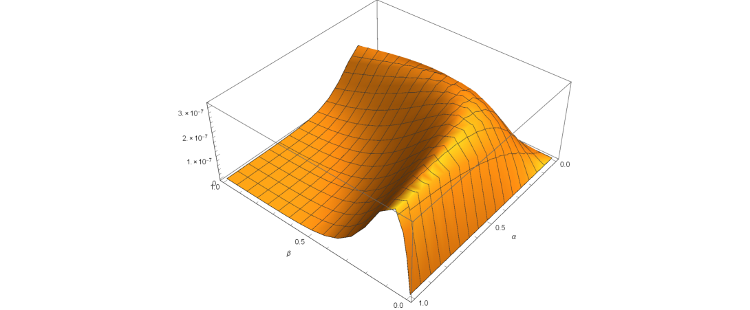
Figure 6. Spectral distribution function H-N according to Eq.(5.11).

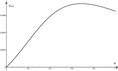
(a) $\beta=0.3$

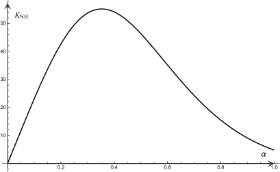
(b) $\beta=0.8$

Figure 7. Spectral distribution function H-N for $0<\alpha\leq 1$, according to Eq.(5.11).

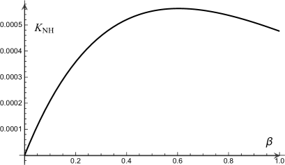
(a) $\alpha=0.3$

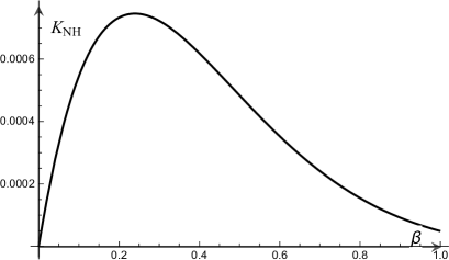
(b) $\alpha=0.8$

Figure 8. Spectral distribution function H-N for $0<\beta\leq 1$, according to Eq.(5.11).

6. Fractional Kinetic Relaxation Functions

Let us now consider the generalization of the relaxation model by means of the fractional differential equation given by

(6.1) $$D_{t}^{\gamma}\varphi(t)=-D_{t}^{\gamma}\left\{M(t)\ast\varphi(t)\right\},\,\,\,\,\mbox{with}\,\gamma\in(0,1],$$

where operator $D_{t}^{\gamma}$ is the fractional derivative in the Riemann-Liouville sense, shown in Eq.(4.13).

In the fractional case, the complex dielectric permissivity (in variable $s$) is given by the following superposition relation [42]:

(6.2) $$\tilde{\varepsilon}(s)=\mathscr{L}\left[-\frac{d^{\gamma}\varphi(t)}{dt}\right](s).$$

Thus, from Eq.(6.1), Eq.(6.2), the normalization condition for relaxation function $\varphi(t)$, given by

(6.3) $$D^{\gamma-1}_{t}\varphi(0)=1,$$

and the classical empirical laws given by Eqs.(4.1)–(4.4), we obtain the memory functions associated with the models by D, C-C, C-D and H-N:

(6.4) D $$M_{D}(t)=\frac{1}{\sigma},$$

(6.5) C-C $$M_{CC}(t)=\frac{t^{\alpha-1}}{\sigma^{\alpha}\Gamma(\alpha)},$$

(6.6) C-D $$M_{CD}(t)=e^{-t/\sigma}\frac{t^{\beta-1}}{\sigma^{\beta}}E_{\beta,\beta}\left[\left(\frac{t}{\sigma}\right)^{\beta}\right],$$

(6.7) H-N $$M_{HN}(t)=\sum_{k=0}^{\infty}\left(\frac{t}{\sigma}\right)^{\alpha\beta(k+1)}t^{-1}E_{\alpha,\alpha\beta(k+1)}^{\beta(k+1)}\left[-\left(\frac{t}{\sigma}\right)^{\alpha}\right],$$

where $\alpha,\,\beta,\,\sigma\,\in\,{\rm I\!R}$ and $\alpha,\,\beta\,\in\,\mbox{(}0,1\mbox{]}$.

From these memory functions we can obtain the fractional kinetic relaxation equations. The solutions of such fractional kinetic relaxation equations are called fractional kinetic relaxation functions. We shall now discuss their monotonicity.

• The solution of the fractional differential equation

  (6.8) $$D^{\gamma}_{t}\varphi_{DF}(t)=-D^{\gamma}_{t}\left\{M_{D}\ast\varphi_{DF}(t)\right\}=-D^{\gamma}_{t}\left\{\frac{1}{\sigma}\ast\varphi_{DF}(t)\right\}$$

  is the fractional Debye function, given by

  (6.9) $$\varphi_{DF}(t)=t^{\gamma-1}E_{1,\gamma}(-t),\,\,\,\,t\geq 0,$$

  with $0<\gamma\leq 1$.

  This function is the product of a power function and a Mittag-Leffler function with two parameters, with the exponent of the power function equal to the second parameter of the Mittag-Leffler function. Figure 9 shows the graphics of this fractional Debye function for two values of $\gamma$. Before analysing this function more thouroughly we shall consider the fractional relaxation function associated with the C-C model.

  

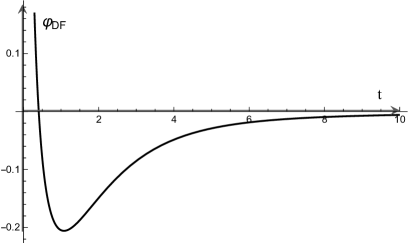
  (a) $\gamma=0.3$

  

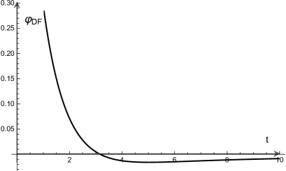
  (b) $\gamma=0.9$

  Figure 9. Function $\varphi_{DF}(t)=t^{\gamma-1}E_{1,\gamma}(-t)$.

• Starting with the C-C fractional kinetic relaxation equation,

  (6.10) $$D^{\gamma}_{t}\varphi_{CCF}(t)=-D^{\gamma}_{t}\left\{M_{CC}\ast\varphi_{CCF}(t)\right\}=-D^{\gamma}_{t}\left\{\frac{t^{\alpha-1}}{\sigma^{\alpha}\Gamma(\alpha)}\ast\varphi_{CCF}(t)\right\},$$

  we obtain its solution, the fractional C-C function,

  (6.11) $$\varphi_{CCF}(t)=t^{\gamma-1}E_{\alpha,\gamma}(-t^{\alpha}),\,\,\,\,\,t\geq 0.$$

  The LT of $\varphi_{CCF}(t)$, denoted by $\tilde{\varphi}_{CCF}(s)=\mathscr{L}[\varphi_{CCF}(t)](s)$, is given by

  (6.12) $$\tilde{\varphi}_{CCF}(s)=\frac{s^{\alpha-\gamma}}{s^{\alpha}+1}$$

  Thus, its distribution function is

  (6.13) $$K_{CCF}=\frac{r^{\alpha-\gamma}}{\pi}\frac{\hskip 2.0pt\textrm{sin}[(\gamma-\alpha)\pi+\theta]}{[r^{2\alpha}+2r^{\alpha}\hskip 2.0pt\textrm{cos}(\alpha\pi)+1]^{1/2}},$$

  where

  (6.14) $$\theta=\arctan\left[\frac{r^{\alpha}\hskip 2.0pt\textrm{sin}(\alpha\pi)}{1+r^{\alpha}\hskip 2.0pt\textrm{cos}(\alpha\pi)}\right].$$

  As $0<\theta<\alpha\pi$, we have $-\alpha\pi<\theta-\alpha\pi<0$ and thus $\gamma\pi-\alpha\pi<\theta+(\gamma-\alpha)\pi<\gamma\pi$. We impose that $\alpha\leq\gamma$ and we know that $0<\alpha,\,\gamma\leq 1$; we thus have $0\leq(\gamma-\alpha)\pi<\theta+(\gamma-\alpha)\pi<\gamma\pi\leq\pi$, i.e. $0<\theta+(\gamma-\alpha)\pi<\pi$. We thus conclude that, if $0<\alpha\leq\gamma\leq 1$, then the sine function in Eq.(6.13) is non-negative and so $K_{CCF}\geq 0$.

  In Figures 10 and 11 we can see the graphic behavior of the spectral distribution function associated with the fractional C-C function. In particular, Figure 11 shows that the spectral distribution function, though very close to zero, becomes positive when $\gamma$ exceeds $\alpha$ (Figure 11(a)); when $\alpha$ exceeds $\gamma$ the function becomes negative (Figure 11(b)).

  In Figures 12 and 13 we can verify, for two different fixed values of $\gamma$, the changes in the function’s behavior according to whether parameter $\alpha$ is smaller or greater than parameter $\gamma$. In both figures, $\alpha<\gamma$ in (a) and (b) and $\alpha>\gamma$ in (c) and (d).

  

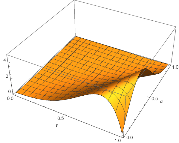
  Figure 10. Spectral distribution associated with fractional C-C function, Eq.(6.13).

  

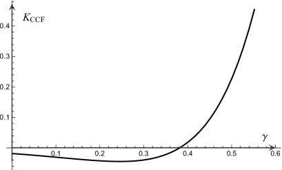
  (a) $\alpha=0.4$

  

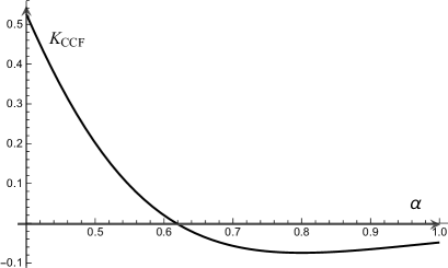
  (b) $\gamma=0.6$

  Figure 11. Spectral distribution associated with fractional C-C function, Eq.(6.13).

  If we choose $\alpha=1$ in the fractional C-C function given by Eq.(6.11), we recover the fractional Debye function given by Eq.(6.9). We can conclude that the fractional Debye function will be CM only if $\gamma=1$, that is, in the integer case.

  

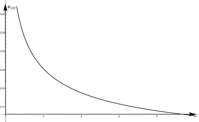
  (a) $\alpha=0.2$

  

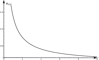
  (b) $\alpha=0.3$

  

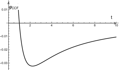
  (c) $\alpha=0.7$

  

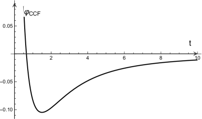
  (d) $\alpha=0.9$

  Figure 12. Function $\varphi_{CCF}(t)=t^{\gamma-1}E_{\alpha,\gamma}(-t^{\alpha})$, for $\gamma=0.4$.

  

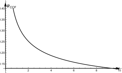
  (a) $\alpha=0.2$

  

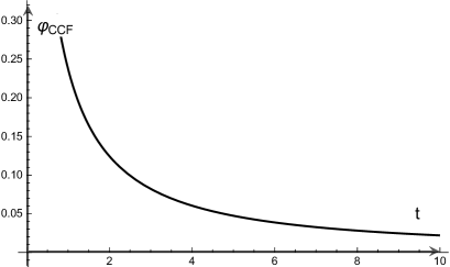
  (b) $\alpha=0.6$

  

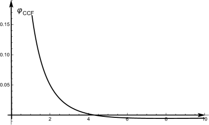
  (c) $\alpha=0.8$

  

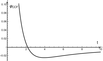
  (d) $\alpha=0.9$

  Figure 13. Function $\varphi_{CCF}(t)=t^{\gamma-1}E_{\alpha,\gamma}(-t^{\alpha})$, for $\gamma=0.7$.

• Now, starting with the equation that generalizes the C-D model, that is,

  (6.15) $$D^{\gamma}_{t}\varphi_{CDF}(t)=-D^{\gamma}_{t}\left\{M_{CD}\ast\varphi_{CDF}(t)\right\}=-D^{\gamma}_{t}\left\{\left[e^{-\frac{t}{\sigma}}\sigma^{-\beta}t^{\beta-1}E_{\beta,\beta}\left[-\left(\frac{t}{\sigma}\right)^{\beta}\right]\right]\ast\varphi_{CDF}(t)\right\},$$

  we find that its soluction, which we call fractional C-D function, has the following form:

  (6.16) $$\varphi_{CDF}(t)=\frac{t^{\gamma-1}}{\Gamma(\gamma)}-t^{\beta+\gamma-1}E_{1,\beta+\gamma}^{\beta}(-t),\,\,\,\,\,\mbox{for}\,\,t\geq 0.$$

  As we can see, this function is formed by the difference between a power function and a product of a power function by a Mittag-Leffler function with three parameters.

  This function is not CM for $\gamma<1$ because we would then have $\alpha=1>\gamma$ and as we shall show in the sequence, graphical evidence suggests that when $\alpha$ is greater than $\gamma$, the function is not CM.

  Figure 14 shows the graphics of several particular cases of this function. As we can see, the function assumes negative values very fast.

  

  (a) $\beta=0.4$ and $\gamma=0.2$

  

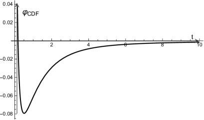
  (b) $\beta=0.2$ and $\gamma=0.4$

  

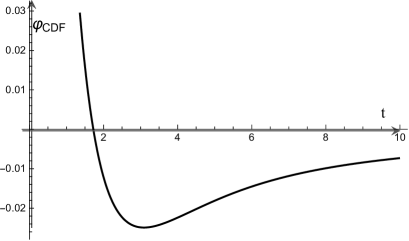
  (c) $\beta=0.6$ and $\gamma=0.8$

  

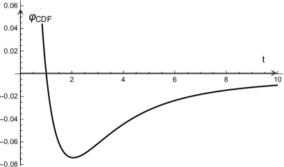
  (d) $\beta=0.8$ and $\gamma=0.6$

  

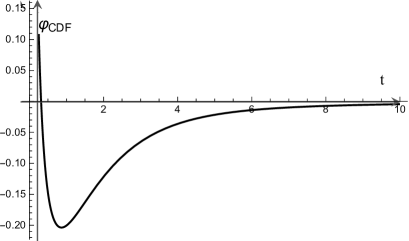
  (e) $\beta=0.8$ and $\gamma=0.3$

  

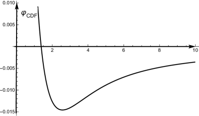
  (f) $\beta=0.3$ and $\gamma=0.8$

  Figure 14. Function $\varphi_{CDF}(t)=\frac{t^{\gamma-1}}{\Gamma(\gamma)}-t^{\beta+\gamma-1}E_{1,\beta+\gamma}^{\beta}(-t)$.

• Finally, let us consider the fractional kinetic relaxation equation

  (6.17) $$D^{\gamma}_{t}\varphi_{HNF}(t)=-D^{\gamma}_{t}\left\{\left[\sum_{k=0}^{\infty}\sigma^{-\alpha k(\beta+1)}t^{\alpha\beta(k+1)-1}E_{\alpha,\alpha\beta(k+1)}^{\beta(k+1)}\left[-\left(\frac{t}{\sigma}\right)^{\alpha}\right]\right]\ast\varphi_{HNF}(t)\right\},$$

  whose solution is the fractional H-N function given by

  (6.18) $$\varphi_{HNF}(t)=\frac{t^{\gamma-1}}{\Gamma(\gamma)}-t^{\alpha\beta+\gamma-1}E_{\alpha,\alpha\beta+\gamma}^{\beta}(-t^{\alpha}),\,\,\,\,\,\mbox{for}\,\,t\geq 0.$$

  Let us now use Titchmarsh’s formula to calculate the spectral distribution of the fractional H-N function. In order to do that, we need to find the LT of the function given by Eq.(6.18). Writing $\tilde{\varphi}_{HNF}(s)=\mathscr{L}[\varphi_{HNF}(t)](s)$ we have

  (6.19) $$\tilde{\varphi}_{HNF}(s)=\frac{1}{s^{\gamma}}-\frac{1}{s^{\gamma}(s^{\alpha}+1)^{\beta}}$$

  Hence, its distribution function is given by

  (6.20) $$K_{HNF}=\frac{1}{\pi r^{\gamma}}\left[\hskip 2.0pt\textrm{sin}(\pi\gamma)-\frac{\hskip 2.0pt\textrm{sin}(\pi\gamma+\beta\theta)}{(r^{2\alpha}+2r^{\alpha}\hskip 2.0pt\textrm{cos}(\alpha\pi)+1)^{\frac{\beta}{2}}}\right],$$

  where

  (6.21) $$\theta=\frac{\pi}{2}-\arctan\left[\frac{1+r^{\alpha}\hskip 2.0pt\textrm{cos}(\alpha\pi)}{r^{\alpha}\hskip 2.0pt\textrm{sin}(\alpha\pi)}\right].$$

  If we consider a very high value for $r$ in Eq.(6.20), the term determining the function’s sign will be $\hskip 2.0pt\textrm{sin}(\pi\gamma)$; it is positive, as $0<\gamma\leq 1$. Thus, in order to investigate the variations of sign of this distribution as a function of its parameters we have drawn the curves shown in Figures 15 and 16 for a small value of $r$. We can see that this distribution function, though very close to zero, becomes negative when parameter $\alpha$ is greater than $\gamma$, the parameter of the fractional derivative, independently of the value of parameter $\beta$. This also explains why the fractional C-D function given by Eq.(6.16) is not CM when $\alpha=1$ and $0<\gamma<1$. We can thus conclude that the fractional C-D function is CM only in the integer case $\gamma=1$. In the case $\alpha=\gamma=1$, as we have seen, this function is CM for $0<\beta\leq 1$.

  

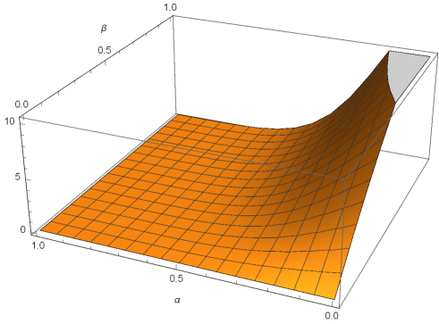
  Figure 15. Distribution function for fractional H-N function for $\gamma=0.7$, according to Eq.(6.20).

  

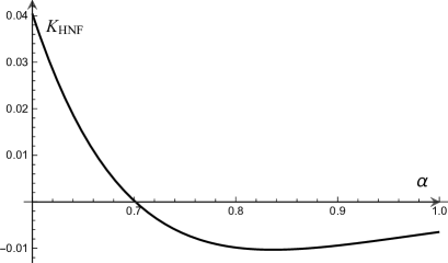
  (a) $\gamma=0.7$, $\beta=0.2$.

  

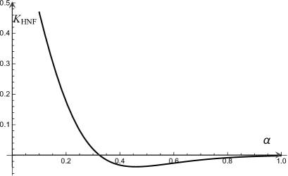
  (b) $\gamma=0.3$, $\beta=0.8$.

  

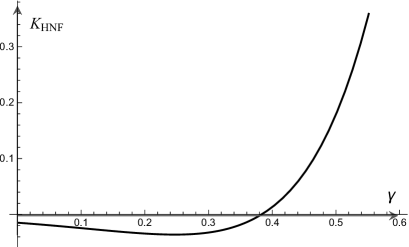
  (c) $\alpha=0.4$, $\beta=0.8$.

  

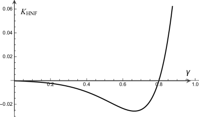
  (d) $\alpha=0.8$, $\beta=0.5$.

  Figure 16. Spectral distribution function for the fractional H-N function, according to Eq.(6.20).

7. Conclusions

The algebraic expressions and the graphic representations of relaxation functions and fractional relaxation functions have shown that their complete monotonicity depends on the parameters appearing in their definitions. We thus analysed the variation of these parameters in order to determine the conditions that should be imposed on them in order to ensure their complete monotonicity.

In the case of Debye’s function, which is independent of those parameters, its complete monotonicity follows directly from its definition. On the other hand, in the case of relaxation functions associated with models C-D, H-N and fractional D and C-C, the study of their complete monotonicity follows from the trigonometric inequality arising from Titchmarsh inversion formula for the spectral distribution function. The function appearing in the C-C model is a particular case of a Mittag-Leffler function with three parameters; its complete monotonicity was demonstrated in the first part of this work, using, among other results, Theorem (3.1). In the case of the relaxation function associated with the fractional H-N model, the associated spectral distribution function has values very close to zero. Nevertheless, the study of its complete monotonicity was based on the graphical analysis of this distribution function. The conclusion about the complete monotonicity of the fractional C-D function is immediate as it is a particular case of fractional H-N function.

References

- [1] S. Bernstein, Sur les fonctions absolument monotones, Acta Math., 52, 1-66, (1929).
- [2] F. Hausdorff, Summationsmethoden und Momentfolgen I, Math. Z., Singapore, 74-109, (1921).
- [3] D. V. Widder, Necessary and sufficient conditions for the representation of a function as a Laplace integral, Trans. Amer. Math. Soc., 40. 851-862, (1931).
- [4] D. V. Widder, The Laplace Transform, Princeton University Press, Princeton, (1946).
- [5] W. Feller, An Introduction to Probability Theory and Its Applications, John Wiley and Sons, New York, (1970).
- [6] C. Li, Y. Chen and J. Kurths, Fractional calculus and its applications, Philos. Trans. A Math. Phys. Eng. Sci., 133, 1990. doi.org/10.1098/rsta.2013.0037, (2013).
- [7] L. Debnath, Recent applications of fractional calculus to science and engineering, Int. J. Math. Math. Sci., 2003:54, 3413-3442. doi:10.1155/S0161171203301486, (2003).
- [8] J. A. Tenreiro Machado, M. F. Silva and R. S. Barbosa, Some applications of fractional calculus in engineering, Math. Probl. Eng., 2010. doi:10.1155/2010/639801, (2010).
- [9] H. Alzer, On some inequalities for the gamma and psi functions, Math. Comp., 66, 373-389, (1997).
- [10] C. Berg and H. L. Pedersen, A completely monotone function related to the gamma function, J. Comp. Appl. Math., 133, 219-230, (2001).
- [11] M. E. H. Ismail and L. Lorch and M. E. Muldoon, Completely monotonic functions associated with the gamma function and its q-analogues, J. Math. Anal. Appl, 116, 1-9, (1986).
- [12] M. Merkle, Completely monotone functions: A Digest, Anal. Num. Theo. Aprox. Theor. Spec. Funct., Springer, New York, 347-364, (2014).
- [13] K. S. Miller and S. G. Samko, A note on the complete monotonicity of the generalized Mittag-Leffler function, Real Anal. Ex., 32, 753-756, 1997.
- [14] K. S. Miller and S. G. Samko, Completely monotonic functions, Integr. Transf. and Spec. Funct., 12:4, 389-402, (2001).
- [15] J. H. An, Fractional calculus, completely monotonic functions, a generalized Mittag-Leffler function and phase-space consistency of separable augmented densities, arXiv preprint arXiv:1201.6113, (2012).
- [16] E. Capelas de Oliveira, F. Mainardi and J. Vaz Jr., Models based on Mittag-Leffler functions for anomalous relaxation in dielectrics, Eur. Phys. J., 193, 161-171, (2014).
- [17] F. Mainardi and R. Garrappa, On complete monotonicity of the Prabhakar function and non-Debye relaxation in dielectrics, J. Comput. Phys., 293, 70-80, (2015).
- [18] T. Simon, Mittag-Leffler functions and complete monotonicity, Int. Transf. and Spec. Func., 26:1, 36-50, (2015).
- [19] J. T. Machado, V. Kiryakova and F. Mainardi, Recent history of fractional calculus, Commun. Nonlinear Sci. Numer. Simul., 16:3, 1140-1153, (2011).
- [20] A. A. Khamzin, R. R. Nigmatullin and I. I. Popov, Justification of the empirical laws of the anomalous dielectric relaxation in the framework of the memory function formalism, Fract. Calc. and Appl. Anal.,17, 247-258, (2014).
- [21] I. Podlubny, Fractional Differential Equations, Academic Press, San Diego, (1999).
- [22] R. Hilfer, Applications of Fractional Calculus in Physics, World Scientific Publishing, Singapore, (2000).
- [23] E. Capelas de Oliveira and R. Figueiredo Camargo, Fractional Calculus (in Portuguese), Livraria da Física, São Paulo, (2015).
- [24] E. Capelas de Oliveira and J. A. Tenreiro Machado, A review of definitions for fractional derivatives and integral, Math. Probl. Eng., 2014, (2014), Article ID 238459, 6 pages.
- [25] F. Mainardi and R. Gorenflo, Time-fractional derivatives in relaxation processes: a tutorial survey, Fract. Calc. and Appl. Anal., 10:3, 269-308, (2007).
- [26] Uchaikin, V.V., Relaxation processes and fractional differential equations, Int. J. Theor. Phys., 42: 121, (2003).
- [27] V.V. Novikov, K. W. Wojciechowski, O. A. Komkova and T. Thiel, Anomalous relaxation in dielectrics. Equations with fractional derivatives, Mater. Sci-Poland, 23:4, 977-984, (2005).
- [28] R. Garrappa, F. Mainardi and G. Maione, Models of dielectric relaxation based on completely monotone functions, Fract. Calc. and Appl. Anal., 19:5, 1105-1160, (2016), doi:10.1515/fca-2016-0060.
- [29] D. Baleanu, J. A. T. Machado and A. C. J. Luo, Fractional Dynamics and Control, Springer, Incorporated, New York, (2012).
- [30] E. C. F. A. Rosa and E. Capelas de Oliveira, Relaxation equations: fractional models, J. Phys. Math., 6:2, 146. doi:10.4172/2090-0902.1000146, (2015).
- [31] G. Gripenberg, Stig-Olof. Londen and O. J. Staffans, Volterra integral and functional equations, Cambridge University Press, New York, (1990).
- [32] H. Pollard, The completely monotonic character of the Mittag-Leffler function , Bull. Amer. Math. Soc., 54:12, 1115-1116, (1948).
- [33] W. R. Schneider, Completely monotone generalized Mittag-Leffler functions, Expositiones Math., 54:14, 003-016, (1996).
- [34] E. C. Titchmarsh, Introduction to the Theory of Fourier Integrals, Oxford University Press, London, (1948).
- [35] E. Capelas de Oliveira, F. Mainardi and J. Vaz Jr., Fractional models of anomalous relaxation based on the Kilbas and Saigo function, Meccanica, 49, 2049-2060, (2014).
- [36] F. Mainardi, Fractional Calculus and Waves in Linear Viscoelasticity, Imperial College Press, London, (2010).
- [37] T. R. Prabhakar, A singular integral equation with a generalized Mittag-Leffler function in the kernel, Yokohama Math. J., 19, 7-15, (1971).
- [38] G. Williams, Use of the dipole correlation function in dielectric relaxation, J. Chem. Rev., 72, 55-69, (1972).
- [39] H. Mori, A continued-fraction representation of the time-correlation functions, Prog. Theor. Phys., 34, 399-416, (1965).
- [40] R. Zwanzig, Lectures in Theoretical Physics, Interscience, New York, (1961).
- [41] J. P. Boon and S. Yip, Molecular Hydrodynamics, Dover, New York, (1980).
- [42] H. Frohlich, Theory of Dielectrics, Oxford University Press, London, (1958).