1 Introduction
This paper concerns with the field enhancement, in other words the gradient blow-up, which occurs due to presence of closely located two perfectly conducting inclusions. If we denote those inclusions by Ω 1 subscript Ω 1 \Omega_{1} Ω 2 subscript Ω 2 \Omega_{2}
{ Δ u = 0 in ℝ 2 ∖ ( Ω 1 ∪ Ω 2 ) ¯ , u = c j on ∂ Ω j , j = 1 , 2 , ∫ ∂ Ω 1 ∂ ν u d s = 0 , j = 1 , 2 , u ( X ) − h ( X ) = O ( | X | − 1 ) as | X | → ∞ . cases Δ 𝑢 0 in superscript ℝ 2 ¯ subscript Ω 1 subscript Ω 2
otherwise formulae-sequence 𝑢 subscript 𝑐 𝑗 on subscript Ω 𝑗
𝑗 1 2
otherwise formulae-sequence subscript subscript Ω 1 subscript 𝜈 𝑢 𝑑 𝑠 0 𝑗 1 2
otherwise formulae-sequence 𝑢 𝑋 ℎ 𝑋 𝑂 superscript 𝑋 1 → as 𝑋 otherwise \begin{cases}\Delta u=0\quad\mbox{in }\mathbb{R}^{2}\setminus\overline{(\Omega_{1}\cup\Omega_{2})},\\
\displaystyle u={c}_{j}\quad\mbox{on }\partial\Omega_{j},\ \ j=1,2,\\
\displaystyle\int_{\partial\Omega_{1}}\partial_{\nu}uds=0,\quad j=1,2,\\
\displaystyle u(X)-h(X)=O(|X|^{-1})\quad\mbox{as }|X|\rightarrow\infty.\end{cases} (1.1)
Here, h ℎ h ℝ 2 superscript ℝ 2 \mathbb{R}^{2} c 1 subscript 𝑐 1 c_{1} c 2 subscript 𝑐 2 c_{2} h ℎ h ∂ Ω j subscript Ω 𝑗 \partial\Omega_{j} 1.1
The problem (1.1 u 𝑢 u ∂ Ω j subscript Ω 𝑗 \partial\Omega_{j} Ω j subscript Ω 𝑗 \Omega_{j} ∞ \infty ∞ \infty u 𝑢 u 1.1
Let u 𝑢 u 1.1
ϵ := dist ( Ω 1 , Ω 2 ) . assign italic-ϵ dist subscript Ω 1 subscript Ω 2 \epsilon:=\mbox{dist}(\Omega_{1},\Omega_{2}). (1.2)
The problem of estimating | ∇ u | ∇ 𝑢 |\nabla u| ϵ italic-ϵ \epsilon [3 ] in relation to stress analysis of composites, and there has been significant progress on this problem in the last decade or so. It is proved that the optimal blow-up rate of | ∇ u | ∇ 𝑢 |\nabla u| ϵ − 1 / 2 superscript italic-ϵ 1 2 \epsilon^{-1/2} [2 , 17 ] , and ( ϵ | ln ϵ | ) − 1 superscript italic-ϵ italic-ϵ 1 (\epsilon|\ln\epsilon|)^{-1} [5 ] . The singular behavior of ∇ u ∇ 𝑢 \nabla u [1 , 10 , 11 , 12 ] .
It is worth mentioning that the gradient estimate was extended to the case of insulating inclusions [2 , 6 , 18 ] , non-homogeneous case [7 ] , p 𝑝 p [8 ] , and the Lamé system of the linear elasticity [4 , 13 ] .
All the above mentioned work deal with inclusions with smooth boundaries, C 2 , α superscript 𝐶 2 𝛼
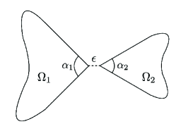
C^{2,\alpha} [16 ] ), and for that it is natural to consider structures consisting of inclusions with corners instead of those with smooth boundaries. One such a structure is the bow-tie structure as depicted in Figure 1
Figure 1: A bow-tie structure
The gradient blow-up due to presence of the bow-tie structure is particularly interesting since two different types of singularities of the gradient are expected: one due to presence of corners and the other due to the interaction between closely located inclusions. Since the fundamental work of Kontratiev [14 ] on the corner singularity (see also [9 , 15 ] ), it is well known that near the vertex of a corner with the aperture angle α 𝛼 \alpha | X − V | − 1 + β superscript 𝑋 𝑉 1 𝛽 |X-V|^{-1+\beta} β = π 2 π − α 𝛽 𝜋 2 𝜋 𝛼 \beta=\frac{\pi}{2\pi-\alpha}
Let V j subscript 𝑉 𝑗 V_{j} Ω j subscript Ω 𝑗 \Omega_{j} V j subscript 𝑉 𝑗 V_{j} α j subscript 𝛼 𝑗 \alpha_{j} j = 1 , 2 𝑗 1 2
j=1,2 1.1 V j subscript 𝑉 𝑗 V_{j}
ϵ − β j | log ϵ | | X − V j | − 1 + β j , superscript italic-ϵ subscript 𝛽 𝑗 italic-ϵ superscript 𝑋 subscript 𝑉 𝑗 1 subscript 𝛽 𝑗 \frac{\epsilon^{-\beta_{j}}}{|\log\epsilon|}|X-V_{j}|^{-1+\beta_{j}}, (1.3)
where
β j := π 2 π − α j , j = 1 , 2 , formulae-sequence assign subscript 𝛽 𝑗 𝜋 2 𝜋 subscript 𝛼 𝑗 𝑗 1 2
\beta_{j}:=\frac{\pi}{2\pi-\alpha_{j}},\quad j=1,2, (1.4)
(see Theorem 5.4 | X − V j | − 1 + β j superscript 𝑋 subscript 𝑉 𝑗 1 subscript 𝛽 𝑗 |X-V_{j}|^{-1+\beta_{j}} ϵ − β j / | log ϵ | superscript italic-ϵ subscript 𝛽 𝑗 italic-ϵ \epsilon^{-\beta_{j}}/|\log\epsilon| 1.3 ϵ − 1 / | log ϵ | superscript italic-ϵ 1 italic-ϵ \epsilon^{-1}/|\log\epsilon| | X − V j | ≤ ϵ 𝑋 subscript 𝑉 𝑗 italic-ϵ |X-V_{j}|\leq\epsilon ϵ − 1 / 2 superscript italic-ϵ 1 2 \epsilon^{-1/2} | ∇ u ( X ) | ∇ 𝑢 𝑋 |\nabla u(X)| X 𝑋 X 5.2
In this paper we assume that the aperture angles α 1 subscript 𝛼 1 \alpha_{1} α 2 subscript 𝛼 2 \alpha_{2} 0 < α j ≤ π 0 subscript 𝛼 𝑗 𝜋 0<\alpha_{j}\leq\pi
C 1 ≤ α 1 + α 2 ≤ 2 π − C 2 subscript 𝐶 1 subscript 𝛼 1 subscript 𝛼 2 2 𝜋 subscript 𝐶 2 C_{1}\leq\alpha_{1}+\alpha_{2}\leq 2\pi-C_{2} (1.5)
for some positive constants C 1 subscript 𝐶 1 C_{1} C 2 subscript 𝐶 2 C_{2} C 1 subscript 𝐶 1 C_{1} C 2 subscript 𝐶 2 C_{2} π 𝜋 \pi
This paper is organized as follows. In section 2 3 4 ∇ u ∇ 𝑢 \nabla u 5
Throughout this paper, the expression A ≲ B less-than-or-similar-to 𝐴 𝐵 A\lesssim B C 𝐶 C ϵ italic-ϵ \epsilon h ℎ h A ≤ C B 𝐴 𝐶 𝐵 A\leq CB A ≃ B similar-to-or-equals 𝐴 𝐵 A\simeq B A ≲ B less-than-or-similar-to 𝐴 𝐵 A\lesssim B B ≲ A less-than-or-similar-to 𝐵 𝐴 B\lesssim A
2 Corner singularities
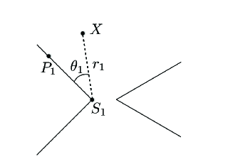
Let Γ 1 subscript Γ 1 \Gamma_{1} S 1 := ( − 1 / 2 , 0 ) assign subscript 𝑆 1 1 2 0 S_{1}:=(-1/2,0) α 1 subscript 𝛼 1 \alpha_{1} S 1 subscript 𝑆 1 S_{1}
Γ 1 = { X = ( x , y ) : | y | < − tan ( α 1 / 2 ) ( x + 1 / 2 ) } , subscript Γ 1 conditional-set 𝑋 𝑥 𝑦 𝑦 subscript 𝛼 1 2 𝑥 1 2 \Gamma_{1}=\{X=(x,y)~{}:~{}|y|<-\tan(\alpha_{1}/2)(x+1/2)\}, (2.1)
and let
Γ 2 = { X = ( x , y ) : | y | < tan ( α 2 / 2 ) ( x − 1 / 2 ) } , subscript Γ 2 conditional-set 𝑋 𝑥 𝑦 𝑦 subscript 𝛼 2 2 𝑥 1 2 \Gamma_{2}=\{X=(x,y)~{}:~{}|y|<\tan(\alpha_{2}/2)(x-1/2)\}, (2.2)
which is the open cone in the right-half space with the vertex at S 2 := ( 1 / 2 , 0 ) assign subscript 𝑆 2 1 2 0 S_{2}:=(1/2,0) α 2 subscript 𝛼 2 \alpha_{2} S 2 subscript 𝑆 2 S_{2} Ω 1 subscript Ω 1 \Omega_{1} Ω 2 subscript Ω 2 \Omega_{2} Γ 1 subscript Γ 1 \Gamma_{1} Γ 2 subscript Γ 2 \Gamma_{2}
L ϵ := 1 2 ( − ϵ + 1 ) and R ϵ := 1 2 ( ϵ − 1 ) . formulae-sequence assign subscript 𝐿 italic-ϵ 1 2 italic-ϵ 1 and
assign subscript 𝑅 italic-ϵ 1 2 italic-ϵ 1 L_{\epsilon}:=\frac{1}{2}(-\epsilon+1)\quad\mbox{and}\quad R_{\epsilon}:=\frac{1}{2}(\epsilon-1). (2.3)
Then, Ω 1 subscript Ω 1 \Omega_{1} Ω 2 subscript Ω 2 \Omega_{2} V 1 := ( − ϵ / 2 , 0 ) assign subscript 𝑉 1 italic-ϵ 2 0 V_{1}:=(-\epsilon/2,0) V 2 := ( ϵ / 2 , 0 ) assign subscript 𝑉 2 italic-ϵ 2 0 V_{2}:=(\epsilon/2,0)
Ω 1 ∩ B δ = ( Γ 1 + L ϵ ) ∩ B δ and Ω 2 ∩ B δ = ( Γ 2 + R ϵ ) ∩ B δ formulae-sequence subscript Ω 1 subscript 𝐵 𝛿 subscript Γ 1 subscript 𝐿 italic-ϵ subscript 𝐵 𝛿 and
subscript Ω 2 subscript 𝐵 𝛿 subscript Γ 2 subscript 𝑅 italic-ϵ subscript 𝐵 𝛿 \Omega_{1}\cap B_{\delta}=(\Gamma_{1}+L_{\epsilon})\cap B_{\delta}\quad\mbox{and}\quad\Omega_{2}\cap B_{\delta}=(\Gamma_{2}+R_{\epsilon})\cap B_{\delta} (2.4)
for some δ > 0 𝛿 0 \delta>0 B δ ( P ) subscript 𝐵 𝛿 𝑃 B_{\delta}(P) δ 𝛿 \delta P 𝑃 P P = O 𝑃 𝑂 P=O B δ subscript 𝐵 𝛿 B_{\delta} Γ 1 subscript Γ 1 \Gamma_{1} Γ 2 subscript Γ 2 \Gamma_{2} ϵ italic-ϵ \epsilon Ω 1 subscript Ω 1 \Omega_{1} Ω 2 subscript Ω 2 \Omega_{2} O 𝑂 O
ϵ ( Γ 1 ∪ Γ 2 ) ∩ B δ = ( Ω 1 ∪ Ω 2 ) ∩ B δ . italic-ϵ subscript Γ 1 subscript Γ 2 subscript 𝐵 𝛿 subscript Ω 1 subscript Ω 2 subscript 𝐵 𝛿 \epsilon(\Gamma_{1}\cup\Gamma_{2})\cap B_{\delta}=(\Omega_{1}\cup\Omega_{2})\cap B_{\delta}.
Figure 2: Polar coordinates with respect to vertices
Choose and fix a point P j subscript 𝑃 𝑗 P_{j} ∂ Γ j ∩ { ( x , y ) : y > 0 } subscript Γ 𝑗 conditional-set 𝑥 𝑦 𝑦 0 \partial\Gamma_{j}\cap\{(x,y):y>0\} j = 1 , 2 𝑗 1 2
j=1,2 θ j ( X ) subscript 𝜃 𝑗 𝑋 \theta_{j}(X) r j ( X ) subscript 𝑟 𝑗 𝑋 r_{j}(X) X ∈ ℝ 2 ∖ Γ j ¯ 𝑋 superscript ℝ 2 ¯ subscript Γ 𝑗 X\in\mathbb{R}^{2}\setminus\overline{\Gamma_{j}} j = 1 , 2 𝑗 1 2
j=1,2
θ j ( X ) = the angle between S j P j → and S j X → , θ j ( X ) = the angle between S j P j → and S j X → \mbox{$\theta_{j}(X)=$the angle between $\overrightarrow{S_{j}P_{j}}$ and $\overrightarrow{S_{j}X}$}, (2.5)
and
r j ( X ) = | X − S j | . subscript 𝑟 𝑗 𝑋 𝑋 subscript 𝑆 𝑗 r_{j}(X)=|X-S_{j}|. (2.6)
See Figure 2 β j subscript 𝛽 𝑗 \beta_{j} 1.4 ℬ j ( X ) subscript ℬ 𝑗 𝑋 \mathcal{B}_{j}(X) j = 1 , 2 𝑗 1 2
j=1,2
ℬ j ( X ) subscript ℬ 𝑗 𝑋 \displaystyle\mathcal{B}_{j}(X) = r j ( X ) β j sin ( β j θ j ( X ) ) , X ∈ ℝ 2 ∖ Γ j ¯ . formulae-sequence absent subscript 𝑟 𝑗 superscript 𝑋 subscript 𝛽 𝑗 subscript 𝛽 𝑗 subscript 𝜃 𝑗 𝑋 𝑋 superscript ℝ 2 ¯ subscript Γ 𝑗 \displaystyle=r_{j}(X)^{\beta_{j}}\sin(\beta_{j}\theta_{j}(X)),\quad X\in\mathbb{R}^{2}\setminus\overline{\Gamma_{j}}\,. (2.7)
The function ℬ j subscript ℬ 𝑗 \mathcal{B}_{j} 2 π − α j 2 𝜋 subscript 𝛼 𝑗 2\pi-\alpha_{j} [9 ] ). Note that ∇ ℬ j ∇ subscript ℬ 𝑗 \nabla\mathcal{B}_{j} β j − 1 subscript 𝛽 𝑗 1 \beta_{j}-1 S j subscript 𝑆 𝑗 S_{j}
| ∇ ℬ j ( X ) | = β j | X − S j | β j − 1 , j = 1 , 2 . formulae-sequence ∇ subscript ℬ 𝑗 𝑋 subscript 𝛽 𝑗 superscript 𝑋 subscript 𝑆 𝑗 subscript 𝛽 𝑗 1 𝑗 1 2
|\nabla\mathcal{B}_{j}(X)|=\beta_{j}|X-S_{j}|^{\beta_{j}-1},\quad j=1,2. (2.8)
Since the bow-tie structure has two corners, the function ℬ 1 − b ℬ 2 subscript ℬ 1 𝑏 subscript ℬ 2 \mathcal{B}_{1}-b\mathcal{B}_{2} b 𝑏 b α 1 subscript 𝛼 1 \alpha_{1} α 2 subscript 𝛼 2 \alpha_{2} 5.3
Lemma 2.1
For j = 1 , 2 𝑗 1 2
j=1,2 ν j subscript 𝜈 𝑗 \nu_{j} ∂ Γ j subscript Γ 𝑗 \partial\Gamma_{j} Γ j subscript Γ 𝑗 \Gamma_{j}
(i)
for X ∈ ∂ Γ 1 ∖ { S 1 } 𝑋 subscript Γ 1 subscript 𝑆 1 X\in\partial\Gamma_{1}\setminus\{S_{1}\}
∂ ν 1 ℬ 1 ( X ) = − | ∇ ℬ 1 ( X ) | < 0 and ∂ ν 1 ℬ 2 ( X ) ≥ 0 , formulae-sequence subscript subscript 𝜈 1 subscript ℬ 1 𝑋 ∇ subscript ℬ 1 𝑋 0 and subscript subscript 𝜈 1 subscript ℬ 2 𝑋
0 \partial_{\nu_{1}}\mathcal{B}_{1}(X)=-|\nabla\mathcal{B}_{1}(X)|<0\quad\mbox{and}\quad\partial_{\nu_{1}}\mathcal{B}_{2}\left(X\right)\geq 0, (2.9)
(ii)
for X ∈ ∂ Γ 2 ∖ { S 2 } 𝑋 subscript Γ 2 subscript 𝑆 2 X\in\partial\Gamma_{2}\setminus\{S_{2}\}
∂ ν 2 ℬ 2 ( X ) = − | ∇ ℬ 2 ( X ) | < 0 and ∂ ν 2 ℬ 1 ( X ) ≥ 0 . formulae-sequence subscript subscript 𝜈 2 subscript ℬ 2 𝑋 ∇ subscript ℬ 2 𝑋 0 and subscript subscript 𝜈 2 subscript ℬ 1 𝑋
0 \partial_{\nu_{2}}\mathcal{B}_{2}\left(X\right)=-\left|\nabla\mathcal{B}_{2}\left(X\right)\right|<0\quad\mbox{and}\quad\partial_{\nu_{2}}\mathcal{B}_{1}\left(X\right)\geq 0. (2.10)
Proof . Let us prove (i) only. (ii) can be proved similarly.
Since ℬ 1 = 0 subscript ℬ 1 0 \mathcal{B}_{1}=0 ∂ Γ 1 subscript Γ 1 \partial\Gamma_{1} ∂ ν 1 ℬ 1 ( X ) ν 1 = ∇ ℬ 1 ( X ) subscript subscript 𝜈 1 subscript ℬ 1 𝑋 subscript 𝜈 1 ∇ subscript ℬ 1 𝑋 \partial_{\nu_{1}}\mathcal{B}_{1}(X)\nu_{1}=\nabla\mathcal{B}_{1}(X) X ∈ ∂ Γ 1 ∖ { S 1 } 𝑋 subscript Γ 1 subscript 𝑆 1 X\in\partial\Gamma_{1}\setminus\{S_{1}\} ℬ 1 > 0 subscript ℬ 1 0 \mathcal{B}_{1}>0 ℝ 2 ∖ Γ 1 ¯ superscript ℝ 2 ¯ subscript Γ 1 \mathbb{R}^{2}\setminus\overline{\Gamma_{1}} ∂ ν 1 ℬ 1 ( X ) < 0 subscript subscript 𝜈 1 subscript ℬ 1 𝑋 0 \partial_{\nu_{1}}\mathcal{B}_{1}(X)<0 2.9
To prove the second inequality in (2.9 X = ( x , y ) 𝑋 𝑥 𝑦 X=(x,y) ℝ 2 ∖ Γ 2 superscript ℝ 2 subscript Γ 2 \mathbb{R}^{2}\setminus\Gamma_{2} S 2 subscript 𝑆 2 S_{2} 2.5 2.6
x − 1 2 = r 2 cos ( θ 2 + α 2 2 ) , y = r 2 sin ( θ 2 + α 2 2 ) . formulae-sequence 𝑥 1 2 subscript 𝑟 2 subscript 𝜃 2 subscript 𝛼 2 2 𝑦 subscript 𝑟 2 subscript 𝜃 2 subscript 𝛼 2 2 x-\frac{1}{2}=r_{2}\cos\left(\theta_{2}+\frac{\alpha_{2}}{2}\right),\quad y=r_{2}\sin\left(\theta_{2}+\frac{\alpha_{2}}{2}\right).
So we see that
U − θ − α 2 / 2 ∇ ℬ 2 ( X ) = ( ∂ r 2 ℬ 2 ( X ) , r 2 − 1 ∂ θ 2 ℬ 2 ( X ) ) T ( T for transpose ) , subscript 𝑈 𝜃 subscript 𝛼 2 2 ∇ subscript ℬ 2 𝑋 superscript subscript subscript 𝑟 2 subscript ℬ 2 𝑋 superscript subscript 𝑟 2 1 subscript subscript 𝜃 2 subscript ℬ 2 𝑋 𝑇 𝑇 for transpose
U_{-\theta-\alpha_{2}/2}\nabla\mathcal{B}_{2}(X)=(\partial_{r_{2}}\mathcal{B}_{2}(X),r_{2}^{-1}\partial_{\theta_{2}}\mathcal{B}_{2}(X))^{T}\ \ (T\mbox{ for transpose}),
where U − θ 2 − α 2 / 2 subscript 𝑈 subscript 𝜃 2 subscript 𝛼 2 2 U_{-\theta_{2}-\alpha_{2}/2} − θ 2 − α 2 / 2 subscript 𝜃 2 subscript 𝛼 2 2 -\theta_{2}-\alpha_{2}/2 S 2 subscript 𝑆 2 S_{2}
∇ ℬ 2 ( X ) = β 2 r 2 β 2 − 1 ( − sin ( θ 2 + α 2 2 − β 2 θ 2 ) , cos ( θ 2 + α 2 2 − β 2 θ 2 ) ) T . ∇ subscript ℬ 2 𝑋 subscript 𝛽 2 superscript subscript 𝑟 2 subscript 𝛽 2 1 superscript subscript 𝜃 2 subscript 𝛼 2 2 subscript 𝛽 2 subscript 𝜃 2 subscript 𝜃 2 subscript 𝛼 2 2 subscript 𝛽 2 subscript 𝜃 2 𝑇 \nabla\mathcal{B}_{2}(X)=\beta_{2}r_{2}^{\beta_{2}-1}\left(-\sin\left(\theta_{2}+\frac{\alpha_{2}}{2}-\beta_{2}\theta_{2}\right),\cos\left(\theta_{2}+\frac{\alpha_{2}}{2}-\beta_{2}\theta_{2}\right)\right)^{T}. (2.11)
One can also see that
ν 1 = − ( sin ( α 1 2 ) , cos ( α 1 2 ) ) T . subscript 𝜈 1 superscript subscript 𝛼 1 2 subscript 𝛼 1 2 𝑇 \nu_{1}=-\left(\sin\left(\frac{\alpha_{1}}{2}\right),\cos\left(\frac{\alpha_{1}}{2}\right)\right)^{T}.
It then follows that
ν 1 ⋅ ∇ ℬ 2 ( X ) = − cos ( ( 1 − β 2 ) θ 2 + α 1 + α 2 2 ) . ⋅ subscript 𝜈 1 ∇ subscript ℬ 2 𝑋 1 subscript 𝛽 2 subscript 𝜃 2 subscript 𝛼 1 subscript 𝛼 2 2 \nu_{1}\cdot\nabla\mathcal{B}_{2}(X)=-\cos\left((1-\beta_{2})\theta_{2}+\frac{\alpha_{1}+\alpha_{2}}{2}\right). (2.12)
If X = ( x , y ) ∈ ∂ Γ 1 𝑋 𝑥 𝑦 subscript Γ 1 X=(x,y)\in\partial\Gamma_{1} y ≥ 0 𝑦 0 y\geq 0
π − α 1 + α 2 2 < θ 2 ( X ) ≤ π − α 2 2 , 𝜋 subscript 𝛼 1 subscript 𝛼 2 2 subscript 𝜃 2 𝑋 𝜋 subscript 𝛼 2 2 \pi-\frac{\alpha_{1}+\alpha_{2}}{2}<\theta_{2}(X)\leq\pi-\frac{\alpha_{2}}{2},
and hence
( 1 − β 2 ) ( π − α 1 + α 2 2 ) + α 1 + α 2 2 1 subscript 𝛽 2 𝜋 subscript 𝛼 1 subscript 𝛼 2 2 subscript 𝛼 1 subscript 𝛼 2 2 \displaystyle(1-\beta_{2})\left(\pi-\frac{\alpha_{1}+\alpha_{2}}{2}\right)+\frac{\alpha_{1}+\alpha_{2}}{2} < ( 1 − β 2 ) θ 2 + α 1 + α 2 2 absent 1 subscript 𝛽 2 subscript 𝜃 2 subscript 𝛼 1 subscript 𝛼 2 2 \displaystyle<(1-\beta_{2})\theta_{2}+\frac{\alpha_{1}+\alpha_{2}}{2}
≤ ( 1 − β 2 ) ( π − α 2 2 ) + α 1 + α 2 2 . absent 1 subscript 𝛽 2 𝜋 subscript 𝛼 2 2 subscript 𝛼 1 subscript 𝛼 2 2 \displaystyle\leq(1-\beta_{2})\left(\pi-\frac{\alpha_{2}}{2}\right)+\frac{\alpha_{1}+\alpha_{2}}{2}.
Note that the term on the far left-hand side is linear in α 1 subscript 𝛼 1 \alpha_{1} α 1 = 0 subscript 𝛼 1 0 \alpha_{1}=0 π 𝜋 \pi π / 2 𝜋 2 \pi/2 π 𝜋 \pi
π 2 < ( 1 − β 2 ) θ 2 + α 1 + α 2 2 < π . 𝜋 2 1 subscript 𝛽 2 subscript 𝜃 2 subscript 𝛼 1 subscript 𝛼 2 2 𝜋 \frac{\pi}{2}<(1-\beta_{2})\theta_{2}+\frac{\alpha_{1}+\alpha_{2}}{2}<\pi.
Now the second inequality in (2.9 2.12 X = ( x , y ) 𝑋 𝑥 𝑦 X=(x,y) y > 0 𝑦 0 y>0 y < 0 𝑦 0 y<0 □ □ \square
The following proposition shows that there is no cancellation between two gradients ∇ ℬ 1 ∇ subscript ℬ 1 \nabla\mathcal{B}_{1} − ∇ ℬ 2 ∇ subscript ℬ 2 -\nabla\mathcal{B}_{2} ∇ ℬ 1 − b ∇ ℬ 2 ∇ subscript ℬ 1 𝑏 ∇ subscript ℬ 2 \nabla\mathcal{B}_{1}-b\nabla\mathcal{B}_{2}
Proposition 2.2
Suppose that b > 0 𝑏 0 b>0
| ∇ ℬ 1 ( X ) | + | ∇ ℬ 2 ( X ) | ≲ | ∇ ℬ 1 ( X ) − b ∇ ℬ 2 ( X ) | less-than-or-similar-to ∇ subscript ℬ 1 𝑋 ∇ subscript ℬ 2 𝑋 ∇ subscript ℬ 1 𝑋 𝑏 ∇ subscript ℬ 2 𝑋 \left|\nabla\mathcal{B}_{1}(X)\right|+\left|\nabla\mathcal{B}_{2}(X)\right|\lesssim\left|\nabla\mathcal{B}_{1}(X)-b\nabla\mathcal{B}_{2}(X)\right| (2.13)
for X ∈ ℝ 2 ∖ Γ 1 ∪ Γ 2 ¯ 𝑋 superscript ℝ 2 ¯ subscript Γ 1 subscript Γ 2 X\in\mathbb{R}^{2}\setminus\overline{\Gamma_{1}\cup\Gamma_{2}}
Proof . We begin the proof by showing that (2.13 ∂ ( B R ∖ ( Γ 1 ∪ Γ 2 ) ) ∖ { S 1 , S 2 } subscript 𝐵 𝑅 subscript Γ 1 subscript Γ 2 subscript 𝑆 1 subscript 𝑆 2 \partial\left(B_{R}\setminus(\Gamma_{1}\cup\Gamma_{2})\right)\setminus\{S_{1},S_{2}\} R > 0 𝑅 0 R>0 l R ± superscript subscript 𝑙 𝑅 plus-or-minus l_{R}^{\pm}
l R ± := { X : X = ( x , y ) ∈ ∂ B R ∖ ( Γ 1 ∪ Γ 2 ) , ± y > 0 } , assign superscript subscript 𝑙 𝑅 plus-or-minus conditional-set 𝑋 formulae-sequence 𝑋 𝑥 𝑦 subscript 𝐵 𝑅 subscript Γ 1 subscript Γ 2 plus-or-minus 𝑦 0 l_{R}^{\pm}:=\left\{X~{}:~{}X=(x,y)\in\partial B_{R}\setminus(\Gamma_{1}\cup\Gamma_{2}),\ \pm y>0\right\},
respectively, so that we have
∂ ( B R ∖ ( Γ 1 ∪ Γ 2 ) ) ∖ { S 1 , S 2 } subscript 𝐵 𝑅 subscript Γ 1 subscript Γ 2 subscript 𝑆 1 subscript 𝑆 2 \displaystyle\partial\left(B_{R}\setminus(\Gamma_{1}\cup\Gamma_{2})\right)\setminus\left\{S_{1},S_{2}\right\}
= l R + ∪ l R − ∪ ( ( ∂ Γ 1 ∩ B R ) ∖ { S 1 } ) ∪ ( ( ∂ Γ 2 ∩ B R ) ∖ { S 2 } ) . absent superscript subscript 𝑙 𝑅 superscript subscript 𝑙 𝑅 subscript Γ 1 subscript 𝐵 𝑅 subscript 𝑆 1 subscript Γ 2 subscript 𝐵 𝑅 subscript 𝑆 2 \displaystyle=l_{R}^{+}\cup l_{R}^{-}\cup((\partial\Gamma_{1}\cap B_{R})\setminus\{S_{1}\})\cup((\partial\Gamma_{2}\cap B_{R})\setminus\{S_{2}\}).
First, we prove (2.13 l R + superscript subscript 𝑙 𝑅 l_{R}^{+} ( r , θ ) 𝑟 𝜃 (r,\theta) O 𝑂 O X = r e i θ 𝑋 𝑟 superscript 𝑒 𝑖 𝜃 X=re^{i\theta} ℝ 2 superscript ℝ 2 \mathbb{R}^{2}
log ( R e i θ − 1 2 ) = log r 2 + i ( θ 2 + α 2 2 ) 𝑅 superscript 𝑒 𝑖 𝜃 1 2 subscript 𝑟 2 𝑖 subscript 𝜃 2 subscript 𝛼 2 2 \log\left(Re^{i\theta}-\frac{1}{2}\right)=\log r_{2}+i\left(\theta_{2}+\frac{\alpha_{2}}{2}\right) (2.14)
on l R + superscript subscript 𝑙 𝑅 l_{R}^{+} | R e i θ − 1 / 2 | = r 2 𝑅 superscript 𝑒 𝑖 𝜃 1 2 subscript 𝑟 2 |Re^{i\theta}-1/2|=r_{2}
r 2 R = 1 + O ( 1 R ) subscript 𝑟 2 𝑅 1 𝑂 1 𝑅 \frac{r_{2}}{R}=1+O\left(\frac{1}{R}\right) (2.15)
for all sufficiently large R 𝑅 R 2.14 θ 𝜃 \theta
R i e i θ R e i θ − 1 2 = 1 r 2 ∂ r 2 ∂ θ + i ∂ θ 2 ∂ θ , 𝑅 𝑖 superscript 𝑒 𝑖 𝜃 𝑅 superscript 𝑒 𝑖 𝜃 1 2 1 subscript 𝑟 2 subscript 𝑟 2 𝜃 𝑖 subscript 𝜃 2 𝜃 \frac{Rie^{i\theta}}{Re^{i\theta}-\frac{1}{2}}=\frac{1}{r_{2}}\frac{\partial r_{2}}{\partial\theta}+i\frac{\partial\theta_{2}}{\partial\theta},
from which we infer that
| ∂ θ 2 ∂ θ − 1 | + 1 r 2 | ∂ r 2 ∂ θ | ≤ C R on l R + , subscript 𝜃 2 𝜃 1 1 subscript 𝑟 2 subscript 𝑟 2 𝜃 𝐶 𝑅 on superscript subscript 𝑙 𝑅
\left|\frac{\partial\theta_{2}}{\partial\theta}-1\right|+\frac{1}{r_{2}}\left|\frac{\partial r_{2}}{\partial\theta}\right|\leq\frac{C}{R}\quad\mbox{on }l_{R}^{+},
provided that R 𝑅 R C 𝐶 C
∂ ℬ 2 ( X ) ∂ θ subscript ℬ 2 𝑋 𝜃 \displaystyle\frac{\partial\mathcal{B}_{2}(X)}{\partial\theta} = ∂ θ 2 ∂ θ ∂ ℬ 2 ( X ) ∂ θ 2 + ∂ r 2 ∂ θ ∂ ℬ 2 ( X ) ∂ r 2 absent subscript 𝜃 2 𝜃 subscript ℬ 2 𝑋 subscript 𝜃 2 subscript 𝑟 2 𝜃 subscript ℬ 2 𝑋 subscript 𝑟 2 \displaystyle=\frac{\partial\theta_{2}}{\partial\theta}\frac{\partial\mathcal{B}_{2}(X)}{\partial\theta_{2}}+\frac{\partial r_{2}}{\partial\theta}\frac{\partial\mathcal{B}_{2}(X)}{\partial r_{2}}
= ( 1 + O ( 1 R ) ) ∂ ℬ 2 ( X ) ∂ θ 2 + O ( 1 R ) r 2 ∂ ℬ 2 ( X ) ∂ r 2 absent 1 𝑂 1 𝑅 subscript ℬ 2 𝑋 subscript 𝜃 2 𝑂 1 𝑅 subscript 𝑟 2 subscript ℬ 2 𝑋 subscript 𝑟 2 \displaystyle=\left(1+O\left(\frac{1}{R}\right)\right)\frac{\partial\mathcal{B}_{2}(X)}{\partial\theta_{2}}+O\left(\frac{1}{R}\right)r_{2}\frac{\partial\mathcal{B}_{2}(X)}{\partial r_{2}} (2.16)
for all sufficiently large R 𝑅 R
One can see that there is R 0 subscript 𝑅 0 R_{0} 0 ≤ β j θ 2 ( X ) ≤ π / 2 − θ 0 0 subscript 𝛽 𝑗 subscript 𝜃 2 𝑋 𝜋 2 subscript 𝜃 0 0\leq\beta_{j}\theta_{2}(X)\leq\pi/2-\theta_{0} θ 0 > 0 subscript 𝜃 0 0 \theta_{0}>0 X ∈ l R + 𝑋 superscript subscript 𝑙 𝑅 X\in l_{R}^{+} R ≥ R 0 𝑅 subscript 𝑅 0 R\geq R_{0}
sin ( β 2 θ 2 ( X ) ) ≤ C cos ( β 2 θ 2 ( X ) ) , subscript 𝛽 2 subscript 𝜃 2 𝑋 𝐶 subscript 𝛽 2 subscript 𝜃 2 𝑋 \sin(\beta_{2}\theta_{2}(X))\leq C\cos(\beta_{2}\theta_{2}(X)),
and hence
0 < r 2 ∂ ℬ 2 ( X ) ∂ r 2 ≤ C ∂ ℬ 2 ( X ) ∂ θ 2 . 0 subscript 𝑟 2 subscript ℬ 2 𝑋 subscript 𝑟 2 𝐶 subscript ℬ 2 𝑋 subscript 𝜃 2 0<r_{2}\frac{\partial\mathcal{B}_{2}(X)}{\partial r_{2}}\leq C\frac{\partial\mathcal{B}_{2}(X)}{\partial\theta_{2}}. (2.17)
This together with (2.16 R 1 subscript 𝑅 1 R_{1}
∂ ℬ 2 ( X ) ∂ θ ≃ ∂ ℬ 2 ( X ) ∂ θ 2 similar-to-or-equals subscript ℬ 2 𝑋 𝜃 subscript ℬ 2 𝑋 subscript 𝜃 2 \frac{\partial\mathcal{B}_{2}(X)}{\partial\theta}\simeq\frac{\partial\mathcal{B}_{2}(X)}{\partial\theta_{2}} (2.18)
for all X ∈ l R + 𝑋 superscript subscript 𝑙 𝑅 X\in l_{R}^{+} R ≥ R 1 𝑅 subscript 𝑅 1 R\geq R_{1}
| ∇ ℬ 2 ( X ) | ≤ C ( 1 r 2 ∂ ℬ 2 ( X ) ∂ θ 2 + ∂ ℬ 2 ( X ) ∂ r 2 ) ≤ C 1 r 2 ∂ ℬ 2 ( X ) ∂ θ 2 . ∇ subscript ℬ 2 𝑋 𝐶 1 subscript 𝑟 2 subscript ℬ 2 𝑋 subscript 𝜃 2 subscript ℬ 2 𝑋 subscript 𝑟 2 𝐶 1 subscript 𝑟 2 subscript ℬ 2 𝑋 subscript 𝜃 2 |\nabla\mathcal{B}_{2}(X)|\leq C\left(\frac{1}{r_{2}}\frac{\partial\mathcal{B}_{2}(X)}{\partial\theta_{2}}+\frac{\partial\mathcal{B}_{2}(X)}{\partial r_{2}}\right)\leq C\frac{1}{r_{2}}\frac{\partial\mathcal{B}_{2}(X)}{\partial\theta_{2}}. (2.19)
It then follows from (2.15 2.18 2.19
| ∇ ℬ 2 ( X ) | ≤ C 1 R ∂ ℬ 2 ( X ) ∂ θ , X ∈ l R + , formulae-sequence ∇ subscript ℬ 2 𝑋 𝐶 1 𝑅 subscript ℬ 2 𝑋 𝜃 𝑋 superscript subscript 𝑙 𝑅 |\nabla\mathcal{B}_{2}(X)|\leq C\frac{1}{R}\frac{\partial\mathcal{B}_{2}(X)}{\partial\theta},\quad X\in l_{R}^{+}, (2.20)
for all R ≥ R 1 𝑅 subscript 𝑅 1 R\geq R_{1}
In the same way, one can show that there is a positive constant C 𝐶 C R 𝑅 R
1 r 1 ∂ ℬ 1 ( X ) ∂ θ 1 ≤ − C 1 R ∂ ℬ 1 ( X ) ∂ θ 1 subscript 𝑟 1 subscript ℬ 1 𝑋 subscript 𝜃 1 𝐶 1 𝑅 subscript ℬ 1 𝑋 𝜃 \frac{1}{r_{1}}\frac{\partial\mathcal{B}_{1}(X)}{\partial\theta_{1}}\leq-C\frac{1}{R}\frac{\partial\mathcal{B}_{1}(X)}{\partial\theta}
and
| ∇ ℬ 1 ( X ) | ≤ − C 1 R ∂ ℬ 1 ( X ) ∂ θ , X ∈ l R + , formulae-sequence ∇ subscript ℬ 1 𝑋 𝐶 1 𝑅 subscript ℬ 1 𝑋 𝜃 𝑋 superscript subscript 𝑙 𝑅 |\nabla\mathcal{B}_{1}(X)|\leq-C\frac{1}{R}\frac{\partial\mathcal{B}_{1}(X)}{\partial\theta},\quad X\in l_{R}^{+}, (2.21)
provided that R ≥ R 1 𝑅 subscript 𝑅 1 R\geq R_{1}
Combining (2.20 2.21
| ∇ ℬ 1 ( X ) | + | ∇ ℬ 2 ( X ) | ∇ subscript ℬ 1 𝑋 ∇ subscript ℬ 2 𝑋 \displaystyle|\nabla\mathcal{B}_{1}(X)|+|\nabla\mathcal{B}_{2}(X)| ≤ − C ( 1 R ∂ ℬ 1 ( X ) ∂ θ − b 1 R ∂ ℬ 2 ( X ) ∂ θ ) absent 𝐶 1 𝑅 subscript ℬ 1 𝑋 𝜃 𝑏 1 𝑅 subscript ℬ 2 𝑋 𝜃 \displaystyle\leq-C\left(\frac{1}{R}\frac{\partial\mathcal{B}_{1}(X)}{\partial\theta}-b\frac{1}{R}\frac{\partial\mathcal{B}_{2}(X)}{\partial\theta}\right)
≤ C | ∇ ℬ 1 ( X ) − b ∇ ℬ 2 ( X ) | on l R + . absent 𝐶 ∇ subscript ℬ 1 𝑋 𝑏 ∇ subscript ℬ 2 𝑋 on superscript subscript 𝑙 𝑅
\displaystyle\leq C\left|\nabla{\mathcal{B}_{1}(X)}-b\nabla{\mathcal{B}_{2}(X)}\right|\quad\mbox{on }l_{R}^{+}.
In the same way, we obtain an analogous estimate on l R − superscript subscript 𝑙 𝑅 l_{R}^{-} R 2 subscript 𝑅 2 R_{2} C > 0 𝐶 0 C>0 R ≥ R 2 𝑅 subscript 𝑅 2 R\geq R_{2}
| ∇ ℬ 1 ( X ) | + | ∇ ℬ 2 ( X ) | ≤ C | ∇ ℬ 1 ( X ) − b ∇ ℬ 2 ( X ) | for all X ∈ l R + ∪ l R − . formulae-sequence ∇ subscript ℬ 1 𝑋 ∇ subscript ℬ 2 𝑋 𝐶 ∇ subscript ℬ 1 𝑋 𝑏 ∇ subscript ℬ 2 𝑋 for all 𝑋 superscript subscript 𝑙 𝑅 superscript subscript 𝑙 𝑅 |\nabla\mathcal{B}_{1}(X)|+|\nabla\mathcal{B}_{2}(X)|\leq C\left|\nabla{\mathcal{B}_{1}(X)}-b\nabla{\mathcal{B}_{2}(X)}\right|\quad\mbox{for all }X\in l_{R}^{+}\cup l_{R}^{-}. (2.22)
Second, we prove (2.13 ( ( ∂ Γ 1 ∩ B R ) ∖ { S 1 } ) subscript Γ 1 subscript 𝐵 𝑅 subscript 𝑆 1 ((\partial\Gamma_{1}\cap B_{R})\setminus\{S_{1}\}) 2.22
| ∇ ℬ 1 ( X ) | + | ∇ ℬ 2 ( X ) | ≤ C | ∇ ℬ 1 ( X ) − b ∇ ℬ 2 ( X ) | for all X ∈ ( ∂ Γ 1 ∪ ∂ Γ 2 ) ∖ B R 2 . formulae-sequence ∇ subscript ℬ 1 𝑋 ∇ subscript ℬ 2 𝑋 𝐶 ∇ subscript ℬ 1 𝑋 𝑏 ∇ subscript ℬ 2 𝑋 for all 𝑋 subscript Γ 1 subscript Γ 2 subscript 𝐵 subscript 𝑅 2 |\nabla\mathcal{B}_{1}(X)|+|\nabla\mathcal{B}_{2}(X)|\leq C\left|\nabla{\mathcal{B}_{1}(X)}-b\nabla{\mathcal{B}_{2}(X)}\right|\quad\mbox{for all }X\in(\partial\Gamma_{1}\cup\partial\Gamma_{2})\setminus B_{R_{2}}. (2.23)
By the equality (2.8 C 𝐶 C α 1 subscript 𝛼 1 \alpha_{1} α 2 subscript 𝛼 2 \alpha_{2}
| ∇ ℬ 2 ( X ) | ≤ C | ∇ ℬ 1 ( X ) | for all X ∈ ( ∂ Γ 1 ∩ B R 2 ) ∖ { S 1 } , formulae-sequence ∇ subscript ℬ 2 𝑋 𝐶 ∇ subscript ℬ 1 𝑋 for all 𝑋 subscript Γ 1 subscript 𝐵 subscript 𝑅 2 subscript 𝑆 1 |\nabla\mathcal{B}_{2}(X)|\leq C|\nabla\mathcal{B}_{1}(X)|\quad\mbox{for all }X\in(\partial\Gamma_{1}\cap B_{R_{2}})\setminus\{S_{1}\}, (2.24)
and
| ∇ ℬ 1 ( X ) | ≤ C | ∇ ℬ 2 ( X ) | for all X ∈ ( ∂ Γ 2 ∩ B R 2 ) ∖ { S 2 } . formulae-sequence ∇ subscript ℬ 1 𝑋 𝐶 ∇ subscript ℬ 2 𝑋 for all 𝑋 subscript Γ 2 subscript 𝐵 subscript 𝑅 2 subscript 𝑆 2 |\nabla\mathcal{B}_{1}(X)|\leq C|\nabla\mathcal{B}_{2}(X)|\quad\mbox{for all }X\in(\partial\Gamma_{2}\cap B_{R_{2}})\setminus\{S_{2}\}. (2.25)
Suppose X ∈ ( ∂ Γ 1 ∩ B R 2 ) ∖ { S 1 } 𝑋 subscript Γ 1 subscript 𝐵 subscript 𝑅 2 subscript 𝑆 1 X\in(\partial\Gamma_{1}\cap B_{R_{2}})\setminus\{S_{1}\} 2.1 2.24
| ∇ ℬ 1 ( X ) | + | ∇ ℬ 2 ( X ) | ≤ C | ∇ ℬ 1 ( X ) | = − C ∂ ν 1 ℬ 1 ( X ) . ∇ subscript ℬ 1 𝑋 ∇ subscript ℬ 2 𝑋 𝐶 ∇ subscript ℬ 1 𝑋 𝐶 subscript subscript 𝜈 1 subscript ℬ 1 𝑋 |\nabla\mathcal{B}_{1}(X)|+|\nabla\mathcal{B}_{2}(X)|\leq C|\nabla\mathcal{B}_{1}(X)|=-C\partial_{\nu_{1}}\mathcal{B}_{1}(X).
Since b > 0 𝑏 0 b>0 ∂ ν 1 ℬ 2 ( X ) ≥ 0 subscript subscript 𝜈 1 subscript ℬ 2 𝑋 0 \partial_{\nu_{1}}\mathcal{B}_{2}\left(X\right)\geq 0 2.9
| ∇ ℬ 1 ( X ) | + | ∇ ℬ 2 ( X ) | ≤ − C ( ∂ ν 1 ℬ 1 ( X ) − b ∂ ν 1 ℬ 2 ( X ) ) ≤ C | ∇ ℬ 1 ( X ) − b ∇ ℬ 2 ( X ) | . ∇ subscript ℬ 1 𝑋 ∇ subscript ℬ 2 𝑋 𝐶 subscript subscript 𝜈 1 subscript ℬ 1 𝑋 𝑏 subscript subscript 𝜈 1 subscript ℬ 2 𝑋 𝐶 ∇ subscript ℬ 1 𝑋 𝑏 ∇ subscript ℬ 2 𝑋 |\nabla\mathcal{B}_{1}(X)|+|\nabla\mathcal{B}_{2}(X)|\leq-C(\partial_{\nu_{1}}\mathcal{B}_{1}(X)-b\partial_{\nu_{1}}\mathcal{B}_{2}(X))\leq C|\nabla\mathcal{B}_{1}(X)-b\nabla\mathcal{B}_{2}(X)|.
Similarly, one can show that (2.13 X ∈ ( ∂ Γ 2 ∩ B R 2 ) ∖ { S 2 } 𝑋 subscript Γ 2 subscript 𝐵 subscript 𝑅 2 subscript 𝑆 2 X\in(\partial\Gamma_{2}\cap B_{R_{2}})\setminus\{S_{2}\} 2.22 2.23 2.13 ∂ ( B R ∖ ( Γ 1 ∪ Γ 2 ) ) ∖ { S 1 , S 2 } subscript 𝐵 𝑅 subscript Γ 1 subscript Γ 2 subscript 𝑆 1 subscript 𝑆 2 \partial\left(B_{R}\setminus(\Gamma_{1}\cup\Gamma_{2})\right)\setminus\{S_{1},S_{2}\} R ≥ R 2 𝑅 subscript 𝑅 2 R\geq R_{2}
If we identify points in the plane with complex numbers, then ∇ ℬ 1 ∇ subscript ℬ 1 \nabla\mathcal{B}_{1} ∇ ℬ 2 ∇ subscript ℬ 2 \nabla\mathcal{B}_{2} ∇ ℬ 1 − b ∇ ℬ 2 ∇ subscript ℬ 1 𝑏 ∇ subscript ℬ 2 \nabla\mathcal{B}_{1}-b\nabla\mathcal{B}_{2} 2.13 ∂ ( B R ∖ ( Γ 1 ∪ Γ 2 ) ) ∖ { S 1 , S 2 } subscript 𝐵 𝑅 subscript Γ 1 subscript Γ 2 subscript 𝑆 1 subscript 𝑆 2 \partial\left(B_{R}\setminus(\Gamma_{1}\cup\Gamma_{2})\right)\setminus\{S_{1},S_{2}\}
| ∇ ℬ 1 ∇ ℬ 1 ( X ) − b ∇ ℬ 2 ( X ) | ≤ C ∇ subscript ℬ 1 ∇ subscript ℬ 1 𝑋 𝑏 ∇ subscript ℬ 2 𝑋 𝐶 \left|\frac{\nabla\mathcal{B}_{1}}{\nabla{\mathcal{B}_{1}(X)}-b\nabla{\mathcal{B}_{2}(X)}}\right|\leq C
for any X ∈ ∂ ( B R ∖ Γ 1 ∪ Γ 2 ¯ ) 𝑋 subscript 𝐵 𝑅 ¯ subscript Γ 1 subscript Γ 2 X\in\partial\left(B_{R}\setminus\overline{\Gamma_{1}\cup\Gamma_{2}}\right) C 𝐶 C R ≥ R 2 𝑅 subscript 𝑅 2 R\geq R_{2}
| ∇ ℬ 1 ( X ) | ≤ C | ∇ ℬ 1 ( X ) − b ∇ ℬ 2 ( X ) | for all X ∈ B R ∖ Γ 1 ∪ Γ 2 ¯ . formulae-sequence ∇ subscript ℬ 1 𝑋 𝐶 ∇ subscript ℬ 1 𝑋 𝑏 ∇ subscript ℬ 2 𝑋 for all 𝑋 subscript 𝐵 𝑅 ¯ subscript Γ 1 subscript Γ 2 \left|\nabla\mathcal{B}_{1}(X)\right|\leq C\left|{\nabla{\mathcal{B}_{1}(X)}-b\nabla{\mathcal{B}_{2}(X)}}\right|\quad\mbox{for all }X\in B_{R}\setminus\overline{\Gamma_{1}\cup\Gamma_{2}}.
Analogously we can derive the above inequality with ℬ 1 subscript ℬ 1 \mathcal{B}_{1} ℬ 2 subscript ℬ 2 \mathcal{B}_{2} C 𝐶 C R 𝑅 R 2.13 □ □ \square
3 Auxiliary functions on cones and their estimates
In this section we construct some auxiliary functions which are used in an essential way for analysing singular behavior of ∇ u ∇ 𝑢 \nabla u u 𝑢 u 1.1 ℝ 2 ∖ Γ 1 ∪ Γ 2 ¯ superscript ℝ 2 ¯ subscript Γ 1 subscript Γ 2 \mathbb{R}^{2}\setminus\overline{\Gamma_{1}\cup\Gamma_{2}} ϵ italic-ϵ \epsilon
Let, for ease of notation,
Π := ℝ 2 ∖ Γ 1 ∪ Γ 2 ¯ and Π + := { ( x , y ) ∈ Π , y > 0 } . formulae-sequence assign Π superscript ℝ 2 ¯ subscript Γ 1 subscript Γ 2 and
assign superscript Π formulae-sequence 𝑥 𝑦 Π 𝑦 0 \Pi:=\mathbb{R}^{2}\setminus\overline{\Gamma_{1}\cup\Gamma_{2}}\quad\mbox{and}\quad\Pi^{+}:=\{(x,y)\in\Pi,~{}y>0\}. (3.1)
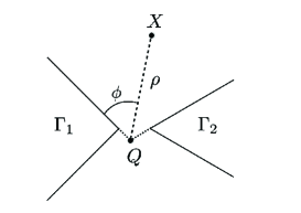
Let P j subscript 𝑃 𝑗 P_{j} ∂ Γ j ∩ { ( x , y ) : y > 0 } subscript Γ 𝑗 conditional-set 𝑥 𝑦 𝑦 0 \partial\Gamma_{j}\cap\{(x,y):y>0\} j = 1 , 2 𝑗 1 2
j=1,2 Q 𝑄 Q P 1 S 1 ¯ ¯ subscript 𝑃 1 subscript 𝑆 1 \overline{P_{1}S_{1}} P 2 S 2 ¯ ¯ subscript 𝑃 2 subscript 𝑆 2 \overline{P_{2}S_{2}} Q 𝑄 Q
Q = ( cot α 1 2 cot α 1 2 + cot α 2 2 − 1 2 , − 1 cot α 1 2 + cot α 2 2 ) . 𝑄 subscript 𝛼 1 2 subscript 𝛼 1 2 subscript 𝛼 2 2 1 2 1 subscript 𝛼 1 2 subscript 𝛼 2 2 Q=\left(\frac{\cot\frac{\alpha_{1}}{2}}{\cot\frac{\alpha_{1}}{2}+\cot\frac{\alpha_{2}}{2}}-\frac{1}{2},-\frac{1}{\cot\frac{\alpha_{1}}{2}+\cot\frac{\alpha_{2}}{2}}\right). (3.2)
We emphasize that Q 𝑄 Q α 1 subscript 𝛼 1 \alpha_{1} α 2 subscript 𝛼 2 \alpha_{2} | Q | → ∞ → 𝑄 |Q|\to\infty α 1 + α 2 → 2 π → subscript 𝛼 1 subscript 𝛼 2 2 𝜋 \alpha_{1}+\alpha_{2}\to 2\pi 1.5 | Q | ≈ 1 𝑄 1 |Q|\approx 1
Figure 3: The polar coordinates ρ 𝜌 \rho ϕ italic-ϕ \phi
Using the point Q 𝑄 Q ϕ ( X ) italic-ϕ 𝑋 \phi(X) X ∈ Π + 𝑋 superscript Π X\in\Pi^{+} Q P 1 → → 𝑄 subscript 𝑃 1 \overrightarrow{QP_{1}} Q X → → 𝑄 𝑋 \overrightarrow{QX}
γ := 2 π 2 π − ( α 1 + α 2 ) . assign 𝛾 2 𝜋 2 𝜋 subscript 𝛼 1 subscript 𝛼 2 \gamma:=\frac{2\pi}{2\pi-(\alpha_{1}+\alpha_{2})}. (3.3)
Then one can easily see that
0 < ϕ < π − 1 2 ( α 1 + α 2 ) = π γ in Π + . formulae-sequence 0 italic-ϕ 𝜋 1 2 subscript 𝛼 1 subscript 𝛼 2 𝜋 𝛾 in superscript Π 0<\phi<\pi-\frac{1}{2}(\alpha_{1}+\alpha_{2})=\frac{\pi}{\gamma}\quad\mbox{in }\Pi^{+}.
We also define ρ = ρ ( X ) 𝜌 𝜌 𝑋 \rho=\rho(X) X 𝑋 X Q 𝑄 Q
ρ ( X ) := | X − Q | . assign 𝜌 𝑋 𝑋 𝑄 \rho(X):=|X-Q|. (3.4)
So, ( ρ , ϕ ) 𝜌 italic-ϕ (\rho,\phi) Q 𝑄 Q Π + superscript Π \Pi^{+} 3
Let w 𝑤 w
{ Δ w = 0 in Π + , w = 0 on ∂ Π + ∖ [ − 1 2 , 1 2 ] × { 0 } , ∂ y w = − ∂ y ϕ on [ − 1 2 , 1 2 ] × { 0 } , ∫ Π + | ∇ w | 2 𝑑 x 𝑑 y < ∞ . cases Δ 𝑤 0 in superscript Π
otherwise 𝑤 0 on superscript Π 1 2 1 2 0
otherwise otherwise subscript 𝑦 𝑤 subscript 𝑦 italic-ϕ on 1 2 1 2 0
otherwise otherwise subscript superscript Π superscript ∇ 𝑤 2 differential-d 𝑥 differential-d 𝑦 otherwise \begin{cases}\Delta w=0\quad\mbox{in }\Pi^{+},\\
w=0\quad\mbox{on }\partial\Pi^{+}\setminus\left[-\frac{1}{2},\frac{1}{2}\right]\times\{0\},\\
\vskip 6.0pt plus 2.0pt minus 2.0pt\cr\partial_{y}w=-\partial_{y}\phi\quad\mbox{on }\left[-\frac{1}{2},\frac{1}{2}\right]\times\{0\},\\
\vskip 6.0pt plus 2.0pt minus 2.0pt\cr\displaystyle\int_{\Pi^{+}}|\nabla w|^{2}dxdy<\infty.\end{cases} (3.5)
We then extend ϕ italic-ϕ \phi w 𝑤 w Π Π \Pi x 𝑥 x
ϕ ( x , y ) = ϕ ( x , − y ) , w ( x , y ) = w ( x , − y ) . formulae-sequence italic-ϕ 𝑥 𝑦 italic-ϕ 𝑥 𝑦 𝑤 𝑥 𝑦 𝑤 𝑥 𝑦 \phi(x,y)=\phi(x,-y),\quad w(x,y)=w(x,-y).
Lemma 3.1
The following holds:
(i)
The function ϕ + w italic-ϕ 𝑤 \phi+w is harmonic in Π Π \Pi , ϕ + w = 0 italic-ϕ 𝑤 0 \phi+w=0 on ∂ Γ 1 subscript Γ 1 \partial\Gamma_{1} , and ϕ + w = π / γ italic-ϕ 𝑤 𝜋 𝛾 \phi+w=\pi/\gamma on ∂ Γ 2 subscript Γ 2 \partial\Gamma_{2} .
(ii)
Let ρ 0 := max { | S 1 − Q | , | S 2 − Q | } assign subscript 𝜌 0 subscript 𝑆 1 𝑄 subscript 𝑆 2 𝑄 \rho_{0}:=\max\{|S_{1}-Q|,|S_{2}-Q|\} . There is a constant C = C ( ρ 0 ) 𝐶 𝐶 subscript 𝜌 0 C=C(\rho_{0}) such that
0 < | ∇ w ( X ) | ≤ C | X ∗ − Q | γ + 1 for all X ∈ Π ∖ B 2 ¯ , formulae-sequence 0 ∇ 𝑤 𝑋 𝐶 superscript superscript 𝑋 𝑄 𝛾 1 for all 𝑋 Π ¯ subscript 𝐵 2 0<|\nabla w(X)|\leq\frac{C}{\left|X^{*}-Q\right|^{{\gamma}+1}}\quad\mbox{for all }X\in\Pi\setminus\overline{B_{2}}, (3.6)
where X ∗ = ( x , | y | ) superscript 𝑋 𝑥 𝑦 X^{*}=(x,|y|) for X = ( x , y ) 𝑋 𝑥 𝑦 X=(x,y) .
(iii)
For each X ∈ Π 𝑋 Π X\in\Pi ,
0 < ( ϕ + w ) ( X ) < π γ . 0 italic-ϕ 𝑤 𝑋 𝜋 𝛾 0<(\phi+w)(X)<\frac{\pi}{\gamma}. (3.7)
Proof . Since ϕ + w italic-ϕ 𝑤 \phi+w Π + superscript Π \Pi^{+} ∂ y ( ϕ + w ) = 0 subscript 𝑦 italic-ϕ 𝑤 0 \partial_{y}(\phi+w)=0 [ − 1 2 , 1 2 ] × { 0 } 1 2 1 2 0 [-\frac{1}{2},\frac{1}{2}]\times\{0\} ϕ + w italic-ϕ 𝑤 \phi+w Π Π \Pi ϕ italic-ϕ \phi w 𝑤 w
To prove (ii) we first observe that the set { X : ρ > ρ 0 , 0 < ϕ < π / γ } conditional-set 𝑋 formulae-sequence 𝜌 subscript 𝜌 0 0 italic-ϕ 𝜋 𝛾 \{X:\rho>\rho_{0},\ 0<\phi<\pi/\gamma\} Π + superscript Π \Pi^{+} 3.5 w 𝑤 w X ∈ Π + 𝑋 superscript Π X\in\Pi^{+} ρ ( X ) > ρ 0 𝜌 𝑋 subscript 𝜌 0 \rho(X)>\rho_{0}
w ( X ) = ∑ n = 1 ∞ a n ρ n γ sin ( n γ ϕ ) . 𝑤 𝑋 superscript subscript 𝑛 1 subscript 𝑎 𝑛 superscript 𝜌 𝑛 𝛾 𝑛 𝛾 italic-ϕ w(X)=\sum_{n=1}^{\infty}\frac{a_{n}}{\rho^{n\gamma}}\sin\left({n\gamma\phi}\right). (3.8)
Since
| ∇ w | 2 = | ∂ ρ w | 2 + ρ − 2 | ∂ ϕ w | 2 , superscript ∇ 𝑤 2 superscript subscript 𝜌 𝑤 2 superscript 𝜌 2 superscript subscript italic-ϕ 𝑤 2 |\nabla w|^{2}=|\partial_{\rho}w|^{2}+\rho^{-2}|\partial_{\phi}w|^{2}, (3.9)
we have
∑ n = 1 ∞ | a n | 2 n γ ρ 0 2 n γ ≲ ∫ ρ 0 ∞ ∫ 0 π / γ | ∇ w | 2 ρ 𝑑 ϕ 𝑑 ρ ≤ ∫ Π + | ∇ w | 2 𝑑 x 𝑑 y < ∞ . less-than-or-similar-to superscript subscript 𝑛 1 superscript subscript 𝑎 𝑛 2 𝑛 𝛾 superscript subscript 𝜌 0 2 𝑛 𝛾 superscript subscript subscript 𝜌 0 superscript subscript 0 𝜋 𝛾 superscript ∇ 𝑤 2 𝜌 differential-d italic-ϕ differential-d 𝜌 subscript superscript Π superscript ∇ 𝑤 2 differential-d 𝑥 differential-d 𝑦 \sum_{n=1}^{\infty}\frac{|a_{n}|^{2}n\gamma}{\rho_{0}^{2n\gamma}}\lesssim\int_{\rho_{0}}^{\infty}\int_{0}^{\pi/\gamma}|\nabla w|^{2}\rho d\phi d\rho\leq\int_{\Pi^{+}}|\nabla w|^{2}dxdy<\infty. (3.10)
If X ∈ Π + ∖ B 2 ¯ 𝑋 superscript Π ¯ subscript 𝐵 2 X\in\Pi^{+}\setminus\overline{B_{2}} ρ ( X ) ≥ ρ 0 + 1 / 2 𝜌 𝑋 subscript 𝜌 0 1 2 \rho(X)\geq\rho_{0}+1/2
| ∇ w ( X ) | ∇ 𝑤 𝑋 \displaystyle\left|\nabla w(X)\right| ≤ C ∑ n = 1 ∞ | a n | n γ ρ n γ + 1 absent 𝐶 superscript subscript 𝑛 1 subscript 𝑎 𝑛 𝑛 𝛾 superscript 𝜌 𝑛 𝛾 1 \displaystyle\leq C\sum_{n=1}^{\infty}|a_{n}|\frac{n\gamma}{\rho^{n\gamma+1}}
≤ C ρ ( ∑ n = 1 ∞ | a n | 2 n γ ρ 0 2 n γ ) 1 2 ( ∑ n = 1 ∞ n γ ( ρ 0 ρ ) 2 n γ ) 1 2 ≤ C ρ γ + 1 , absent 𝐶 𝜌 superscript superscript subscript 𝑛 1 superscript subscript 𝑎 𝑛 2 𝑛 𝛾 superscript subscript 𝜌 0 2 𝑛 𝛾 1 2 superscript superscript subscript 𝑛 1 𝑛 𝛾 superscript subscript 𝜌 0 𝜌 2 𝑛 𝛾 1 2 𝐶 superscript 𝜌 𝛾 1 \displaystyle\leq\frac{C}{\rho}\left(\sum_{n=1}^{\infty}\left|a_{n}\right|^{2}\frac{n\gamma}{\rho_{0}^{2n\gamma}}\right)^{\frac{1}{2}}\left(\sum_{n=1}^{\infty}n\gamma\left(\frac{\rho_{0}}{\rho}\right)^{2n\gamma}\right)^{\frac{1}{2}}\leq\frac{C}{\rho^{\gamma+1}},
that is,
| ∇ w ( X ) | ≤ C | X − Q | γ + 1 . ∇ 𝑤 𝑋 𝐶 superscript 𝑋 𝑄 𝛾 1 \left|\nabla w(X)\right|\leq\frac{C}{\left|X-Q\right|^{{\gamma}+1}}.
Now, (3.6 w 𝑤 w x 𝑥 x
We see from (3.9
∂ ϕ ( ϕ + w ) ( X ) ≥ 1 − | ∂ ϕ w ( X ) | ≥ 1 − ρ ( X ) | ∇ w ( X ) | . subscript italic-ϕ italic-ϕ 𝑤 𝑋 1 subscript italic-ϕ 𝑤 𝑋 1 𝜌 𝑋 ∇ 𝑤 𝑋 \partial_{\phi}\left(\phi+w\right)(X)\geq 1-|\partial_{\phi}w(X)|\geq 1-{\rho(X)}|\nabla w(X)|.
Then (ii) yields
∂ ϕ ( ϕ + w ) ( X ) ≥ 1 − C ρ γ > 1 2 , subscript italic-ϕ italic-ϕ 𝑤 𝑋 1 𝐶 superscript 𝜌 𝛾 1 2 \partial_{\phi}\left(\phi+w\right)(X)\geq 1-\frac{C}{\rho^{\gamma}}>\frac{1}{2},
provided that ρ > ( 2 C ) 1 / γ 𝜌 superscript 2 𝐶 1 𝛾 \rho>(2C)^{1/\gamma} ϕ + w italic-ϕ 𝑤 \phi+w { X : ρ = ρ 1 } conditional-set 𝑋 𝜌 subscript 𝜌 1 \{X:\rho=\rho_{1}\} ρ 1 subscript 𝜌 1 \rho_{1} ρ 1 > ( 2 C ) 1 / γ subscript 𝜌 1 superscript 2 𝐶 1 𝛾 \rho_{1}>(2C)^{1/\gamma} ϕ + w = 0 italic-ϕ 𝑤 0 \phi+w=0 ∂ Γ 1 subscript Γ 1 \partial\Gamma_{1} ϕ + w = π / γ italic-ϕ 𝑤 𝜋 𝛾 \phi+w=\pi/\gamma ∂ Γ 2 subscript Γ 2 \partial\Gamma_{2} 3.7 { X : ρ = ρ 1 } conditional-set 𝑋 𝜌 subscript 𝜌 1 \{X:\rho=\rho_{1}\} ρ 1 subscript 𝜌 1 \rho_{1} ρ 1 > ( 2 C ) 1 / γ subscript 𝜌 1 superscript 2 𝐶 1 𝛾 \rho_{1}>(2C)^{1/\gamma} 3.7 ρ > ( 2 C ) 1 / γ 𝜌 superscript 2 𝐶 1 𝛾 \rho>(2C)^{1/\gamma} ϕ + w italic-ϕ 𝑤 \phi+w x 𝑥 x □ □ \square
Lemma 3.2
There are positive constants a 𝑎 a b 𝑏 b C 𝐶 C
| ∇ ( ϕ + w ) ( X ) − a ( ∇ ℬ 1 − b ∇ ℬ 2 ) ( X ) | ≤ C for all X ∈ Π . formulae-sequence ∇ italic-ϕ 𝑤 𝑋 𝑎 ∇ subscript ℬ 1 𝑏 ∇ subscript ℬ 2 𝑋 𝐶 for all 𝑋 Π |\nabla\left(\phi+w\right)(X)-a\left(\nabla\mathcal{B}_{1}-b\nabla\mathcal{B}_{2}\right)(X)|\leq C\quad\mbox{for all }X\in\Pi. (3.11)
If the aperture angles are the same, namely, α 1 = α 2 subscript 𝛼 1 subscript 𝛼 2 \alpha_{1}=\alpha_{2} b = 1 𝑏 1 b=1
Proof . We first consider the case when X 𝑋 X S 1 subscript 𝑆 1 S_{1} ϕ + w = 0 italic-ϕ 𝑤 0 \phi+w=0 ∂ Γ 1 subscript Γ 1 \partial\Gamma_{1} Γ 1 subscript Γ 1 \Gamma_{1} α 1 = 2 π − π / β 1 subscript 𝛼 1 2 𝜋 𝜋 subscript 𝛽 1 \alpha_{1}=2\pi-\pi/\beta_{1} ϕ + w italic-ϕ 𝑤 \phi+w
( ϕ + w ) ( X ) = a r 1 ( X ) β 1 sin ( β 1 θ 1 ( X ) ) + ∑ n = 2 ∞ a n r 1 ( X ) n β 1 sin ( n β 1 θ 1 ( X ) ) italic-ϕ 𝑤 𝑋 𝑎 subscript 𝑟 1 superscript 𝑋 subscript 𝛽 1 subscript 𝛽 1 subscript 𝜃 1 𝑋 superscript subscript 𝑛 2 subscript 𝑎 𝑛 subscript 𝑟 1 superscript 𝑋 𝑛 subscript 𝛽 1 𝑛 subscript 𝛽 1 subscript 𝜃 1 𝑋 (\phi+w)(X)=ar_{1}(X)^{\beta_{1}}\sin(\beta_{1}\theta_{1}(X))+\sum_{n=2}^{\infty}a_{n}r_{1}(X)^{n\beta_{1}}\sin(n\beta_{1}\theta_{1}(X))
in B 1 ( S 1 ) ∖ Γ 1 ¯ subscript 𝐵 1 subscript 𝑆 1 ¯ subscript Γ 1 B_{1}(S_{1})\setminus{\overline{\Gamma_{1}}} ∑ n = 2 ∞ a n r 1 ( X ) n β 1 sin ( n β 1 θ 1 ( X ) ) superscript subscript 𝑛 2 subscript 𝑎 𝑛 subscript 𝑟 1 superscript 𝑋 𝑛 subscript 𝛽 1 𝑛 subscript 𝛽 1 subscript 𝜃 1 𝑋 \sum_{n=2}^{\infty}a_{n}r_{1}(X)^{n\beta_{1}}\sin(n\beta_{1}\theta_{1}(X)) r 1 < 1 subscript 𝑟 1 1 r_{1}<1 r 1 ≤ r 0 < 1 subscript 𝑟 1 subscript 𝑟 0 1 r_{1}\leq r_{0}<1 r 0 = 0.9 subscript 𝑟 0 0.9 r_{0}=0.9 ℬ 1 = r 1 β 1 sin ( β 1 θ 1 ) subscript ℬ 1 superscript subscript 𝑟 1 subscript 𝛽 1 subscript 𝛽 1 subscript 𝜃 1 \mathcal{B}_{1}=r_{1}^{\beta_{1}}\sin(\beta_{1}\theta_{1})
| ∇ ( ϕ + w ) ( X ) − a ∇ ℬ 1 ( X ) | ≤ C ∇ italic-ϕ 𝑤 𝑋 𝑎 ∇ subscript ℬ 1 𝑋 𝐶 |\nabla(\phi+w)(X)-a\nabla\mathcal{B}_{1}(X)|\leq C (3.12)
for some constant C 𝐶 C X 𝑋 X B 0.9 ( S 1 ) ∖ Γ 1 ¯ subscript 𝐵 0.9 subscript 𝑆 1 ¯ subscript Γ 1 B_{0.9}(S_{1})\setminus\overline{\Gamma_{1}}
Let Γ 1 / 2 subscript Γ 1 2 \Gamma_{1/2} { X : r 1 = 1 / 2 } conditional-set 𝑋 subscript 𝑟 1 1 2 \{X:r_{1}=1/2\} B 1 ( S 1 ) ∖ Γ 1 ¯ subscript 𝐵 1 subscript 𝑆 1 ¯ subscript Γ 1 B_{1}(S_{1})\setminus{\overline{\Gamma_{1}}} a 𝑎 a
a = β 1 2 β 1 + 1 π ∫ Γ 1 / 2 sin ( β 1 θ 1 ) ( ϕ + w ) 𝑑 θ 1 . 𝑎 subscript 𝛽 1 superscript 2 subscript 𝛽 1 1 𝜋 subscript subscript Γ 1 2 subscript 𝛽 1 subscript 𝜃 1 italic-ϕ 𝑤 differential-d subscript 𝜃 1 a=\frac{\beta_{1}2^{\beta_{1}+1}}{\pi}\int_{\Gamma_{1/2}}\sin(\beta_{1}\theta_{1})(\phi+w)d\theta_{1}.
We then infer from (3.7
0 < a < 2 β 1 + 2 γ . 0 𝑎 superscript 2 subscript 𝛽 1 2 𝛾 0<a<\frac{2^{\beta_{1}+2}}{\gamma}. (3.13)
Applying the same argument to ϕ + w − π / γ italic-ϕ 𝑤 𝜋 𝛾 \phi+w-\pi/\gamma B 1 ( S 2 ) ∖ Γ 2 ¯ subscript 𝐵 1 subscript 𝑆 2 ¯ subscript Γ 2 B_{1}(S_{2})\setminus{\overline{\Gamma_{2}}} a ~ ~ 𝑎 \tilde{a}
| ∇ ( ϕ + w ) ( X ) + a ~ ∇ ℬ 2 ( X ) | ≤ C ∇ italic-ϕ 𝑤 𝑋 ~ 𝑎 ∇ subscript ℬ 2 𝑋 𝐶 |\nabla\left(\phi+w\right)(X)+\tilde{a}\nabla\mathcal{B}_{2}(X)|\leq C (3.14)
for all X ∈ B 0.9 ( S 2 ) ∖ Γ 2 ¯ 𝑋 subscript 𝐵 0.9 subscript 𝑆 2 ¯ subscript Γ 2 X\in B_{0.9}(S_{2})\setminus{\overline{\Gamma_{2}}} 0 > ϕ + w − π / γ > − π / γ 0 italic-ϕ 𝑤 𝜋 𝛾 𝜋 𝛾 0>\phi+w-\pi/\gamma>-\pi/\gamma
0 < a ~ < 2 β 2 + 2 γ . 0 ~ 𝑎 superscript 2 subscript 𝛽 2 2 𝛾 0<\tilde{a}<\frac{2^{\beta_{2}+2}}{\gamma}. (3.15)
Let a ~ = a b ~ 𝑎 𝑎 𝑏 \tilde{a}=ab α 1 = α 2 subscript 𝛼 1 subscript 𝛼 2 \alpha_{1}=\alpha_{2} a ~ = a ~ 𝑎 𝑎 \tilde{a}=a b = 1 𝑏 1 b=1
Note that ∇ ℬ 2 ∇ subscript ℬ 2 \nabla\mathcal{B}_{2} B 0.9 ( S 1 ) subscript 𝐵 0.9 subscript 𝑆 1 B_{0.9}(S_{1}) ∇ ℬ 1 ∇ subscript ℬ 1 \nabla\mathcal{B}_{1} B 0.9 ( S 2 ) subscript 𝐵 0.9 subscript 𝑆 2 B_{0.9}(S_{2}) 3.12 3.14
| ∇ ( ϕ + w ) ( X ) − a ( ∇ ℬ 1 − b ∇ ℬ 2 ) ( X ) | ≤ C ∇ italic-ϕ 𝑤 𝑋 𝑎 ∇ subscript ℬ 1 𝑏 ∇ subscript ℬ 2 𝑋 𝐶 |\nabla\left(\phi+w\right)(X)-a\left(\nabla\mathcal{B}_{1}-b\nabla\mathcal{B}_{2}\right)(X)|\leq C (3.16)
for all X ∈ B 0.9 ( S 1 ) ∪ B 0.9 ( S 2 ) ∖ ( Γ 1 ∪ Γ 2 ) ¯ 𝑋 subscript 𝐵 0.9 subscript 𝑆 1 subscript 𝐵 0.9 subscript 𝑆 2 ¯ subscript Γ 1 subscript Γ 2 X\in B_{0.9}(S_{1})\cup B_{0.9}(S_{2})\setminus\overline{\left(\Gamma_{1}\cup\Gamma_{2}\right)}
We now prove (3.11 S 1 subscript 𝑆 1 S_{1} S 2 subscript 𝑆 2 S_{2}
Π 0 := Π ∖ B 0.9 ( S 1 ) ∪ B 0.9 ( S 2 ) . assign subscript Π 0 Π subscript 𝐵 0.9 subscript 𝑆 1 subscript 𝐵 0.9 subscript 𝑆 2 \Pi_{0}:=\Pi\setminus B_{0.9}(S_{1})\cup B_{0.9}(S_{2}).
According to (3.7 ϕ + w italic-ϕ 𝑤 \phi+w ∂ Γ 1 subscript Γ 1 \partial\Gamma_{1} ∂ Γ 2 subscript Γ 2 \partial\Gamma_{2} Π Π \Pi 0 0 π / γ 𝜋 𝛾 \pi/\gamma X 0 ∈ Π 0 subscript 𝑋 0 subscript Π 0 X_{0}\in\Pi_{0} ϕ + w italic-ϕ 𝑤 \phi+w B 1 / 2 ( X 0 ) subscript 𝐵 1 2 subscript 𝑋 0 B_{1/2}(X_{0}) − π / γ 𝜋 𝛾 -\pi/\gamma 2 π / γ 2 𝜋 𝛾 2\pi/\gamma R = 1 / 2 𝑅 1 2 R=1/2
| ∇ ( ϕ + w ) ( X 0 ) | ≤ 2 R ‖ ϕ + w ‖ L ∞ ( B R ( X 0 ) ) ≤ 2 ( 1 2 ) − 1 2 π γ , X 0 ∈ Π 0 . formulae-sequence ∇ italic-ϕ 𝑤 subscript 𝑋 0 2 𝑅 subscript norm italic-ϕ 𝑤 superscript 𝐿 subscript 𝐵 𝑅 subscript 𝑋 0 2 superscript 1 2 1 2 𝜋 𝛾 subscript 𝑋 0 subscript Π 0 \left|\nabla\left(\phi+w\right)(X_{0})\right|\leq\frac{2}{R}\|\phi+w\|_{L^{\infty}(B_{R}(X_{0}))}\leq 2\left(\frac{1}{2}\right)^{-1}\frac{2\pi}{\gamma},\quad X_{0}\in\Pi_{0}. (3.17)
Meanwhile, since Π 0 subscript Π 0 \Pi_{0} 1 / 2 1 2 1/2 S 1 subscript 𝑆 1 S_{1} S 2 subscript 𝑆 2 S_{2}
‖ ∇ ℬ 1 ‖ L ∞ ( Π 0 ) + ‖ ∇ ℬ 2 ‖ L ∞ ( Π 0 ) ≤ C . subscript norm ∇ subscript ℬ 1 superscript 𝐿 subscript Π 0 subscript norm ∇ subscript ℬ 2 superscript 𝐿 subscript Π 0 𝐶 \|\nabla\mathcal{B}_{1}\|_{L^{\infty}(\Pi_{0})}+\|\nabla\mathcal{B}_{2}\|_{L^{\infty}(\Pi_{0})}\leq C.
Therefore, we have for X ∈ Π 0 𝑋 subscript Π 0 X\in\Pi_{0}
| ∇ ( ϕ + w ) ( X ) − a ( ∇ ℬ 1 − b ∇ ℬ 2 ) ( X ) | ∇ italic-ϕ 𝑤 𝑋 𝑎 ∇ subscript ℬ 1 𝑏 ∇ subscript ℬ 2 𝑋 \displaystyle|\nabla\left(\phi+w\right)(X)-a\left(\nabla\mathcal{B}_{1}-b\nabla\mathcal{B}_{2}\right)(X)|
≤ C ( | ∇ ( ϕ + w ) ( X ) | + | ∇ ℬ 1 ( X ) | + | ∇ ℬ 2 ( X ) | ) ≤ C . absent 𝐶 ∇ italic-ϕ 𝑤 𝑋 ∇ subscript ℬ 1 𝑋 ∇ subscript ℬ 2 𝑋 𝐶 \displaystyle\leq C(|\nabla\left(\phi+w\right)(X)|+|\nabla\mathcal{B}_{1}(X)|+|\nabla\mathcal{B}_{2}(X)|)\leq C.
This estimate together with (3.16 3.11 □ □ \square
4 Singular functions and a representation of the solution
In this section we introduce some auxiliary functions on ℝ 2 ∖ ( Ω 1 ∪ Ω 2 ) ¯ superscript ℝ 2 ¯ subscript Ω 1 subscript Ω 2 \mathbb{R}^{2}\setminus\overline{(\Omega_{1}\cup\Omega_{2})} 1.1
Let q 𝑞 q
{ Δ q = 0 in ℝ 2 ∖ ( Ω 1 ∪ Ω 2 ) ¯ , q = d j on ∂ Ω j , j = 1 , 2 , ∫ ∂ Ω 1 ∂ ν q d s = − ∫ ∂ Ω 2 ∂ ν q d s = − 1 , q ( X ) = O ( | X | − 1 ) as | X | → ∞ . cases Δ 𝑞 0 in superscript ℝ 2 ¯ subscript Ω 1 subscript Ω 2
otherwise formulae-sequence 𝑞 subscript 𝑑 𝑗 on subscript Ω 𝑗
𝑗 1 2
otherwise subscript subscript Ω 1 subscript 𝜈 𝑞 𝑑 𝑠 subscript subscript Ω 2 subscript 𝜈 𝑞 𝑑 𝑠 1 otherwise formulae-sequence 𝑞 𝑋 𝑂 superscript 𝑋 1 → as 𝑋 otherwise \begin{cases}\Delta q=0\quad\mbox{in }\mathbb{R}^{2}\setminus\overline{(\Omega_{1}\cup\Omega_{2})},\\
\displaystyle q={d}_{j}\quad\mbox{on }\partial\Omega_{j},\ \ j=1,2,\\
\displaystyle\int_{\partial\Omega_{1}}\partial_{\nu}qds=-\displaystyle\int_{\partial\Omega_{2}}\partial_{\nu}qds=-1,\\
\displaystyle q(X)=O(|X|^{-1})\quad\mbox{as }|X|\rightarrow\infty.\end{cases} (4.1)
Here, d 1 subscript 𝑑 1 d_{1} d 2 subscript 𝑑 2 d_{2} 4.1 ϵ italic-ϵ \epsilon 4.1 [1 ] . It is worth mentioning that
q | ∂ Ω 1 = d 1 < 0 < d 2 = q | ∂ Ω 2 , evaluated-at 𝑞 subscript Ω 1 subscript 𝑑 1 0 subscript bra subscript 𝑑 2 𝑞 subscript Ω 2 q|_{\partial\Omega_{1}}=d_{1}<0<d_{2}=q|_{\partial\Omega_{2}}, (4.2)
which can be seen using Hopf’s lemma.
The singular function of a similar type was first introduced in [17 ] and used to estimate the gradient blow-up when Ω 1 subscript Ω 1 \Omega_{1} Ω 2 subscript Ω 2 \Omega_{2} [1 , 10 ] . If domains have smooth boundaries, then we approximate each of them with the osculating disk. Since the singular function is explicit when Ω j subscript Ω 𝑗 \Omega_{j} q 𝑞 q
However, since the domains under consideration in this paper have corners, such a method do not apply. In this section, we introduce some intermediate auxiliary functions which yield a good approximation of q 𝑞 q
The first intermediate function, η 𝜂 \eta
{ Δ η = 0 in ℝ 2 ∖ ( Ω 1 ∪ Ω 2 ) ¯ , η = 0 on ∂ Ω 1 , η = 1 on ∂ Ω 2 , ∫ ℝ 2 ∖ Ω 1 ∪ Ω 2 ¯ | ∇ η | 2 𝑑 x 𝑑 y < ∞ . cases Δ 𝜂 0 in superscript ℝ 2 ¯ subscript Ω 1 subscript Ω 2
otherwise 𝜂 0 on subscript Ω 1
otherwise 𝜂 1 on subscript Ω 2
otherwise otherwise subscript superscript ℝ 2 ¯ subscript Ω 1 subscript Ω 2 superscript ∇ 𝜂 2 differential-d 𝑥 differential-d 𝑦 otherwise \begin{cases}\Delta\eta=0\quad\mbox{in }\mathbb{R}^{2}\setminus\overline{\left(\Omega_{1}\cup\Omega_{2}\right)},\\
\eta=0\quad\mbox{on }\partial\Omega_{1},\\
\eta=1\quad\mbox{on }\partial\Omega_{2},\\
\vskip 6.0pt plus 2.0pt minus 2.0pt\cr\displaystyle\int_{\mathbb{R}^{2}\setminus\overline{\Omega_{1}\cup\Omega_{2}}}|\nabla\eta|^{2}dxdy<\infty.\end{cases} (4.3)
The connection between q 𝑞 q η 𝜂 \eta
q = ( q | ∂ Ω 2 − q | ∂ Ω 1 ) η + q | ∂ Ω 1 𝑞 evaluated-at 𝑞 subscript Ω 2 evaluated-at 𝑞 subscript Ω 1 𝜂 evaluated-at 𝑞 subscript Ω 1 q=(q|_{\partial\Omega_{2}}-q|_{\partial\Omega_{1}})\eta+q|_{\partial\Omega_{1}} (4.4)
and
∇ q = ( q | ∂ Ω 2 − q | ∂ Ω 1 ) ∇ η . ∇ 𝑞 evaluated-at 𝑞 subscript Ω 2 evaluated-at 𝑞 subscript Ω 1 ∇ 𝜂 \nabla q=(q|_{\partial\Omega_{2}}-q|_{\partial\Omega_{1}})\nabla\eta. (4.5)
We emphasize that (4.4 η 𝜂 \eta 4.3
η ( X ) → a constant , as | X | → ∞ . formulae-sequence → 𝜂 𝑋 a constant → as 𝑋 \eta(X)\to\text{a constant},\quad\text{as }|X|\to\infty. (4.6)
Since Ω j subscript Ω 𝑗 \Omega_{j} x 𝑥 x η 𝜂 \eta ∂ ν η = 0 subscript 𝜈 𝜂 0 \partial_{\nu}\eta=0 V 1 subscript 𝑉 1 V_{1} V 2 subscript 𝑉 2 V_{2} 3.1 η 𝜂 \eta γ π ( ϕ + w ) ( ϵ − 1 X ) 𝛾 𝜋 italic-ϕ 𝑤 superscript italic-ϵ 1 𝑋 \frac{\gamma}{\pi}\left(\phi+w\right)(\epsilon^{-1}X) ϵ − 1 X superscript italic-ϵ 1 𝑋 \epsilon^{-1}X X ∈ B δ ∖ ( Ω 1 ∪ Ω 2 ) 𝑋 subscript 𝐵 𝛿 subscript Ω 1 subscript Ω 2 X\in B_{\delta}\setminus(\Omega_{1}\cup\Omega_{2}) ℝ 2 ∖ ( Γ 1 ∪ Γ 2 ) superscript ℝ 2 subscript Γ 1 subscript Γ 2 \mathbb{R}^{2}\setminus(\Gamma_{1}\cup\Gamma_{2}) L ϵ subscript 𝐿 italic-ϵ L_{\epsilon} R ϵ subscript 𝑅 italic-ϵ R_{\epsilon} 2.3 X − L ϵ 𝑋 subscript 𝐿 italic-ϵ X-L_{\epsilon} B δ ∩ ∂ Ω 1 subscript 𝐵 𝛿 subscript Ω 1 B_{\delta}\cap\partial\Omega_{1} ∂ Γ 1 subscript Γ 1 \partial\Gamma_{1} X − R ϵ 𝑋 subscript 𝑅 italic-ϵ X-R_{\epsilon} B δ ∩ ∂ Ω 2 subscript 𝐵 𝛿 subscript Ω 2 B_{\delta}\cap\partial\Omega_{2} ∂ Γ 2 subscript Γ 2 \partial\Gamma_{2}
Lemma 4.1
Define v ( X ) 𝑣 𝑋 v(X) X ∈ B δ ∖ Ω 1 ∪ Ω 2 ¯ 𝑋 subscript 𝐵 𝛿 ¯ subscript Ω 1 subscript Ω 2 X\in B_{\delta}\setminus\overline{\Omega_{1}\cup\Omega_{2}}
η ( X ) = γ π ( ϕ + w ) ( ϵ − 1 X ) + v ( X ) . 𝜂 𝑋 𝛾 𝜋 italic-ϕ 𝑤 superscript italic-ϵ 1 𝑋 𝑣 𝑋 \eta(X)=\frac{\gamma}{\pi}\left(\phi+w\right)(\epsilon^{-1}X)+v(X). (4.7)
There is δ 1 < δ subscript 𝛿 1 𝛿 \delta_{1}<\delta ϵ italic-ϵ \epsilon
| ∇ v ( X ) | ≲ | ∇ ℬ 1 ( X − L ϵ ) | + | ∇ ℬ 2 ( X − R ϵ ) | , X ∈ B δ 1 ∖ Ω 1 ∪ Ω 2 ¯ . formulae-sequence less-than-or-similar-to ∇ 𝑣 𝑋 ∇ subscript ℬ 1 𝑋 subscript 𝐿 italic-ϵ ∇ subscript ℬ 2 𝑋 subscript 𝑅 italic-ϵ 𝑋 subscript 𝐵 subscript 𝛿 1 ¯ subscript Ω 1 subscript Ω 2 |\nabla v(X)|\lesssim|\nabla\mathcal{B}_{1}(X-L_{\epsilon})|+|\nabla\mathcal{B}_{2}(X-R_{\epsilon})|,\quad X\in B_{\delta_{1}}\setminus\overline{\Omega_{1}\cup\Omega_{2}}. (4.8)
Proof . We first prove that there are constants δ 1 < δ subscript 𝛿 1 𝛿 \delta_{1}<\delta C 1 subscript 𝐶 1 C_{1} C 2 subscript 𝐶 2 C_{2} ϵ italic-ϵ \epsilon
| ∇ v ( X ) | ≤ C 1 | ∇ ℬ 1 ( X − L ϵ ) − ∇ ℬ 2 ( X − R ϵ ) + C 2 ( x + 1 2 , y ) | ∇ 𝑣 𝑋 subscript 𝐶 1 ∇ subscript ℬ 1 𝑋 subscript 𝐿 italic-ϵ ∇ subscript ℬ 2 𝑋 subscript 𝑅 italic-ϵ subscript 𝐶 2 𝑥 1 2 𝑦 |\nabla v(X)|\leq C_{1}\left|\nabla\mathcal{B}_{1}(X-L_{\epsilon})-\nabla\mathcal{B}_{2}(X-R_{\epsilon})+C_{2}\left(x+\frac{1}{2},y\right)\right| (4.9)
for all X ∈ ∂ ( B δ 1 ∖ ( Ω 1 ∪ Ω 2 ) ) 𝑋 subscript 𝐵 subscript 𝛿 1 subscript Ω 1 subscript Ω 2 X\in\partial(B_{\delta_{1}}\setminus(\Omega_{1}\cup\Omega_{2}))
To prove (4.9 ∂ Ω 1 subscript Ω 1 \partial\Omega_{1} ∂ Ω 2 subscript Ω 2 \partial\Omega_{2} O 𝑂 O v 1 + subscript 𝑣 limit-from 1 v_{1+} v 1 − subscript 𝑣 limit-from 1 v_{1-}
{ Δ v 1 + = Δ v 1 − = 0 in B δ ∖ Ω 1 ¯ , v 1 + = v 1 − = 0 on ∂ Ω 1 ∩ B δ , v 1 + = − v 1 − = 4 on ∂ B δ ∖ Ω 1 ¯ , cases Δ subscript 𝑣 limit-from 1 Δ subscript 𝑣 limit-from 1 0 in subscript 𝐵 𝛿 ¯ subscript Ω 1 subscript 𝑣 limit-from 1 subscript 𝑣 limit-from 1 0 on subscript Ω 1 subscript 𝐵 𝛿 subscript 𝑣 limit-from 1 subscript 𝑣 limit-from 1 4 on subscript 𝐵 𝛿 ¯ subscript Ω 1 \begin{cases}\displaystyle\Delta v_{1+}=\Delta v_{1-}=0\quad&\mbox{in }B_{\delta}\setminus\overline{\Omega_{1}},\\
\displaystyle v_{1+}=v_{1-}=0\quad&\mbox{on }\partial\Omega_{1}\cap B_{\delta},\\
\displaystyle v_{1+}=-v_{1-}=4\quad&\mbox{on }\partial B_{\delta}\setminus\overline{\Omega_{1}},\end{cases} (4.10)
and v 2 + subscript 𝑣 limit-from 2 v_{2+} v 2 − subscript 𝑣 limit-from 2 v_{2-}
{ Δ v 2 + = Δ v 2 − = 0 in B δ ∖ Ω 2 ¯ , v 2 + = v 2 − = 0 on ∂ Ω 2 ∩ B δ , v 2 + = − v 2 − = 4 on ∂ B δ ∖ Ω 2 ¯ . cases Δ subscript 𝑣 limit-from 2 Δ subscript 𝑣 limit-from 2 0 in subscript 𝐵 𝛿 ¯ subscript Ω 2 subscript 𝑣 limit-from 2 subscript 𝑣 limit-from 2 0 on subscript Ω 2 subscript 𝐵 𝛿 subscript 𝑣 limit-from 2 subscript 𝑣 limit-from 2 4 on subscript 𝐵 𝛿 ¯ subscript Ω 2 \begin{cases}\displaystyle\Delta v_{2+}=\Delta v_{2-}=0\quad&\mbox{in }B_{\delta}\setminus\overline{\Omega_{2}},\\
\displaystyle v_{2+}=v_{2-}=0\quad&\mbox{on }\partial\Omega_{2}\cap B_{\delta},\\
\displaystyle v_{2+}=-v_{2-}=4\quad&\mbox{on }\partial B_{\delta}\setminus\overline{\Omega_{2}}.\end{cases} (4.11)
Note that v 1 + − v subscript 𝑣 limit-from 1 𝑣 v_{1+}-v v 1 − − v subscript 𝑣 limit-from 1 𝑣 v_{1-}-v ∂ Ω 1 ∩ B δ subscript Ω 1 subscript 𝐵 𝛿 \partial\Omega_{1}\cap B_{\delta}
∂ ν v 1 + < ∂ ν v < ∂ ν v 1 − on ∂ Ω 1 ∩ B δ . formulae-sequence subscript 𝜈 subscript 𝑣 limit-from 1 subscript 𝜈 𝑣 subscript 𝜈 subscript 𝑣 limit-from 1 on subscript Ω 1 subscript 𝐵 𝛿 \partial_{\nu}v_{1+}<\partial_{\nu}v<\partial_{\nu}v_{1-}\quad\mbox{on }\partial\Omega_{1}\cap B_{\delta}. (4.12)
In the same way, we also have
∂ ν v 2 + < ∂ ν v < ∂ ν v 2 − on ∂ Ω 2 ∩ B δ . formulae-sequence subscript 𝜈 subscript 𝑣 limit-from 2 subscript 𝜈 𝑣 subscript 𝜈 subscript 𝑣 limit-from 2 on subscript Ω 2 subscript 𝐵 𝛿 \partial_{\nu}v_{2+}<\partial_{\nu}v<\partial_{\nu}v_{2-}\quad\mbox{on }\partial\Omega_{2}\cap B_{\delta}. (4.13)
Let δ 2 subscript 𝛿 2 \delta_{2} B δ 2 ( V 1 ) ¯ ∖ Ω 1 ¯ ⊂ B δ ∖ Ω 1 ¯ ¯ subscript 𝐵 subscript 𝛿 2 subscript 𝑉 1 ¯ subscript Ω 1 subscript 𝐵 𝛿 ¯ subscript Ω 1 \overline{B_{\delta_{2}}(V_{1})}\setminus\overline{\Omega_{1}}\subset B_{\delta}\setminus\overline{\Omega_{1}} B δ 2 ( V 2 ) ¯ ∖ Ω 2 ¯ ⊂ B δ ∖ Ω 2 ¯ ¯ subscript 𝐵 subscript 𝛿 2 subscript 𝑉 2 ¯ subscript Ω 2 subscript 𝐵 𝛿 ¯ subscript Ω 2 \overline{B_{\delta_{2}}(V_{2})}\setminus\overline{\Omega_{2}}\subset B_{\delta}\setminus\overline{\Omega_{2}} v 1 + = 0 subscript 𝑣 limit-from 1 0 v_{1+}=0 ∂ Ω 1 ∩ B δ subscript Ω 1 subscript 𝐵 𝛿 \partial\Omega_{1}\cap B_{\delta} a 𝑎 a C 3 subscript 𝐶 3 C_{3} ψ 𝜓 \psi v 1 + subscript 𝑣 limit-from 1 v_{1+}
v 1 + ( X ) = a ℬ 1 ( X − L ϵ ) + ψ ( X ) subscript 𝑣 limit-from 1 𝑋 𝑎 subscript ℬ 1 𝑋 subscript 𝐿 italic-ϵ 𝜓 𝑋 v_{1+}(X)=a\mathcal{B}_{1}(X-L_{\epsilon})+\psi(X) (4.14)
and
| ∇ ψ ( X ) | ≤ C 3 for all X ∈ B δ 2 ( V 1 ) ¯ ∖ Ω 1 . formulae-sequence ∇ 𝜓 𝑋 subscript 𝐶 3 for all 𝑋 ¯ subscript 𝐵 subscript 𝛿 2 subscript 𝑉 1 subscript Ω 1 |\nabla\psi(X)|\leq C_{3}\quad\mbox{for all }X\in\overline{B_{\delta_{2}}(V_{1})}\setminus\Omega_{1}. (4.15)
In fact, ψ 𝜓 \psi
ψ ( X ) = ∑ n = 2 ∞ a n r 1 ( X − L ϵ ) n β 1 sin ( n β 1 θ 1 ( X − L ϵ ) ) 𝜓 𝑋 superscript subscript 𝑛 2 subscript 𝑎 𝑛 subscript 𝑟 1 superscript 𝑋 subscript 𝐿 italic-ϵ 𝑛 subscript 𝛽 1 𝑛 subscript 𝛽 1 subscript 𝜃 1 𝑋 subscript 𝐿 italic-ϵ \psi(X)=\sum_{n=2}^{\infty}a_{n}r_{1}(X-L_{\epsilon})^{n\beta_{1}}\sin\big{(}n\beta_{1}\theta_{1}(X-L_{\epsilon}))
for some constants a n subscript 𝑎 𝑛 a_{n} X 𝑋 X | X − L ϵ | < δ 2 + s 𝑋 subscript 𝐿 italic-ϵ subscript 𝛿 2 𝑠 |X-L_{\epsilon}|<\delta_{2}+s s > 0 𝑠 0 s>0 4.15
Note that there is a constant C 4 > 0 subscript 𝐶 4 0 C_{4}>0
| ∇ ℬ 1 ( X − L ϵ ) | ≥ C 4 for all X ∈ B δ 2 ( V 1 ) ¯ ∖ Ω 1 . formulae-sequence ∇ subscript ℬ 1 𝑋 subscript 𝐿 italic-ϵ subscript 𝐶 4 for all 𝑋 ¯ subscript 𝐵 subscript 𝛿 2 subscript 𝑉 1 subscript Ω 1 |\nabla\mathcal{B}_{1}(X-L_{\epsilon})|\geq C_{4}\quad\mbox{for all }X\in\overline{B_{\delta_{2}}(V_{1})}\setminus\Omega_{1}.
So, we infer from (4.14 4.15
| ∇ v 1 + ( X ) | ∇ subscript 𝑣 limit-from 1 𝑋 \displaystyle|\nabla v_{1+}(X)| ≤ a | ∇ ℬ 1 ( X − L ϵ ) | + | ∇ ψ ( X ) | absent 𝑎 ∇ subscript ℬ 1 𝑋 subscript 𝐿 italic-ϵ ∇ 𝜓 𝑋 \displaystyle\leq a|\nabla\mathcal{B}_{1}(X-L_{\epsilon})|+|\nabla\psi(X)|
≤ ( a + C 3 C 4 − 1 ) | ∇ ℬ 1 ( X − L ϵ ) | ≲ | ∇ ℬ 1 ( X − L ϵ ) | absent 𝑎 subscript 𝐶 3 superscript subscript 𝐶 4 1 ∇ subscript ℬ 1 𝑋 subscript 𝐿 italic-ϵ less-than-or-similar-to ∇ subscript ℬ 1 𝑋 subscript 𝐿 italic-ϵ \displaystyle\leq(a+C_{3}C_{4}^{-1})|\nabla\mathcal{B}_{1}(X-L_{\epsilon})|\lesssim|\nabla\mathcal{B}_{1}(X-L_{\epsilon})|
for all X ∈ B δ 2 ( V 1 ) ¯ ∖ Ω 1 𝑋 ¯ subscript 𝐵 subscript 𝛿 2 subscript 𝑉 1 subscript Ω 1 X\in\overline{B_{\delta_{2}}(V_{1})}\setminus\Omega_{1}
| ∇ v 1 − ( X ) | ≲ | ∇ ℬ 1 ( X − L ϵ ) | for all X ∈ B δ 2 ( V 1 ) ¯ ∖ Ω 1 . formulae-sequence less-than-or-similar-to ∇ subscript 𝑣 limit-from 1 𝑋 ∇ subscript ℬ 1 𝑋 subscript 𝐿 italic-ϵ for all 𝑋 ¯ subscript 𝐵 subscript 𝛿 2 subscript 𝑉 1 subscript Ω 1 |\nabla v_{1-}(X)|\lesssim|\nabla\mathcal{B}_{1}(X-L_{\epsilon})|\quad\mbox{for all }X\in\overline{B_{\delta_{2}}(V_{1})}\setminus\Omega_{1}.
It then follows from (4.12 C 5 subscript 𝐶 5 C_{5}
| ∇ v ( X ) | ≤ C 5 | ∇ ℬ 1 ( X − L ϵ ) | ∇ 𝑣 𝑋 subscript 𝐶 5 ∇ subscript ℬ 1 𝑋 subscript 𝐿 italic-ϵ |\nabla v(X)|\leq C_{5}\left|\nabla\mathcal{B}_{1}\left(X-L_{\epsilon}\right)\right| (4.16)
for all X ∈ ∂ Ω 1 ∩ B δ 2 ( V 1 ) 𝑋 subscript Ω 1 subscript 𝐵 subscript 𝛿 2 subscript 𝑉 1 X\in\partial{\Omega_{1}}\cap B_{\delta_{2}}(V_{1})
Since ℬ 1 ( X − L ϵ ) = 0 subscript ℬ 1 𝑋 subscript 𝐿 italic-ϵ 0 \mathcal{B}_{1}\left(X-L_{\epsilon}\right)=0 X ∈ ∂ Ω 1 ∩ B δ 2 ( V 1 ) 𝑋 subscript Ω 1 subscript 𝐵 subscript 𝛿 2 subscript 𝑉 1 X\in\partial{\Omega_{1}}\cap B_{\delta_{2}}(V_{1}) ∇ ℬ 1 ∇ subscript ℬ 1 \nabla\mathcal{B}_{1} 4.16 ν 1 ⋅ ∇ ℬ 1 ⋅ subscript 𝜈 1 ∇ subscript ℬ 1 \nu_{1}\cdot\nabla\mathcal{B}_{1}
| ∇ v ( X ) | ≤ C 5 | ∂ ν 1 ℬ 1 ( X − L ϵ ) | ∇ 𝑣 𝑋 subscript 𝐶 5 subscript subscript 𝜈 1 subscript ℬ 1 𝑋 subscript 𝐿 italic-ϵ |\nabla v(X)|\leq C_{5}\left|\partial_{\nu_{1}}\mathcal{B}_{1}\left(X-L_{\epsilon}\right)\right| (4.17)
Moreover, a small variation of arguments to prove (2.9
∂ ν 1 ℬ 1 ( X − L ϵ ) < 0 and − ∂ ν 1 ℬ 2 ( X − R ϵ ) ≤ 0 formulae-sequence subscript subscript 𝜈 1 subscript ℬ 1 𝑋 subscript 𝐿 italic-ϵ 0 and
subscript subscript 𝜈 1 subscript ℬ 2 𝑋 subscript 𝑅 italic-ϵ 0 \partial_{\nu_{1}}\mathcal{B}_{1}(X-L_{\epsilon})<0\quad\mbox{and}\quad-\partial_{\nu_{1}}\mathcal{B}_{2}(X-R_{\epsilon})\leq 0 (4.18)
for all X ∈ ∂ Ω 1 ∩ B δ 2 ( V 1 ) 𝑋 subscript Ω 1 subscript 𝐵 subscript 𝛿 2 subscript 𝑉 1 X\in\partial\Omega_{1}\cap B_{\delta_{2}}(V_{1})
ν 1 ⋅ ( x + 1 / 2 , y ) < 0 ⋅ subscript 𝜈 1 𝑥 1 2 𝑦 0 \nu_{1}\cdot\left(x+1/2,y\right)<0 (4.19)
for all X ∈ ∂ Ω 1 ∩ B δ 2 ( V 1 ) 𝑋 subscript Ω 1 subscript 𝐵 subscript 𝛿 2 subscript 𝑉 1 X\in\partial\Omega_{1}\cap B_{\delta_{2}}(V_{1}) 4.17
| ∇ v ( X ) | ∇ 𝑣 𝑋 \displaystyle|\nabla v(X)| ≤ C 5 | ∂ ν 1 ℬ 1 ( X − L ϵ ) − ∂ ν 1 ℬ 2 ( X − R ϵ ) + C ν 1 ⋅ ( x + 1 / 2 , y ) | absent subscript 𝐶 5 subscript subscript 𝜈 1 subscript ℬ 1 𝑋 subscript 𝐿 italic-ϵ subscript subscript 𝜈 1 subscript ℬ 2 𝑋 subscript 𝑅 italic-ϵ ⋅ 𝐶 subscript 𝜈 1 𝑥 1 2 𝑦 \displaystyle\leq C_{5}\left|\partial_{\nu_{1}}\mathcal{B}_{1}(X-L_{\epsilon})-\partial_{\nu_{1}}\mathcal{B}_{2}(X-R_{\epsilon})+C\nu_{1}\cdot\left(x+1/2,y\right)\right|
≤ C 5 | ν 1 ⋅ ( ∇ ℬ 1 ( X − L ϵ ) − ∇ ℬ 2 ( X − R ϵ ) + C ( x + 1 / 2 , y ) ) | absent subscript 𝐶 5 ⋅ subscript 𝜈 1 ∇ subscript ℬ 1 𝑋 subscript 𝐿 italic-ϵ ∇ subscript ℬ 2 𝑋 subscript 𝑅 italic-ϵ 𝐶 𝑥 1 2 𝑦 \displaystyle\leq C_{5}\left|\nu_{1}\cdot\left(\nabla\mathcal{B}_{1}(X-L_{\epsilon})-\nabla\mathcal{B}_{2}(X-R_{\epsilon})+C\left(x+1/2,y\right)\right)\right|
≤ C 5 | ∇ ℬ 1 ( X − L ϵ ) − ∇ ℬ 2 ( X − R ϵ ) + C ( x + 1 / 2 , y ) | absent subscript 𝐶 5 ∇ subscript ℬ 1 𝑋 subscript 𝐿 italic-ϵ ∇ subscript ℬ 2 𝑋 subscript 𝑅 italic-ϵ 𝐶 𝑥 1 2 𝑦 \displaystyle\leq C_{5}\left|\nabla\mathcal{B}_{1}(X-L_{\epsilon})-\nabla\mathcal{B}_{2}(X-R_{\epsilon})+C\left(x+1/2,y\right)\right| (4.20)
for all X ∈ ∂ Ω 1 ∩ B δ 2 ( V 1 ) 𝑋 subscript Ω 1 subscript 𝐵 subscript 𝛿 2 subscript 𝑉 1 X\in\partial{\Omega_{1}}\cap B_{\delta_{2}}(V_{1}) 4.20 C 𝐶 C
Similarly to (4.16
| ∇ v ( X ) | ≤ C 6 | ∇ ℬ 2 ( X − R ϵ ) | for all X ∈ ∂ Ω 2 ∩ B δ 2 ( V 2 ) . formulae-sequence ∇ 𝑣 𝑋 subscript 𝐶 6 ∇ subscript ℬ 2 𝑋 subscript 𝑅 italic-ϵ for all 𝑋 subscript Ω 2 subscript 𝐵 subscript 𝛿 2 subscript 𝑉 2 |\nabla v(X)|\leq C_{6}\left|\nabla\mathcal{B}_{2}\left(X-R_{\epsilon}\right)\right|\quad\mbox{for all }X\in\partial{\Omega_{2}}\cap B_{\delta_{2}}(V_{2}). (4.21)
It is worth mentioning that here we use (4.13 4.12 4.20 C 5 subscript 𝐶 5 C_{5} C 7 subscript 𝐶 7 C_{7} X ∈ ∂ Ω 2 ∩ B δ 2 ( V 2 ) 𝑋 subscript Ω 2 subscript 𝐵 subscript 𝛿 2 subscript 𝑉 2 X\in\partial{\Omega_{2}}\cap B_{\delta_{2}}(V_{2}) C 𝐶 C
Choose δ 3 subscript 𝛿 3 \delta_{3} B δ 3 ⊂ B δ 1 ( V 1 ) ∩ B δ 2 ( V 2 ) subscript 𝐵 subscript 𝛿 3 subscript 𝐵 subscript 𝛿 1 subscript 𝑉 1 subscript 𝐵 subscript 𝛿 2 subscript 𝑉 2 B_{\delta_{3}}\subset B_{\delta_{1}}(V_{1})\cap B_{\delta_{2}}(V_{2})
| ∇ v ( X ) | ≤ C 8 | ∇ ℬ 1 ( X − L ϵ ) − ∇ ℬ 2 ( X − R ϵ ) + C ( x + 1 / 2 , y ) | ∇ 𝑣 𝑋 subscript 𝐶 8 ∇ subscript ℬ 1 𝑋 subscript 𝐿 italic-ϵ ∇ subscript ℬ 2 𝑋 subscript 𝑅 italic-ϵ 𝐶 𝑥 1 2 𝑦 |\nabla v(X)|\leq C_{8}\left|\nabla\mathcal{B}_{1}(X-L_{\epsilon})-\nabla\mathcal{B}_{2}(X-R_{\epsilon})+C\left(x+1/2,y\right)\right| (4.22)
for all X ∈ ( ∂ Ω 1 ∪ ∂ Ω 2 ) ∩ B δ 3 𝑋 subscript Ω 1 subscript Ω 2 subscript 𝐵 subscript 𝛿 3 X\in(\partial\Omega_{1}\cup\partial\Omega_{2})\cap B_{\delta_{3}} C 𝐶 C
We now prove (4.9 ∂ B δ 1 ∖ ( Ω 1 ∪ Ω 2 ) subscript 𝐵 subscript 𝛿 1 subscript Ω 1 subscript Ω 2 \partial B_{\delta_{1}}\setminus(\Omega_{1}\cup\Omega_{2}) δ 1 < δ 3 subscript 𝛿 1 subscript 𝛿 3 \delta_{1}<\delta_{3} | η | ≤ 1 𝜂 1 |\eta|\leq 1 | γ π ( ϕ + w ) | ≤ 1 𝛾 𝜋 italic-ϕ 𝑤 1 |\frac{\gamma}{\pi}(\phi+w)|\leq 1 3.7 4.7 v 𝑣 v
| v ( X ) | ≤ 2 , X ∈ B δ 3 ∖ Ω 1 ∪ Ω 2 ¯ . formulae-sequence 𝑣 𝑋 2 𝑋 subscript 𝐵 subscript 𝛿 3 ¯ subscript Ω 1 subscript Ω 2 |v(X)|\leq 2,\quad X\in B_{\delta_{3}}\setminus\overline{\Omega_{1}\cup\Omega_{2}}. (4.23)
The function v 𝑣 v B δ 3 ∩ ∂ Ω 1 subscript 𝐵 subscript 𝛿 3 subscript Ω 1 B_{\delta_{3}}\cap\partial\Omega_{1} B δ 3 ∩ ∂ Ω 2 subscript 𝐵 subscript 𝛿 3 subscript Ω 2 B_{\delta_{3}}\cap\partial\Omega_{2}
v | B δ 3 ∩ ∂ Ω 1 = v | B δ 3 ∩ ∂ Ω 2 . evaluated-at 𝑣 subscript 𝐵 subscript 𝛿 3 subscript Ω 1 evaluated-at 𝑣 subscript 𝐵 subscript 𝛿 3 subscript Ω 2 v|_{B_{\delta_{3}}\cap\partial\Omega_{1}}=v|_{B_{\delta_{3}}\cap\partial\Omega_{2}}. (4.24)
It is helpful to mention here that v 𝑣 v 0 0 B δ 3 ∩ ∂ Ω 1 subscript 𝐵 subscript 𝛿 3 subscript Ω 1 B_{\delta_{3}}\cap\partial\Omega_{1} B δ 3 ∩ ∂ Ω 2 subscript 𝐵 subscript 𝛿 3 subscript Ω 2 B_{\delta_{3}}\cap\partial\Omega_{2} 4.24 3.17 δ 1 < δ 3 subscript 𝛿 1 subscript 𝛿 3 \delta_{1}<\delta_{3} C 9 subscript 𝐶 9 C_{9} ϵ italic-ϵ \epsilon
| ∇ v ( X ) | ≤ C 9 for all X ∈ ∂ B δ 1 ∖ ( Ω 1 ∪ Ω 2 ) . formulae-sequence ∇ 𝑣 𝑋 subscript 𝐶 9 for all 𝑋 subscript 𝐵 subscript 𝛿 1 subscript Ω 1 subscript Ω 2 |\nabla v(X)|\leq C_{9}\quad\mbox{for all }X\in\partial B_{\delta_{1}}\setminus(\Omega_{1}\cup\Omega_{2}). (4.25)
Since | ∇ ℬ 1 ( X − L ϵ ) − ∇ ℬ 2 ( X − R ϵ ) | ∇ subscript ℬ 1 𝑋 subscript 𝐿 italic-ϵ ∇ subscript ℬ 2 𝑋 subscript 𝑅 italic-ϵ |\nabla\mathcal{B}_{1}(X-L_{\epsilon})-\nabla\mathcal{B}_{2}(X-R_{\epsilon})| X ∈ ∂ B δ 1 ∖ ( Ω 1 ∪ Ω 2 ) 𝑋 subscript 𝐵 subscript 𝛿 1 subscript Ω 1 subscript Ω 2 X\in\partial B_{\delta_{1}}\setminus(\Omega_{1}\cup\Omega_{2}) C 𝐶 C 4.22 C 2 subscript 𝐶 2 C_{2}
C 8 | ∇ ℬ 1 ( X − L ϵ ) − ∇ ℬ 2 ( X − R ϵ ) + C 2 ( x + 1 / 2 , y ) | ≥ C 9 subscript 𝐶 8 ∇ subscript ℬ 1 𝑋 subscript 𝐿 italic-ϵ ∇ subscript ℬ 2 𝑋 subscript 𝑅 italic-ϵ subscript 𝐶 2 𝑥 1 2 𝑦 subscript 𝐶 9 C_{8}\left|\nabla\mathcal{B}_{1}(X-L_{\epsilon})-\nabla\mathcal{B}_{2}(X-R_{\epsilon})+C_{2}\left(x+1/2,y\right)\right|\geq C_{9}
for all X ∈ ∂ B δ 1 ∖ ( Ω 1 ∪ Ω 2 ) 𝑋 subscript 𝐵 subscript 𝛿 1 subscript Ω 1 subscript Ω 2 X\in\partial B_{\delta_{1}}\setminus(\Omega_{1}\cup\Omega_{2}) C 8 subscript 𝐶 8 C_{8} C 9 subscript 𝐶 9 C_{9} 4.22 4.25
| ∇ v ( X ) | ≤ C 8 | ∇ ℬ 1 ( X − L ϵ ) − ∇ ℬ 2 ( X − R ϵ ) + C 2 ( x + 1 / 2 , y ) | ∇ 𝑣 𝑋 subscript 𝐶 8 ∇ subscript ℬ 1 𝑋 subscript 𝐿 italic-ϵ ∇ subscript ℬ 2 𝑋 subscript 𝑅 italic-ϵ subscript 𝐶 2 𝑥 1 2 𝑦 |\nabla v(X)|\leq C_{8}\left|\nabla\mathcal{B}_{1}(X-L_{\epsilon})-\nabla\mathcal{B}_{2}(X-R_{\epsilon})+C_{2}\left(x+1/2,y\right)\right| (4.26)
for all X ∈ ∂ B δ 1 ∖ ( Ω 1 ∪ Ω 2 ) 𝑋 subscript 𝐵 subscript 𝛿 1 subscript Ω 1 subscript Ω 2 X\in\partial B_{\delta_{1}}\setminus(\Omega_{1}\cup\Omega_{2}) 4.22 C > 0 𝐶 0 C>0 ( ∂ Ω 1 ∪ ∂ Ω 2 ) ∖ B δ 1 subscript Ω 1 subscript Ω 2 subscript 𝐵 subscript 𝛿 1 (\partial\Omega_{1}\cup\partial\Omega_{2})\setminus B_{\delta_{1}} 4.9 C 1 = C 8 subscript 𝐶 1 subscript 𝐶 8 C_{1}=C_{8}
If we identify points in the plane with complex numbers, then ∇ v ∇ 𝑣 \nabla v ∇ ℬ 1 ( X − L ϵ ) − ∇ ℬ 2 ( X − R ϵ ) + C 2 ( x + 1 / 2 , y ) ∇ subscript ℬ 1 𝑋 subscript 𝐿 italic-ϵ ∇ subscript ℬ 2 𝑋 subscript 𝑅 italic-ϵ subscript 𝐶 2 𝑥 1 2 𝑦 \nabla\mathcal{B}_{1}(X-L_{\epsilon})-\nabla\mathcal{B}_{2}(X-R_{\epsilon})+C_{2}\left(x+1/2,y\right) B δ 1 ∖ ( Ω 1 ∪ Ω 2 ) subscript 𝐵 subscript 𝛿 1 subscript Ω 1 subscript Ω 2 B_{\delta_{1}}\setminus(\Omega_{1}\cup\Omega_{2})
| ∇ v ( X ) ∇ ℬ 1 ( X − L ϵ ) − ∇ ℬ 2 ( X − R ϵ ) + C 2 ( x + 1 / 2 , y ) | ≤ C , X ∈ B δ 1 ∖ ( Ω 1 ∪ Ω 2 ) formulae-sequence ∇ 𝑣 𝑋 ∇ subscript ℬ 1 𝑋 subscript 𝐿 italic-ϵ ∇ subscript ℬ 2 𝑋 subscript 𝑅 italic-ϵ subscript 𝐶 2 𝑥 1 2 𝑦 𝐶 𝑋 subscript 𝐵 subscript 𝛿 1 subscript Ω 1 subscript Ω 2 \left|\frac{\nabla v(X)}{\nabla\mathcal{B}_{1}(X-L_{\epsilon})-\nabla\mathcal{B}_{2}(X-R_{\epsilon})+C_{2}\left(x+1/2,y\right)}\right|\leq C,\quad X\in B_{\delta_{1}}\setminus(\Omega_{1}\cup\Omega_{2})
for some constant C 𝐶 C
| ∇ v ( X ) | ≲ | ∇ ℬ 1 ( X − L ϵ ) | + | ∇ ℬ 2 ( X − R ϵ ) | + | ( x + 1 / 2 , y ) | . less-than-or-similar-to ∇ 𝑣 𝑋 ∇ subscript ℬ 1 𝑋 subscript 𝐿 italic-ϵ ∇ subscript ℬ 2 𝑋 subscript 𝑅 italic-ϵ 𝑥 1 2 𝑦 |\nabla v(X)|\lesssim|\nabla\mathcal{B}_{1}(X-L_{\epsilon})|+|\nabla\mathcal{B}_{2}(X-R_{\epsilon})|+\left|\left(x+1/2,y\right)\right|.
Since | ∇ ℬ 1 ( X − L ϵ ) | + | ∇ ℬ 2 ( X − R ϵ ) | ≳ 1 greater-than-or-equivalent-to ∇ subscript ℬ 1 𝑋 subscript 𝐿 italic-ϵ ∇ subscript ℬ 2 𝑋 subscript 𝑅 italic-ϵ 1 |\nabla\mathcal{B}_{1}(X-L_{\epsilon})|+|\nabla\mathcal{B}_{2}(X-R_{\epsilon})|\gtrsim 1 | ( x + 1 / 2 , y ) | ≲ 1 less-than-or-similar-to 𝑥 1 2 𝑦 1 |(x+1/2,y)|\lesssim 1 X ∈ B δ 1 ∖ ( Ω 1 ∪ Ω 2 ) 𝑋 subscript 𝐵 subscript 𝛿 1 subscript Ω 1 subscript Ω 2 X\in B_{\delta_{1}}\setminus(\Omega_{1}\cup\Omega_{2}) 4.8 □ □ \square
Define the constant c ( u ) 𝑐 𝑢 c(u)
c ( u ) := u | ∂ Ω 2 − u | ∂ Ω 1 q | ∂ Ω 2 − q | ∂ Ω 1 , assign 𝑐 𝑢 evaluated-at 𝑢 subscript Ω 2 evaluated-at 𝑢 subscript Ω 1 evaluated-at 𝑞 subscript Ω 2 evaluated-at 𝑞 subscript Ω 1 c(u):=\frac{u|_{\partial\Omega_{2}}-u|_{\partial\Omega_{1}}}{q|_{\partial\Omega_{2}}-q|_{\partial\Omega_{1}}}, (4.27)
and define the function σ 𝜎 \sigma
u = c ( u ) q + σ . 𝑢 𝑐 𝑢 𝑞 𝜎 u=c(u)q+\sigma. (4.28)
Then σ 𝜎 \sigma ℝ 2 ∖ ( Ω 1 ∪ Ω 2 ) ¯ superscript ℝ 2 ¯ subscript Ω 1 subscript Ω 2 \mathbb{R}^{2}\setminus\overline{(\Omega_{1}\cup\Omega_{2})} ∂ Ω 1 ∪ ∂ Ω 2 subscript Ω 1 subscript Ω 2 \partial\Omega_{1}\cup\partial\Omega_{2}
σ | ∂ Ω 1 = σ | ∂ Ω 2 . evaluated-at 𝜎 subscript Ω 1 evaluated-at 𝜎 subscript Ω 2 \sigma|_{\partial\Omega_{1}}=\sigma|_{\partial\Omega_{2}}. (4.29)
We prove the following lemma.
Lemma 4.2
Let Ω Ω \Omega B δ ¯ ¯ subscript 𝐵 𝛿 \overline{B_{\delta}} Ω 1 ∪ Ω 2 ¯ ¯ subscript Ω 1 subscript Ω 2 \overline{\Omega_{1}\cup\Omega_{2}} δ 1 subscript 𝛿 1 \delta_{1} ϵ italic-ϵ \epsilon
| ∇ σ ( X ) | ≲ ‖ h ‖ L ∞ ( Ω ) ( | ∇ ℬ 1 ( X − L ϵ ) | + | ∇ ℬ 2 ( X − R ϵ ) | ) less-than-or-similar-to ∇ 𝜎 𝑋 subscript norm ℎ superscript 𝐿 Ω ∇ subscript ℬ 1 𝑋 subscript 𝐿 italic-ϵ ∇ subscript ℬ 2 𝑋 subscript 𝑅 italic-ϵ |\nabla\sigma(X)|\lesssim\|h\|_{L^{\infty}(\Omega)}\left(\left|\nabla\mathcal{B}_{1}\left(X-L_{\epsilon}\right)\right|+\left|\nabla\mathcal{B}_{2}\left(X-R_{\epsilon}\right)\right|\right) (4.30)
for all X ∈ B δ 1 ∖ Ω 1 ∪ Ω 2 ¯ 𝑋 subscript 𝐵 subscript 𝛿 1 ¯ subscript Ω 1 subscript Ω 2 X\in B_{\delta_{1}}\setminus\overline{\Omega_{1}\cup\Omega_{2}}
Proof . Thanks to (4.29 4.30 4.1
‖ σ ‖ L ∞ ( B δ ∖ Ω 1 ∪ Ω 2 ¯ ) ≲ ‖ h ‖ L ∞ ( Ω ) . less-than-or-similar-to subscript norm 𝜎 superscript 𝐿 subscript 𝐵 𝛿 ¯ subscript Ω 1 subscript Ω 2 subscript norm ℎ superscript 𝐿 Ω \|\sigma\|_{L^{\infty}(B_{\delta}\setminus\overline{\Omega_{1}\cup\Omega_{2}})}\lesssim\|h\|_{L^{\infty}(\Omega)}. (4.31)
To prove (4.31
η 0 = lim | X | → ∞ η ( X ) , subscript 𝜂 0 subscript → 𝑋 𝜂 𝑋 \eta_{0}=\lim_{|X|\to\infty}\eta(X),
where the limit exists as seen at (4.6 0 < η 0 < 1 0 subscript 𝜂 0 1 0<\eta_{0}<1
q ( X ) = ( q | ∂ Ω 2 − q | ∂ Ω 1 ) ( η ( X ) − η 0 ) , X ∈ ℝ 2 ∖ Ω 1 ∪ Ω 2 ¯ . formulae-sequence 𝑞 𝑋 evaluated-at 𝑞 subscript Ω 2 evaluated-at 𝑞 subscript Ω 1 𝜂 𝑋 subscript 𝜂 0 𝑋 superscript ℝ 2 ¯ subscript Ω 1 subscript Ω 2 q(X)=\left(q|_{\partial\Omega_{2}}-q|_{\partial\Omega_{1}}\right)\left(\eta(X)-\eta_{0}\right),\quad X\in\mathbb{R}^{2}\setminus\overline{\Omega_{1}\cup\Omega_{2}}. (4.32)
In fact, we denote the right-hand side of the above by f 𝑓 f f 𝑓 f ℝ 2 ∖ Ω 1 ∪ Ω 2 ¯ superscript ℝ 2 ¯ subscript Ω 1 subscript Ω 2 \mathbb{R}^{2}\setminus\overline{\Omega_{1}\cup\Omega_{2}} f ( X ) → 0 → 𝑓 𝑋 0 f(X)\to 0 | X | → ∞ → 𝑋 |X|\to\infty f 𝑓 f ∂ Ω j subscript Ω 𝑗 \partial\Omega_{j} j = 1 , 2 𝑗 1 2
j=1,2 f | ∂ Ω 2 − f | ∂ Ω 1 = q | ∂ Ω 2 − q | ∂ Ω 1 evaluated-at 𝑓 subscript Ω 2 evaluated-at 𝑓 subscript Ω 1 evaluated-at 𝑞 subscript Ω 2 evaluated-at 𝑞 subscript Ω 1 f|_{\partial\Omega_{2}}-f|_{\partial\Omega_{1}}=q|_{\partial\Omega_{2}}-q|_{\partial\Omega_{1}} 4.32
σ ( X ) = ( u | ∂ Ω 1 − u | ∂ Ω 2 ) ( η ( X ) − η 0 ) + u ( X ) , X ∈ ℝ 2 ∖ Ω 1 ∪ Ω 2 ¯ . formulae-sequence 𝜎 𝑋 evaluated-at 𝑢 subscript Ω 1 evaluated-at 𝑢 subscript Ω 2 𝜂 𝑋 subscript 𝜂 0 𝑢 𝑋 𝑋 superscript ℝ 2 ¯ subscript Ω 1 subscript Ω 2 \sigma(X)=\left(u|_{\partial\Omega_{1}}-u|_{\partial\Omega_{2}}\right)\left(\eta(X)-\eta_{0}\right)+u(X),\quad X\in\mathbb{R}^{2}\setminus\overline{\Omega_{1}\cup\Omega_{2}}. (4.33)
It was proven in [17 ] that
u | ∂ Ω 2 − u | ∂ Ω 1 = ∫ ∂ Ω 1 ∪ ∂ Ω 2 h ∂ ν q d s . evaluated-at 𝑢 subscript Ω 2 evaluated-at 𝑢 subscript Ω 1 subscript subscript Ω 1 subscript Ω 2 ℎ subscript 𝜈 𝑞 𝑑 𝑠 u|_{\partial\Omega_{2}}-u|_{\partial\Omega_{1}}=\int_{\partial\Omega_{1}\cup\partial\Omega_{2}}h\partial_{\nu}qds. (4.34)
Thus, we have
| u | ∂ Ω 2 − u | ∂ Ω 1 | ≤ ∥ h ∥ L ∞ ( Ω ) ∫ ∂ Ω 1 ∪ ∂ Ω 2 | ∂ ν q | d s . \left|u|_{\partial\Omega_{2}}-u|_{\partial\Omega_{1}}\right|\leq\|h\|_{L^{\infty}(\Omega)}\int_{\partial\Omega_{1}\cup\partial\Omega_{2}}|\partial_{\nu}q|ds.
Since ∂ ν q subscript 𝜈 𝑞 \partial_{\nu}q ∂ Ω j subscript Ω 𝑗 \partial\Omega_{j} j = 1 , 2 𝑗 1 2
j=1,2
| u | ∂ Ω 2 − u | ∂ Ω 1 | ≤ ∥ h ∥ L ∞ ( Ω ) ( | ∫ ∂ Ω 1 ∂ ν q d s | + | ∫ ∂ Ω 2 ∂ ν q d s | ) ≤ 2 ∥ h ∥ L ∞ ( Ω ) . \left|u|_{\partial\Omega_{2}}-u|_{\partial\Omega_{1}}\right|\leq\|h\|_{L^{\infty}(\Omega)}\left(\left|\int_{\partial\Omega_{1}}\partial_{\nu}qds\right|+\left|\int_{\partial\Omega_{2}}\partial_{\nu}qds\right|\right)\leq 2\|h\|_{L^{\infty}(\Omega)}. (4.35)
Since 0 < η ≤ 1 0 𝜂 1 0<\eta\leq 1 0 < η 0 < 1 0 subscript 𝜂 0 1 0<\eta_{0}<1
∥ ( u | ∂ Ω 2 − u | ∂ Ω 1 ) ( η − η 0 ) ∥ L ∞ ( B δ ∖ Ω 1 ∪ Ω 2 ¯ ) ≤ 4 ∥ h ∥ L ∞ ( Ω ) . \|\left(u|_{\partial\Omega_{2}}-u|_{\partial\Omega_{1}}\right)\left(\eta-\eta_{0}\right)\|_{L^{\infty}(B_{\delta}\setminus\overline{\Omega_{1}\cup\Omega_{2}})}\leq 4\|h\|_{L^{\infty}(\Omega)}. (4.36)
Since u ( X ) − h ( X ) → 0 → 𝑢 𝑋 ℎ 𝑋 0 u(X)-h(X)\to 0 | X | → ∞ → 𝑋 |X|\to\infty
‖ u − h ‖ L ∞ ( B δ ∖ Ω 1 ∪ Ω 2 ¯ ) subscript norm 𝑢 ℎ superscript 𝐿 subscript 𝐵 𝛿 ¯ subscript Ω 1 subscript Ω 2 \displaystyle\|u-h\|_{L^{\infty}(B_{\delta}\setminus\overline{\Omega_{1}\cup\Omega_{2}})} ≤ ‖ u − h ‖ L ∞ ( ∂ Ω 1 ∪ ∂ Ω 2 ) absent subscript norm 𝑢 ℎ superscript 𝐿 subscript Ω 1 subscript Ω 2 \displaystyle\leq\|u-h\|_{L^{\infty}({\partial\Omega_{1}\cup\partial\Omega_{2}})}
≤ max ∂ Ω 1 ∪ ∂ Ω 2 ( u − h ) − min ∂ Ω 1 ∪ ∂ Ω 2 ( u − h ) absent subscript subscript Ω 1 subscript Ω 2 𝑢 ℎ subscript subscript Ω 1 subscript Ω 2 𝑢 ℎ \displaystyle\leq\max_{\partial\Omega_{1}\cup\partial\Omega_{2}}(u-h)-\min_{\partial\Omega_{1}\cup\partial\Omega_{2}}(u-h)
≤ | u | ∂ Ω 2 − u | ∂ Ω 1 | + 2 ‖ h ∥ L ∞ ( Ω ) . absent subscript 𝑢 subscript Ω 2 evaluated-at evaluated-at 𝑢 subscript Ω 1 delimited-|‖ 2 ℎ superscript 𝐿 Ω \displaystyle\leq\left|u|_{\partial\Omega_{2}}-u|_{\partial\Omega_{1}}\right|+2\|h\|_{L^{\infty}(\Omega)}.
We then obtain from (4.35
‖ u ‖ L ∞ ( B δ ∖ Ω 1 ∪ Ω 2 ¯ ) ≤ ‖ u − h ‖ L ∞ ( B δ ∖ Ω 1 ∪ Ω 2 ¯ ) + ‖ h ‖ L ∞ ( B δ ∖ Ω 1 ∪ Ω 2 ¯ ) ≲ ‖ h ‖ L ∞ ( Ω ) . subscript norm 𝑢 superscript 𝐿 subscript 𝐵 𝛿 ¯ subscript Ω 1 subscript Ω 2 subscript norm 𝑢 ℎ superscript 𝐿 subscript 𝐵 𝛿 ¯ subscript Ω 1 subscript Ω 2 subscript norm ℎ superscript 𝐿 subscript 𝐵 𝛿 ¯ subscript Ω 1 subscript Ω 2 less-than-or-similar-to subscript norm ℎ superscript 𝐿 Ω \|u\|_{L^{\infty}(B_{\delta}\setminus\overline{\Omega_{1}\cup\Omega_{2}})}\leq\|u-h\|_{L^{\infty}(B_{\delta}\setminus\overline{\Omega_{1}\cup\Omega_{2}})}+\|h\|_{L^{\infty}(B_{\delta}\setminus\overline{\Omega_{1}\cup\Omega_{2}})}\lesssim\|h\|_{L^{\infty}(\Omega)}. (4.37)
Then (4.31 4.33 4.36 4.37 □ □ \square
Lemma 4.3
There is ϵ 0 > 0 subscript italic-ϵ 0 0 \epsilon_{0}>0
q | ∂ Ω 2 − q | ∂ Ω 1 ≃ 1 | log ϵ | similar-to-or-equals evaluated-at 𝑞 subscript Ω 2 evaluated-at 𝑞 subscript Ω 1 1 italic-ϵ q|_{\partial\Omega_{2}}-q|_{\partial\Omega_{1}}\simeq\frac{1}{|\log\epsilon|} (4.38)
for all ϵ ≤ ϵ 0 italic-ϵ subscript italic-ϵ 0 \epsilon\leq\epsilon_{0}
Proof . We first observe from (4.5
( q | ∂ Ω 2 − q | ∂ Ω 1 ) ∫ ∂ Ω 2 ∂ ν η d s = ∫ ∂ Ω 2 ∂ ν q d s = 1 . evaluated-at 𝑞 subscript Ω 2 evaluated-at 𝑞 subscript Ω 1 subscript subscript Ω 2 subscript 𝜈 𝜂 𝑑 𝑠 subscript subscript Ω 2 subscript 𝜈 𝑞 𝑑 𝑠 1 (q|_{\partial\Omega_{2}}-q|_{\partial\Omega_{1}})\int_{\partial\Omega_{2}}\partial_{\nu}\eta ds=\int_{\partial\Omega_{2}}\partial_{\nu}qds=1.
So, it suffices to prove
∫ ∂ Ω 2 ∂ ν η d s ≃ | log ϵ | . similar-to-or-equals subscript subscript Ω 2 subscript 𝜈 𝜂 𝑑 𝑠 italic-ϵ \int_{\partial\Omega_{2}}\partial_{\nu}\eta ds\simeq{|\log\epsilon|}. (4.39)
To prove (4.39
∫ ∂ Ω 2 ∂ ν η d s = ∫ ∂ Ω 2 ∖ B δ 1 ∂ ν η d s + ∫ ∂ Ω 2 ∩ B δ 1 ∂ ν η d s = : I + I I , \int_{\partial\Omega_{2}}\partial_{\nu}\eta ds=\int_{\partial\Omega_{2}\setminus B_{\delta_{1}}}\partial_{\nu}\eta ds+\int_{\partial\Omega_{2}\cap B_{\delta_{1}}}\partial_{\nu}\eta ds=:I+II, (4.40)
where δ 1 subscript 𝛿 1 \delta_{1} 4.1 4.2 η 𝜂 \eta ∂ Ω 2 subscript Ω 2 \partial\Omega_{2} 0 ≤ η ≤ 1 0 𝜂 1 0\leq\eta\leq 1 ∂ Ω 2 ∖ B δ 1 subscript Ω 2 subscript 𝐵 subscript 𝛿 1 \partial\Omega_{2}\setminus B_{\delta_{1}} V 2 subscript 𝑉 2 V_{2} r 0 subscript 𝑟 0 r_{0} ϵ italic-ϵ \epsilon η 𝜂 \eta B r 0 ( X ) subscript 𝐵 subscript 𝑟 0 𝑋 B_{r_{0}}(X) X ∈ ∂ Ω 2 ∖ B δ 1 𝑋 subscript Ω 2 subscript 𝐵 subscript 𝛿 1 X\in\partial\Omega_{2}\setminus B_{\delta_{1}} η 𝜂 \eta − 1 ≤ η ≤ 2 1 𝜂 2 -1\leq\eta\leq 2
| ∇ η ( X ) | ≲ 2 r 0 ‖ η ‖ L ∞ ( B r 0 ( X ) ) ≲ 4 r 0 less-than-or-similar-to ∇ 𝜂 𝑋 2 subscript 𝑟 0 subscript norm 𝜂 superscript 𝐿 subscript 𝐵 subscript 𝑟 0 𝑋 less-than-or-similar-to 4 subscript 𝑟 0 \left|\nabla\eta(X)\right|\lesssim\frac{2}{r_{0}}\|\eta\|_{L^{\infty}(B_{r_{0}}(X))}\lesssim\frac{4}{r_{0}}
for any X ∈ ∂ Ω 2 ∖ B δ 1 𝑋 subscript Ω 2 subscript 𝐵 subscript 𝛿 1 X\in\partial\Omega_{2}\setminus B_{\delta_{1}} M 1 subscript 𝑀 1 M_{1} ϵ italic-ϵ \epsilon h ℎ h
I ≤ M 1 . 𝐼 subscript 𝑀 1 I\leq M_{1}. (4.41)
In view of (4.7 I I 𝐼 𝐼 II
I I 𝐼 𝐼 \displaystyle II = ∫ ∂ Ω 2 ∩ B δ 1 ∂ ν v d s + γ π ∫ ∂ Ω 2 ∩ B 3 ϵ ∂ ν ( ( ϕ + w ) ( ϵ − 1 X ) ) d s absent subscript subscript Ω 2 subscript 𝐵 subscript 𝛿 1 subscript 𝜈 𝑣 𝑑 𝑠 𝛾 𝜋 subscript subscript Ω 2 subscript 𝐵 3 italic-ϵ subscript 𝜈 italic-ϕ 𝑤 superscript italic-ϵ 1 𝑋 𝑑 𝑠 \displaystyle=\int_{\partial\Omega_{2}\cap B_{\delta_{1}}}\partial_{\nu}vds+\frac{\gamma}{\pi}\int_{\partial\Omega_{2}\cap B_{3\epsilon}}\partial_{\nu}\left((\phi+w)(\epsilon^{-1}X)\right)ds
+ γ π ∫ ∂ Ω 2 ∩ ( B δ 1 ∖ B 3 ϵ ) ∂ ν ( w ( ϵ − 1 X ) ) d s + γ π ∫ ∂ Ω 2 ∩ ( B δ 1 ∖ B 3 ϵ ) ∂ ν ( ϕ ( ϵ − 1 X ) ) d s 𝛾 𝜋 subscript subscript Ω 2 subscript 𝐵 subscript 𝛿 1 subscript 𝐵 3 italic-ϵ subscript 𝜈 𝑤 superscript italic-ϵ 1 𝑋 𝑑 𝑠 𝛾 𝜋 subscript subscript Ω 2 subscript 𝐵 subscript 𝛿 1 subscript 𝐵 3 italic-ϵ subscript 𝜈 italic-ϕ superscript italic-ϵ 1 𝑋 𝑑 𝑠 \displaystyle\qquad+\frac{\gamma}{\pi}\int_{\partial\Omega_{2}\cap(B_{\delta_{1}}\setminus B_{3\epsilon})}\partial_{\nu}\left(w(\epsilon^{-1}X)\right)ds+\frac{\gamma}{\pi}\int_{\partial\Omega_{2}\cap(B_{\delta_{1}}\setminus B_{3\epsilon})}\partial_{\nu}\left(\phi(\epsilon^{-1}X)\right)ds
= : I I 1 + I I 2 + I I 3 + I I 4 . \displaystyle=:II_{1}+II_{2}+II_{3}+II_{4}.
By Lemma 4.1
| I I 1 | ≲ ∫ ∂ Ω 2 ∩ B δ 1 | ∇ ℬ 1 ( X − L ϵ ) | + | ∇ ℬ 2 ( X − R ϵ ) | d s ≲ 1 , less-than-or-similar-to 𝐼 subscript 𝐼 1 subscript subscript Ω 2 subscript 𝐵 subscript 𝛿 1 ∇ subscript ℬ 1 𝑋 subscript 𝐿 italic-ϵ ∇ subscript ℬ 2 𝑋 subscript 𝑅 italic-ϵ 𝑑 𝑠 less-than-or-similar-to 1 |II_{1}|\lesssim\int_{\partial\Omega_{2}\cap B_{\delta_{1}}}|\nabla\mathcal{B}_{1}(X-L_{\epsilon})|+|\nabla\mathcal{B}_{2}(X-R_{\epsilon})|\,ds\lesssim 1, (4.42)
where the last inequality holds since β j > 0 subscript 𝛽 𝑗 0 \beta_{j}>0 ϵ − 1 X → X → superscript italic-ϵ 1 𝑋 𝑋 \epsilon^{-1}X\to X 3.2
| I I 2 | 𝐼 subscript 𝐼 2 \displaystyle|II_{2}| ≤ γ π ∫ ( ∂ Γ 2 ) ∩ B 3 | ∂ ν ( ϕ + w ) ( X ) | 𝑑 s absent 𝛾 𝜋 subscript subscript Γ 2 subscript 𝐵 3 subscript 𝜈 italic-ϕ 𝑤 𝑋 differential-d 𝑠 \displaystyle\leq\frac{\gamma}{\pi}\int_{(\partial\Gamma_{2})\cap B_{3}}|\partial_{\nu}(\phi+w)(X)|ds
≲ ∫ ( ∂ Γ 2 ) ∩ B 3 ( | ( ∇ ℬ 1 − b ∇ ℬ 2 ) ( X ) | + 1 ) 𝑑 s ≲ 1 . less-than-or-similar-to absent subscript subscript Γ 2 subscript 𝐵 3 ∇ subscript ℬ 1 𝑏 ∇ subscript ℬ 2 𝑋 1 differential-d 𝑠 less-than-or-similar-to 1 \displaystyle\lesssim\int_{(\partial\Gamma_{2})\cap B_{3}}(|(\nabla\mathcal{B}_{1}-b\nabla\mathcal{B}_{2})(X)|+1)ds\lesssim 1. (4.43)
The same change of variables yields that
| I I 3 | ≲ ∫ ∂ Γ 2 ∖ B 3 | ∂ ν w ( X ) | 𝑑 s ≤ 2 ∫ ∂ Γ 2 + ∖ B 5 / 2 ( S 2 ) | ∂ ν w ( X ) | 𝑑 s , less-than-or-similar-to 𝐼 subscript 𝐼 3 subscript subscript Γ 2 subscript 𝐵 3 subscript 𝜈 𝑤 𝑋 differential-d 𝑠 2 subscript superscript subscript Γ 2 subscript 𝐵 5 2 subscript 𝑆 2 subscript 𝜈 𝑤 𝑋 differential-d 𝑠 |II_{3}|\lesssim\int_{\partial\Gamma_{2}\setminus B_{3}}\left|\partial_{\nu}w(X)\right|ds\leq 2\int_{\partial\Gamma_{2}^{+}\setminus B_{5/2}(S_{2})}\left|\partial_{\nu}w(X)\right|ds,
where ∂ Γ 2 + = { X ∈ ∂ Γ 2 : y > 0 } superscript subscript Γ 2 conditional-set 𝑋 subscript Γ 2 𝑦 0 \partial\Gamma_{2}^{+}=\{X\in\partial\Gamma_{2}:y>0\} ρ 0 := max { | S 1 − Q | , | S 2 − Q | } assign subscript 𝜌 0 subscript 𝑆 1 𝑄 subscript 𝑆 2 𝑄 \rho_{0}:=\max\{|S_{1}-Q|,|S_{2}-Q|\} 3.1 | S 1 − S 2 | = 1 subscript 𝑆 1 subscript 𝑆 2 1 |S_{1}-S_{2}|=1
min { | S 1 − Q | , | S 2 − Q | } ≥ ρ 0 − 1 . subscript 𝑆 1 𝑄 subscript 𝑆 2 𝑄 subscript 𝜌 0 1 \min\{|S_{1}-Q|,|S_{2}-Q|\}\geq\rho_{0}-1.
So, we have from (3.9
| I I 3 | 𝐼 subscript 𝐼 3 \displaystyle|II_{3}| ≲ ∫ ∂ Γ 2 + ∖ B 3 / 2 + ρ 0 ( Q ) | ∂ ν w ( X ) | 𝑑 s less-than-or-similar-to absent subscript superscript subscript Γ 2 subscript 𝐵 3 2 subscript 𝜌 0 𝑄 subscript 𝜈 𝑤 𝑋 differential-d 𝑠 \displaystyle\lesssim\int_{\partial\Gamma_{2}^{+}\setminus B_{3/2+\rho_{0}}(Q)}\left|\partial_{\nu}w(X)\right|ds
≲ ∑ n = 1 ∞ | a n | n γ ∫ 3 / 2 + ρ 0 ∞ 1 ρ ( n γ + 1 ) 𝑑 ρ ≲ ∑ n = 1 ∞ | a n | ( 3 / 2 + ρ 0 ) n γ . less-than-or-similar-to absent superscript subscript 𝑛 1 subscript 𝑎 𝑛 𝑛 𝛾 superscript subscript 3 2 subscript 𝜌 0 1 superscript 𝜌 𝑛 𝛾 1 differential-d 𝜌 less-than-or-similar-to superscript subscript 𝑛 1 subscript 𝑎 𝑛 superscript 3 2 subscript 𝜌 0 𝑛 𝛾 \displaystyle\lesssim\sum_{n=1}^{\infty}|a_{n}|n\gamma\int_{3/2+\rho_{0}}^{\infty}\frac{1}{\rho^{(n\gamma+1)}}d\rho\lesssim\sum_{n=1}^{\infty}\frac{|a_{n}|}{(3/2+\rho_{0})^{n\gamma}}.
It then follows from the Cauchy-Schwartz inequality and (3.10
| I I 3 | ≲ ( ∑ n = 1 ∞ | a n | 2 n γ ρ 0 2 n γ ) 1 / 2 ( ∑ n = 1 ∞ ρ 0 2 n γ ( 3 / 2 + ρ 0 ) 2 n γ ) 1 / 2 < ∞ . less-than-or-similar-to 𝐼 subscript 𝐼 3 superscript superscript subscript 𝑛 1 superscript subscript 𝑎 𝑛 2 𝑛 𝛾 superscript subscript 𝜌 0 2 𝑛 𝛾 1 2 superscript superscript subscript 𝑛 1 superscript subscript 𝜌 0 2 𝑛 𝛾 superscript 3 2 subscript 𝜌 0 2 𝑛 𝛾 1 2 |II_{3}|\lesssim\left(\sum_{n=1}^{\infty}\frac{|a_{n}|^{2}n\gamma}{\rho_{0}^{2n\gamma}}\right)^{1/2}\left(\sum_{n=1}^{\infty}\frac{\rho_{0}^{2n\gamma}}{(3/2+\rho_{0})^{2n\gamma}}\right)^{1/2}<\infty. (4.44)
We apply the same change of variables ϵ − 1 X → X → superscript italic-ϵ 1 𝑋 𝑋 \epsilon^{-1}X\to X
I I 4 ≃ γ ∫ ∂ Γ 2 ∩ ( B 1 / ( 2 ϵ ) ∖ B 3 ) | ∂ ν ϕ ( X ) | 𝑑 s . similar-to-or-equals 𝐼 subscript 𝐼 4 𝛾 subscript subscript Γ 2 subscript 𝐵 1 2 italic-ϵ subscript 𝐵 3 subscript 𝜈 italic-ϕ 𝑋 differential-d 𝑠 II_{4}\simeq\gamma\int_{\partial\Gamma_{2}\cap(B_{1/(2\epsilon)}\setminus B_{3})}|\partial_{\nu}\phi(X)|ds.
So, we have
I I 4 ≃ γ ∫ 3 1 2 ϵ | ∂ ν ϕ ( X ) | 𝑑 ρ = γ ∫ 3 1 2 ϵ ρ − 1 | ∂ ϕ ϕ ( X ) | 𝑑 ρ ≃ | log ϵ | . similar-to-or-equals 𝐼 subscript 𝐼 4 𝛾 superscript subscript 3 1 2 italic-ϵ subscript 𝜈 italic-ϕ 𝑋 differential-d 𝜌 𝛾 superscript subscript 3 1 2 italic-ϵ superscript 𝜌 1 subscript italic-ϕ italic-ϕ 𝑋 differential-d 𝜌 similar-to-or-equals italic-ϵ II_{4}\simeq\gamma\int_{3}^{\frac{1}{2\epsilon}}|\partial_{\nu}\phi(X)|d\rho=\gamma\int_{3}^{\frac{1}{2\epsilon}}\rho^{-1}|\partial_{\phi}\phi(X)|d\rho\simeq|\log\epsilon|. (4.45)
Then (4.39 4.41 4.45 □ □ \square
Lemma 4.4
The constant c ( u ) 𝑐 𝑢 c(u) 4.27
| c ( u ) | ≲ ‖ h ‖ L ∞ ( Ω ) . less-than-or-similar-to 𝑐 𝑢 subscript norm ℎ superscript 𝐿 Ω |c(u)|\lesssim\|h\|_{L^{\infty}(\Omega)}. (4.46)
Here, Ω Ω \Omega 4.2
Proof . From (4.5 4.27 4.34
c ( u ) = u | ∂ Ω 2 − u | ∂ Ω 1 q | ∂ Ω 2 − q | ∂ Ω 1 = ∫ ∂ Ω 1 ∪ ∂ Ω 2 h ∂ ν η d s = ∫ ∂ Ω 1 ∪ ∂ Ω 2 ( h ( X ) − h ( O ) ) ∂ ν η d s . 𝑐 𝑢 evaluated-at 𝑢 subscript Ω 2 evaluated-at 𝑢 subscript Ω 1 evaluated-at 𝑞 subscript Ω 2 evaluated-at 𝑞 subscript Ω 1 subscript subscript Ω 1 subscript Ω 2 ℎ subscript 𝜈 𝜂 𝑑 𝑠 subscript subscript Ω 1 subscript Ω 2 ℎ 𝑋 ℎ 𝑂 subscript 𝜈 𝜂 𝑑 𝑠 c(u)=\frac{u|_{\partial\Omega_{2}}-u|_{\partial\Omega_{1}}}{q|_{\partial\Omega_{2}}-q|_{\partial\Omega_{1}}}=\int_{\partial\Omega_{1}\cup\partial\Omega_{2}}h\partial_{\nu}\eta ds=\int_{\partial\Omega_{1}\cup\partial\Omega_{2}}(h(X)-h(O))\partial_{\nu}\eta ds. (4.47)
We only deal with the integral over ∂ Ω 2 subscript Ω 2 \partial\Omega_{2} ϵ italic-ϵ \epsilon ∂ Ω 1 subscript Ω 1 \partial\Omega_{1}
Using (4.7
∫ ∂ Ω 2 ( h ( X ) − h ( O ) ) ∂ ν η d s subscript subscript Ω 2 ℎ 𝑋 ℎ 𝑂 subscript 𝜈 𝜂 𝑑 𝑠 \displaystyle\int_{\partial\Omega_{2}}(h(X)-h(O))\partial_{\nu}\eta ds
= ∫ ∂ Ω 2 ∖ B δ 1 ( h ( X ) − h ( O ) ) ∂ ν η d s + ∫ ∂ Ω 2 ∩ B δ 1 ( h ( X ) − h ( O ) ) ∂ ν v d s absent subscript subscript Ω 2 subscript 𝐵 subscript 𝛿 1 ℎ 𝑋 ℎ 𝑂 subscript 𝜈 𝜂 𝑑 𝑠 subscript subscript Ω 2 subscript 𝐵 subscript 𝛿 1 ℎ 𝑋 ℎ 𝑂 subscript 𝜈 𝑣 𝑑 𝑠 \displaystyle=\int_{\partial\Omega_{2}\setminus B_{\delta_{1}}}(h(X)-h(O))\partial_{\nu}\eta ds+\int_{\partial\Omega_{2}\cap B_{\delta_{1}}}(h(X)-h(O))\partial_{\nu}vds
+ γ π ∫ ∂ Ω 2 ∩ B 3 ϵ ( h ( X ) − h ( O ) ) ∂ ν ( ( ϕ + w ) ( ϵ − 1 X ) ) d s 𝛾 𝜋 subscript subscript Ω 2 subscript 𝐵 3 italic-ϵ ℎ 𝑋 ℎ 𝑂 subscript 𝜈 italic-ϕ 𝑤 superscript italic-ϵ 1 𝑋 𝑑 𝑠 \displaystyle\quad+\frac{\gamma}{\pi}\int_{\partial\Omega_{2}\cap B_{3\epsilon}}(h(X)-h(O))\partial_{\nu}\left(\left(\phi+w\right)\left(\epsilon^{-1}X\right)\right)ds
+ γ π ∫ ∂ Ω 2 ∩ ( B δ 1 ∖ B 3 ϵ ) ( h ( X ) − h ( O ) ) ∂ ν ( w ( ϵ − 1 X ) ) d s 𝛾 𝜋 subscript subscript Ω 2 subscript 𝐵 subscript 𝛿 1 subscript 𝐵 3 italic-ϵ ℎ 𝑋 ℎ 𝑂 subscript 𝜈 𝑤 superscript italic-ϵ 1 𝑋 𝑑 𝑠 \displaystyle\quad+\frac{\gamma}{\pi}\int_{\partial\Omega_{2}\cap(B_{\delta_{1}}\setminus B_{3\epsilon})}(h(X)-h(O))\partial_{\nu}\left(w(\epsilon^{-1}X)\right)ds
+ γ π ∫ ( ∂ Ω 2 ) ∩ ( B δ 1 ∖ B 3 ϵ ) ( h ( X ) − h ( O ) ) ∂ ν ( ϕ ( ϵ − 1 X ) ) d s = : ∑ j = 1 5 I j . \displaystyle\quad+\frac{\gamma}{\pi}\int_{(\partial\Omega_{2})\cap(B_{\delta_{1}}\setminus B_{3\epsilon})}(h(X)-h(O))\partial_{\nu}(\phi(\epsilon^{-1}X))ds=:\sum_{j=1}^{5}I_{j}.
Using the same arguments for the proof of Lemma 4.3
| I j | ≲ ‖ h ‖ L ∞ ( Ω ) , j = 1 , ⋯ , 4 . formulae-sequence less-than-or-similar-to subscript 𝐼 𝑗 subscript norm ℎ superscript 𝐿 Ω 𝑗 1 ⋯ 4
|I_{j}|\lesssim\|h\|_{L^{\infty}(\Omega)},\quad j=1,\cdots,4.
To estimate I 5 subscript 𝐼 5 I_{5} ∂ Ω 2 ± = { X ∈ ∂ Ω 2 : ± y ≥ 0 } superscript subscript Ω 2 plus-or-minus conditional-set 𝑋 subscript Ω 2 plus-or-minus 𝑦 0 \partial\Omega_{2}^{\pm}=\{X\in\partial\Omega_{2}~{}:~{}\pm y\geq 0\}
| ∫ ∂ Ω 2 + ∩ ( B δ 1 ∖ B 3 ϵ ) ( h ( X ) − h ( O ) ) ∂ ν ( ϕ ( ϵ − 1 X ) ) d s | subscript superscript subscript Ω 2 subscript 𝐵 subscript 𝛿 1 subscript 𝐵 3 italic-ϵ ℎ 𝑋 ℎ 𝑂 subscript 𝜈 italic-ϕ superscript italic-ϵ 1 𝑋 𝑑 𝑠 \displaystyle\left|\int_{\partial\Omega_{2}^{+}\cap(B_{\delta_{1}}\setminus B_{3\epsilon})}(h(X)-h(O))\partial_{\nu}(\phi(\epsilon^{-1}X))ds\right|
= | ∫ ∂ Γ 2 + ∩ ( B δ 1 / ϵ ∖ B 3 ) ( h ( ϵ X ) − h ( O ) ) ∂ ν ϕ ( X ) d s | absent subscript superscript subscript Γ 2 subscript 𝐵 subscript 𝛿 1 italic-ϵ subscript 𝐵 3 ℎ italic-ϵ 𝑋 ℎ 𝑂 subscript 𝜈 italic-ϕ 𝑋 𝑑 𝑠 \displaystyle=\left|\int_{\partial\Gamma_{2}^{+}\cap(B_{\delta_{1}/\epsilon}\setminus B_{3})}(h(\epsilon X)-h(O))\partial_{\nu}\phi(X)ds\right|
≤ ‖ ∇ h ‖ L ∞ ( B δ 1 ) | ∫ ∂ Γ 2 + ∩ ( B δ 1 / ϵ ∖ B 3 / 2 ( V 2 ) ) ϵ | X | ρ − 1 ∂ ϕ ϕ ( X ) d ρ | absent subscript norm ∇ ℎ superscript 𝐿 subscript 𝐵 subscript 𝛿 1 subscript superscript subscript Γ 2 subscript 𝐵 subscript 𝛿 1 italic-ϵ subscript 𝐵 3 2 subscript 𝑉 2 italic-ϵ 𝑋 superscript 𝜌 1 subscript italic-ϕ italic-ϕ 𝑋 𝑑 𝜌 \displaystyle\leq\|\nabla h\|_{L^{\infty}(B_{\delta_{1}})}\left|\int_{\partial\Gamma_{2}^{+}\cap(B_{\delta_{1}/\epsilon}\setminus B_{3/2(V_{2})})}\epsilon|X|\rho^{-1}\partial_{\phi}\phi(X)d\rho\right|
≲ ‖ ∇ h ‖ L ∞ ( B δ 1 ) | ∫ 3 2 δ 1 ϵ ϵ 𝑑 ρ | ≲ ‖ ∇ h ‖ L ∞ ( B δ 1 ) . less-than-or-similar-to absent subscript norm ∇ ℎ superscript 𝐿 subscript 𝐵 subscript 𝛿 1 superscript subscript 3 2 subscript 𝛿 1 italic-ϵ italic-ϵ differential-d 𝜌 less-than-or-similar-to subscript norm ∇ ℎ superscript 𝐿 subscript 𝐵 subscript 𝛿 1 \displaystyle\lesssim\|\nabla h\|_{L^{\infty}(B_{\delta_{1}})}\left|\int_{\frac{3}{2}}^{\frac{\delta_{1}}{\epsilon}}\epsilon d\rho\right|\lesssim\|\nabla h\|_{L^{\infty}(B_{\delta_{1}})}.
The integral over ∂ Ω 2 − ∩ ( B δ 1 ∖ B 3 ϵ ) superscript subscript Ω 2 subscript 𝐵 subscript 𝛿 1 subscript 𝐵 3 italic-ϵ \partial\Omega_{2}^{-}\cap(B_{\delta_{1}}\setminus B_{3\epsilon})
| I 5 | ≲ ‖ ∇ h ‖ L ∞ ( B δ 1 ) ≲ ‖ h ‖ L ∞ ( Ω ) . less-than-or-similar-to subscript 𝐼 5 subscript norm ∇ ℎ superscript 𝐿 subscript 𝐵 subscript 𝛿 1 less-than-or-similar-to subscript norm ℎ superscript 𝐿 Ω |I_{5}|\lesssim\|\nabla h\|_{L^{\infty}(B_{\delta_{1}})}\lesssim\|h\|_{L^{\infty}(\Omega)}.
This completes the proof.
□ □ \square
5 Estimates for the field enhancement
In this section we present main estimates of the gradient ∇ u ∇ 𝑢 \nabla u u 𝑢 u 1.1
Let us first consider the case when X 𝑋 X 4.5 4.28
∇ u = c ( u ) ∇ q + ∇ σ = c ( u ) ( q | ∂ Ω 2 − q | ∂ Ω 1 ) ∇ η + ∇ σ . ∇ 𝑢 𝑐 𝑢 ∇ 𝑞 ∇ 𝜎 𝑐 𝑢 evaluated-at 𝑞 subscript Ω 2 evaluated-at 𝑞 subscript Ω 1 ∇ 𝜂 ∇ 𝜎 \nabla u=c(u)\nabla q+\nabla\sigma=c(u)(q|_{\partial\Omega_{2}}-q|_{\partial\Omega_{1}})\nabla\eta+\nabla\sigma.
It then follows from (4.7
∇ u ( X ) ∇ 𝑢 𝑋 \displaystyle\nabla u(X) = c ( u ) ( q | ∂ Ω 2 − q | ∂ Ω 1 ) ∇ ( γ π ( ϕ + w ) ( ϵ − 1 X ) + v ( X ) ) + ∇ σ ( X ) absent 𝑐 𝑢 evaluated-at 𝑞 subscript Ω 2 evaluated-at 𝑞 subscript Ω 1 ∇ 𝛾 𝜋 italic-ϕ 𝑤 superscript italic-ϵ 1 𝑋 𝑣 𝑋 ∇ 𝜎 𝑋 \displaystyle=c(u)(q|_{\partial\Omega_{2}}-q|_{\partial\Omega_{1}})\nabla\left(\frac{\gamma}{\pi}(\phi+w)(\epsilon^{-1}X)+v(X)\right)+\nabla\sigma(X)
= c ( u ) ( q | ∂ Ω 2 − q | ∂ Ω 1 ) [ γ ϵ π ( ∇ ϕ + ∇ w ) ( ϵ − 1 X ) + ∇ v ( X ) ] + ∇ σ ( X ) . absent 𝑐 𝑢 evaluated-at 𝑞 subscript Ω 2 evaluated-at 𝑞 subscript Ω 1 delimited-[] 𝛾 italic-ϵ 𝜋 ∇ italic-ϕ ∇ 𝑤 superscript italic-ϵ 1 𝑋 ∇ 𝑣 𝑋 ∇ 𝜎 𝑋 \displaystyle=c(u)(q|_{\partial\Omega_{2}}-q|_{\partial\Omega_{1}})\left[\frac{\gamma}{\epsilon\pi}(\nabla\phi+\nabla w)(\epsilon^{-1}X)+\nabla v(X)\right]+\nabla\sigma(X). (5.1)
We now show that ( ∇ ϕ ) ( ϵ − 1 X ) ∇ italic-ϕ superscript italic-ϵ 1 𝑋 (\nabla\phi)(\epsilon^{-1}X) ∇ u ∇ 𝑢 \nabla u
a ϵ := c ( u ) ( q | ∂ Ω 2 − q | ∂ Ω 1 ) γ | log ϵ | π = ( u | ∂ Ω 2 − u | ∂ Ω 1 ) γ | log ϵ | π . assign subscript 𝑎 italic-ϵ 𝑐 𝑢 evaluated-at 𝑞 subscript Ω 2 evaluated-at 𝑞 subscript Ω 1 𝛾 italic-ϵ 𝜋 evaluated-at 𝑢 subscript Ω 2 evaluated-at 𝑢 subscript Ω 1 𝛾 italic-ϵ 𝜋 a_{\epsilon}:=\frac{c(u)(q|_{\partial\Omega_{2}}-q|_{\partial\Omega_{1}})\gamma|\log\epsilon|}{\pi}=\frac{(u|_{\partial\Omega_{2}}-u|_{\partial\Omega_{1}})\gamma|\log\epsilon|}{\pi}. (5.2)
Lemmas 4.3 4.4
| a ϵ | ≲ ‖ h ‖ L ∞ ( Ω ) . less-than-or-similar-to subscript 𝑎 italic-ϵ subscript norm ℎ superscript 𝐿 Ω |a_{\epsilon}|\lesssim\|h\|_{L^{\infty}(\Omega)}. (5.3)
This is a crucial fact in determining a upper bound on | ∇ u | ∇ 𝑢 |\nabla u| | a ϵ | subscript 𝑎 italic-ϵ |a_{\epsilon}| | ∇ u | ∇ 𝑢 |\nabla u| a ϵ subscript 𝑎 italic-ϵ a_{\epsilon} 0 0 h ℎ h 6 a ϵ subscript 𝑎 italic-ϵ a_{\epsilon} h ( x , y ) = x ℎ 𝑥 𝑦 𝑥 h(x,y)=x
Let
ℛ ( X ) := c ( u ) ( q | ∂ Ω 2 − q | ∂ Ω 1 ) ∇ v ( X ) + ∇ σ ( X ) . assign ℛ 𝑋 𝑐 𝑢 evaluated-at 𝑞 subscript Ω 2 evaluated-at 𝑞 subscript Ω 1 ∇ 𝑣 𝑋 ∇ 𝜎 𝑋 \mathcal{R}(X):=c(u)(q|_{\partial\Omega_{2}}-q|_{\partial\Omega_{1}})\nabla v(X)+\nabla\sigma(X). (5.4)
Then we obtain the following theorem.
Theorem 5.1
Let u 𝑢 u 1.1 ∇ u ∇ 𝑢 \nabla u
∇ u ( X ) = a ϵ ϵ | log ϵ | [ ( ∇ ϕ ) ( ϵ − 1 X ) + ( ∇ w ) ( ϵ − 1 X ) ] + ℛ ( X ) , X ∈ B δ 1 ∖ Ω 1 ∪ Ω 2 ¯ . formulae-sequence ∇ 𝑢 𝑋 subscript 𝑎 italic-ϵ italic-ϵ italic-ϵ delimited-[] ∇ italic-ϕ superscript italic-ϵ 1 𝑋 ∇ 𝑤 superscript italic-ϵ 1 𝑋 ℛ 𝑋 𝑋 subscript 𝐵 subscript 𝛿 1 ¯ subscript Ω 1 subscript Ω 2 \nabla u(X)=\frac{a_{\epsilon}}{\epsilon|\log\epsilon|}\left[(\nabla\phi)(\epsilon^{-1}X)+(\nabla w)(\epsilon^{-1}X)\right]+\mathcal{R}(X),\quad X\in B_{\delta_{1}}\setminus\overline{\Omega_{1}\cup\Omega_{2}}. (5.5)
Moreover, the following estimates hold for all X ∈ B δ 1 ∖ Ω 1 ∪ Ω 2 ¯ 𝑋 subscript 𝐵 subscript 𝛿 1 ¯ subscript Ω 1 subscript Ω 2 X\in B_{\delta_{1}}\setminus\overline{\Omega_{1}\cup\Omega_{2}} | X | ≥ 2 ϵ 𝑋 2 italic-ϵ |X|\geq 2\epsilon δ 1 subscript 𝛿 1 \delta_{1} 4.2
| ( ∇ ϕ ) ( ϵ − 1 X ) | ∇ italic-ϕ superscript italic-ϵ 1 𝑋 \displaystyle|(\nabla\phi)(\epsilon^{-1}X)| ≃ ϵ | X | , similar-to-or-equals absent italic-ϵ 𝑋 \displaystyle\simeq\frac{\epsilon}{|X|}, (5.6)
| ( ∇ w ) ( ϵ − 1 X ) | ∇ 𝑤 superscript italic-ϵ 1 𝑋 \displaystyle|(\nabla w)(\epsilon^{-1}X)| ≲ ϵ γ + 1 | X | γ + 1 , less-than-or-similar-to absent superscript italic-ϵ 𝛾 1 superscript 𝑋 𝛾 1 \displaystyle\lesssim\frac{\epsilon^{\gamma+1}}{|X|^{{\gamma}+1}}, (5.7)
| ℛ ( X ) | ℛ 𝑋 \displaystyle|\mathcal{R}(X)| ≲ ‖ h ‖ L ∞ ( Ω ) ( | X | β 1 − 1 + | X | β 2 − 1 ) . less-than-or-similar-to absent subscript norm ℎ superscript 𝐿 Ω superscript 𝑋 subscript 𝛽 1 1 superscript 𝑋 subscript 𝛽 2 1 \displaystyle\lesssim\|h\|_{L^{\infty}(\Omega)}(|X|^{\beta_{1}-1}+|X|^{\beta_{2}-1}). (5.8)
Proof . The decomposition (5.5 5.1 5.4
If X = ( x , y ) ∈ B δ 1 ∖ Ω 1 ∪ Ω 2 ¯ 𝑋 𝑥 𝑦 subscript 𝐵 subscript 𝛿 1 ¯ subscript Ω 1 subscript Ω 2 X=(x,y)\in B_{\delta_{1}}\setminus\overline{\Omega_{1}\cup\Omega_{2}} | X | ≥ 2 ϵ 𝑋 2 italic-ϵ |X|\geq 2\epsilon y > 0 𝑦 0 y>0
ρ ( ϵ − 1 X ) = | ϵ − 1 X − Q | ≥ ρ 0 𝜌 superscript italic-ϵ 1 𝑋 superscript italic-ϵ 1 𝑋 𝑄 subscript 𝜌 0 \rho(\epsilon^{-1}X)=|\epsilon^{-1}X-Q|\geq\rho_{0}
where ρ 0 subscript 𝜌 0 \rho_{0} 3.1
| ϵ − 1 X − Q | ≃ ϵ − 1 | X | . similar-to-or-equals superscript italic-ϵ 1 𝑋 𝑄 superscript italic-ϵ 1 𝑋 |\epsilon^{-1}X-Q|\simeq\epsilon^{-1}|X|.
So, it follows from (3.6
| ( ∇ w ) ( ϵ − 1 X ) | ≲ 1 | ϵ − 1 X − Q | γ + 1 ≲ ϵ γ + 1 | X | γ + 1 . less-than-or-similar-to ∇ 𝑤 superscript italic-ϵ 1 𝑋 1 superscript superscript italic-ϵ 1 𝑋 𝑄 𝛾 1 less-than-or-similar-to superscript italic-ϵ 𝛾 1 superscript 𝑋 𝛾 1 |\left(\nabla w\right)(\epsilon^{-1}X)|\lesssim\frac{1}{\left|\epsilon^{-1}X-Q\right|^{{\gamma}+1}}\lesssim\frac{\epsilon^{\gamma+1}}{|X|^{{\gamma}+1}}.
Since | ∇ ϕ | = ρ − 1 ∇ italic-ϕ superscript 𝜌 1 |\nabla\phi|=\rho^{-1}
| ( ∇ ϕ ) ( ϵ − 1 X ) | = ρ ( ϵ − 1 X ) − 1 ≃ ϵ | X | − 1 . ∇ italic-ϕ superscript italic-ϵ 1 𝑋 𝜌 superscript superscript italic-ϵ 1 𝑋 1 similar-to-or-equals italic-ϵ superscript 𝑋 1 |(\nabla\phi)(\epsilon^{-1}X)|=\rho(\epsilon^{-1}X)^{-1}\simeq\epsilon|X|^{-1}.
So, we have (5.6 5.7 y > 0 𝑦 0 y>0 ϕ italic-ϕ \phi w 𝑤 w x 𝑥 x 5.6 5.7 y < 0 𝑦 0 y<0
According to Lemmas 4.1 4.2 4.3 4.4
| ℛ ( X ) | ≲ ‖ h ‖ L ∞ ( Ω ) ( | ∇ ℬ 1 ( X − L ϵ ) | + | ∇ ℬ 2 ( X − R ϵ ) | ) less-than-or-similar-to ℛ 𝑋 subscript norm ℎ superscript 𝐿 Ω ∇ subscript ℬ 1 𝑋 subscript 𝐿 italic-ϵ ∇ subscript ℬ 2 𝑋 subscript 𝑅 italic-ϵ |\mathcal{R}(X)|\lesssim\|h\|_{L^{\infty}(\Omega)}\left(\left|\nabla\mathcal{B}_{1}(X-L_{\epsilon})\right|+\left|\nabla\mathcal{B}_{2}(X-R_{\epsilon})\right|\right) (5.9)
for any X ∈ B δ 1 ∖ Ω 1 ∪ Ω 2 ¯ 𝑋 subscript 𝐵 subscript 𝛿 1 ¯ subscript Ω 1 subscript Ω 2 X\in B_{\delta_{1}}\setminus\overline{\Omega_{1}\cup\Omega_{2}} L ϵ + S 1 = V 1 subscript 𝐿 italic-ϵ subscript 𝑆 1 subscript 𝑉 1 L_{\epsilon}+S_{1}=V_{1} 2.8
| ∇ ℬ 1 ( X − L ϵ ) | = β 1 | X − V 1 | β 1 − 1 . ∇ subscript ℬ 1 𝑋 subscript 𝐿 italic-ϵ subscript 𝛽 1 superscript 𝑋 subscript 𝑉 1 subscript 𝛽 1 1 |\nabla\mathcal{B}_{1}(X-L_{\epsilon})|=\beta_{1}|X-V_{1}|^{\beta_{1}-1}.
Likewise, we have
| ∇ ℬ 2 ( X − R ϵ ) | = β 2 | X − V 2 | β 2 − 1 . ∇ subscript ℬ 2 𝑋 subscript 𝑅 italic-ϵ subscript 𝛽 2 superscript 𝑋 subscript 𝑉 2 subscript 𝛽 2 1 |\nabla\mathcal{B}_{2}(X-R_{\epsilon})|=\beta_{2}|X-V_{2}|^{\beta_{2}-1}.
So, we have
| ℛ ( X ) | ≲ ‖ h ‖ L ∞ ( Ω ) ( | X − V 1 | β 1 − 1 + | X − V 2 | β 2 − 1 ) less-than-or-similar-to ℛ 𝑋 subscript norm ℎ superscript 𝐿 Ω superscript 𝑋 subscript 𝑉 1 subscript 𝛽 1 1 superscript 𝑋 subscript 𝑉 2 subscript 𝛽 2 1 |\mathcal{R}(X)|\lesssim\|h\|_{L^{\infty}(\Omega)}\left(|X-V_{1}|^{\beta_{1}-1}+|X-V_{2}|^{\beta_{2}-1}\right) (5.10)
for any X ∈ B δ 1 ∖ Ω 1 ∪ Ω 2 ¯ 𝑋 subscript 𝐵 subscript 𝛿 1 ¯ subscript Ω 1 subscript Ω 2 X\in B_{\delta_{1}}\setminus\overline{\Omega_{1}\cup\Omega_{2}} | X | ≥ 2 ϵ 𝑋 2 italic-ϵ |X|\geq 2\epsilon | X − V j | ≃ | X | similar-to-or-equals 𝑋 subscript 𝑉 𝑗 𝑋 |X-V_{j}|\simeq|X| 5.8 5.10 □ □ \square
Let us now derive estimates of | ∇ u | ∇ 𝑢 |\nabla u| 5.1
| ∇ u ( X ) | ≲ ‖ h ‖ L ∞ ( Ω ) | log ϵ | | X | − 1 less-than-or-similar-to ∇ 𝑢 𝑋 subscript norm ℎ superscript 𝐿 Ω italic-ϵ superscript 𝑋 1 |\nabla u(X)|\lesssim\frac{\|h\|_{L^{\infty}(\Omega)}}{|\log\epsilon|}|X|^{-1}
as long as X ∈ B δ 1 ∖ Ω 1 ∪ Ω 2 ¯ 𝑋 subscript 𝐵 subscript 𝛿 1 ¯ subscript Ω 1 subscript Ω 2 X\in B_{\delta_{1}}\setminus\overline{\Omega_{1}\cup\Omega_{2}} 2 ϵ ≤ | X | ≤ | log ϵ | − 1 / β 2 italic-ϵ 𝑋 superscript italic-ϵ 1 𝛽 2\epsilon\leq|X|\leq|\log\epsilon|^{-1/\beta} β := min { β 1 , β 2 } assign 𝛽 subscript 𝛽 1 subscript 𝛽 2 \beta:=\min\{\beta_{1},\beta_{2}\}
To derive the opposite inequality, we see from (5.6 5.8 C ϕ subscript 𝐶 italic-ϕ C_{\phi} C w subscript 𝐶 𝑤 C_{w} C ℛ subscript 𝐶 ℛ C_{\mathcal{R}} ϵ italic-ϵ \epsilon X 𝑋 X
| ( ∇ ϕ ) ( ϵ − 1 X ) | ≥ C ϕ ϵ | X | , | ( ∇ w ) ( ϵ − 1 X ) | ≤ C w ϵ γ + 1 | X | γ + 1 , formulae-sequence ∇ italic-ϕ superscript italic-ϵ 1 𝑋 subscript 𝐶 italic-ϕ italic-ϵ 𝑋 ∇ 𝑤 superscript italic-ϵ 1 𝑋 subscript 𝐶 𝑤 superscript italic-ϵ 𝛾 1 superscript 𝑋 𝛾 1 |(\nabla\phi)(\epsilon^{-1}X)|\geq\frac{C_{\phi}\epsilon}{|X|},\quad|(\nabla w)(\epsilon^{-1}X)|\leq\frac{C_{w}\epsilon^{\gamma+1}}{|X|^{{\gamma}+1}},
and
| ℛ ( X ) | ≤ C ℛ ( | X | β 1 − 1 + | X | β 2 − 1 ) ℛ 𝑋 subscript 𝐶 ℛ superscript 𝑋 subscript 𝛽 1 1 superscript 𝑋 subscript 𝛽 2 1 |\mathcal{R}(X)|\leq C_{\mathcal{R}}(|X|^{\beta_{1}-1}+|X|^{\beta_{2}-1})
as long as X ∈ B δ 1 ∖ Ω 1 ∪ Ω 2 ¯ 𝑋 subscript 𝐵 subscript 𝛿 1 ¯ subscript Ω 1 subscript Ω 2 X\in B_{\delta_{1}}\setminus\overline{\Omega_{1}\cup\Omega_{2}} | X | ≥ 2 ϵ 𝑋 2 italic-ϵ |X|\geq 2\epsilon
| ( ∇ ϕ ) ( ϵ − 1 X ) − ( ∇ w ) ( ϵ − 1 X ) | ∇ italic-ϕ superscript italic-ϵ 1 𝑋 ∇ 𝑤 superscript italic-ϵ 1 𝑋 \displaystyle\big{|}(\nabla\phi)(\epsilon^{-1}X)-(\nabla w)(\epsilon^{-1}X)\big{|} ≥ | ( ∇ ϕ ) ( ϵ − 1 X ) | − | ( ∇ w ) ( ϵ − 1 X ) | absent ∇ italic-ϕ superscript italic-ϵ 1 𝑋 ∇ 𝑤 superscript italic-ϵ 1 𝑋 \displaystyle\geq|(\nabla\phi)(\epsilon^{-1}X)|-|(\nabla w)(\epsilon^{-1}X)|
≥ C ϕ ϵ | X | − C w ϵ γ + 1 | X | γ + 1 . absent subscript 𝐶 italic-ϕ italic-ϵ 𝑋 subscript 𝐶 𝑤 superscript italic-ϵ 𝛾 1 superscript 𝑋 𝛾 1 \displaystyle\geq\frac{C_{\phi}\epsilon}{|X|}-\frac{C_{w}\epsilon^{\gamma+1}}{|X|^{{\gamma}+1}}.
So, if | X | γ ≥ 2 C ϕ − 1 C w ϵ γ superscript 𝑋 𝛾 2 superscript subscript 𝐶 italic-ϕ 1 subscript 𝐶 𝑤 superscript italic-ϵ 𝛾 |X|^{\gamma}\geq 2C_{\phi}^{-1}C_{w}\epsilon^{\gamma}
| ( ∇ ϕ ) ( ϵ − 1 X ) − ( ∇ w ) ( ϵ − 1 X ) | ≥ C ϕ ϵ 2 | X | . ∇ italic-ϕ superscript italic-ϵ 1 𝑋 ∇ 𝑤 superscript italic-ϵ 1 𝑋 subscript 𝐶 italic-ϕ italic-ϵ 2 𝑋 \big{|}(\nabla\phi)(\epsilon^{-1}X)-(\nabla w)(\epsilon^{-1}X)\big{|}\geq\frac{C_{\phi}\epsilon}{2|X|}.
It then follows from (5.5
| ∇ u ( X ) | ∇ 𝑢 𝑋 \displaystyle|\nabla u(X)| ≥ | a ϵ | ϵ | log ϵ | | ( ∇ ϕ ) ( ϵ − 1 X ) − ( ∇ w ) ( ϵ − 1 X ) | − | ℛ ( X ) | absent subscript 𝑎 italic-ϵ italic-ϵ italic-ϵ ∇ italic-ϕ superscript italic-ϵ 1 𝑋 ∇ 𝑤 superscript italic-ϵ 1 𝑋 ℛ 𝑋 \displaystyle\geq\frac{|a_{\epsilon}|}{\epsilon|\log\epsilon|}\big{|}(\nabla\phi)(\epsilon^{-1}X)-(\nabla w)(\epsilon^{-1}X)\big{|}-|\mathcal{R}(X)|
≥ | a ϵ | C ϕ 2 | log ϵ | | X | − 2 C ℛ | X | β − 1 . absent subscript 𝑎 italic-ϵ subscript 𝐶 italic-ϕ 2 italic-ϵ 𝑋 2 subscript 𝐶 ℛ superscript 𝑋 𝛽 1 \displaystyle\geq\frac{|a_{\epsilon}|C_{\phi}}{2|\log\epsilon||X|}-2C_{\mathcal{R}}|X|^{\beta-1}.
Here we assumed | X | ≤ 1 𝑋 1 |X|\leq 1 | a ϵ | ≥ a 0 subscript 𝑎 italic-ϵ subscript 𝑎 0 |a_{\epsilon}|\geq a_{0} a 0 subscript 𝑎 0 a_{0} | X | β ≤ 1 8 a 0 C ℛ − 1 C ϕ | log ϵ | − 1 superscript 𝑋 𝛽 1 8 subscript 𝑎 0 superscript subscript 𝐶 ℛ 1 subscript 𝐶 italic-ϕ superscript italic-ϵ 1 |X|^{\beta}\leq\frac{1}{8}a_{0}C_{\mathcal{R}}^{-1}C_{\phi}|\log\epsilon|^{-1}
| ∇ u ( X ) | ≥ | a ϵ | C ϕ 4 | log ϵ | | X | . ∇ 𝑢 𝑋 subscript 𝑎 italic-ϵ subscript 𝐶 italic-ϕ 4 italic-ϵ 𝑋 |\nabla u(X)|\geq\frac{|a_{\epsilon}|C_{\phi}}{4|\log\epsilon||X|}.
In short, we obtain the following theorem.
Theorem 5.2
Let β := min { β 1 , β 2 } assign 𝛽 subscript 𝛽 1 subscript 𝛽 2 \beta:=\min\{\beta_{1},\beta_{2}\}
(i)
We have
| ∇ u ( X ) | ≲ ‖ h ‖ L ∞ ( Ω ) | log ϵ | | X | − 1 less-than-or-similar-to ∇ 𝑢 𝑋 subscript norm ℎ superscript 𝐿 Ω italic-ϵ superscript 𝑋 1 |\nabla u(X)|\lesssim\frac{\|h\|_{L^{\infty}(\Omega)}}{|\log\epsilon|}|X|^{-1} (5.11)
for all X ∈ B δ 1 ∖ Ω 1 ∪ Ω 2 ¯ 𝑋 subscript 𝐵 subscript 𝛿 1 ¯ subscript Ω 1 subscript Ω 2 X\in B_{\delta_{1}}\setminus\overline{\Omega_{1}\cup\Omega_{2}} with 2 ϵ ≤ | X | ≤ | log ϵ | − 1 / β 2 italic-ϵ 𝑋 superscript italic-ϵ 1 𝛽 2\epsilon\leq|X|\leq|\log\epsilon|^{-1/\beta} .
(ii)
Suppose that | a ϵ | ≥ a 0 subscript 𝑎 italic-ϵ subscript 𝑎 0 |a_{\epsilon}|\geq a_{0} for some positive constant a 0 subscript 𝑎 0 a_{0} . There are positive constants c 1 ≥ 2 subscript 𝑐 1 2 c_{1}\geq 2 and c 2 subscript 𝑐 2 c_{2} independent of ϵ italic-ϵ \epsilon and X 𝑋 X such that
1 | log ϵ | | X | − 1 ≲ | ∇ u ( X ) | less-than-or-similar-to 1 italic-ϵ superscript 𝑋 1 ∇ 𝑢 𝑋 \frac{1}{|\log\epsilon|}|X|^{-1}\lesssim|\nabla u(X)| (5.12)
for all X 𝑋 X satisfying c 1 ϵ ≤ | X | ≤ c 2 | log ϵ | − 1 / β subscript 𝑐 1 italic-ϵ 𝑋 subscript 𝑐 2 superscript italic-ϵ 1 𝛽 c_{1}\epsilon\leq|X|\leq c_{2}|\log\epsilon|^{-1/\beta} .
Theorem 5.2 ∇ u ( X ) ∇ 𝑢 𝑋 \nabla u(X) | X | − 1 + β 1 superscript 𝑋 1 subscript 𝛽 1 |X|^{-1+\beta_{1}} | X | − 1 + β 2 superscript 𝑋 1 subscript 𝛽 2 |X|^{-1+\beta_{2}}
We now look into the case when X 𝑋 X ∇ u ( X ) ∇ 𝑢 𝑋 \nabla u(X)
Theorem 5.3
Let u 𝑢 u 1.1 ∇ u ∇ 𝑢 \nabla u
∇ u ( X ) = a ϵ a ϵ | log ϵ | ( ∇ ℬ 1 − b ∇ ℬ 2 ) ( ϵ − 1 X ) + ℰ ( X ) , X ∈ B δ 1 ∖ Ω 1 ∪ Ω 2 ¯ , formulae-sequence ∇ 𝑢 𝑋 subscript 𝑎 italic-ϵ 𝑎 italic-ϵ italic-ϵ ∇ subscript ℬ 1 𝑏 ∇ subscript ℬ 2 superscript italic-ϵ 1 𝑋 ℰ 𝑋 𝑋 subscript 𝐵 subscript 𝛿 1 ¯ subscript Ω 1 subscript Ω 2 \nabla u(X)=\frac{a_{\epsilon}a}{\epsilon|\log\epsilon|}(\nabla\mathcal{B}_{1}-b\nabla\mathcal{B}_{2})(\epsilon^{-1}X)+\mathcal{E}(X),\quad X\in B_{\delta_{1}}\setminus\overline{\Omega_{1}\cup\Omega_{2}}, (5.13)
where a 𝑎 a b 𝑏 b ϵ > 0 italic-ϵ 0 \epsilon>0 h ℎ h α 1 = α 2 subscript 𝛼 1 subscript 𝛼 2 \alpha_{1}=\alpha_{2} b = 1 𝑏 1 b=1 ℰ ℰ \mathcal{E}
| ℰ ( X ) | ≲ ‖ h ‖ L ∞ ( Ω ) ( 1 ϵ | log ϵ | + ∑ j = 1 2 | X − V j | β j − 1 ) . less-than-or-similar-to ℰ 𝑋 subscript norm ℎ superscript 𝐿 Ω 1 italic-ϵ italic-ϵ superscript subscript 𝑗 1 2 superscript 𝑋 subscript 𝑉 𝑗 subscript 𝛽 𝑗 1 |\mathcal{E}(X)|\lesssim\|h\|_{L^{\infty}(\Omega)}\left(\frac{1}{\epsilon|\log\epsilon|}+\sum_{j=1}^{2}|X-V_{j}|^{\beta_{j}-1}\right). (5.14)
Proof . Let
𝒩 ( X ) := 1 a ∇ ( ϕ + w ) ( X ) − ( ∇ ℬ 1 − b ∇ ℬ 2 ) ( X ) . assign 𝒩 𝑋 1 𝑎 ∇ italic-ϕ 𝑤 𝑋 ∇ subscript ℬ 1 𝑏 ∇ subscript ℬ 2 𝑋 \mathcal{N}(X):=\frac{1}{a}\nabla(\phi+w)(X)-\left(\nabla\mathcal{B}_{1}-b\nabla\mathcal{B}_{2}\right)(X). (5.15)
Then, we see from (5.5 5.13
ℰ ( X ) = a ϵ a ϵ | log ϵ | 𝒩 ( ϵ − 1 X ) + ℛ ( X ) . ℰ 𝑋 subscript 𝑎 italic-ϵ 𝑎 italic-ϵ italic-ϵ 𝒩 superscript italic-ϵ 1 𝑋 ℛ 𝑋 \mathcal{E}(X)=\frac{a_{\epsilon}a}{\epsilon|\log\epsilon|}\mathcal{N}(\epsilon^{-1}X)+\mathcal{R}(X). (5.16)
We infer from (3.11
| 𝒩 ( ϵ − 1 X ) | ≲ 1 , less-than-or-similar-to 𝒩 superscript italic-ϵ 1 𝑋 1 |\mathcal{N}(\epsilon^{-1}X)|\lesssim 1,
which together with (5.10 5.14 □ □ \square
Since
| ( ∇ ℬ j ) ( ϵ − 1 X ) | = β j | ϵ − 1 X − S j | β j − 1 ≃ ϵ − β j + 1 | X − V j | β j − 1 , j = 1 , 2 , formulae-sequence ∇ subscript ℬ 𝑗 superscript italic-ϵ 1 𝑋 subscript 𝛽 𝑗 superscript superscript italic-ϵ 1 𝑋 subscript 𝑆 𝑗 subscript 𝛽 𝑗 1 similar-to-or-equals superscript italic-ϵ subscript 𝛽 𝑗 1 superscript 𝑋 subscript 𝑉 𝑗 subscript 𝛽 𝑗 1 𝑗 1 2
|(\nabla\mathcal{B}_{j})(\epsilon^{-1}X)|=\beta_{j}|\epsilon^{-1}X-S_{j}|^{\beta_{j}-1}\simeq\epsilon^{-\beta_{j}+1}|X-V_{j}|^{\beta_{j}-1},\quad j=1,2, (5.17)
we infer from (2.13
| ( ∇ ℬ 1 − b ∇ ℬ 2 ) ( ϵ − 1 X ) | ≃ ∑ j = 1 2 | ( ∇ ℬ j ) ( ϵ − 1 X ) | ≃ ∑ j = 1 2 ϵ − β j + 1 | X − V j | β j − 1 . similar-to-or-equals ∇ subscript ℬ 1 𝑏 ∇ subscript ℬ 2 superscript italic-ϵ 1 𝑋 superscript subscript 𝑗 1 2 ∇ subscript ℬ 𝑗 superscript italic-ϵ 1 𝑋 similar-to-or-equals superscript subscript 𝑗 1 2 superscript italic-ϵ subscript 𝛽 𝑗 1 superscript 𝑋 subscript 𝑉 𝑗 subscript 𝛽 𝑗 1 \big{|}(\nabla\mathcal{B}_{1}-b\nabla\mathcal{B}_{2})(\epsilon^{-1}X)\big{|}\simeq\sum_{j=1}^{2}|(\nabla\mathcal{B}_{j})(\epsilon^{-1}X)|\simeq\sum_{j=1}^{2}\epsilon^{-\beta_{j}+1}|X-V_{j}|^{\beta_{j}-1}. (5.18)
As one can see from (5.16 𝒩 ( ϵ − 1 X ) 𝒩 superscript italic-ϵ 1 𝑋 \mathcal{N}(\epsilon^{-1}X) 𝒩 ( ϵ − 1 X ) 𝒩 superscript italic-ϵ 1 𝑋 \mathcal{N}(\epsilon^{-1}X) 5.13 | ( ∇ ℬ 1 − b ∇ ℬ 2 ) ( ϵ − 1 X ) | ∇ subscript ℬ 1 𝑏 ∇ subscript ℬ 2 superscript italic-ϵ 1 𝑋 |(\nabla\mathcal{B}_{1}-b\nabla\mathcal{B}_{2})(\epsilon^{-1}X)| | X − V j | ≤ c 0 ϵ 𝑋 subscript 𝑉 𝑗 subscript 𝑐 0 italic-ϵ |X-V_{j}|\leq c_{0}\epsilon c 0 subscript 𝑐 0 c_{0}
| ( ∇ ℬ 1 − b ∇ ℬ 2 ) ( ϵ − 1 X ) + 𝒩 ( ϵ − 1 X ) | ∇ subscript ℬ 1 𝑏 ∇ subscript ℬ 2 superscript italic-ϵ 1 𝑋 𝒩 superscript italic-ϵ 1 𝑋 \displaystyle\big{|}(\nabla\mathcal{B}_{1}-b\nabla\mathcal{B}_{2})(\epsilon^{-1}X)+\mathcal{N}(\epsilon^{-1}X)\big{|} ≥ | ( ∇ ℬ 1 − b ∇ ℬ 2 ) ( ϵ − 1 X ) | − | 𝒩 ( ϵ − 1 X ) | absent ∇ subscript ℬ 1 𝑏 ∇ subscript ℬ 2 superscript italic-ϵ 1 𝑋 𝒩 superscript italic-ϵ 1 𝑋 \displaystyle\geq\big{|}(\nabla\mathcal{B}_{1}-b\nabla\mathcal{B}_{2})(\epsilon^{-1}X)\big{|}-\big{|}\mathcal{N}(\epsilon^{-1}X)\big{|}
≳ ∑ j = 1 2 ϵ − β j + 1 | X − V j | β j − 1 . greater-than-or-equivalent-to absent superscript subscript 𝑗 1 2 superscript italic-ϵ subscript 𝛽 𝑗 1 superscript 𝑋 subscript 𝑉 𝑗 subscript 𝛽 𝑗 1 \displaystyle\gtrsim\sum_{j=1}^{2}\epsilon^{-\beta_{j}+1}|X-V_{j}|^{\beta_{j}-1}.
Furthermore, if | X − V k | ≤ c 0 ϵ 𝑋 subscript 𝑉 𝑘 subscript 𝑐 0 italic-ϵ |X-V_{k}|\leq c_{0}\epsilon
∑ j = 1 2 ϵ − β j + 1 | X − V j | β j − 1 ≃ ϵ − β k + 1 | X − V k | β k − 1 . similar-to-or-equals superscript subscript 𝑗 1 2 superscript italic-ϵ subscript 𝛽 𝑗 1 superscript 𝑋 subscript 𝑉 𝑗 subscript 𝛽 𝑗 1 superscript italic-ϵ subscript 𝛽 𝑘 1 superscript 𝑋 subscript 𝑉 𝑘 subscript 𝛽 𝑘 1 \sum_{j=1}^{2}\epsilon^{-\beta_{j}+1}|X-V_{j}|^{\beta_{j}-1}\simeq\epsilon^{-\beta_{k}+1}|X-V_{k}|^{\beta_{k}-1}.
So, we obtain the following theorem.
Theorem 5.4
(i)
The following holds for X ∈ B δ 1 ∖ Ω 1 ∪ Ω 2 ¯ 𝑋 subscript 𝐵 subscript 𝛿 1 ¯ subscript Ω 1 subscript Ω 2 X\in B_{\delta_{1}}\setminus\overline{\Omega_{1}\cup\Omega_{2}}
| ∇ u ( X ) | ≲ ‖ h ‖ L ∞ ( Ω ) ϵ | log ϵ | [ ∑ j = 1 2 ϵ 1 − β j | X − V j | β j − 1 + 1 ] . less-than-or-similar-to ∇ 𝑢 𝑋 subscript norm ℎ superscript 𝐿 Ω italic-ϵ italic-ϵ delimited-[] superscript subscript 𝑗 1 2 superscript italic-ϵ 1 subscript 𝛽 𝑗 superscript 𝑋 subscript 𝑉 𝑗 subscript 𝛽 𝑗 1 1 |\nabla u(X)|\lesssim\frac{\|h\|_{L^{\infty}(\Omega)}}{\epsilon|\log\epsilon|}\left[\sum_{j=1}^{2}\epsilon^{1-\beta_{j}}|X-V_{j}|^{\beta_{j}-1}+1\right]. (5.19)
(ii)
Suppose that | a ϵ | ≥ a 0 subscript 𝑎 italic-ϵ subscript 𝑎 0 |a_{\epsilon}|\geq a_{0} for some positive constant a 0 subscript 𝑎 0 a_{0} . There is a constant c 0 subscript 𝑐 0 c_{0} independent of ϵ italic-ϵ \epsilon and X 𝑋 X such that
| ∇ u ( X ) | ≳ ϵ − β j | log ϵ | | X − V j | β j − 1 for all X ∈ B c 0 ϵ ( V j ) , j = 1 , 2 . formulae-sequence greater-than-or-equivalent-to ∇ 𝑢 𝑋 superscript italic-ϵ subscript 𝛽 𝑗 italic-ϵ superscript 𝑋 subscript 𝑉 𝑗 subscript 𝛽 𝑗 1 formulae-sequence for all 𝑋 subscript 𝐵 subscript 𝑐 0 italic-ϵ subscript 𝑉 𝑗 𝑗 1 2
|\nabla u(X)|\gtrsim\frac{\epsilon^{-\beta_{j}}}{|\log\epsilon|}|X-V_{j}|^{\beta_{j}-1}\quad\mbox{for all }X\in B_{c_{0}\epsilon}(V_{j}),\quad j=1,2. (5.20)
Inequalities (5.19 5.20 | X − V j | β j − 1 superscript 𝑋 subscript 𝑉 𝑗 subscript 𝛽 𝑗 1 |X-V_{j}|^{\beta_{j}-1} ϵ − β j / | log ϵ | superscript italic-ϵ subscript 𝛽 𝑗 italic-ϵ \epsilon^{-\beta_{j}}/|\log\epsilon| ϵ − β j | log ϵ | | X − V j | β j − 1 superscript italic-ϵ subscript 𝛽 𝑗 italic-ϵ superscript 𝑋 subscript 𝑉 𝑗 subscript 𝛽 𝑗 1 \frac{\epsilon^{-\beta_{j}}}{|\log\epsilon|}|X-V_{j}|^{\beta_{j}-1} ϵ − 1 / 2 superscript italic-ϵ 1 2 \epsilon^{-1/2}