2017/06/04 \Accepted2017/06/30 \jyear2017
ISM: supernova remnants — Instrumentation: spectrographs — ISM individual (Crab nebula) — Methods: observational
Search for Thermal X-ray Features from the Crab nebula with Hitomi Soft X-ray Spectrometer ††thanks: The corresponding authors are Masahiro Tsujimoto, Koji Mori, Shiu-Hang Lee, Hiroya Yamaguchi, Nozomu Tominaga, Takashi J. Moriya, Toshiki Sato, Cor de Vries, and Ryo Iizuka
Abstract
The Crab nebula originated from a core-collapse supernova (SN) explosion observed in 1054 A. D. When viewed as a supernova remnant (SNR), it has an anomalously low observed ejecta mass and kinetic energy for an Fe-core collapse SN. Intensive searches were made for a massive shell that solves this discrepancy, but none has been detected. An alternative idea is that the SN 1054 is an electron-capture (EC) explosion with a lower explosion energy by an order of magnitude than Fe-core collapse SNe. In the X-rays, imaging searches were performed for the plasma emission from the shell in the Crab outskirts to set a stringent upper limit to the X-ray emitting mass. However, the extreme brightness of the source hampers access to its vicinity. We thus employed spectroscopic technique using the X-ray micro-calorimeter onboard the Hitomi satellite. By exploiting its superb energy resolution, we set an upper limit for emission or absorption features from yet undetected thermal plasma in the 2–12 keV range. We also re-evaluated the existing Chandra and XMM-Newton data. By assembling these results, a new upper limit was obtained for the X-ray plasma mass of 1 for a wide range of assumed shell radius, size, and plasma temperature both in and out of the collisional equilibrium. To compare with the observation, we further performed hydrodynamic simulations of the Crab SNR for two SN models (Fe-core versus EC) under two SN environments (uniform ISM versus progenitor wind). We found that the observed mass limit can be compatible with both SN models if the SN environment has a low density of 0.03 cm-3 (Fe core) or 0.1 cm-3 (EC) for the uniform density, or a progenitor wind density somewhat less than that provided by a mass loss rate of yr-1 at 20 km s-1 for the wind environment.
1 Introduction
Out of some 400111See http://www.physics.umanitoba.ca/snr/SNRcat/ for the high-energy catalogues of SNRs and the latest statistics. Galactic supernova remnants (SNRs) detected in the X-rays and -rays (Ferrand & Safi-Harb, 2012), about 10% of them lack shells, which is one of the defining characteristics of SNRs. They are often identified instead as pulsar wind nebulae (PWNe), systems that are powered by the rotational energy loss of a rapidly rotating neutron star generated as a consequence of a core-collapse supernova (SN) explosion.
The lack of a shell in these sources deserves wide attention, since it is a key to unveiling the causes behind the variety of observed phenomena in SNRs. In this pursuit, it is especially important to interpret in the context of the evolution from SNe to SNRs, not just a taxonomy of SNRs. Observed results of SNRs do exhibit imprints of their progenitors, explosion mechanisms, and surrounding environment (Hughes et al., 1995; Yamaguchi et al., 2014a). Recent rapid progress in simulation studies of the stellar evolution of progenitors, SN explosions, and hydrodynamic development of SNRs makes it possible to gain insights about SNe from SNR observations.
The Crab nebula is one such source. It is an observational standard for X-ray and -ray flux and time (Kirsch et al., 2005; Kaastra et al., 2009; Weisskopf et al., 2010; Madsen et al., 2015; Jahoda et al., 2006; Terada et al., 2008). As a PWN, the Crab exhibits typical X-ray and -ray luminosities for its spin-down luminosity (Possenti et al., 2002; Kargaltsev et al., 2012; Mattana et al., 2009) and a typical morphology (Ng & Romani, 2008; Bamba et al., 2010). It also played many iconic roles in the history of astronomy, such as giving observational proof (Staelin & Reifenstein, 1968; Lovelace et al., 1968) for the birth of a neutron star in SN explosions (Baade & Zwicky, 1934) and linking modern and ancient astronomy by its association with a historical SN in 1054 documented primarily in Oriental records (Stephenson & Green, 2002; Lundmark, 1921; Rudie et al., 2008).
This astronomical icon, however, is known to be anomalous when viewed as an SNR. Besides having no detected shell, it has an uncomfortably small observed ejecta mass of 4.6 1.8 (Fesen et al., 1997), kinetic energy of erg (Davidson & Fesen, 1985), and maximum velocity of only 2,500 km s-1 (Sollerman et al., 2000), all of which are far below the values expected for a typical core-collapse SN.
One idea to reconcile this discrepancy is that there is a fast and thick shell yet to be detected, which carries a significant fraction of the mass and kinetic energy (Chevalier, 1977). If the free expansion velocity is 104 km s-1, the shell radius has grown to 10 pc over 103 yr. Intensive attempts were made to detect such a shell in the radio (Frail et al., 1995), H (Tziamtzis et al., 2009), and X-rays (Mauche & Gorenstein, 1985; Predehl & Schmitt, 1995; Seward et al., 2006), but without success.
Another idea is that the SN explosion was indeed anomalous to begin with. Nomoto et al. (1982) proposed that SN 1054 was an electron-capture (EC) SN, which is caused by the endothermic reaction of electrons captured in an O-Ne-Mg core, in contrast to the photo-dissociation in an Fe core for the normal core-collapse SN. EC SNe are considered to be caused by an intermediate (8–10 ) mass progenitor in the asymptotic giant branch (AGB) phase. Simulations based on the first principle calculation (Kitaura et al., 2006; Janka et al., 2008) show that an explosion takes place with a small energy of 1050 erg, presumably in a dense circumstellar environment as a result of the mass loss by a slow but dense stellar wind. This idea matches well with the aforementioned observations of the Crab, plus the richness of the He abundance (MacAlpine & Satterfield, 2008), an extreme brightness in the historical records (Sollerman et al., 2001; Tominaga et al., 2013; Moriya et al., 2014), and the observed nebular size (Yang & Chevalier, 2015). If this is the case, we should rather search for the shell much closer to the Crab.
The X-ray band is most suited to search for the thermal emission from a 106–108 K plasma expected from the shocked material forming a shell. In the past, telescopes with a high spatial resolution were used to set an upper limit on the thermal X-ray emission from the Crab (Mauche & Gorenstein, 1985; Predehl & Schmitt, 1995; Seward et al., 2006). A high contrast imaging is required to minimize the contamination by scattered X-rays by the telescope itself and the interstellar dust around the Crab. Still, the vicinity of the Crab is inaccessible with the imaging technique for the overwhelmingly bright and non-uniform flux of the PWN.
Here, we present the result of a spectroscopic search for the thermal plasma using the soft X-ray spectrometer (SXS) onboard the Hitomi satellite (Takahashi et al., 2016). The SXS is a non-dispersive high-resolution spectrometer, offering a high contrast spectroscopy to discriminate the thermal emission or absorption lines from the bright featureless spectrum of the PWN. This technique allows access to the Crab’s vicinity and is complementary to the existing imaging results.
The goals of this paper are (1) to derive a new upper limit with the spectroscopic technique for the X-ray emitting plasma, (2) to assemble the upper limits by various techniques evaluated under the same assumptions, and (3) to compare with the latest hydro-dynamic (HD) calculations to examine if any SN explosion and environment models are consistent with the X-ray plasma limits. We start with the observations and the data reduction of the SXS in § 2, and present the spectroscopic search results of both the absorption and emission features by the thermal plasma in § 3. In § 4, we derive the upper limits on the physical parameters of the SN and the SNR using our results presented here and existing result in the literature, and compare with our HD simulations to gain insight into the origin of SN 1054.
2 Observations and Data Reduction
2.1 Observations
The SXS is a high-resolution X-ray spectrometer based on X-ray micro-calorimetry (Kelley et al., 2016). The HgTe absorbers placed in a 66 array absorb individual X-ray photons collected by the X-ray telescope, and the temperature increase of the Si thermometer is read out as a change in its resistance. Because of the very low heat capacity of the sensor controlled at a low temperature of 50 mK, a high spectral resolution is achieved over a wide energy range. The SXS became the first X-ray micro-calorimeter to have made observations of astronomical sources in the orbit and proved its excellent performance despite its short lifetime.
The Crab was observed on 2016 March 25 from 12:35 to 18:01 UT with the SXS. This turned out to be the last data set collected before the tragic loss of the spacecraft on the next day. The observation was performed as a part of the calibration program, and we utilize the data to present scientific results in this paper.
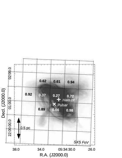
Figure 1 shows the 3\farcm0 3\farcm0 field of view on top of a Chandra image. The scale corresponds to 1.9 pc at a distance of 2.2 kpc (Manchester et al., 2005). This covers a significant fraction of the observed elliptical nebula with a diameter of 2.94.4 pc (Hester, 2008). The SXS was still in the commissioning phase (Tsujimoto et al., 2016), and some instrumental setups were non-nominal. Among them, the gate valve status was most relevant for the result presented here. The valve was closed to keep the Dewar in a vacuum on the ground, which was planned to be opened when we confirmed the initial outgassing had ceased in the spacecraft. This observation was made before this operation. As a result, the attenuation by a 260 m Be window of the gate valve (Eckart et al., 2016) limited the SXS bandpass to above 2 keV, which would otherwise extend down to 0.1 keV.
The instrument had reached the thermal equilibrium by the time of the observation (Fujimoto et al., 2016; Noda et al., 2016). The detector gain was very stable except for the passage of the South Atlantic anomaly. The previous recycle operation of the adiabatic demagnetization refrigerators was started well before the observation at 10:20 on March 24, and the entire observation was within its 48-hour hold time (Shirron et al., 2016). The energy resolution was 4.9 eV measured with the 55Fe calibration source at 5.9 keV for the full width at the half maximum (Porter et al., 2016; Kilbourne et al., 2016; Leutenegger et al., 2016). This superb resolution is not compromised by the extended nature of the Crab nebula for being a non-dispersive spectrometer.
The actual incoming flux measured with the SXS was equivalent to 0.3 Crab in the 2–12 keV band due to the extra attenuation by the gate valve. The net exposure time was 9.7 ks.
2.2 Data Reduction
We started with the cleaned event list produced by the pipeline process version 03.01.005.005 (Angelini et al., 2016). Throughout this paper, we used the HEASoft and CALDB release on 2016 December 22 for the Hitomi collaboration. Further screening against spurious events was applied based on the energy versus pulse rise time. The screening based on the time clustering of multiple events was not applied; it is intended to remove events hitting the out-of-pixel area, but a significant number of false positive detection is expected for high count rate observations like this.
Due to the high count rate, some pixels at the array center suffer dead time (figure 1; Ishisaki et al. (2016)). Still, the observing efficiency of 72% for the entire array is much higher than conventional CCD X-ray spectrometers. For example, Suzaku XIS (Koyama et al., 2007) requires a 1/4 window 0.1 s burst clocking mode to avoid pile-up for a 0.3 Crab source, and the efficiency is only 5%. Details of the dead time and pile-up corrections are described in a separate paper. We only mention here that these effects are much less serious for the SXS than CCDs primarily due to a much faster sampling rate of 12.5 kHz and a continuous readout.
The source spectrum was constructed in the 2–12 keV range at a resolution of 0.5 eV bin-1. Events not contaminated by other events close in time (graded as Hp or Mp; Kelley et al. (2016)) were used for a better energy resolution. All pixels were combined. The redistribution matrix function was generated by including the energy loss processes by escaping electrons and fluorescent X-rays. The half power diameter of the telescope is 1\farcm2 (Okajima et al., 2016). The SXS has only a limited imaging capability, and we do not attempt to perform a spatially-resolved spectroscopic study in this paper. The SXS does have a timing resolution to resolve the 34 ms pulse phase, but we do not attempt a phase-resolved study either as only a small gain in the contrast of thermal emission against the pulse emission is expected; the unpulsed emission of a 90% level of averaged count rate can be extracted at a compensation of 2/3 of the exposure time.
The total number of events in the 2–12 keV range is 7.6105. The background spectrum, which is dominated by the non-X-ray background, was accumulated using the data when the telescope was pointed toward the Earth. The non-X-ray background is known to depend on the strength of the geomagnetic field strength at the position of the spacecraft within a factor of a few. The history of the geomagnetic cut-off rigidity during the Crab observation was taken into consideration to derive the background rate as 8.610-3 s-1 in the 2–12 keV band. This is negligible with 10-4 of the source rate.
3 Analysis
To search for signatures of thermal plasma, we took two approaches. One is to add a thermal plasma emission model, or to multiply a thermal plasma absorption model, upon the best-fit continuum model with an assumed plasma temperature, which we call plasma search (§ 3.1). Here, we assume that the feature is dominant either as emission or absorption. The other is a blind search of emission or absorption lines, in which we test the significance of an addition or a subtraction of a line model upon the best-fit continuum model (§ 3.2). For the spectral fitting, we used the Xspec package version 12.9.0u (Arnaud, 1996). The statistical uncertainties are evaluated at 1 unless otherwise noted.
3.1 Plasma search
3.1.1 Fiducial model
We first constructed the spectral model for the entire energy band. The spectrum was fitted reasonably well with a single power-law model with an interstellar extinction, which we call the fiducial model. Hereafter, all the fitting was performed for unbinned spectra based on the C statistics (Cash, 1979). For the extinction model by cold matter, we used the tbabs model version 2.3.2222See http://pulsar.sternwarte.uni-erlangen.de/wilms/research/tbabs/ for details. (Wilms et al., 2000). We considered the extinction by interstellar gas, molecules, and dust grains with the parameters fixed at the default values of the model except for the total column density. The SXS is capable of resolving the fine structure of absorption edges, which is not included in the model except for O K, Ne K, and Fe L edges. This, however, does not affect the global fitting, as the depths of other edges are shallow for the Crab spectrum.
We calculated the effective area assuming a point-like source at the center of the SXS field. The nebula size is no larger than the point spread function. Figure 2 shows the best-fit model, while table 1 summarizes the best-fit parameters for the extinction column by cold matter (), the power-law photon index (), and the X-ray flux (). The ratio of the data to the model show some broad features, which are attributable to the inaccuracies of the calibration including the mirror Au M and L edge features, the gate valve transmission, the line spread function, ray-tracing modeling accuracies, etc (Okajima et al. in prep.). In this paper, therefore, we constrain ourselves to search for lines that are sufficiently narrow to decouple with these broad systematic uncertainties. This is possible only with high-resolution spectrometers.

| Parameter∗*∗*footnotemark: | Best-fit |
|---|---|
| 1021 cm-2 | 4.6 (4.1–5.0) |
| 2.17 (2.16–2.17) | |
| erg s-1 cm-2††\dagger††\daggerfootnotemark: | 1.722 (1.719–1.728) 10-8 |
| Red-/d.o.f. | 1.34/19996 |
|
∗*∗*footnotemark:
The errors indicate a 1 statistical uncertainty.
††\dagger††\daggerfootnotemark: The absorption-corrected flux at 2–8 keV. |
|
3.1.2 Plasma emission
For the thermal plasma emission, we assumed the optically-thin collisional ionization equilibrium (CIE) plasma model and two non-CIE deviations from it. All the calculations were based on the atomic database ATOMDB (Foster et al., 2012) version 3.0.7. We assumed the solar abundance (Wilms et al., 2000). This gives a conservative upper limit for plasma with a super-solar metalicity when they are searched using metallic lines.
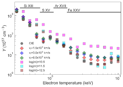
First, we used the apec model (Smith et al., 2001) for the CIE plasma, in which the electron, ion, and ionization temperatures are the same. Neither the bulk motion nor the turbulence broadening was considered, but the thermal broadening was taken into account for the lines. For each varying electron temperature (table 2), we selected the strongest emission line in the 10 non-overlapping 1 keV ranges in the 2–12 keV band. For each selected line, we first fitted the 50 eV range around the line with a power-law model, then added the plasma emission model to set the upper limit of the volume emission measure () of the plasma. Both power-law and plasma emission models were attenuated by an interstellar extinction model of a column density fixed at the fiducial value (table 1). We expect some systematic uncertainty in the value due to incomplete calibration at low energies. The best-fit value in the fiducial model (table 2) tends to be higher than those in the literature (Kaastra et al., 2009; Weisskopf et al., 2010) by 10–30%. A 10% decrease in the value leads to 10% decrease of for the temperature 1 keV. The normalization of the plasma model was allowed to vary both in the positive and negative directions so as not to distort the significance distribution. The result for selected cases is shown in figure 3.
Deviation from the thermal equilibrium is seen in SNR plasmas (Borkowski et al., 2001; Vink, 2012), especially for young SNRs expanding in a low density environment. We considered two types of deviations. One is the non-equilibrium ionization using the nei model (Smith & Hughes, 2010). This code calculates the collisional ionization as a function of the ionization age (), and accounts for the difference between the ionization and electron temperatures. The electron temperature is assumed constant, which is reasonable considering that some SNRs show evidence for the collision-less instantaneous electron heating at the shock (Yamaguchi et al., 2014b). We took the same procedure with the CIE plasma for the values listed in table 2, and derived the upper limit of .
Another non-CIE deviation is that the electron and ion temperatures are different. More massive ions are expected to have a higher temperature than less massive ions and electrons, hence are more thermally broadened before reaching equilibrium. We derived the upper limit of for several values of the ion’s thermal velocity (table 2). In this modeling, the continuum fit was performed over an energy range of the smaller of the two: (3 or 50) eV centered at the line energy , so as to decouple the continuum and line fitting when is large.
| Par | Unit | Description | Total§§\S§§\Sfootnotemark: | Cases§§\S§§\Sfootnotemark: |
| keV | Electron temperature | 21 | 0.1–10 (0.1 dex step) | |
| ∗*∗*footnotemark: | s cm-3 | Ionization age | 8 | 10.0–13.5 (0.5 step) |
| ∗††*\dagger∗††*\daggerfootnotemark: | Thermal broadening of lines | 5 | 0.001, 0.002, 0.005, 0.01, 0.02 | |
| ‡‡\ddagger‡‡\ddaggerfootnotemark: | Shell fraction | 6 | 0.005, 0.01, 0.05, 0.083 (1/12), 0.10, 0.15 | |
|
∗*∗*footnotemark:
The parameter is searched only for the plasma emission (§ 3.1.2).
††\dagger††\daggerfootnotemark: The ion spices has a velocity , thus has a temperature of /, in which is the mass of the ion. In the case of Si and Fe, the cases correspond to 12 MeV and 21 MeV. ‡‡\ddagger‡‡\ddaggerfootnotemark: The value 1/12 is for the self-similar solution (Sedov, 1959), and 0.15 follows preceding work (Seward et al., 2006; Frail et al., 1995). §§\S§§\Sfootnotemark: The adopted parameters (cases) and the total number of cases (total) are shown. |
||||
3.1.3 Plasma absorption
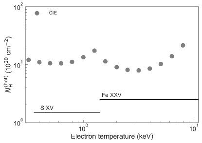
A similar procedure was taken for deriving the upper limit for the absorption column by a thermal plasma. We used the hotabs model (Kallman & Bautista, 2001) and only considered the CIE plasma. At each assumed electron temperature (table 2), we selected the strongest absorption line in the 10 non-overlapping 1 keV ranges in the 2–12 keV band. For each selected line, we first fitted the 50 eV range around the line with a power-law model, then multiplied the plasma absorption model to set the upper limit of the hydrogen-equivalent absorption column () by the plasma. The result is shown in figure 4.
3.1.4 Example in the Fe K band
For the emission, the resultant upper limit of is less constrained for plasma with lower temperatures. At low temperatures, strong lines are at energies below 2 keV, in which the SXS has no sensitivity as the gate valve was not opened. For increasing temperatures above 0.5 keV, S-He, Ar-He, or Fe-He are used to set the limit. The most stringent limit is obtained at the maximum formation temperature (5 keV) of the Fe-He line. For the NEI plasma with a low ionization age (1010.5 s cm-3), He-like Fe ions have not been formed yet, thus the limit is not stringent. Conversely, at an intermediate ionization age (1011.5 s cm-3), Fe is not fully ionized yet, thus Fe-He can give a strong upper limit even for electron temperatures of 10 keV. At 1012.5 s cm-3, the result is the same with the CIE plasma as expected.
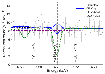
Figure 5 shows a close-up view of the fitting around the Fe-He line for the case of the 3.16 keV electron temperature. Overlaid on the data, models are shown in addition to the best-fit power-law continuum model. Also shown is the expected result by a CCD spectrometer, with which the levels detectable easily with the SXS would be indistinguishable from the continuum emission. This demonstrates the power of an X-ray micro-calorimeter for weak features from extended sources. The expected energy shifts for a bulk velocity of 103 km s-1, or 22.4 eV, are shown. The data quality is quite similar in this range, thus the result is not significantly affected by a possible gain shift (1 eV; Hitomi Collaboration et al. (2016)) or a single bulk velocity shift.
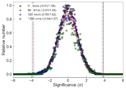
3.2 Blind search
We searched for emission or absorption line features at an arbitrary line energy in the 2–12 keV range. We made trials at 20,000 energies separated by 0.5 eV. The trials were repeated for a fixed line width corresponding to a velocity of 0, 20, 40, 80, 160, 320, 640, and 1280 km s-1. For each set of line energy and width, we fitted the spectrum with a power-law model locally in an energy range 3–20 on both sides of the trial energy . Here, the unit of the fitting range is determined as
| (1) |
in which is the 1 width of the Gaussian core of the detector response (Leutenegger et al., 2016). With this variable fitting range, we can test a wide range of line energy and width. After fixing the best-fit power-law model, we added a Gaussian model allowing both positive and negative amplitudes respectively for emission and absorption lines and refitted in the 0–20 on both sides. The detection significance was evaluated as
| (2) |
in which and are the best-fit and 1 statistical uncertainty of the line normalization in the unit of s-1 cm-2, whereas and are those of the continuum intensity in the unit of s-1 cm-2 keV-1 at the line energy.
Figure 6 shows the distribution of the significance. All are reasonably well fitted by a single Gaussian distribution. We tested several different choices of fitting ranges and confirmed that the overall result does not change. Above a 5 level (0.01 false positives expected for 20,000 trials) of the best-fit Gaussian distribution, no significant detection was found except for (1) several detections of absorption in the 2.0–2.2 keV energy range for a wide velocity range, and (2) a detection of absorption at 9.48 keV for 160 and 320 km s-1. The former is likely due to the inaccurate calibration of the Au M edges of the telescope. For the latter, no instrumental features or strong atomic transitions are known around this energy. However, we do not consider this to be robust as it escapes detection only by changing the fitting ranges.
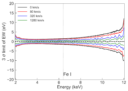
The equivalent width, was derived for every set of the line energy and width along with their 3 statistical uncertainty (figure 7). The 3 limit of EW at 6.4 keV is 2 eV. We would expect the Fe fluorescence line with in which for the Crab’s power-law spectrum (Krolik & Kallman, 1987). and are, respectively, the subtended angle and the H-equivalent column of the fluorescing matter around the incident emission. Assuming and cm-2, which is the measured value in the line of sight inclusive of the ISM (Mori et al., 2004), the expected EW is consistent with the upper limit by the SXS.
4 Discussion
In § 4.1, we convert the upper limit of or with the SXS into that of the plasma density () by making several assumptions. In § 4.2, we re-evaluate the data by other methods in the literature under the same assumptions to assemble the most stringent upper limit of for various ranges of the parameters. In § 4.3, we perform a HD calculation for some SN models and verify that the searched parameter ranges are reasonable. In § 4.4, we compare the HD result with observed limits.
4.1 Constraints on the plasma density with SXS
For converting the upper limits of and of the thermal plasma into that of the X-ray emitting plasma density (), we assume the plasma is uniform in a spherically symmetric shell in a range of to from the center. We assumed several shell fraction () values (table 2). For simplicity, the electron and ion densities are the same, and all ions are hydrogen. This gives a conservative upper limit for the plasma mass.
We first use the upper limit of the plasma emission. The density is , in which is the observed emitting volume. Some selected cases are shown in figure 8 (thick solid and dashed curves). If the SXS square field of view with 3\farcm0 covers the entire shell at 1\farcm3, . If the field is entirely contained in the shell at 2\farcm1, should be replaced with , in which is the distance to the source. These approximations at the two ends make a smooth transition.
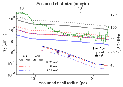
Here, we made a correction for the reduced effective area for the extended structure of the shell. As increases within the SXS field of view, the effective area averaged over the view decreases as more photons are close to the field edges. This effect is small in the case of the Crab because the central pixels suffer dead time due to the high count rate (figure 1). In fact, a slightly extended structure up to 1\farcm2 has a larger effective area than a point-like distribution. As increase beyond the field, the emission within the field becomes closer to a flat distribution, and the reduction of the effective area levels off (figure 8; green data and dashed curve).
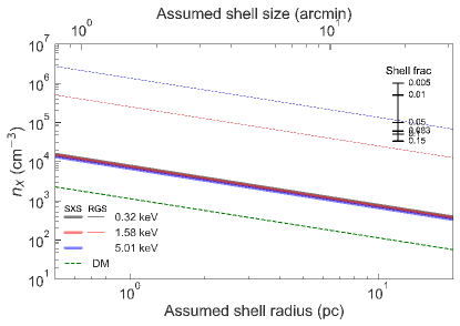
Next, we convert the upper limits by the extinction column to the density with , which is shown in figure 9 (thick lines). We assume that the absorption feature is superposed on a point-like continuum source, thus no correction was made for the extended structure.
4.2 Results with other techniques
We compare the results with the previous work using three different techniques. First, Seward et al. (2006) used the Advanced CCD Imaging Spectrometer (ACIS; Garmire et al. (2003)) onboard the Chandra X-ray Observatory (Weisskopf et al., 2002) with an unprecedented imaging resolution, and derived the upper limit of the thermal emission assuming that it would be detectable if it has a 0.1 times surface brightness of the observed halo emission attributable to the dust scattering. We re-evaluated their raw data (their figure 5) under the same assumptions with SXS (figure 8; thin solid and dashed curves). No ACIS limit was obtained below \arcmin due to the extreme brightness of the PWN. Beyond \arcmin, at which there is no ACIS measurement, we used the upper limit at 18\arcmin. For the ACIS limits, a more stringent limit is obtained for the NEI case with a low ionization age (1010.5 s cm-3) than the CIE case with the same temperature. This is because the Fe L series lines are enhanced for such NEI plasmas and the ACIS is sensitive also at 2 keV unlike the SXS with the gate valve closed.
Second, Kaastra et al. (2009) presented the Crab spectrum using the Reflecting Grating Spectrometer (RGS; den Herder et al. (2001)) onboard the XMM-Newton Observatory (Jansen et al., 2001) observatory. Upon the non-thermal emission of the PWN, they reported a detection of the absorption feature by the O-He and O-Ly lines respectively at 0.58 and 0.65 keV with a similar equivalent width of 0.2 eV assuming that the lines are narrow. The former was also confirmed in the Chandra Low Energy Transmission Grating data. However, these absorption lines are often seen in the spectra of Galactic X-ray binaries (e.g., Yao & Wang (2006)), which is attributed to the hot gas in the interstellar medium with a temperature of a few MK. Adopting the value by Sakai et al. (2014), the expected column density by such a gas to the Crab is 81018 cm-2, which is non-negligible. We therefore consider that the values measured with RGS are an upper limit for the plasma around the Crab. Using the same assumptions with SXS, we re-evaluated the RGS limit (thin lines in figure 9).
Third, the dispersion measure from the Crab pulsar reflects the column density of ionized gas along the line of sight. This includes not only the undetected thermal plasma around the Crab but also the hot and warm interstellar gas. Lundgren et al. (1995) derived a measure 1.81020 cm-2, which converts to another density limit (dashed line in figure 9).
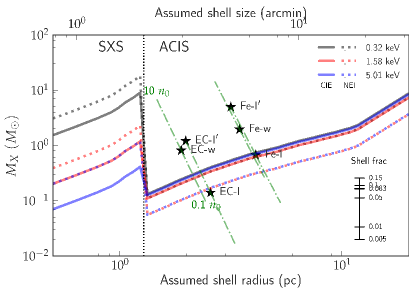
We now have the upper limit on for several sets of , , and by assembling the lowest values among various methods (re)-evaluated under the same assumptions. We convert the limit to that of the total X-ray emitting mass , where is the proton mass and is the total emitting volume for an assumed shell size and fraction. The resultant limit is shown in Figure 10. The most stringent limit is given by the emission search either by ACIS or SXS. The SXS result complements the ACIS result at pc, and the two give an upper limit of 1 for the X-ray emitting plasma at any shell radius. The exception is for the low plasma temperature below 1 keV, for which the SXS with the closed gate valve yields a less constraining limit.
4.3 HD calculation
We performed a HD calculation to verify that the searched parameter ranges (table 2) are reasonable and to confirm if there are any SN models consistent with the observed limit. We used the CR-hydro-NEI code (Lee et al. (2014) and references therein), which calculates time-dependent, non-equilibrium plasma in one dimension. At the forward shock, the kinetic energy is thermalized independently for each species, thus the temperature is proportional to the mass of the species. The plasma is then thermally relaxed by the Coulomb interaction. No collissionless shocks are included. Energy loss by radiation is included, while that by cosmic rays is omitted.
We considered two SN explosion models under two circumstellar environments (table 3) as representatives. The former two are (a) the Fe-core collapse SN by a red super-giant progenitor with the initial explosion energy erg and the ejecta mass (Patnaude et al., 2015), and (b) the electron capture (EC) SN by a super AGB progenitor with erg and (Moriya et al., 2014). The latter two are (1) the uniform density cm-3 and (2) the density profile by the progenitor wind: , in which the mass loss rate yr-1 and the wind velocity km s-1 (Moriya et al., 2014). In the wind density parameter (Chugai & Danziger, 1994), g cm-1.
The 22 models are labeled as (a-1) Fe-I, (a-2) Fe-w, (b-1) EC-I, and (b-2) EC-w. For Fe-I and EC-I models, we also calculated an elevated ISM density of cm-3 (respectively labeled as Fe-I′ and EC-I′). For all these models, we assumed the power () of the unshocked ejecta density as a function of velocity to be 9 (Fransson et al., 1996). Only for the model EC-w, we calculated with to see the effect of this parameter (labeled as EC-w′′).
| Label | Fe-I | Fe-I′ | Fe-w | EC-I | EC-I′ | EC-w | EC-w′′ |
|---|---|---|---|---|---|---|---|
| (SN setup) | |||||||
| SN explosion | Fe | Fe | Fe | EC | EC | EC | EC |
| (1051 erg) | 1.21 | 1.21 | 1.21 | 0.15 | 0.15 | 0.15 | 0.15 |
| () | 12.1 | 12.1 | 12.1 | 4.36 | 4.36 | 4.36 | 4.36 |
| 9 | 9 | 9 | 9 | 9 | 9 | 7 | |
| Environment | ISM | ISM | wind | ISM | ISM | wind | wind |
| (cm-3) | 0.1 | 1.0 | — | 0.1 | 1.0 | — | — |
| (1014 g cm-1) | — | — | 3.2 | — | — | 3.2 | 3.2 |
| (SNR outcome) | |||||||
| (pc) | 4.6 | 3.6 | 4.3 | 2.9 | 2.2 | 2.3 | 2.6 |
| (pc) | 4.1 | 3.2 | 3.5 | 2.6 | 2.0 | 1.9 | 2.0 |
| (pc) | 3.8 | 2.9 | 3.3 | 2.4 | 1.8 | 1.8 | 1.9 |
| (103 km s-1) | 3.1 | 2.4 | 3.7 | 2.0 | 1.5 | 2.0 | 2.1 |
| ∗*∗*footnotemark: (103 km s-1) | 1.4 | 1.2 | 0.51 | 0.88 | 0.68 | 0.29 | 0.39 |
| () | 1.4 | 6.6 | 2.0 | 0.35 | 1.6 | 1.1 | 1.2 |
| () | 1.8 | 7.0 | 4.1 | 0.42 | 2.2 | 2.2 | 1.3 |
| —— derived values —— | |||||||
| 0.07 | 0.07 | 0.04 | 0.06 | 0.09 | 0.04 | 0.07 | |
| (keV) | 9.4 | 5.7 | 13 | 3.8 | 2.2 | 4.0 | 4.1 |
| () | 10 | 5.1 | 8.0 | 3.9 | 2.2 | 2.2 | 3.0 |
| —— absorbed X-ray flux weighted average —— | |||||||
| (keV) | 1.0 | 1.6 | 0.51 | 0.71 | 0.95 | 0.74 | 0.51 |
| (keV) | 130 | 26 | 50 | 57 | 4.0 | 62 | 90 |
| (1011 cm s-1) | 0.21 | 1.5 | 9.9 | 0.22 | 1.59 | 11.8 | 10.2 |
| () | 0.67 | 5.0 | 2.0 | 0.14 | 1.2 | 0.81 | 1.1 |
|
∗*∗*footnotemark:
Velocity with respect to the ejecta.
|
|||||||
Table 3 summarizes the SN setup stated above and the SNR outcome at an age of 962 yr, which includes the radius of the forward shock (FS), contact discontinuity (CD), and reverse shock (RS) (, , and ), the velocity of the forward and reverse shocks ( and ), the mass between CD and FS () and that between RS and CD (). The two masses represent the shocked ISM and ejecta, respectively. The radius is close to the observed size of the optical photo-ionized nebula, and the radii and velocities match reasonably well with analytical approaches (Chevalier, 1982; Truelove & McKee, 1999) within 10%, which validates our calculation. The RS radius is larger than the X-ray emitting synchrotron nebula, which justifies that our calculation does not include the interaction with it.
From these, we calculated as a proxy for the shell fraction, as a proxy for the electron temperature after Coulomb relaxation, in which is the mean molecular weight, and the unshocked ejecta mass . We also derived the average of the electron and Fe temperatures ( and ) and the ionization age () weighted over the absorbed X-ray flux. The X-ray emitting mass () was estimated by integrating the mass with a temperature in excess of .
The searched ranges of all parameters (table 2) encompass the HD result for all models. The electron temperature is expected between and ; the former is the highest for thermalizing all the kinetic energy instantaneously, while the latter is the lowest for starting the Coulomb relaxation without collision-less heating. The averaged Fe temperature is sufficiently low to consider that the line is relatively narrow; the thermal broadening by this is 32 eV at 6.7 keV for =130 keV. The ionization age () ranges over two orders from 1010 to 1012 cm-3 s-1 depending on the pre-explosion environment, where the wind density cases result in higher values than the ISM density cases.
4.4 Comparison with observed limits
Finally, we compare the HD results with the observation in figure 10. For the radius and the X-ray plasma mass, we plotted (, ) in table 3. The shell size by the models () is larger than 1.3 pc, where we have a stringent limit on with the observations. The HD results depend on the choice of the parameters in the SN setup (, , or , and ; table 3). We can estimate in which direction the model points move in the plot when these parameters are changed.
First, the two parameters and are known to be correlated in type II SNe. Our two SN models are in line with the relation by Pejcha & Prieto (2015). Therefore, the model points move roughly in the direction of the lines connecting the EC-I and Fe-I models, or the EC-w and Fe-w models. For a fixed explosion energy of 1.211051 erg for our Fe model, a plausible range of is 12–32 (Pejcha & Prieto, 2015), thus our model is close to the lower bound. Second, for , the points move in parallel with the lines connecting Fe-I and Fe-I′ or EC-I and EC-I′. This should be the same for in the wind environment case. Third, for , there is little difference between the result of the model Fe-w and Fe-w′′, so we consider that this parameter does not affect the result very much. In terms of the comparison with the observation limit, or is the most important factor.
Although the small observed mass of the Crab is argued to rule out an Fe core collapse SN for its origin (Seward et al., 2006), we consider that this does not simply hold. Our models illustrate that such a small mass can be reproduced if an Fe core collapse SN explosion takes place in a sufficiently low density environment with the ISM density 0.03 cm-3 (Fe-I) or the wind density parameter g cm-1 (Fe-w). In such a case, a large fraction of the ejecta mass is unshocked (table 3) and escapes from detection. Some of the unshocked ejecta may be visible when they are photo-ionized by the emission from the PWN to a 103 K gas (Fesen et al., 1997) or a 104 K gas (Sollerman et al., 2000).
We argue that both the Fe and EC models still hold to be compatible with the observed mass limits. In either case, it is strongly preferred that the pre-explosion environment is low in density; i.e., cm-3 (EC-I) or cm-3 (Fe-I) for the ISM environment or g cm-1 for the wind environment (both Fe-w and EC-w). For the latter, a large value (e.g., g cm-1; Smith (2013)), which is an idea to explain the initial brightness of SN 1054, is not favored. In fact, such a low density environment is suggested by observations. At the position of the Crab, which is off-plane in the anti-Galactic center direction, the ISM density is 0.3 cm-3 by a Galactic model (Ferrière, 1998). Wallace et al. (1999) further claimed the presence of a bubble around the Crab based on an H I mapping with a density lower than the surroundings. Our result suggests that SN 1054 took place in such a low environment and the wind environment by its progenitor of a low wind density value.
5 Conclusion
We utilized the SXS calibration data of the Crab nebula in 2–12 keV to set an upper limit to the thermal plasma density by spectroscopically searching for emission or absorption features in the Crab spectrum. No significant emission or absorption features were found in both the plasma and the blind searches.
Along with the data in the literature, we evaluated the result under the same assumptions to derive the X-ray plasma mass limit to be for a wide range of assumed shell radii () and plasma temperatures (). The SXS sets a new limit in 1.3 pc for keV. We also performed HD simulations of the Crab SNR for two SN explosion models under two pre-explosion environments. Both SN models are compatible with the observed limits when the pre-explosion environment has a low density of 0.03 cm-3 (Fe model) or 0.1 cm-3 (EC model) for the uniform density, or 1014 g cm-1 ( yr-1 for 20 km s-1) for the wind density parameter in the wind environment.
A low energy explosion is favored based on the abundance, initial light curve, and nebular size studies (MacAlpine & Satterfield, 2008; Moriya et al., 2014; Yang & Chevalier, 2015). We believe that a positive detection of thermal plasma, in particular with lines, is key to distinguishing the Fe and EC models. It is worth noting that the observed limit is close to the model predictions. We now know the high potential of a spectroscopic search with the SXS, and may expect a detection of the thermal feature by placing the SXS field center at several offset positions. With a 10 ks snapshot at four different positions at the radius of EC-I and Fe-I models (respectively 2.6 and 4.1 pc), an upper limit lower than that with ACIS by a factor of a few is expected (figure 8).
This was exactly what was planned next. If it were not for the loss of the spacecraft estimated to have happened at 1:42 UT on 2016 March 26, a series of the offset Crab observations should have started 8 hours later for calibration purposes, which should have been followed by the gate valve open to allow access down to 0.1 keV. The 8 hours now turned to be many years, but we should be back as early as possible.
Author contributions
M. Tsujimoto led this study in data analysis and writing drafts. He also contributed to the SXS hardware design, fabrication, integration and tests, launch campaign, in-orbit operation, and calibration. S.-H. Lee performed the hydro calculations and its interpretations for this paper. K. Mori and H. Yamaguchi contributed to discussion on SNRs. They also made hardware and software contributions to the Hitomi satellite. N. Tominaga and T. J. Moriya gave critical comments on SNe. T. Sato worked for the telescope response for the data analysis and calibration. C. de Vries led the filter wheel of the SXS, which gave the only pixel-to-pixel gain reference of this spectrometer in the orbit. R. Iizuka contributed to the testing and calibration of the telescope, and the operation of the SXS. A. R. Foster and T. Kallman helped with the plasma models. M. Ishida, R. F. Mushotzky, A. Bamba, R. Petre, B. J. Williams, S. Safi-Harb, A. C. Fabian, C. Pinto, L. C. Gallo, E. M. Cackett, J. Kaastra, M. Ozaki, J. P. Hughes, and D. McCammon improved the draft.
We appreciate all people contributed to the SXS, which made this work possible. We also thank Toru Misawa in Shinshu University for discussing the C IV feature.
We thank the support from the JSPS Core-to-Core Program. We acknowledge all the JAXA members who have contributed to the ASTRO-H (Hitomi) project. All U.S. members gratefully acknowledge support through the NASA Science Mission Directorate. Stanford and SLAC members acknowledge support via DoE contract to SLAC National Accelerator Laboratory DE-AC3-76SF00515. Part of this work was performed under the auspices of the U.S. DoE by LLNL under Contract DE-AC52-07NA27344. Support from the European Space Agency is gratefully acknowledged. French members acknowledge support from CNES, the Centre National d’Études Spatiales. SRON is supported by NWO, the Netherlands Organization for Scientific Research. Swiss team acknowledges support of the Swiss Secretariat for Education, Research and Innovation (SERI). The Canadian Space Agency is acknowledged for the support of Canadian members. We acknowledge support from JSPS/MEXT KAKENHI grant numbers 15H00773, 15H00785, 15H02090, 15H03639, 15H05438, 15K05107, 15K17610, 15K17657, 16H00949, 16H06342, 16K05295, 16K05300, 16K13787, 16K17672, 16K17673, 21659292, 23340055, 23340071, 23540280, 24105007, 24540232, 25105516, 25109004, 25247028, 25287042, 25400236, 25800119, 26109506, 26220703, 26400228, 26610047, 26800102, JP15H02070, JP15H03641, JP15H03642, JP15H03642, JP15H06896, JP16H03983, JP16K05296, JP16K05309, JP16K17667, and 16K05296. The following NASA grants are acknowledged: NNX15AC76G, NNX15AE16G, NNX15AK71G, NNX15AU54G, NNX15AW94G, and NNG15PP48P to Eureka Scientific. H. Akamatsu acknowledges support of NWO via Veni grant. C. Done acknowledges STFC funding under grant ST/L00075X/1. A. Fabian and C. Pinto acknowledge ERC Advanced Grant 340442. P. Gandhi acknowledges JAXA International Top Young Fellowship and UK Science and Technology Funding Council (STFC) grant ST/J003697/2. Y. Ichinohe, K. Nobukawa, H. Seta, and T. Sato are supported by the Research Fellow of JSPS for Young Scientists. N. Kawai is supported by the Grant-in-Aid for Scientific Research on Innovative Areas “New Developments in Astrophysics Through Multi-Messenger Observations of Gravitational Wave Sources”. S. Kitamoto is partially supported by the MEXT Supported Program for the Strategic Research Foundation at Private Universities, 2014-2018. B. McNamara and S. Safi-Harb acknowledge support from NSERC. T. Dotani, T. Takahashi, T. Tamagawa, M. Tsujimoto and Y. Uchiyama acknowledge support from the Grant-in-Aid for Scientific Research on Innovative Areas “Nuclear Matter in Neutron Stars Investigated by Experiments and Astronomical Observations”. N. Werner is supported by the Lendület LP2016-11 grant from the Hungarian Academy of Sciences. D. Wilkins is supported by NASA through Einstein Fellowship grant number PF6-170160, awarded by the Chandra X-ray Center, operated by the Smithsonian Astrophysical Observatory for NASA under contract NAS8-03060.
We thank contributions by many companies, including in particular, NEC, Mitsubishi Heavy Industries, Sumitomo Heavy Industries, and Japan Aviation Electronics Industry. Finally, we acknowledge strong support from the following engineers. JAXA/ISAS: Chris Baluta, Nobutaka Bando, Atsushi Harayama, Kazuyuki Hirose, Kosei Ishimura, Naoko Iwata, Taro Kawano, Shigeo Kawasaki, Kenji Minesugi, Chikara Natsukari, Hiroyuki Ogawa, Mina Ogawa, Masayuki Ohta, Tsuyoshi Okazaki, Shin-ichiro Sakai, Yasuko Shibano, Maki Shida, Takanobu Shimada, Atsushi Wada, Takahiro Yamada; JAXA/TKSC: Atsushi Okamoto, Yoichi Sato, Keisuke Shinozaki, Hiroyuki Sugita; Chubu U: Yoshiharu Namba; Ehime U: Keiji Ogi; Kochi U of Technology: Tatsuro Kosaka; Miyazaki U: Yusuke Nishioka; Nagoya U: Housei Nagano; NASA/GSFC: Thomas Bialas, Kevin Boyce, Edgar Canavan, Michael DiPirro, Mark Kimball, Candace Masters, Daniel Mcguinness, Joseph Miko, Theodore Muench, James Pontius, Peter Shirron, Cynthia Simmons, Gary Sneiderman, Tomomi Watanabe; ADNET Systems: Michael Witthoeft, Kristin Rutkowski, Robert S. Hill, Joseph Eggen; Wyle Information Systems: Andrew Sargent, Michael Dutka; Noqsi Aerospace Ltd: John Doty; Stanford U/KIPAC: Makoto Asai, Kirk Gilmore; ESA (Netherlands): Chris Jewell; SRON: Daniel Haas, Martin Frericks, Philippe Laubert, Paul Lowes; U of Geneva: Philipp Azzarello; CSA: Alex Koujelev, Franco Moroso.
References
- Angelini et al. (2016) Angelini, L., Terada, Y., Loewenstein, M., et al. 2016, in Proc. SPIE, Vol. 9905, Society of Photo-Optical Instrumentation Engineers (SPIE) Conference Series, 990514
- Arnaud (1996) Arnaud, K. A. 1996, in Astronomical Society of the Pacific Conference Series, Vol. 101, Astronomical Data Analysis Software and Systems V, ed. G. H. Jacoby & J. Barnes, 17
- Baade & Zwicky (1934) Baade, W. & Zwicky, F. 1934, Proceedings of the National Academy of Science, 20, 254
- Bamba et al. (2010) Bamba, A., Mori, K., & Shibata, S. 2010, ApJ, 709, 507
- Borkowski et al. (2001) Borkowski, K. J., Lyerly, W. J., & Reynolds, S. P. 2001, ApJ, 548, 820
- Cash (1979) Cash, W. 1979, ApJ, 228, 939
- Chevalier (1977) Chevalier, R. A. 1977, in Astrophysics and Space Science Library, Vol. 66, Supernovae, ed. D. N. Schramm, 53
- Chevalier (1982) Chevalier, R. A. 1982, ApJ, 258, 790
- Chugai & Danziger (1994) Chugai, N. N. & Danziger, I. J. 1994, MNRAS, 268, 173
- Davidson & Fesen (1985) Davidson, K. & Fesen, R. A. 1985, ARA&A, 23, 119
- den Herder et al. (2001) den Herder, J. W., Brinkman, A. C., Kahn, S. M., et al. 2001, A&A, 365, L7
- Eckart et al. (2016) Eckart, M. E., Adams, J. S., Boyce, K. R., et al. 2016, in Proc. SPIE, Vol. 9905, Society of Photo-Optical Instrumentation Engineers (SPIE) Conference Series, 99053W
- Ferrand & Safi-Harb (2012) Ferrand, G. & Safi-Harb, S. 2012, Advances in Space Research, 49, 1313
- Ferrière (1998) Ferrière, K. 1998, ApJ, 497, 759
- Fesen et al. (1997) Fesen, R. A., Shull, J. M., & Hurford, A. P. 1997, AJ, 113, 354
- Foster et al. (2012) Foster, A. R., Ji, L., Smith, R. K., & Brickhouse, N. S. 2012, ApJ, 756, 128
- Frail et al. (1995) Frail, D. A., Kassim, N. E., Cornwell, T. J., & Goss, W. M. 1995, ApJ, 454, L129
- Fransson et al. (1996) Fransson, C., Lundqvist, P., & Chevalier, R. A. 1996, ApJ, 461, 993
- Fujimoto et al. (2016) Fujimoto, R., Takei, Y., Mitsuda, K., et al. 2016, in Proc. SPIE, Vol. 9905, Society of Photo-Optical Instrumentation Engineers (SPIE) Conference Series, 99053S
- Garmire et al. (2003) Garmire, G. P., Bautz, M. W., Ford, P. G., Nousek, J. A., & Ricker, Jr., G. R. 2003, in Society of Photo-Optical Instrumentation Engineers (SPIE) Conference Series, Vol. 4851, Society of Photo-Optical Instrumentation Engineers (SPIE) Conference Series, ed. J. E. Truemper & H. D. Tananbaum, 28–44
- Hester (2008) Hester, J. J. 2008, ARA&A, 46, 127
- Hitomi Collaboration et al. (2016) Hitomi Collaboration, Aharonian, F., Akamatsu, H., et al. 2016, Nature, 535, 117
- Hughes et al. (1995) Hughes, J. P., Hayashi, I., Helfand, D., et al. 1995, ApJ, 444, L81
- Ishisaki et al. (2016) Ishisaki, Y., Yamada, S., Seta, H., et al. 2016, in Proc. SPIE, Vol. 9905, Society of Photo-Optical Instrumentation Engineers (SPIE) Conference Series, 99053T
- Jahoda et al. (2006) Jahoda, K., Markwardt, C. B., Radeva, Y., et al. 2006, ApJS, 163, 401
- Janka et al. (2008) Janka, H.-T., Müller, B., Kitaura, F. S., & Buras, R. 2008, A&A, 485, 199
- Jansen et al. (2001) Jansen, F., Lumb, D., Altieri, B., et al. 2001, A&A, 365, L1
- Kaastra et al. (2009) Kaastra, J. S., de Vries, C. P., Costantini, E., & den Herder, J. W. A. 2009, A&A, 497, 291
- Kallman & Bautista (2001) Kallman, T. & Bautista, M. 2001, ApJS, 133, 221
- Kargaltsev et al. (2012) Kargaltsev, O., Durant, M., Pavlov, G. G., & Garmire, G. 2012, ApJS, 201, 37
- Kelley et al. (2016) Kelley, R. L., Akamatsu, H., Azzarello, P., et al. 2016, in Proc. SPIE, Vol. 9905, Society of Photo-Optical Instrumentation Engineers (SPIE) Conference Series, 99050V
- Kilbourne et al. (2016) Kilbourne, C. A., Adams, J. S., Brekosky, R. P., et al. 2016, in Proc. SPIE, Vol. 9905, Society of Photo-Optical Instrumentation Engineers (SPIE) Conference Series, 99053L
- Kirsch et al. (2005) Kirsch, M. G., Briel, U. G., Burrows, D., et al. 2005, in Proc. SPIE, Vol. 5898, UV, X-Ray, and Gamma-Ray Space Instrumentation for Astronomy XIV, ed. O. H. W. Siegmund, 22–33
- Kitaura et al. (2006) Kitaura, F. S., Janka, H.-T., & Hillebrandt, W. 2006, A&A, 450, 345
- Koyama et al. (2007) Koyama, K., Tsunemi, H., Dotani, T., et al. 2007, PASJ, 59, 23
- Krolik & Kallman (1987) Krolik, J. H. & Kallman, T. R. 1987, ApJ, 320, L5
- Lee et al. (2014) Lee, S.-H., Patnaude, D. J., Ellison, D. C., Nagataki, S., & Slane, P. O. 2014, ApJ, 791, 97
- Leutenegger et al. (2016) Leutenegger, M. A., Audard, M., Boyce, K. R., et al. 2016, in Proc. SPIE, Vol. 9905, Society of Photo-Optical Instrumentation Engineers (SPIE) Conference Series, 99053U
- Lobanov et al. (2011) Lobanov, A. P., Horns, D., & Muxlow, T. W. B. 2011, A&A, 533, A10
- Lovelace et al. (1968) Lovelace, R. B. E., Sutton, J. M., & Craft, H. D. 1968, IAU Circ., 2113
- Lundgren et al. (1995) Lundgren, S. C., Cordes, J. M., Ulmer, M., et al. 1995, ApJ, 453, 433
- Lundmark (1921) Lundmark, K. 1921, PASP, 33, 225
- MacAlpine & Satterfield (2008) MacAlpine, G. M. & Satterfield, T. J. 2008, AJ, 136, 2152
- Madsen et al. (2015) Madsen, K. K., Reynolds, S., Harrison, F., et al. 2015, ApJ, 801, 66
- Manchester et al. (2005) Manchester, R. N., Hobbs, G. B., Teoh, A., & Hobbs, M. 2005, AJ, 129, 1993
- Mattana et al. (2009) Mattana, F., Falanga, M., Götz, D., et al. 2009, ApJ, 694, 12
- Mauche & Gorenstein (1985) Mauche, C. W. & Gorenstein, P. 1985, in The Crab Nebula and Related Supernova Remnants, ed. M. C. Kafatos & R. B. C. Henry, 81–88
- Mori et al. (2004) Mori, K., Burrows, D. N., Hester, J. J., et al. 2004, ApJ, 609, 186
- Moriya et al. (2014) Moriya, T. J., Tominaga, N., Langer, N., et al. 2014, A&A, 569, A57
- Ng & Romani (2008) Ng, C.-Y. & Romani, R. W. 2008, ApJ, 673, 411
- Noda et al. (2016) Noda, H., Mitsuda, K., Okamoto, A., et al. 2016, in Proc. SPIE, Vol. 9905, Society of Photo-Optical Instrumentation Engineers (SPIE) Conference Series, 99053R
- Nomoto et al. (1982) Nomoto, K., Sugimoto, D., Sparks, W. M., et al. 1982, Nature, 299, 803
- Okajima et al. (2016) Okajima, T., Soong, Y., Serlemitsos, P., et al. 2016, in Proc. SPIE, Vol. 9905, Society of Photo-Optical Instrumentation Engineers (SPIE) Conference Series, 99050Z
- Patnaude et al. (2015) Patnaude, D. J., Lee, S.-H., Slane, P. O., et al. 2015, ApJ, 803, 101
- Pejcha & Prieto (2015) Pejcha, O. & Prieto, J. L. 2015, ApJ, 806, 225
- Porter et al. (2016) Porter, F. S., Boyce, K. R., Chiao, M. P., et al. 2016, in Proc. SPIE, Vol. 9905, Society of Photo-Optical Instrumentation Engineers (SPIE) Conference Series, 99050W
- Possenti et al. (2002) Possenti, A., Cerutti, R., Colpi, M., & Mereghetti, S. 2002, A&A, 387, 993
- Predehl & Schmitt (1995) Predehl, P. & Schmitt, J. H. M. M. 1995, A&A, 293, 889
- Rudie et al. (2008) Rudie, G. C., Fesen, R. A., & Yamada, T. 2008, MNRAS, 384, 1200
- Sakai et al. (2014) Sakai, K., Yao, Y., Mitsuda, K., et al. 2014, PASJ, 66, 83
- Savitzky & Golay (1964) Savitzky, A. & Golay, M. J. E. 1964, Anal. Chem., 36(8), 1627
- Sedov (1959) Sedov, L. I. 1959, Similarity and Dimensional Methods in Mechanics
- Seward et al. (2006) Seward, F. D., Tucker, W. H., & Fesen, R. A. 2006, ApJ, 652, 1277
- Shirron et al. (2016) Shirron, P. J., Kimball, M. O., James, B. L., et al. 2016, in Proc. SPIE, Vol. 9905, Society of Photo-Optical Instrumentation Engineers (SPIE) Conference Series, 99053O
- Smith (2013) Smith, N. 2013, MNRAS, 434, 102
- Smith et al. (2001) Smith, R. K., Brickhouse, N. S., Liedahl, D. A., & Raymond, J. C. 2001, ApJ, 556, L91
- Smith & Hughes (2010) Smith, R. K. & Hughes, J. P. 2010, ApJ, 718, 583
- Sollerman et al. (2001) Sollerman, J., Kozma, C., & Lundqvist, P. 2001, A&A, 366, 197
- Sollerman et al. (2000) Sollerman, J., Lundqvist, P., Lindler, D., et al. 2000, ApJ, 537, 861
- Staelin & Reifenstein (1968) Staelin, D. H. & Reifenstein, III, E. C. 1968, Science, 162, 1481
- Stephenson & Green (2002) Stephenson, F. R. & Green, D. A. 2002, Historical supernovae and their remnants, by F. Richard Stephenson and David A. Green. International series in astronomy and astrophysics, vol. 5. Oxford: Clarendon Press, 2002, ISBN 0198507666, 5
- Takahashi et al. (2016) Takahashi, T., Kokubun, M., Mitsuda, K., & et al. 2016, in Proc. SPIE, Vol. 9905, Society of Photo-Optical Instrumentation Engineers (SPIE) Conference Series, 99050U
- Terada et al. (2008) Terada, Y., Enoto, T., Miyawaki, R., et al. 2008, PASJ, 60, S25
- Tominaga et al. (2013) Tominaga, N., Blinnikov, S. I., & Nomoto, K. 2013, ApJ, 771, L12
- Truelove & McKee (1999) Truelove, J. K. & McKee, C. F. 1999, ApJS, 120, 299
- Tsujimoto et al. (2016) Tsujimoto, M., Mitsuda, K., Kelley, R. L., et al. 2016, in Proc. SPIE, Vol. 9905, Society of Photo-Optical Instrumentation Engineers (SPIE) Conference Series, 99050Y
- Tziamtzis et al. (2009) Tziamtzis, A., Schirmer, M., Lundqvist, P., & Sollerman, J. 2009, A&A, 497, 167
- Vink (2012) Vink, J. 2012, A&A Rev., 20, 49
- Wallace et al. (1999) Wallace, B. J., Landecker, T. L., Kalberla, P. M. W., & Taylor, A. R. 1999, ApJS, 124, 181
- Weisskopf et al. (2002) Weisskopf, M. C., Brinkman, B., Canizares, C., et al. 2002, PASP, 114, 1
- Weisskopf et al. (2010) Weisskopf, M. C., Guainazzi, M., Jahoda, K., et al. 2010, ApJ, 713, 912
- Wilms et al. (2000) Wilms, J., Allen, A., & McCray, R. 2000, ApJ, 542, 914
- Yamaguchi et al. (2014a) Yamaguchi, H., Badenes, C., Petre, R., et al. 2014a, ApJ, 785, L27
- Yamaguchi et al. (2014b) Yamaguchi, H., Eriksen, K. A., Badenes, C., et al. 2014b, ApJ, 780, 136
- Yang & Chevalier (2015) Yang, H. & Chevalier, R. A. 2015, ApJ, 806, 153
- Yao & Wang (2006) Yao, Y. & Wang, Q. D. 2006, ApJ, 641, 930