Fairer and more accurate, but for whom?

Abstract.

Complex statistical machine learning models are increasingly being used or considered for use in high-stakes decision-making pipelines in domains such as financial services, health care, criminal justice and human services. These models are often investigated as possible improvements over more classical tools such as regression models or human judgement. While the modeling approach may be new, the practice of using some form of risk assessment to inform decisions is not.

When determining whether a new model should be adopted, it is therefore essential to be able to compare the proposed model to the existing approach across a range of task-relevant accuracy and fairness metrics. Looking at overall performance metrics, however, may be misleading. Even when two models have comparable overall performance, they may nevertheless disagree in their classifications on a considerable fraction of cases.

In this paper we introduce a model comparison framework for automatically identifying subgroups in which the differences between models are most pronounced. Our primary focus is on identifying subgroups where the models differ in terms of fairness-related quantities such as racial or gender disparities. We present experimental results from a recidivism prediction task and a hypothetical lending example.

1. Introduction

Actuarial and clinical assessments of risk have long been mainstays of decision making in domains such as criminal justice, health care and human services. Within the criminal justice system, for instance, recidivism prediction instruments and judicial discretion commonly enter into decisions concerning bail, parole and sentencing. In these high-stakes settings, decisions made based on erroneous predictions can have a direct adverse impact on individuals’ lives. Institutions are therefore continually seeking to improve the accuracy of their risk predictions, and many are turning to proprietary commercial tools and more complex “black-box” prediction models in pursuit of accuracy gains.

When determining whether to replace or augment an existing risk assessment method, it is important to compare the proposed model to the existing approach across a range of task-relevant accuracy and fairness metrics. As we will demonstrate, a comparison that looks only at overall performance can present an incomplete and potentially misleading picture.

A motivating example. In May 2016 an investigative journalism team at ProPublica released a report (Angwin et al., 2016b) on a proprietary recidivism prediction instrument called COMPAS(Northpointe, 2010), developed by Northpointe Inc. The data set (Angwin et al., 2016a) released as part of this report contains COMPAS decile scores, 2-year recidivism outcomes and a number of demographic and crime-related variables for defendants scored as part of pre-trial proceedings in Broward County, Florida. In particular, the data set contains information on the number of prior offenses (hereon denoted Priors) for each defendant. Since criminal history is itself a good predictor of future recidivism, it is reasonable to suppose that before COMPAS was introduced, judges could have based their risk assessments on Priors instead. Our question is thus: Does COMPAS produce more accurate (and/or equitable) predictions of recidivism than Priors alone?

The table below summarizes the classification performance of the two models on the Broward county data.

Model	Accuracy	AUC	PPV	TNR	TPR
Priors	0.64	0.67	0.62	0.71	0.56
COMPAS	0.66	0.70	0.65	0.75	0.55

The numeric scores were converted to classification rules using a cutoff of $2$ for Priors and $5$ for COMPAS. These cutoffs were selected so that both models would classify approximately the same proportion of defendants as high-risk (42% and 39%, respectively). While COMPAS is somewhat more accurate according to the various metrics, the difference in performance is overall not very large. One might therefore be inclined to conclude that the choice of model does not make much difference, and that the results are similar perhaps because COMPAS likely puts a large weight on criminal history and thus reaches the same conclusion as Priors. This conclusion is incorrect. As it turns out, the two classifiers disagree on 32% of all cases. Furthermore, as we will see in Section 3.1, they differ tremendously in terms of error rates and racial disparities for certain subgroups of defendants. Model choice matters.

Main contributions. We introduce a model comparison framework based on a recursive binary partitioning algorithm for automatically identifying subgroups in which the differences between two classification models are most pronounced. The methods presented in this paper specifically focus on identifying subgroups where the models differ in terms of fairness-related quantities such as racial or gender disparities in error or acceptance rates. Our methods can be applied to black-box models trained according to an unknown mechanism, do not require knowledge of what inputs the models use to make predictions, and do not require the models to use the same input variables.

One noteworthy application of our method is in the model training phase, where one may wish to understand the effect that including a particular set of (potentially sensitive) variables has on the resulting classifications. While there are certainly settings where using a sensitive attribute in decision-making is prohibited by law, this is far from always being the case. Many domains permit the consideration of sensitive attributes when doing so improves the welfare of traditionally disadvantaged groups. Indeed, depending on the problem setting, there may be good reason to expect predictive factors or mechanisms to differ across groups. As Hardt (2014) argues, “statistical patterns that apply to the majority may be invalid within a minority group.” In settings where using information on sensitive attributes may be permitted, it is important to understand the implications that this choice has for fairness. Our framework provides a principled approach to investigating these kinds of issues. We explore this matter further in the hypothetical lending example of Section 3.2.

1.1. Outline

We begin with an overview of some related literature on model transparency and subgroup analysis. In Section 2 we describe the general framework for our model comparison approach and provide some details on the implementation. We conclude with experimental results where we investigate (i) how racial disparities differ across models in the ProPublica COMPAS data, and (ii) how gender disparities in acceptance rates change when additional sensitive attributes are added to a hypothetical model of creditworthiness.

1.2. Related Work

Within the algorithmic fairness literature, notable recent work has introduced new variable importance measures for quantifying the influence of variables on classification decisions (see, e.g., (Henelius et al., 2014; Adler et al., 2016; Datta et al., 2015, 2016)). A motivation common to much of this body work has been the problem of assessing whether sensitive attributes such as race or gender have direct or indirect influence on model outcomes. We also note the recent work of Zhang and Neill (2016), which considers the single-model problem of identifying subgroups in which the estimated event probabilities differ significantly from observed proportions. This existing literature differs from our proposal in that we seek to quantify and characterize the difference in fairness across different models rather than to assess the direct or indirect influence of features in a single pre-trained model. Our proposed method for characterizing differences in fairness across models has connections to recent work on subgroup analysis and recursive binary partitioning approaches for heterogeneous treatment effect estimation (Su et al., 2009; Athey and Imbens, 2015).

1.3. Fairness Metrics

Throughout the paper we will make references to “fairness metrics” or “disparities”, which often correspond to differences in a particular classification metric across groups. For instance, statistical parity or equal acceptance rates with respect to a binary gender indicator would be satisfied if men and women were classified to the positive outcome at approximately equal rates. False positive rate balance with respect to race would be satisfied in the COMPAS example if non-reoffending Black defendants were misclassified as high-risk at the same rate as non-reoffending White defendants. The work of (Hardt et al., 2016; Kleinberg et al., 2017; Chouldechova, 2017; Corbett-Davies et al., 2017; Berk et al., 2017) describes numerous commonly used metrics, and provides a discussion of inherent trade-offs that exist between them. Romei and Ruggieri (2014) provide a broader survey of multidisciplinary approaches to discrimination analysis that go beyond simple classification metrics.

2. Model Comparison framework

We now describe our methodology for identifying subgroups in which a given disparity differs across models. The central components of this approach are as follows. First, we define a quantity of interest, $\Delta$, that captures differences in model fairness, and we show how this quantity is a simple function of the parameters of an exponential family model. We then apply a recursive binary partitioning algorithm that uses a score-type test for $\Delta$ to partition the covariate space into regions within which $\Delta$ is homogeneous.

Notation. We begin with some notation. Let $A\in\{a_{1},a_{2}\}$ indicate a sensitive binary attribute (e.g., race in the COMPAS example), and let $Y\in\{0,1\}$ indicate the true outcome (e.g., 2-year recidivism). Let $\hat{Y}_{m_{1}},\hat{Y}_{m_{2}}\in\{0,1\}$ denote the classifications made by two classifiers, $m_{1}$ and $m_{2}$. Due to space limitations, we focus our description on disparities in the False Positive Rate. Extensions to other fairness metrics involving expressions of the form $\hat{Y}\mid A,Y$ (e.g., FNR, acceptance rates) are entirely analogous, and are discussed in Section 2.3.

The false positive rate (FPR) for classifier $m_{j}$, among individuals in group $A=a$ is denoted $\mathrm{FPR}_{m_{j}}^{a}=\mathbb{P}(\hat{Y}_{m_{j}}=1|Y=0,A=a)$. Disparities in FPR across values of $A$ for model $m_{j}$ are captured by $\mathrm{FPR}_{m_{j}}^{a_{2}}-\mathrm{FPR}_{m_{j}}^{a_{1}}$, and hence differences in these disparities between classifiers can be captured by the difference-in-differences of the FPR:

(1) $$\Delta =\left(\mathrm{FPR}_{m_{2}}^{a_{2}}-\mathrm{FPR}_{m_{2}}^{a_{1}}\right)-\left(\mathrm{FPR}_{m_{1}}^{a_{2}}-\mathrm{FPR}_{m_{1}}^{a_{1}}\right).$$

We focus on the difference-in-differences instead of difference in absolute differences because it is important to be able to capture cases where the disparity differs in sign between two models but not necessarily in magnitude.

The goal of the proposed method is to partition the covariate space into subgroups such that $\Delta$ is homogeneous within each subgroup and different between subgroups. We say that $\Delta$ is homogeneous within a group if that group cannot be partitioned into subgroups with significantly different $\Delta$ values. In Section 2.1, we will describe the application of test-based recursive partitioning to obtain subgroups homogeneous in $\Delta$. In Section 2.2, we describe the likelihood model which underlies the tests of homogeneity.

$A=a_{1}$	$\hat{Y}_{m_{2}}=0$	$\hat{Y}_{m_{2}}=1$
$\hat{Y}_{m_{1}}=0$	$p_{00}^{a_{1}}$	$p_{01}^{a_{1}}$
$\hat{Y}_{m_{1}}=1$	$p_{10}^{a_{1}}$	$p_{11}^{a_{1}}$

$A=a_{2}$	$\hat{Y}_{m_{2}}=0$	$\hat{Y}_{m_{2}}=1$
$\hat{Y}_{m_{1}}=0$	$p_{00}^{a_{2}}$	$p_{01}^{a_{2}}$
$\hat{Y}_{m_{1}}=1$	$p_{10}^{a_{2}}$	$p_{11}^{a_{2}}$

Table 1. Conditional on the sensitive attribute $A\in\{a_{1},a_{2}\}$, the observed $(\hat{Y}_{m_{1}},\hat{Y}_{m_{2}})$ can be modeled as a multinomial with parameters $p_{ij}^{a}$. For the case of FPR disparities discussed in Section 2.2, all quantities in this table should be interpreted as being further conditioned on $Y=0$.

2.1. Partitioning scheme

Given a set of partitioning covariates $X_{1},\ldots,X_{p}$—which need not correspond in any way to the inputs used by either classifier—we recursively partition the covariate space using tests of the homogeneity of $\Delta$. Our partitioning procedure follows the approach of (Hothorn and Zeileis, 2015; Zeileis et al., 2008) for model-based recursive binary partitioning, and relies on a modified version of the corresponding software. Our implementation uses custom fitting functions supplied to the R package partykit. We briefly describe the procedure for the simple case where all of the splitting variables are categorical. The approach and software both fully extend to also handle numeric and ordinal variables.

Let $K_{j}$ denote the number of distinct levels of variable $X_{j}$, and let $\Delta^{j}_{k}$ denote the (population) value of $\Delta$ in level $k$ of variable $X_{j}$. Beginning with all observations in the root node, recursively split according to the following procedure:

1. For each partitioning variable $j=1,\ldots,p$, apply a score-type test (see Section 2.2 and Appendix A) for detecting when $\Delta^{j}_{k}$ varies across the levels $k\in\{1,\ldots,K_{j}\}$.
   Select the splitting variable with the most significant difference in $\Delta$ (the smallest $p$-value for this test).

2. For the selected variable, partition its levels into the two groups which minimize the total deviance of the resulting model.

The recursion terminates when nodes cannot be further split without falling below a user-specified minimum size threshold, or no further splits can be identified for which the Bonferroni-adjusted $p$-value is smaller than a user-specified significance threshold. As a final step, the tree is pruned to eliminate splits where the differences in $\Delta$ are not of practical significance, but which were statistically significant due to large sample sizes.

This partitioning scheme produces what we will refer to as a parameter instability tree, with splits defined based on individual covariates, similar to the familiar trees produced by CART (Breiman et al., 1984) in classification settings. The leaf nodes of the tree correspond to subgroups where $\Delta$ appears homogeneous. Figure 1 shows an example of the parameter instability tree for the COMPAS data, with $\Delta$ taken to be the difference in racial FPR disparity between the Priors and COMPAS model. Section 3.1 provides more details on the experimental setup.

2.2. Modeling classifications

To carry out the recursive partitioning of Section 2.1, we need a model for the classifications which is (a) reasonable, and (b) easily captures $\Delta$ in its parametrization. Given a population, a natural joint model of classifications $(\hat{Y}_{m_{1}},\hat{Y}_{m_{2}})$ is as a multinomial conditional on sensitive attribute $A\in\{a_{1},a_{2}\}$, as illustrated in Table 1. This multinomial is parameterized by the probabilities

$$p_{ij}^{a} =\mathbb{P}(\hat{Y}_{m_{1}}=i,\hat{Y}_{m_{2}}=j|Y=0,A=a),$$

where $a\in\{a_{1},a_{2}\}$. The conditional multinomial is a convenient formulation, since all relevant FPR quantities can be represented in terms of these parameters:

$$\mathrm{FPR}_{m_{2}}^{a_{2}} =p_{01}^{a_{2}}+p_{11}^{a_{2}}\qquad\mathrm{FPR}_{m_{2}}^{a_{1}}=p_{01}^{a_{1}}+p_{11}^{a_{1}}$$

$$\mathrm{FPR}_{m_{1}}^{a_{2}} =p_{10}^{a_{2}}+p_{11}^{a_{2}}\qquad\mathrm{FPR}_{m_{1}}^{a_{1}}=p_{10}^{a_{1}}+p_{11}^{a_{1}}$$

An important observation is that, for the purpose of computing the quantity of interest $\Delta$, it suffices to consider the coarser conditional multinomial over the three events $\{\hat{Y}_{m_{1}}=0,\hat{Y}_{m_{2}}=1\},\{\hat{Y}_{m_{1}}=1,\hat{Y}_{m_{2}}=0\},\{\hat{Y}_{m_{1}}=\hat{Y}_{m_{2}}\}$. This reduced multinomial is parameterized by $p_{10}^{a_{1}},p_{01}^{a_{1}},p_{10}^{a_{2}},p_{01}^{a_{2}}$. We summarize this observation in the proposition below.

Proposition 2.1.

The FPR difference-in-difference, $\Delta$, can be written as

$$\Delta =p_{01}^{a_{2}}-p_{01}^{a_{1}}-p_{10}^{a_{2}}+p_{10}^{a_{1}}$$

Proof.

The proposition follows directly from the definition of $\Delta$ and the identity,

$$\mathbb{P}(\hat{Y}_{m_{2}}=1|Y=0,A=a)-\mathbb{P}(\hat{Y}_{m_{1}}=1|Y=0,A=a)$$

$$=p_{01}^{a}-p_{10}^{a}.$$

∎

To obtain the score-type test statistic for $\Delta$ required in Step (1) of the partitioning scheme described in Section 2.1, we further reparameterize the model according to the transformations:

$$\eta^{+} =p_{01}^{a_{1}}+p_{10}^{a_{1}}\qquad\delta=p_{01}^{a_{2}}+p_{10}^{a_{2}}-\eta^{+}$$

$$\eta^{-} =p_{01}^{a_{1}}-p_{10}^{a_{1}}\qquad\Delta=p_{01}^{a_{2}}-p_{10}^{a_{2}}-\eta^{-}.$$

In this parameterization, $\eta^{+},\delta$ and $\eta^{-}$ are treated as nuisance parameters in the model likelihood for the purpose of forming the score-type test statistic for $\Delta$. A more complete derivation of the test statistic can be found in Appendix A.

2.3. Extensions

The methodology in Section 2 focuses on identifying subgroups with where two models differ in terms their FPR disparities. To target disparities in False Negative Rates (FNR), the same procedure can be carried out by conditioning on $Y=1$ instead of $Y=0$, and exchanging the role of $\hat{Y}_{m}=1$ and $\hat{Y}_{m}=0$ in expression (1). $\Delta$ would then correspond precisely to the difference in FNR disparity. Similarly, to target disparities in the acceptance rates $\mathbb{P}(\hat{Y}_{m}=1|A=a)$, the procedure can be carried out without conditioning on $Y$. Certain other metrics may similarly be considered.

In principle, the methodology can also be extended to sensitive attributes $A$ that have more than two levels. One would first need to define a quantity $\Delta$ that reflects the disparity of model predictions with respect to $A$. For instance, in the case of acceptance rates, $\Delta$ could be taken to be the variance in acceptance rates across race (now understood to be non-binary). An extension of the proposed procedure to this quantity would thus identify subgroups where one model exhibits greater variability in acceptance rates across race compared to another model. Alternatively, the proposed approach can be applied directly in an all-pairs or one-versus-all manner.

Lastly, we note that the score-type test for testing the null hypothesis in Step (1) of Section 2.1 can be replaced with any other valid statistical test. One could thus use a test that has greater power against particular types of alternatives. Note, however, that the score test is a computationally efficient choice. This is because, unlike most tests, the score test only requires that maximum likelihood parameters be computed under the null. This obviates the need for model refitting under the alternative for each splitting variable.

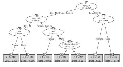
Figure 1. Parameter instability tree for identifying differences in racial FPR disparities between COMPAS and Priors. Sample sizes $n_{0}$ indicate number of observations in the terminal node for which $Y=0$. Negative values of $\Delta$ correspond to subgroups where the FPR disparity in favor of White defendants is smaller for Priors than for COMPAS.

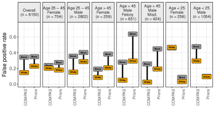
Figure 2. Differences in racial FPR disparities between COMPAS and Priors.

3. Evaluation

3.1. Recidivism risk prediction

We begin by revisiting our motivating example with ProPublica’s COMPAS data from Broward County, Florida. So far we have seen that the COMPAS score performs similarly to the priors count, Priors, in terms of overall classification metrics. To delve deeper into differences between these two recidivism prediction models, we apply our method to identify subgroups where COMPAS and Priors differ in terms of the disparity in false positive rates between Black and White defendants. The candidate splitting variables are taken to be sex, age_cat, c_charge_degree, juv_misd_count,
juv_fel_count, and juv_other_count. Figure 1 shows the resulting parameter instability tree, and Figure 2 provides a more easily interpretable representation of the findings.

Our method identifies $7$ subgroups defined in terms of sex, age_cat and c_charge_degree splits where the extent or nature of the disparity in FPR between Black and White defendants is different between the two models. For instance, as we can clearly see in rightmost panel of Figure 2, the racial FPR disparity among young men is large for COMPAS but is nearly $0$ for Priors.

We emphasize two key points. First, we observe that the Overall difference in racial FPR disparity is not reflective of differences at the subgroup level. Furthermore, we note that while the differences in FPR across the $7$ subgroups are at least in part due to differences in recidivism prevalence across the subgroups, the same argument does not explain the differences between COMPAS and Priors within the subgroups.

3.2. Sensitive attributes as inputs

Figure 3. Parameter instability tree for identifying differences in acceptance (“lending”) rates between men and women between the Small and Full models. Negative values of $\Delta$ correspond to subgroups where the acceptance rate disparity in favor of Male applicants is smaller for Full than for Small. Nodes {3, 5, 6} are later collapsed in the pruning stage as the corresponding $\Delta$’s of $0.001,0.006$ and $-0.006$, while statistically significant due to large sample sizes, are not of practical significance.

For our next example we use the Adult data set from the UCI database (Lichman, 2013) to frame a hypothetical lending problem. We fit two random forest models to the data to predict whether individuals are in the >50K income (“loan-worthy”) category. The Small model uses sex, age, workclass, education.years as inputs, while the Full model additionally uses race and marital.status, both of which are typically considered to be sensitive attributes. While we do not claim that either model is realistic, this setup does illustrate an interesting phenomenon.

We apply our method to identify subgroups where the disparity in lending rates between Male and Female applicants differs between the Small and Full model. More precisely, $\Delta$ in this example is taken to be:

$$\Delta =\left(\mathbb{P}(\hat{Y}_{\texttt{Full}}=1\mid\texttt{Male})-\mathbb{P}(\hat{Y}_{\texttt{Full}}=1\mid\texttt{Female})\right)-$$

$$\left(\mathbb{P}(\hat{Y}_{\texttt{Small}}=1\mid\texttt{Male})-\mathbb{P}(\hat{Y}_{\texttt{Small}}=1\mid\texttt{Female})\right).$$

The candidate splitting variables are taken to be education, age, marital.status and race. Figure 3 shows the resulting parameter instability tree, and Figure 4 provides a more interpretable representation of the results. Unlike in the COMPAS example, the number of terminal nodes presented in the tree differs from the number of subgroups presented in the Figure 4 summary. This is because the tree is shown prior to pruning, a final step that collapses nodes 3,5 and 6 into a single {Education <= High School} subgroup.

We observe that overall acceptance (lending) rates go up for both men and women when marital status and race is included in the model. We also find that the gender disparity in lending rates decreases—and even inverts—among Married individuals who have more than a High School education. The disparity also decreases considerably among unmarried individuals with at least a College education. However, this is largely due to the massive drop in lending rates among Men in this subgroup.

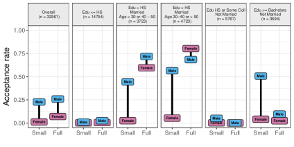
Figure 4. Differences in acceptance (“lending”) rates between men and women when marital.status and race are not included as inputs (Small) compared to when they are (Full).

4. Conclusion

This paper introduced a test-based recursive binary partitioning approach to identifying subgroups where two models differ considerably in terms of their fairness properties. Using examples in recidivism prediction and lending, we showed how this approach can be used to detect large subgroup differences in fairness that are not apparent from an overall performance comparison. The methodology can be further extended to target other kinds of disparity parameters and to use other statistical tests for parameter instability.

5. Acknowledgements

We thank the anonymous FAT/ML referees for their helpful comments on the initial version of this manuscript.

Appendix A Score test derivation

In this section we present the derivation of the likelihood and score-type test used in the partitioning scheme described in Section 2.1. This derivation is carried out for the FPR difference-in-differences parameter as defined in expression (1). Tests for other parameters of interest may be derived analogously.

Parametrization in terms of $\Delta$

For identifying partitions of covariate space on which $\Delta$ is homogeneous, it is helpful to write the distribution and its likelihood directly in terms of $\Delta$. We use the following reparameterization of the multinomial

$$\eta^{+} =p_{01}^{a_{1}}+p_{10}^{a_{1}} \delta=p_{01}^{a_{2}}+p_{10}^{a_{2}}-\eta^{+}$$

$$\eta^{-} =p_{01}^{a_{1}}-p_{10}^{a_{1}} \Delta=p_{01}^{a_{2}}-p_{10}^{a_{2}}-\eta^{-}.$$

The parameterization $(\eta^{+},\eta^{-},\delta,\Delta)$ is equivalent to
$(p_{01}^{a_{1}},p_{10}^{a_{1}},p_{01}^{a_{1}},p_{10}^{a_{1}})$, since

$$p_{01}^{a_{1}} =\left(\eta^{+}+\eta^{-}\right)/2,\quad p_{01}^{a_{2}}=\left(\eta^{+}+\delta+\eta^{-}+\Delta\right)/2$$

$$p_{10}^{a_{1}} =\left(\eta^{+}-\eta^{-}\right)/2,\quad p_{10}^{a_{2}}=\left(\eta^{+}+\delta-\eta^{-}-\Delta\right)/2.$$

Likelihood and score

The log-likelihood for this multinomial model of a sample of size $n$ with parameter $\theta=(p_{00},p_{01},p_{10},p_{11})$ is

$$\ell(\theta) =\sum_{a\in\{a_{1},a_{2}\}}\left(n_{01}^{a}\log p_{01}^{a}+n_{10}^{a}\log p_{10}^{a}+n_{\bullet}^{a}\log p_{\bullet}^{a}\right),$$

where $n_{ij}^{a}$ is the number of observations in group $A=a$ classified to $\hat{Y}_{m_{1}}=i$ and $\hat{Y}_{m_{2}}=j$. Additionally, $n_{\bullet}^{a}=n_{00}^{a}+n_{11}^{a}$, and $p_{\bullet}^{a}=1-p_{10}^{a}-p_{01}^{a}$.

For constructing the test of homogeneity, it is useful to have an expression for the score function for a single observation with respect to the parameters $(\eta^{+},\eta^{-},\delta,\Delta)$. This is given by:

$$\dot{\ell}_{i}(\theta) =\left(\frac{\partial\ell_{i}(\theta)}{\partial\eta^{+}},\frac{\partial\ell_{i}(\theta)}{\partial\eta^{-}},\frac{\partial\ell_{i}(\theta)}{\partial\delta},\frac{\partial\ell_{i}(\theta)}{\partial\Delta}\right)^{T},$$

where

$$\frac{\partial\ell_{i}(\theta)}{\partial\eta^{+}} =\frac{\mathds{1}_{01}^{a_{1}}}{2p_{01}^{a_{1}}}+\frac{\mathds{1}_{10}^{a_{1}}}{2p_{10}^{a_{1}}}+\frac{\mathds{1}_{01}^{a_{2}}}{2p_{01}^{a_{2}}}+\frac{\mathds{1}_{10}^{a_{2}}}{2p_{10}^{a_{2}}}-\frac{\mathds{1}_{\bullet}^{a_{1}}}{p_{\bullet}^{a_{1}}}-\frac{\mathds{1}_{\bullet}^{a_{2}}}{p_{\bullet}^{a_{2}}}$$

$$\frac{\partial\ell_{i}(\theta)}{\partial\eta^{-}} =\frac{\mathds{1}_{01}^{a_{1}}}{2p_{01}^{a_{1}}}-\frac{\mathds{1}_{10}^{a_{1}}}{2p_{10}^{a_{1}}}+\frac{\mathds{1}_{01}^{a_{2}}}{2p_{01}^{a_{2}}}-\frac{\mathds{1}_{10}^{a_{2}}}{2p_{10}^{a_{2}}}$$

$$\frac{\partial\ell_{i}(\theta)}{\partial\delta} =\frac{\mathds{1}_{01}^{a_{2}}}{2p_{01}^{a_{2}}}+\frac{\mathds{1}_{10}^{a_{2}}}{2p_{10}^{a_{2}}}-\frac{\mathds{1}_{\bullet}^{a_{2}}}{p_{\bullet}^{a_{2}}}$$

$$\frac{\partial\ell_{i}(\theta)}{\partial\Delta} =\frac{\mathds{1}_{01}^{a_{2}}}{2p_{01}^{a_{2}}}-\frac{\mathds{1}_{10}^{a_{2}}}{2p_{10}^{a_{2}}},$$

with $\mathds{1}_{ij}^{a}=\begin{cases}1&\text{if }\hat{Y}_{m_{1}}=i,\hat{Y}_{m_{2}}=j,\text{ and }A=a\\ 0&\text{otherwise}\end{cases}$ ,
and $\mathds{1}_{\bullet}^{a}=\mathds{1}_{00}^{a}+\mathds{1}_{11}^{a}$. In this notation, the score for the full sample is $\dot{\ell}(\theta)=\sum_{i=1}^{n}\dot{\ell}_{i}(\theta)$.

Test statistic

To test for homogeneity, we use the score-based Lagrange Multiplier test statistic of (Merkle and Zeileis, 2013). Consider a categorical splitting variable $X\in\mathbb{R}^{n}$ with levels in $\{1,\dots,K\}$. Let $\hat{\theta}$ denote the MLE of $\theta$ under the null hypothesis that $\theta$ is constant across every level of $X$. While the null is equality of the entire parameter vector $\theta$, our test statistic is constructed to have power to detect differences in $\Delta$. The test statistic is constructed as follows:

$$T =\sum_{k=1}^{K}\frac{1}{\#\{X_{i}=k\}}\left(\sum_{i:X_{i}=k}\dot{\ell}_{i}(\hat{\theta})^{T}\hat{I}(\hat{\theta})^{-1/2}e_{4}\right)^{2},$$

where $\hat{I}(\theta)=\frac{1}{n}\sum_{i=1}^{n}\dot{\ell}_{i}(\hat{\theta})\dot{\ell}_{i}(\hat{\theta})^{T}$ and $e_{4}=(0,0,0,1)^{T}$ ($\Delta$ corresponds to the fourth parameter). Under the null hypothesis that $\theta$ is constant across every level of $X$, $T$ asymptotically follows the $\chi_{K-1}^{2}$ distribution (Hjort and Koning, 2002).

References

- (1)
- Adler et al. (2016) Philip Adler, Casey Falk, Sorelle A Friedler, Gabriel Rybeck, Carlos Scheidegger, Brandon Smith, and Suresh Venkatasubramanian. 2016. Auditing black-box models by obscuring features. IEEE International Conference on Data Mining (ICDM).
- Angwin et al. (2016a) Julia Angwin, Jeff Larson, Surya Mattu, and Lauren Kirchner. 2016a. How We Analyzed the COMPAS Recidivism Algorithm. (2016). https://www.propublica.org/article/how-we-analyzed-the-compas-recidivism-algorithm
- Angwin et al. (2016b) Julia Angwin, Jeff Larson, Surya Mattu, and Lauren Kirchner. 2016b. Machine Bias: There’s Software Used Across the Country to Predict Future Criminals. And it’s Biased Against Blacks. (2016). https://www.propublica.org/article/machine-bias-risk-assessments-in-criminal-sentencing
- Athey and Imbens (2015) Susan Athey and Guido W Imbens. 2015. Machine learning methods for estimating heterogeneous causal effects. stat 1050 (2015), 5.
- Berk et al. (2017) Richard Berk, Hoda Heidari, Shahin Jabbari, Michael Kearns, and Aaron Roth. 2017. Fairness in Criminal Justice Risk Assessments: The State of the Art. arXiv preprint arXiv:1703.09207 (2017).
- Breiman et al. (1984) Leo Breiman, Jerome Friedman, Charles J Stone, and Richard A Olshen. 1984. Classification and regression trees. CRC press.
- Chouldechova (2017) Alexandra Chouldechova. 2017. Fair prediction with disparate impact: A study of bias in recidivism prediction instruments. Big data 5, 2 (2017), 153–163.
- Corbett-Davies et al. (2017) Sam Corbett-Davies, Emma Pierson, Avi Feller, Sharad Goel, and Aziz Huq. 2017. Algorithmic decision making and the cost of fairness. arXiv preprint arXiv:1701.08230 (2017).
- Datta et al. (2015) Amit Datta, Anupam Datta, Ariel D Procaccia, and Yair Zick. 2015. Influence in classification via cooperative game theory. arXiv preprint arXiv:1505.00036 (2015).
- Datta et al. (2016) Anupam Datta, Shayak Sen, and Yair Zick. 2016. Algorithmic transparency via quantitative input influence: Theory and experiments with learning systems. In Security and Privacy (SP), 2016 IEEE Symposium on. IEEE, 598–617.
- Hardt (2014) Moritz Hardt. 2014. How big data is unfair: Understanding sources of unfairness in data driven decision making. Medium. Available at: https://medium. com/@ mrtz/how-big-data-is-unfair-9aa544d739de (accessed 8 February 2015) (2014).
- Hardt et al. (2016) Moritz Hardt, Eric Price, Nati Srebro, et al. 2016. Equality of opportunity in supervised learning. In Advances in Neural Information Processing Systems. 3315–3323.
- Henelius et al. (2014) Andreas Henelius, Kai Puolamäki, Henrik Boström, Lars Asker, and Panagiotis Papapetrou. 2014. A peek into the black box: exploring classifiers by randomization. Data mining and knowledge discovery 28, 5-6 (2014), 1503–1529.
- Hjort and Koning (2002) Nils Lid Hjort and Alexander Koning. 2002. Tests for constancy of model parameters over time. Journal of Nonparametric Statistics 14, 1-2 (2002), 113–132.
- Hothorn and Zeileis (2015) Torsten Hothorn and Achim Zeileis. 2015. partykit: A Modular Toolkit for Recursive Partytioning in R. Journal of Machine Learning Research 16 (2015), 3905–3909. http://jmlr.org/papers/v16/hothorn15a.html
- Kleinberg et al. (2017) Jon Kleinberg, Sendhil Mullainathan, and Manish Raghavan. 2017. Inherent Trade-Offs in the Fair Determination of Risk Scores. In Proceedings of Innovations in Theoretical Computer Science (ITCS).
- Lichman (2013) M. Lichman. 2013. UCI Machine Learning Repository. (2013). http://archive.ics.uci.edu/ml
- Merkle and Zeileis (2013) Edgar C Merkle and Achim Zeileis. 2013. Tests of measurement invariance without subgroups: a generalization of classical methods. Psychometrika 78, 1 (2013), 59.
- Northpointe (2010) Northpointe. 2010. COMPAS Risk & Need Assessment System: Selected Questions Posed by Inquiring Agencies. (2010).
- Romei and Ruggieri (2014) Andrea Romei and Salvatore Ruggieri. 2014. A multidisciplinary survey on discrimination analysis. The Knowledge Engineering Review 29, 05 (2014), 582–638.
- Su et al. (2009) Xiaogang Su, Chih-Ling Tsai, Hansheng Wang, David M Nickerson, and Bogong Li. 2009. Subgroup analysis via recursive partitioning. Journal of Machine Learning Research 10, Feb (2009), 141–158.
- Zeileis et al. (2008) Achim Zeileis, Torsten Hothorn, and Kurt Hornik. 2008. Model-Based Recursive Partitioning. Journal of Computational and Graphical Statistics 17, 2 (2008), 492–514.
- Zhang and Neill (2016) Zhe Zhang and Daniel B Neill. 2016. Identifying Significant Predictive Bias in Classifiers. arXiv preprint arXiv:1611.08292 (2016).