How biased is your model?
Concentration Inequalities, Information and Model Bias

Abstract

We derive tight and computable bounds on the bias of statistical estimators, or more generally of quantities of interest, when evaluated on a baseline model $P$ rather than on the typically unknown true model $Q$. Our proposed method combines the scalable information inequality derived by P. Dupuis, K.Chowdhary, the authors and their collaborators together with classical concentration inequalities (such as Bennett’s and Hoeffding-Azuma inequalities). Our bounds are expressed in terms of the Kullback-Leibler divergence $R(Q\|P)$ of model $Q$ with respect to $P$ and the moment generating function for the statistical estimator under $P$. Furthermore, concentration inequalities, i.e. bounds on moment generating functions, provide tight and computationally inexpensive model bias bounds for quantities of interest. Finally, they allow us to derive rigorous confidence bands for statistical estimators that account for model bias and are valid for an arbitrary amount of data.

I Introduction

An essential ingredient of predictive modeling is the reliable calculation of specific statistics/quantities of interest of the predictive distribution. Such statistics are typically tied to the application domain, for instance moments, covariance, failure probabilities, extreme events, arrival times, average velocity, energy and so on. Predictive models can involve (a) statistical aspects or data collection, and (b) physical/mathematical mechanisms with choices in complexity/resolution, some of them potentially computationally intractable. Therefore, to improve the predictive capabilities of models we face fundamental trade-offs between model complexity, amount of available data, computational efficiency, and model bias.

The main focus of the paper is the understanding and control of model bias which often inevitably occurs in model building and which is itself a measure of reliable predictions. Our primary tool are information-theoretic Uncertainty Quantification methods. Uncertainty quantification (UQ) methods address questions related to model selection, model sensitivity, model reduction and misspecification, [1, 2, 3]. Sources of uncertainty are broadly classified in two categories: aleatoric, due to the inherent stochasticity of probabilistic models and the limited availability of data, and epistemic, stemming from the inability to accurately model all aspects of a complex system, [4, 2, 5]. Model bias is closely related to epistemic uncertainty, and probability metrics (Wasserstein, total variation) and divergences (Kullback-Leibler, Renyi, $\chi^{2}$) [6] are important tools to quantify uncertainty by comparing models. Among the divergences, the Kullback-Leibler (KL) divergence (also known as relative entropy) is widely used because of its computational tractability. Specifically, KL-based methods have been used successfully in variational inference and expectation propagation [7], model selection [8], model reduction (coarse-graining) [9, 10, 11, 12], optimal experiment design, [13], and UQ [14, 15, 16, 17].

Information-theoretic methods for model building will typically induce bias for the various statistics and the QoIs of the predictive distribution compared to the “true” model–if known–or the available data. Managing the corresponding trade-offs between a range of less biased but more computationally expensive models naturally leads to the following main question for the paper :

Can we provide performance guarantees for model bias in models built via KL-based approximate inference, model misspecification, or model selection methods?

In this paper we ultimately seek to understand how a decrease in KL-divergence–associated with an increase in modeling and/or computational effort–can guarantee a model bias tolerance; and in addition, we seek the tightest possible control of model bias. Note that bounds on the model bias of a QoI between two distributions $P$ and $Q$ can be obtained, for example, in terms of their KL or $\chi^{2}$ divergences using the classical Pinsker or Chapman-Robbins inequalities respectively, [18, 6]. Clearly a decrease in divergence will improve bounds on the model bias. However, these classical inequalities are typically non-tight and non-discriminating, in the sense that they scale poorly with the size of data sets, with the number of variables in high-dimensional models (e.g. molecular systems), or with time in the context of stochastic processes; we refer to Sections 2.2–2.3 in [19] for a complete discussion, see also the example in Remark 19.

To tackle these challenges a class of new information inequalities have been introduced by Paul Dupuis in [4] and further developed in [20, 19] by the authors and their collaborators. The resulting bounds on model bias bounds involve (a) the KL divergence $R(Q\|P)$ between a baseline model $P$ and an alternative models $Q$, and (b) the moment generating function (MGF) for the QoI under the baseline model $P$. This inequality inherits the asymmetry of $R(Q\|P)$, which in turn allows us to exchange the roles of $P$ and $Q$, depending on the context and/or availability of data from either $P$ or $Q$. Considering a neighborhood of models around the baseline $P$, defined by the KL divergence $R(Q\|P)$, can be associated with a specified error tolerance and is non-parametric in nature. The crucial mathematical ingredient behind the inequality is the Donsker-Varadhan variational principle [21, Appendix C.] for the KL divergence, also known as the Gibbs variational formula [22]. This variational representation actually implies that the new inequalities are tight, i.e. they become an equality for a suitable model $Q$ within a KL divergence neighborhood of the baseline model $P$. Furthermore, the dependence on the MGF renders the bounds scalable and discriminating for high-dimensional data sets and models, e.g. Markov Random Fields, long-time dynamics of stochastic processes and molecular models, [19] as demonstrated recently in [19]. Finally, broadly related methods in model misspecification and sensitivity analysis in financial risk measurement and queuing theory, using a robust optimization perspective, were proposed recently in [23] and [24], we also refer to references therein for other related work in operations research, finance and macroeconomics.

The primary goal of this paper is to use these new theoretical advances to develop practical tools to estimate and control model bias, and this raises new theoretical questions and implementation challenges. In particular evaluating or estimating MGFs can be very costly due to high variance of the estimators thus requiring either a large amount of data, see also Table 1, or multi-level/sequential Monte Carlo methods [25, 7, 26, 27]. In this paper we rather pursue the use of a variety of QoI-dependent concentration inequalities [28, 29, 30] to bypass the evaluation or estimation of the MGF and this leads to computable, tight bounds for model bias. Concentration inequalities are a fundamental mathematical tool in the study of rare events [31], model selection methods [32], statistical mechanics [30, Section 8.4], random matrix theory [33]. Usually concentration inequalities are used to bound tail events, i.e. to provide bounds on the probability that a random variable deviates from typical behavior. In this paper we use concentration inequalities for the purpose of uncertainty quantification, specifically to control model bias, by implementing efficiently the new information inequalities developed in [4, 20, 19], while at the same time maintaining and expanding their theoretical advantages.

The new inequalities proved in this paper— which we call concentration/information inequalities—combine concentration inequalities with the variational principles underlying the bounds and lead to model bias bounds with the following key features:

1. Easily computable bounds in terms of simple properties of the QoIs such as their mean, upper and lower bounds, suitable bounds on their variance, and so on; that is, without requiring the costly computation of MGFs.

2. Scalability for QoIs that depend on large numbers of data such as statistical estimators, or for high dimensional probabilistic models.

3. Derivation of rigorous confidence bands for statistical estimators that account for model bias and are valid for an arbitrary amount of data.

4. Applicability to families of QoIs satisfying a concentration inequality, and not to just a single QoI.

5. Tightness of the model bias bounds in the sense that the bounds are always attained within a prescribed KL-divergence and the class of QoIs in (d).

The structure of the paper is as follows. In Section II we set-up the mathematical framework for the paper and discuss the information inequalities for QoIs of [4, 20, 19]. In Section III we use concentration inequalities to derive new concentration/information inequalities on model bias that are typically straightforward to implement. In Section IV, we discuss the tightness properties of the new concentration/information bounds. Finally in Section V we study the bias of statistical estimators, noting that such QoIs will require results that scale properly with the amount of available data. We also illustrate the bounds in a variety of examples. In Section VI we consider two elementary examples with bounded or unbounded QoIs. Two examples of systems with epistemic uncertainty are discussed in Section VII; the first one deals with failure probabilities for batteries and the second with Markov Random Fields such as Ising systems.

II Tight Model Bias Bounds using KL Divergence

In coarse-graining, model reduction, model selection, or variational inference, as well as in other uncertainty quantification and approximate inference problems, a baseline model $P$ is compared to a ”true” or simply a different model $Q$. In this case the notion of risk or mean square error plays a key role in assessing the quality of the corresponding estimators. Namely, if $\hat{f}$ is an unbiased estimator of the quantity of interest $f$ for the baseline model $P$ (but not of the ”true” model $Q$) then the risk of the estimator is the mean squared error

$$\mbox{RISK}:=\mathbb{E}_{P}[(\hat{f}-\mathbb{E}_{Q}[f])^{2}]=\underbrace{{\rm Var}_{P}[\hat{f}]}_{{\rm Variance}}+\underbrace{|\mathbb{E}_{P}[f]-\mathbb{E}_{Q}[f]|^{2}}_{\rm ModelBias}\,.$$ (1)

If available computational resources can be used to control the variance of the baseline model P, then the model bias becomes the dominant source of risk thus must be carefully controlled. The main goal of this work is to understand how to transfer quantitative results on information metrics, specifically the KL divergence $R(Q\|P)$ (also known as relative entropy), to bounds on the bias for quantities of interest $f$. We formulate the corresponding mathematical problem next.

Mathematical Formulation. Let us consider a baseline model given by the probability measure $P$ on the state space $\mathcal{X}$ which we assume to be a Polish (i.e. complete separable metric) space and we consider a QoI $f$, that is a measurable function $f:\mathcal{X}\to\mathbb{R}$. We specify next a family of alternative probability distributions in terms of the Kullback-Leibler (KL) divergence (or relative entropy) $R(Q\|P)$, which is defined as

$$R(Q\|P)=\int\log\frac{dQ}{dP}dQ.$$ (2)

if $Q$ is absolutely continuous with respect to $P$ (and $+\infty$ otherwise). Note that $R(Q\|P)$ the properties of a divergence that is $R(Q\|P)\geq 0$ for all $Q$ and $R(Q\|P)=0$ if and only if $Q=P$, see e.g. [18].

We fix a positive number $\eta$ which we interpret as a level of model misspecification, quantified in terms KL divergence or, alternatively, as an error tolerance level between the baseline model $P$ and alternative models described $Q$. We then define the set of alternative probability as

$$\mathcal{Q}_{\eta}=\{Q:R(Q\|P)\leq\eta^{2}\}\,.$$ (3)

and any $Q\in\mathcal{Q}_{\eta}$ is referred to as an $\eta$-admissible model. We remark that our approach is non-parametric, i.e. it does not rely on any parametric form of the probability distributions considered. The relative entropy $R(Q\|P)$ is convex and lower-semicontinuous in $(Q,P)$. In general the set $\mathcal{Q}_{\eta}$ is infinitely dimensional, although it is compact with respect to the weak topology, [21]. The fact that the KL divergence is not symmetric in its arguments can be advantageous in some situations. For example, in variational inference, it naturally imposes a constraint on the support of the possible approximations $Q$ of a target model $P$ [7].

Our primary mathematical challenge in this work lies in quantifying the model bias in (1) if we use an $\eta$-admissible model in $Q_{\eta}$ rather than the baseline model $P$. That is we need to

$$\textrm{ Compute (or estimate) }\sup_{Q\in\mathcal{Q}_{\eta}}\{\mathbb{E}_{Q}[f]-\mathbb{E}_{P}[f]\}\quad\textrm{ and }\quad\inf_{Q\in\mathcal{Q}_{\eta}}\{\mathbb{E}_{Q}[f]-\mathbb{E}_{P}[f]\}\,.$$

Note that this approach is intrinsically goal-oriented since it includes not only a family of alternative models $Q$ but also a specific choice of QoI $f$.

Goal-oriented divergence. We now define a divergence which incorporates the QoI $f$ and hence is called goal-oriented; it was first introduced in the current form in [20] based on earlier work in [4]. Consider a QoI $f$ and the moment-generating function (MGF)

$$M_{P}(c;\tilde{f}):=E_{P}[e^{c\tilde{f}}]$$ (4)

of the centered QoI $\tilde{f}$,

$$\tilde{f}(x):=f(x)-\mathbb{E}_{P}[f].$$ (5)

In general (see [31] for details) the MGF $M_{P}(c;\tilde{f})$ is finite for $c$ in some interval $I$ and equal to $+\infty$ otherwise. Throughout this paper we will make the standing assumption that $M_{P}(c;\tilde{f})$ is finite in the interval $I=(d_{-},d_{+})$ with $d_{-}<0<d_{+}$, then under this assumption, $M_{P}(c;\tilde{f})$ is $C^{\infty}$ in $I$ and $f$ has finite moments of any order. We next define the goal-oriented (GO) divergence as

$$\Xi(Q\|P;f)=\inf_{c>0}\left\{\frac{1}{c}\log M_{P}(c;\tilde{f})+\frac{1}{c}R(Q\|P)\,\right\}.$$ (6)

for $P,Q$ with $R(Q\|p)<\infty$. Note that if $d_{+}$ is finite then the infimum can be taken on $(0,d_{+})$ and note also that if $R(Q\|P)=\infty$ then the goal oriented divergence can naturally be then set equal to $+\infty$.

In [4, 20] the following bound on the model bias was proved, along with certain mathematical properties:

Theorem 1.

Let $P$ be a probability measure and let $f$ be such that its MGF $M_{P}(c;\tilde{f})$ is finite in a neighborhood of the origin. Then for any $Q$ with $R(Q\|P)<\infty$ we have

$$-\Xi(Q\|P;-f)\leq\mathbb{E}_{Q}[f]-\mathbb{E}_{P}[f]\leq\Xi(Q\|P;f).$$ (7)

The GO divergence has the following properties

1. Divergence: $\Xi(Q\mid\mid P;f)\geq 0$ and $\Xi(Q\mid\mid P;f)=0$ if and only if either $Q=P$ or $f$ is constant $P$-a.s.

2. Linearization:

   $$\Xi(Q\mid\mid P;\pm f)=\sqrt{\mathrm{var}_{P}[f]}\sqrt{2R(Q\mid\mid P)}+O(R(Q\|P))$$

   and thus

   $$\mid E_{Q}(f)-E_{P}(f)\mid\,\leq\,\sqrt{\mathrm{var}_{P}[f]}\sqrt{2R(Q\mid\mid P)}+O(R(Q\mid\mid P)).$$

Tightness of goal-oriented divergence. Our next result complements Theorem 1 and demonstrates the tightness of the GO divergence bounds (7) for the bias of a QoI $f$; for the complete proof, we refer to Appendix (A). An equivalent tightness result for the upper bound in (13) was first shown in [4], while here we present a new formulation for a complete tightness result in Theorem 2, based on the goal-oriented divergence formulation in [20].

To state our result we introduce the exponential family $P^{c}$ given by

$$\frac{dP^{c}}{dP}\,=\,e^{cf-\log M_{P}(c;f)}\,=\,\frac{e^{cf}}{\int e^{cf}dP}\,,$$ (8)

which is well-defined for $c$ in the interval $I=(d_{-},d_{+})$ where $M_{P}(c;f)$ is finite.

Theorem 2.

Let $P$ be a probability measure and let $f$ be such the MGF $M_{P}(c;\tilde{f})$ is finite in a neighborhood of the origin. Let $\mathcal{Q}_{\eta}=\{Q:R(Q\|P)\leq\eta^{2}\}$ be the set all approximate probability $Q$ within a KL tolerance $\eta^{2}$.

1. There exists $0<\eta_{\pm}\leq\infty$ such that for any $\eta\leq\eta_{\pm}$ there are probability measures $Q^{\pm}$ such that

   $$\Xi(Q^{+}\|P;f) =\mathbb{E}_{Q^{+}}[f]-\mathbb{E}_{P}[f] =\max_{Q\in\mathcal{Q}_{\eta}}\mathbb{E}_{Q}[f]-\mathbb{E}_{P}[f],$$ (9)

   $$-\Xi(Q^{-}\|P;-f) =\mathbb{E}_{Q^{-}}[f]-\mathbb{E}_{P}[f] =\min_{Q\in\mathcal{Q}_{\eta}}\mathbb{E}_{Q}[f]-\mathbb{E}_{P}[f]$$ (10)

   The measures $Q_{\pm}$ are given by the elements $P^{c_{\pm}}$ of the exponential family (8) where $c_{\pm}$ are the unique solution of $R(P^{c_{\pm}}\|P)=\eta^{2}$.

2. If $\eta_{\pm}$ is finite then $f$ is necessarily bounded above/bounded below $P$-almost surely with upper/lower bound $f_{\pm}$. In that case, for $\eta>\eta_{\pm}$ and any $Q$ with $R(Q\|P)=\eta^{2}$ we have

   $$\Xi(Q\|P;f) =f_{+}-\mathbb{E}_{P}[f] =\sup_{Q\in\mathcal{Q}_{\eta}}\mathbb{E}_{Q}[f]-\mathbb{E}_{P}[f],$$ (11)

   $$-\Xi(Q\|P;-f) =f_{-}-\mathbb{E}_{P}[f] =\inf_{Q\in\mathcal{Q}_{\eta}}\mathbb{E}_{Q}[f]-\mathbb{E}_{P}[f]$$ (12)

The main result of the theorem provides performance guarantees in the sense that $\mathbb{E}_{Q}[f]$ belongs to the interval

$$-\Xi(Q^{-}\|P;-f)+ \mathbb{E}_{P}[f]\leq\mathbb{E}_{Q}[f]\leq \mathbb{E}_{P}[f]+\Xi(Q^{+}\|P;f)\,\quad\mbox{for all $Q\in\mathcal{Q}_{\eta}$ }$$ (13)

and the bounds are tight in $\mathcal{Q}_{\eta}$, in the sense that inequalities become equalities for $Q=Q^{\mp}$ respectively. This tightness property is crucial for our discussion because it implies that the GO divergence bounds in (7) are the best possible in the sense that they have attainable worst-case model scenarios $Q^{\pm}$ among all probability distributions $Q$ within a KL tolerance $\eta^{2}>0$, see the schematic in Figure 1.

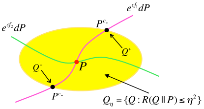
Figure 1: The schematic depiction of Theorem 2 for the QoIs $f_{1}$, $f_{2}$ with tolerance $\eta^{2}$. The solid lines depict the one-parameter tilted probability distributions $P^{c}$ corresponding to the QoIs. The theorem implies that the upper and lower bounds in the family $\mathcal{Q}_{\eta}=\{Q:R(Q\|P)\leq\eta^{2}\}$ are attained at the probability measures $Q^{\pm}=P^{c_{\pm}}$ for the QoI $f_{1}$.

Remark 3.

The tightness property (13) is a non-parametric result: the family $\mathcal{Q}_{\eta}$ of all alternative models Q cannot be parametrized in general and is only characterized by the property $R(Q\|P)\leq\eta^{2}$. In spite of this non-parametric framework, we showed in Theorem 2 that the extremal models $Q^{\pm}$ that yield the tight bounds (13) belong to the parametrized family (8), see also Figure 1.

TABLE I: For the estimation of $\mathrm{var}_{P}[Y]$, we assume that $\mathbb{E}_{P}[Y]$ is unknown and that the bias-adjusted estimator is used. For the variance of $\mathbb{E}_{P}[e^{cY}]$, a first-order approximation is used (see [34]), assuming that $\mathbb{E}_{P}[Y]$ is small.

Quantity	Variance of estimator
$E_{P}[Y]$	$\mathrm{var}_{P}[Y]/n$
$\mathrm{var}_{P}[Y]$	$2(\mathrm{var}_{P}[Y])^{2}/(n-1)$
$M_{P}(c;Y)$	$c^{2}e^{2c\mathbb{E}_{P}[Y]}\mathrm{var}_{P}[Y]/n$

The attractive properties of the GO bounds demonstrated in Theorem 1 and Theorem 2, come at a potentially significant cost since they require the knowledge or calculation of the MGF $M_{P}(c;\tilde{f})$ with respect to model $P$. If no simple formula for $M_{P}(c;\tilde{f})$ is known, this can be a data-intensive operation—compare the estimator variance of the MGF with that of other QoIs in Table I. Controlling the variance of an MGF estimator will require a large amount of data and/or the use of a multi-level Monte Carlo method, see also the discussion in Section I and Section VII.

In the next section we introduce a new class of inequalities that share the aforementioned features of the GO divergence and (7), but they can bypass the estimation of an MGF by using the concept of concentration inequalities.

III Concentration/Information Inequalities for Model Bias

To bypass the estimation or computation of the MGF in (6) we will use a QoI-dependent concentration bound for the MGF, i.e., a function $\Phi(c)$ taking values in $(0,\infty]$ such that

$$M_{P}(c;\tilde{f})\leq\Phi(c)$$ (14)

for all $c\in\mathbb{R}$. Since the moment generating function $M_{P}(c;\tilde{f})$ can take the value $+\infty$ it is natural to allow the same for $\Phi(c)$.

Bounds of the form (14), for explicitly computable functions $\Phi(c)$, are called concentration inequalities and we discuss several such examples in Section III-A and Section III-B, as well as in Section V. Although we use only the simplest concentration inequalities here, the results are indicative to what can be accomplished using such information on $f$ and $P$. In upcoming work, we will consider further applications for stochastic processes and interacting particle systems arising in Kinetic Monte Carlo and molecular dynamics models. Concentration inequalities is an important mathematical tool since they allow, via a Chernov bound, to control tail events, i.e. they provide explicit bounds on the probability that a random variable deviates from typical behavior. More specifically, such methods can address, among others, questions on rare events [31], model selection methods [32], statistical mechanics [30, Section 8.4] and random matrices [33]. Here we propose the use of concentration inequalities in tandem with the information inequalities (7) for uncertainty quantification and especially for providing model bias guarantees. In Theorem 4 we show how to construct new bounds for the model bias using a function $\Phi$ satisfying (14).

Theorem 4.

Let $P$ be a probability measure and let $f$ be a QoI such that its MGF $M_{P}(c;\tilde{f})$ is finite in a neighborhood of the origin. Let $\Phi:\mathbb{R}\to(0,\infty]$ be a function with $\Phi(0)=1$, $\Phi^{\prime}(0)=0$ and such that

$$M_{P}(c;\tilde{f})\leq\Phi(c)$$ (15)

for all $c\in\mathbb{R}$. We define the set of admissible QoIs by

$$\mathcal{F}_{P}=\{g:M_{P}(c;\tilde{g})\leq\Phi(c)\}.$$ (16)

Then, $f\in\mathcal{F}_{P}$, and for every $Q\in\mathcal{Q}_{\eta}=\{Q:R(Q\|P)\leq\eta^{2}\}$ we have

$$-U_{-}(\eta;\mathcal{F}_{P}) \leq\mathbb{E}_{Q}[g]-\mathbb{E}_{P}[g] \leq U_{+}(\eta;\mathcal{F}_{P})\,\quad\mbox{for every $g\in\mathcal{F}_{P}$}\,,$$ (17)

where

$$U_{\pm}(\eta;\mathcal{F}_{P}):=\inf_{c>0}\left\{\frac{1}{c}\log\Phi(\pm c)+\frac{1}{c}\eta^{2}\right\}.$$ (18)

Proof.

The proof follows immediately from (6) and (7), combined with the concentration inequality (15) and the definition of the admissible QoIs, $\mathcal{F}_{P}$. We discuss specific examples of inequalities of the type (15) and their corresponding admissible sets $\mathcal{F}_{P}$, in Section III-A and Section III-B below. ∎

Remark 5 (Admissible set of QoIs).

We note that the function $\Phi$ depends both on the QoI $f$ and on $P$ through (15) and therefore the set of admissible functions $\mathcal{F}_{P}$ also depends on the QoI $f$ and on $P$. However, to keep notation simple, we suppress this dependence for both $\Phi$ and $\mathcal{F}_{P}$.

Remark 6 (Computing $U_{\pm}(\eta;\mathcal{F}_{P})$).

Some concentration bounds (15) such as the sub-Gaussian and Hoeffding bounds discussed below provide explicit formulas for $U_{\pm}(\eta;\mathcal{F}_{P})$, see for instance (26) and (33). However, in general—see the sharper Bennett bounds in (28 and (30)—we have an explicit formula for $\Phi$ but no explicit closed form solution of the optimization over $c$. The elementary one-dimensional optimization in (18) can be carried out with standard solvers, e.g., Newton’s method.

Divergence structure of $U_{\pm}(\eta;\mathcal{F}_{P})$: The following properties of the bounds $U_{\pm}$ in (18) are analogous to the properties of the GO divergence (6) outlined in Theorem 1. One notable difference is that here the divergence structure defined by $U_{\pm}(\eta;\mathcal{F}_{P})$ contains information about the entire family $\mathcal{F}_{P}$ in (16) and not just a single QoI $f$ as was the case in the GO divergence (6).

Theorem 7.

Under the assumptions of Theorem 4 and, in addition, if

$$\Phi(c)=M_{\bar{P}}(c;\tilde{h})\,,$$ (19)

for some probability $\bar{P}$ and QoI $h$ and all $c\in\mathbb{R}$ then $U_{\pm}(\eta;\mathcal{F}_{P})$ satisfy:

1. Divergence Properties:

   • $U_{\pm}(\eta;\mathcal{F}_{P})\geq 0$, and

   • $U_{\pm}(\eta;\mathcal{F}_{P})=0$ if and only if $\eta=0$ or $\mathcal{F}_{P}$ is trivial, i.e. consists only of functions which are constant $P$-a.s.

2. Linearization: If $\Phi=\Phi(c)$ is twice differentiable in a neighborhood of $c=0$, then we have the asymptotics $U_{\pm}(\eta;\mathcal{F}_{P})=\sqrt{2\Phi^{\prime\prime}(0)}\eta+O(\eta^{2})$ and thus,

   $$|\mathbb{E}_{Q}[g]- \mathbb{E}_{P}[g]|\leq\sqrt{2\Phi^{\prime\prime}(0)}\eta+O(\eta^{2})\, \mbox{for all $g\in\mathcal{F}_{P}$}\quad\mbox{and all $Q\in\mathcal{Q}_{\eta}$}\,.$$ (20)

Proof.

The proof follows from Theorem 1. Indeed since, by assumption, $\Phi(c)=M_{\bar{P}}(c;\tilde{h})$ we have

$$U_{\pm}(\eta;\mathcal{F}_{P})=\Xi(Q\|\bar{P};\pm h)$$ (21)

for any probability $Q$ such that $R(Q\|\bar{P})=\eta^{2}$. Therefore, by Theorem 1, $U_{\pm}(\eta;\mathcal{F}_{P})\geq 0$ and $U_{\pm}(\eta;\mathcal{F}_{P})=0$ if and only if $\eta=0$ or $h$ is constant ${\bar{P}}$ a.s. But if $h$ is constant ${\bar{P}}$ a.s then $\Phi(c)=M_{\bar{P}}(c;\tilde{h})=1$ for all $c$ and thus the set of admissible QoIs (16) becomes:

$$\mathcal{F}_{P}=\{g:M_{P}(c;\tilde{g})\leq\Phi(c)=1\}\,.$$ (22)

However for any $g\in\mathcal{F}_{P}$, by Jensen’s inequality, $M_{P}(c;\tilde{g})\geq 1$ since $\mathbb{E}_{P}[\tilde{g}]=0$. Therefore the admissible set $\mathcal{F}_{P}$ consists only of constant functions thus $g$ is constant $P$-a.s. Finally, the linearization in Theorem 7 is proved similarly to the linearization result of the GO divergence in Theorem 1, (see the proof in Section 3 of [20]). ∎

Theorem 4 and Theorem 7 motivate the following definition, in analogy to the goal oriented (GO) divergence (6) defined for a single QoI $f$:

Definition 8 (Concentration/Information Divergence).

Given the notation and assumptions of Theorem 4 and Theorem 7, we define the concentration/information divergence between a baseline model $P$ and the family of models $\mathcal{Q}_{\eta}$, satisfying (17) for all QoIs in $\mathcal{F}_{P}$:

$$U_{\pm}(\eta;\mathcal{F}_{P}):=\inf_{c>0}\left\{\frac{1}{c}\log\Phi(\pm c)+\frac{1}{c}\eta^{2}\right\}\,,$$ (23)

where $\mathcal{Q}_{\eta}$ and $\mathcal{F}_{P}$, are defined in (3) and (16) respectively.

Remark 9 (Features of Concentration/Information Inequalities).

While the GO divergence bounds (7) are defined for a specific QoI $f$, key features of the new bounds in Theorem 4 include: (a) allow to consider whole families of admissible QoIs $\mathcal{F}_{P}$ defined in (16), and (b) they bypass the costly MGF calculations needed in the GO divergence (6). Finally, we next show that the new bounds (17) still share the advantages of the GO divergence bounds, namely: in Section IV we prove that (17) is, (c) tight in the family of models $\mathcal{Q}_{\eta}$, (3), and the family of QoIs $\mathcal{F}_{P}$, (16). in Section V we show that (17) is, (d) scalable to QoIs that depend on large numbers of data such as statistical estimators and to high dimensional probabilistic models.

We will next discuss specific examples of the bound $\Phi(c)$ in the concentration bounds (15) and Theorem 4; furthermore, we also demonstrate how we can select such concentration bounds depending on the information we have regarding the distribution $P$. We divide our presentation into two cases, namely bounded and unbounded QoIs $f$.

III-A Sub-Gaussian Bounds

For an unbounded QoI $f$ and a probability distribution $P$, we can characterize the type of concentration by bounding either the tail probabilities $P(f(X)-\mathbb{E}_{P}[f]>a)$ for all $a$ or $M_{P}(c;\tilde{f})$ for all $c$ for which the MGF is finite. In this section, we discuss the (classical) sub-Gaussian concentration bounds which are characterized by Gaussian decay of the tails. Sub-exponential bounds (see Section VI-A) and sub-Poissonian bounds could also be useful in various situations but we will not discuss them further here (see e.g. [30]).

Sub-Gaussian concentration bounds  [28] : We say that $f=f(X)$ is a sub-Gaussian random variable if there exists a $\sigma_{B}>0$ such that

$$M_{P}(c;\tilde{f})\leq\Phi(c):=\exp(c^{2}\sigma_{B}^{2}/2)\text{ for all }c\in\mathbb{R}.$$ (24)

Now given a fixed $\sigma_{B}$, we can consider the family of QoIs defined in (16),

$$\mathcal{F}_{P}:=\{g:M_{P}(c;\tilde{g})\leq\Phi(c)=\exp(c^{2}\sigma_{B}^{2}/2)\}\,,$$ (25)

i.e. we consider all random variables with MGF bounded by the MGF of a normal random variable with variance $\sigma_{B}^{2}$. Furthermore, using (18) we can write an explicit formula for $U_{\pm}(\eta;\mathcal{F}_{P})=\inf_{c>0}\{\frac{c\sigma_{B}}{2}+\frac{\eta^{2}}{c}\}$ as

$$U_{\pm}(\eta;\mathcal{F}_{P})=\sigma_{B}\sqrt{2}\eta.$$ (26)

By expanding $M_{P}(c;\tilde{f})$ around $c=0$, we can readily show that $\sigma_{B}^{2}$ is an upper bound of $\mathrm{var}_{P}[f(X)]$. Relation (26) also implies that there is no $\eta$-admissible model $Q\in\mathcal{Q}_{\eta}$ for which the QoIs under consideration lie beyond the uncertainty region given by Theorem 4:

$$-\sigma_{B}\sqrt{2}\eta\leq\mathbb{E}_{Q}[g]-\mathbb{E}_{P}[g]\leq\sigma_{B}\sqrt{2}\eta$$ (27)

for all models $Q\in\mathcal{Q}_{\eta}$ and QoIs $g\in\mathcal{F}_{P}$. In Corollary 10, we consider the special case where $P$ is a normal distribution which is compared against any models $Q$–possibly not normal–from $\mathcal{Q}_{\eta}$.

Corollary 10.

Consider the QoI $f(x)=x$ where $P=N(\mu,\sigma^{2})$. Also, let $Q$ be any distribution such that $R(Q\|P)\leq\eta^{2}$. Then, if the coefficient of variation (also known as relative standard deviation) is $c_{v}:=\sigma/|\mu|$, the relative model bias satisfies:

$$-c_{v}\sqrt{2}\eta\leq\frac{\mathbb{E}_{Q}[f]-\mathbb{E}_{P}[f]}{|\mathbb{E}_{P}[f]|}\leq c_{v}\sqrt{2}\eta\,.$$

In general, sub-Gaussianity is a strong assumption for an unbounded random variable. For example, if $P=\mathrm{Laplace}(1)$, i.e., a two-sided exponential distribution centered at zero, then $M_{P}(c;X)=1/(1-c^{2})$, $|c|<1$, which cannot be bounded by any $\exp(c^{2}\sigma_{B}^{2}/2)$ for all $c$. Finally, we note that results like the McDiarmid’s inequality, see Section V below, or the logarithmic Sobolev inequalities [29, 35], can provide values for the constant $\sigma_{B}^{2}$ for QoIs that satisfy specific properties, e.g., (43).

III-B Bennett and Hoeffding Bounds

Many quantities of interest are bounded such as failure probabilities or functions of random variables with bounded support. Bounded random variables are necessarily sub-Gaussian [28], but much sharper bounds for their MGFs, (15), can be derived and used to bound the worst-case bias through Theorem 4. In this direction, we next discuss some additional concentration bounds for bounded QoIs, that we will also showcase in examples in this work. This list is not complete by any means and other concentration inequalities can be used here, see for instance [29] for other bounds. For each case below, the family of QoIs $\mathcal{F}_{P}$ is defined in terms of the concentration bound on the MGF, (16), as in Theorem 4.

Bennett concentration bound  [31, Lemma 2.4.1]: Consider the random variable $X$ where $X\sim P$ and the QoI $f=f(X)$ such that $f(X)\leq b$, for some $0\leq b<\infty$. Setting $\mu:=\mathbb{E}_{P}[f(X)]$, $\tilde{b}:=b-\mu$, we have

$$M_{P}(c;\tilde{f})\leq\Phi(c):= \frac{\tilde{b}^{2}}{\tilde{b}^{2}+\sigma_{B}^{2}}\exp(-c\sigma_{B}^{2}/\tilde{b})+ \frac{\sigma_{B}^{2}}{\tilde{b}^{2}+\sigma_{B}^{2}}\exp(c\tilde{b}),$$ (28)

for all $c\geq 0$ and where $\sigma_{B}^{2}$ is any upper bound of $\mathrm{var}_{P}[f]$. Therefore, keeping in mind Remark 5, we define

$$\mathcal{F}_{P}= \{g:M_{P}(c;\tilde{g})\leq\Phi(c)\,\}\,, \Phi$$ where is defined in (28). (29)

Bennett-$(a,b)$ concentration bound  [31, Corollary 2.4.5]: If the QoI $f$ is such that $a\leq f(X)\leq b$, $X\sim P$, then we can set $\sigma_{B}^{2}=(\mu-a)(b-\mu)$ in the Bennett bound to obtain

$$M_{P}(c;\tilde{f})\leq\Phi(c):=\frac{\tilde{b}}{b-a}\exp(c\tilde{a})-\frac{\tilde{a}}{b-a}\exp(c\tilde{b})\text{ for all }c\in\mathbb{R}.$$ (30)

The right-hand side of (30) is the MGF of a Bernoulli-distributed random variable with values $\{a,b\}$. Note that the Bernoulli is the distribution with the most “spread” around the mean value between all bounded random variables in $[a,b]$. Similarly to (29) we have,

$$\mathcal{F}_{P}= \{g:M_{P}(c;\tilde{g})\leq\Phi(c)\,\}\,, \Phi$$ where is defined in (30). (31)

Hoeffding concentration bound [36, 31]: When the QoI $f$ is bounded as in the Bennett-$(a,b)$ case, we can further bound the Bennett-$(a,b)$ bound by a Gaussian MGF, giving rise to the (less tight) Hoeffding MGF bound,

$$M_{P}(c;\tilde{f})\leq\Phi(c):=\exp(c^{2}(b-a)^{2}/8)\text{ for all }c\in\mathbb{R}.$$ (32)

As in the sub-Gaussian case of Section III-A, we can calculate $U_{\pm}(\eta;\mathcal{F}_{P})$ explicitly:

$$U_{\pm}(\eta;\mathcal{F}_{P})=(b-a)\sqrt{2}\eta.$$ (33)

Finally the set of QoIs is

$$\mathcal{F}_{P}= \{g:M_{P}(c;\tilde{g})\leq\Phi(c)\,\}, \Phi$$ where is defined in (32). (34)

TABLE II: The different MGF bounds along with the conditions they impose on $P$ and $f$ and the quantities they depend on for their implementation if we are interested in quantifying the worst-case bias. However, bounding the worst-case $\mathbb{E}_{Q}[f]$ does not require $\mathbb{E}_{P}[f]$. Gaussian decay of the tails of the distribution of $f(X)$ implies the sub-Gaussian MGF bound (similar assumptions about the tails exist for the rest of the bounds). In terms of information requirements, the Hoeffding bound requires the least amount, but it is also the least tight. As available information/data for the bounds grow, the bounds get tighter.

Name	Conditions on $f,P$	$\Phi=\Phi(c)$ input
Hoeffding (32)	$a\leq f(X)\leq b$	$a,b$
Bennett-$(a,b)$ (30)	$a\leq f(X)\leq b$	$\mathbb{E}_{P}[f],a,b$
Bennett (28)	$f(X)\leq b$, $\mathrm{var}_{P}[f]\leq\sigma_{B}^{2}$	$\mathbb{E}_{P}[f],b,\sigma_{B}$
sub-Gaussian (24)	$M_{P}(c;\tilde{f})\leq\exp(\sigma_{B}^{2}c^{2}/2)$	$\sigma_{B}$
GO bound (6)	$M_{P}(c;\tilde{f})<\infty$	$\mathbb{E}_{P}[(f)^{k}]$ for all $k$

Remark 11 (Hierarchy of bounds).

It is straightforward to demonstrate that we can order the bounds in terms of accuracy, noting that if the QoI $f$ is bounded in $[a,b]$, then we always have the bound $\sigma_{B}^{2}\leq(\mathbb{E}_{P}[f]-a)(b-\mathbb{E}_{P}[f])$ in the Bennett bound (28). Therefore, we have the hierarchy of concentration bounds:

$$M_{P}(c;\tilde{f})\leq\text{Bennett}\leq\text{Bennett-(a,b)}\leq\text{Hoeffding}.$$ (35)

Unlike the two Bennett bounds, the Hoeffding bound is independent of the location of the mean $\mu$ within the interval $[a,b]$ and only depends on the length of the interval $b-a$. As such, it requires the least amount of information about $f$ and $P$ and is the least sharp of the bounds, see Table II and the requirements for the QoI families $\mathcal{F}_{P}$, (29), (31) and (34). On the other end, the GO divergence bound—involving $M_{P}(c;\tilde{f})$—is the tightest, as we see in (35), but also the most expensive to implement, see Table I. We also refer to a demonstration of this hierarchy in the example in Section VI-B. Overall, as available information/data on the QoI $f$ and and the baseline model $P$ grows, concentration bounds and therefore model bias bounds become tighter. Finally, we refer to Figure 2, where we demonstrate the tightness of the model bias bounds (17), (18), in terms of both $\eta^{2}=R(Q\|P)$ and $\sigma_{B}$, for the Bennett bounds (28).

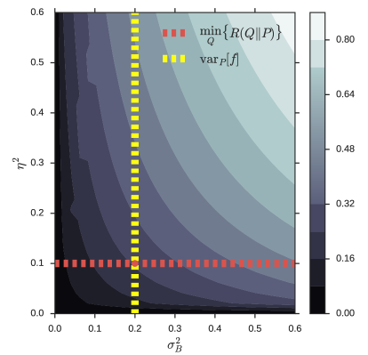
Figure 2: Level curves of the upper model bias bound (17) with the Bennett bound (28) and assuming $b=1$, $\mathrm{var}_{P}[f]\leq\sigma_{B}^{2}$. Knowing $\eta^{2}=R(Q\|P)$ for some model $Q$ and an upper bound on the variance provides model-bias guarantees (through Theorem 4). Further reduction of the model bias bound requires a corresponding—and potentially expensive—decrease in KL and/or a tighter upper-bound for $\mathrm{var}_{P}[f]$, for example, by incorporating additional data. The tightest possible guarantee afforded by the Bennett bound is gained when $\sigma_{B}^{2}=\mathrm{var}_{P}[f]$ and $\eta^{2}=\min_{Q}{R(Q\|P)}$.

Remark 12.

[How large is the class $\mathcal{F}_{P}$?] A plausible question is how rich is the set of admissible QoIs, $\mathcal{F}_{P}$ derived by the various concentration bounds on the MGF $M_{P}(c;\tilde{g})$ in (25), (29), (31) and (34). Here we address this question in the context of the Bennett bound, however the same argument also applies to the Bennett-$(a,b)$ and Hoeffding bounds, as well as to the sub-Gaussian case in Section III-A. We can get a simple first insight in this direction based on (28). Indeed, based on the conditions for this inequality to hold, we readily have that

$$\mathcal{F}_{P}\supset\{g:\;g(X)\leq b\,,\;\mathrm{var}_{P}[g]\leq\sigma_{B}^{2}\,,\;\mathbb{E}_{P}g=\mu\,\}\,.$$

We also note that enforcing the condition on the mean, $\mathbb{E}_{P}g=\mu$, is trivial and involves only a translation of the QoI $g$.

IV Tightness of the Concentration/Information Inequalities

In this section we show that, under suitable assumptions, for the concentration/information bounds derived in Section III the divergence $U_{\pm}(\eta;\mathcal{F}_{P})$ retains some of the tightness properties of the GO divergence $\Xi(Q\|P;f)$ established in Section II.

Theorem 13.

Let $P$ be a probability and $\mathcal{Q}_{\eta}=\{Q:R(Q\|P)\leq\eta^{2}\}$. Assume $\Phi(c)=M_{P}(c;\tilde{f})$ is a MGF for some QoI $f$ with respect to $P$ and let

$$\mathcal{F}_{P}=\{g:M_{P}(c;\tilde{g})\leq\Phi(c)\,\textrm{ for all }c\in\mathbb{R}\}\,.$$ (36)

Then, there exist probabilities $P^{c_{\pm}}\in\mathcal{Q}_{\eta}$ (see (8)) that satisfy $R(P^{c_{\pm}}\|P)=\eta^{2}$ and

$$U_{+}(\eta;\mathcal{F}_{P}) =\mathbb{E}_{P^{c_{+}}}[f]-\mathbb{E}_{P}[f] =\max_{Q\in\mathcal{Q}_{\eta}\,,g\in\mathcal{F}_{P}}\mathbb{E}_{Q}[g]-\mathbb{E}_{P}[g],$$ (37)

$$-U_{-}(\eta;\mathcal{F}_{P}) =\mathbb{E}_{P^{c_{-}}}[f]-\mathbb{E}_{P}[f] =\min_{Q\in\mathcal{Q}_{\eta}\,,g\in\mathcal{F}_{P}}\mathbb{E}_{Q}[g]-\mathbb{E}_{P}[g]\,,$$ (38)

i.e., the maximum and minimum for model bias is attained within the family of models $\mathcal{Q}_{\eta}$ and the family of QoIs $\mathcal{F}_{P}$, see the schematic in Figure 3. We also have the “confidence band” around the baseline model $P$,

$$-U_{-}(\eta;\mathcal{F}_{P})+\mathbb{E}_{P}[g]\leq \mathbb{E}_{Q}[g]\leq\mathbb{E}_{P}[g]+U_{+}(\eta;\mathcal{F}_{P})\, Q\in\mathcal{Q}_{\eta} g\in\mathcal{F}_{P}$$ for all ,   , (39)

with the two equalities holding if $Q=P^{c_{\mp}}$ respectively and for $g=f\in\mathcal{F}_{P}$.

Proof.

Since $f\in\mathcal{F}_{P}$, Theorem 2 implies that the probabilities $P^{c_{\pm}}$ in (8), with $c_{\pm}$ chosen such that $R(P^{c_{\pm}}\|P)=\eta^{2}$ satisfy

$$\Xi(P^{c_{\pm}}\|P;\pm f)=U_{\pm}(\eta;\mathcal{F}_{P})\,.$$ (40)

Therefore, by Theorem 4, (17), for all $Q\in\mathcal{Q}_{\eta},g\in\mathcal{F}_{P}$

$$-\Xi(P^{c_{-}}||P;-f)\leq\mathbb{E}_{Q}[g]-\mathbb{E}_{P}[g]\leq\Xi(P^{c_{+}}||P;f)\,.$$ (41)

Finally, we apply (9) and (10) of Theorem 2 and use (40) to conclude the proof. ∎

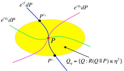
Figure 3: The schematic depiction of Theorem 13 for a family of QoIs $\mathcal{F}_{P}$ and tolerance $\eta^{2}$. The solid lines depict the one-parameter tilted probability distributions $P^{c}$ corresponding to the QoI $g_{1},g_{2},f\in\mathcal{F}_{P}$. The theorem implies that the upper and lower bounds in the family $\mathcal{Q}_{\eta}=\{Q:R(Q\|P)\leq\eta^{2}\}$ are attained at the probability measures $Q^{\pm}=P^{c_{\pm}}$.

Remark 14 (Connections to Mass Transport).

The proof of Theorem 13 is quite straightforward and we discuss here one approach to verify the crucial assumption of the Theorem, namely that

$$\Phi(c)=M_{P}(c;\tilde{f})\,\quad\mbox{for some QoI $f$\, .}$$ (42)

One natural way to ensure this is intimately related to mass transport methods, [37]. Instead of (42) we may assume the more easily checkable hypothesis that $\Phi(c)=M_{\bar{P}}(c;\tilde{h})$ for some $h$ and some model $\bar{P}$; e.g. $h(x)=x$ and $\bar{P}$ a Gaussian distribution for the Hoeffding’s bound, see also Example 16 below. To prove (42) one shows then that there exists a transport map between $P$ and $\bar{P}$, namely a map $T$ such that $\bar{P}(A)=P(T^{-1}(A))$ for any measurable set $A$ [37]. If a transport map exists we have

$$\mathbb{E}_{P}[h\circ T]=\int h(Tx)P(dx)=\int h(y)\bar{P}(dy)=\mathbb{E}_{\bar{P}}[h]\,.$$

and hence with $f=h\circ T$

$$\tilde{f}=f-\mathbb{E}_{P}[f]=h\circ T-\mathbb{E}_{\bar{P}}[h]=\tilde{h}\circ T\,.$$

This implies that

$$\Phi(c)=M_{\bar{P}}(c;\tilde{h})=\int e^{c{\tilde{h}}(y)}\bar{P}(dy)=\int e^{c{\tilde{h}}(Tx)}P(dx)=M_{P}(c;\tilde{f})\,,$$

and thus the assumption (42) holds.

To ensure the existence of such a transport map $T$ one needs some assumptions on $P$ (and $\bar{P}$). For example, if $P$ and $\bar{P}$ are non-atomic measures then a transport map always exists. If the measure $P$ has a density then $T$ can be constructed using the Knothe-Rosenblatt rearrangement or Brenier’s $L_{2}$ optimal transport map; we refer to Chapter 1 [37, 38] for more details on these maps, and several other such transport maps and relevant conditions for their existence.

Next we demonstrate how to use Theorem 13 by interpreting $\Phi(c)$ as the MGF of a suitable QoI $f$ with respect to the distribution $P$. In Example 15, we illustrate the tightness of the concentration bounds for the case of bounded random variables supported in $[-1,1]$, while the arguments can be trivially generalized to any other bounded interval.

Example 15 (Bennett-(a,b) QoIs).

Consider a distribution $P$ such that there is an event $A\subset\mathbb{R}$ such that $P(A)=1/2$; we consider the family of QoIs, $\mathcal{F}_{P}$, for which (30) is true with $a=-1$, $b=1$, $\mathbb{E}_{P}[g]=0$ for all $g\in\mathcal{F}_{P}$. The corresponding Bennett-(a,b) bound is

$$\Phi(c)=\frac{1}{2}e^{c}+\frac{1}{2}e^{-c}\,.$$

Then, if we choose $f(x):=2\cdot 1_{A}(x)-1$, where $1_{A}$ is the characteristic function of the set $A$, we have $\Phi(c)=M_{P}(c;\tilde{f})$. Therefore Theorem 13 is immediately applicable.

The next example covers the case of sub-Gaussian QoIs which contains both bounded and unbounded random variables.

Example 16 (sub-Gaussian QoIs).

Consider the probability measure $P$ on $\mathbb{R}$ which has a density. For sub-gaussian QoIs (24) we have the bound $\Phi(c)=\exp(c^{2}\sigma_{B}^{2}/2)$, however, we can rewrite the bound as

$$\Phi(c)=M_{\bar{P}}(c;\tilde{h})$$

where $h(x)=x$ and $\bar{P}=N(0,\sigma_{B}^{2})$ is a normal distribution. Since $P$ has a density, we can use the measurable isomorphism, or any other applicable map discussed in Remark 14, to construct a transport map $T$ between $P$ and $\bar{P}$. Thus, we can show the existence of a a QoI $f$ that satisfies the condition (42) and we can readily apply Theorem 13 to show the tightness of the bounds given by (26).

V Model Bias for Statistical Estimators

As discussed in Section II a key challenge is to control the risk involved in evaluating statistical estimator using the baseline model $P$ rather than the true model $Q$. In addition it is important to control the bias of QoI which are not necessarily expected values, for example the bias in the variance, i.e, $\mathrm{var}_{P}{X}-\mathrm{var}_{Q}{X}$, or other statistics such as correlation of skewness, or mean and quantiles, see [34]. Generally, given data $X_{1},\ldots,X_{n}$, we aim to control the bias of statistical estimator $\psi=\psi(X_{1},\ldots,X_{n})$, for example the sample variance (49).

To obtain useful bounds on the bias of statistical estimators $\psi$, we need to exhibit and control the dependence of the inequalities in Sections III-B and III-A on the amount of data available, i.e. the dependence on $n$. We will exhibit a large and natural class of statistical estimators for which inequalities asymptotically independent on $n$. As demonstrated in [19] the Concentration/Information inequalities of Sections II and III are the only known information equalities which scale properly with $n$.

The main tool we shall use is the key result used in the proof of the McDiarmid’s inequality, see also the Hoeffding-Azuma bound, [31]. We refer to Chapter 2 of [29] or  [39] for the proof.

Proposition 17.

Let $X_{1},\ldots,X_{n}$ be independent random variables with joint distribution $P^{n}=P_{1}\times\cdots\times P_{n}$. Let $\psi(x_{1},\ldots,x_{n})$ satisfy the Lipschitz condition

$$\sup_{x_{1},\ldots,x_{n},x_{k}^{\prime}}|\psi(x_{1},\ldots,x_{k},\ldots,x_{n})-\psi(x_{1},\ldots,x_{k}^{\prime},\ldots,x_{n})| \leq d_{k}\,.$$ (43)

for some constants $d_{k}$, $k=1,\ldots,n$. Then $\psi(X_{1},\ldots,X_{n})$ is a sub-Gaussian random variable and for all $c\in\mathbb{R}$ we have

$$M_{P^{n}}(c;\tilde{\psi}) =\mathbb{E}_{P^{n}}\left[\exp\left(c(\psi-\mathbb{E}_{P^{n}}[\psi])\right)\right] \leq\exp\left(\frac{c^{2}}{8}\sum_{k=1}^{n}d_{k}^{2}\right)\,.$$ (44)

By combining the bound in (44) with the definition of $U_{\pm}(\eta;\mathcal{F}_{P})$ in Theorem 4 for the sub-Gaussian case (24) we obtain immediately

Theorem 18.

For $X_{1},\ldots,X_{n}$ and $\psi(x_{1},\ldots,x_{n})$ as in Proposition 17 we have

$$\left|\mathbb{E}_{P^{n}}[\psi(X_{1},\ldots,X_{n})]-\mathbb{E}_{Q^{n}}[\psi(X_{1},\ldots,X_{n})]\right|= \left(\sum_{k=1}^{n}d_{k}^{2}\right)^{1/2}\sqrt{2\sum_{k=1}^{n}R(Q_{i}\|P_{i})}\,.$$ (45)

If $X_{1},\ldots,X_{n}$ are identically distributed with common distribution $P$ and if there exists a constant $C$ such that

$$d_{k}\leq\frac{C}{n}\,,\quad k=1,\ldots,n$$

then we have for any $n$

$$\left|\mathbb{E}_{P^{n}}[\psi(X_{1},\ldots,X_{n})]-\mathbb{E}_{Q^{n}}[\psi(X_{1},\ldots,X_{n})]\right|\leq C\sqrt{2R(Q\|P)}.$$ (46)

Next, we apply these results towards obtaining model bias bounds for statistical estimators.

CDF estimator: If $X$ is a real-valued with cumulative distribution function (CDF) $F_{P}(x)=P\{X\leq x\}$ then given i.i.d. data $X_{1},\ldots,X_{n}$

$${\hat{F}}_{n}(x)=\frac{1}{n}\sum_{k=1}^{n}I_{\{X_{k}\leq x\}}\,,$$ (47)

where $I_{A}$ is the indicator function of the set $A$, is an estimator for the CDF $F_{P}=F_{P}(x)$. It is easily verified that the conditions of Theorem 18 are satisfied with $C=1$. Since the bound is uniform in $x$, and ${\hat{F}}_{n}(x)$ is an unbiased estimator of $F_{P}(x)$, we obtain

$${\sup_{x}\left|F_{Q}(x)-F_{P}(x)\right|}= \sup_{x}\left|\mathbb{E}_{Q^{n}}\left[{\hat{F}}_{n}(x)\right]-\mathbb{E}_{P^{n}}\left[{\hat{F}}_{n}(x)\right]\right|\leq \sqrt{2R(Q\|P)}\,,$$ (48)

for any alternative model $Q$ to the baseline $P$. As we also note in the sample variance example below, the estimator does not need to be unbiased.

Sample variance and general statistical estimators: The McDiarmid’s inequality and the condition (43) can be used to control bias of QoIs which are not simply expected values, for example the sample variance

$$V_{n}(X_{1},\ldots,X_{n}) =\frac{1}{n-1}\sum_{i=1}^{n}\left(X_{i}-\frac{1}{n}\sum_{j=1}^{n}X_{j}\right)^{2} =\frac{1}{2n(n-1)}\sum_{i,j=1}^{n}(X_{i}-X_{j})^{2}.$$ (49)

If we assume that $|X_{i}|\leq M$ for some $M>0$ then we have

$$\sup_{\begin{subarray}{c}|x_{i}|\leq M,\\ |x_{k}^{\prime}|\leq M\end{subarray}}|V_{n}(x_{1},\ldots,x_{k},\ldots,x_{n})-V_{n}(x_{1},\ldots,x_{k}^{\prime},\ldots,x_{n})|\leq\frac{8M^{2}}{n-1}\,.$$

Then the sample variance satisfies (43) with $d_{k}=8M^{2}/(n-1)$ for all $k$. Thus, we can bound the corresponding model bias by

$$|\mathrm{var}_{P}[X]-\mathrm{var}_{Q}[X]| =|\mathbb{E}_{P^{n}}[V_{n}]-\mathbb{E}_{Q^{n}}[V_{n}]| \leq 8M^{2}\frac{n}{n-1}\sqrt{2R(Q\|P)}.$$ (50)

valid for all $n>1$. Note that if take $n\to\infty$ we obtain the variance bound

$$|\mathrm{var}_{P}[X]-\mathrm{var}_{Q}[X]|\leq 8M^{2}\sqrt{2R(Q\|P)}$$

which shows how KL-divergence $R(Q\|P)$ control the misspecification for QoIs beyond expected values. The same analysis also applies to the (biased) plug-in estimator for the variance, namely

$$\tilde{V}_{n}(X_{1},\ldots,X_{n}):=\mbox{var}_{{\hat{F}}_{n}}[X]=\frac{1}{n}\sum_{i=1}^{n}\left(X_{i}-\frac{1}{n}\sum_{j=1}^{n}X_{j}\right)^{2}\,.$$

Finally, we can easily generalize the sample variance calculation to more general QoIs and statistical estimators. The sample variance depends (up to a factor $\frac{n-1}{n}$) only on the two sample averages $\frac{1}{n}\sum_{i=1}^{n}X_{i}$ and $\frac{1}{n}\sum_{i=1}^{n}X_{i}^{2}$. It is not difficult to see that if $|X_{i}|\leq M$ and the QoI has the form

$$\psi_{n}(X_{1},\ldots,X_{n})=g\left(\frac{1}{n}\sum_{i=1}^{n}f_{1}(X_{i}),\ldots,\frac{1}{n}\sum_{i=1}^{n}f_{k}(X_{i})\right)$$ (51)

for some $f_{1},\cdots f_{k}$ (say the the first $k$ moments), and for some Lipschitz continuous function $g$, then one can apply Theorem 18 for a constant $C$ which depends on $M$, the Lipschitz constant for $g$ and $f_{1},\cdots f_{k}$. One important example of the type (51) is the sample correlation, we refer to Example 2.16 in [40].

Confidence Bands and Model Bias To further illustrate our results we construct a non-parametric confidence band for the CDF $F_{Q}(x)$. We combine the bound (48) with the Dvoretzky-Kiefer-Wolfowitz (DKW) inequality [34, 40], i.e. the bound

$$P\left\{\sup_{x}|{\hat{F}}_{n}(x)-F_{P}(x)|\geq\epsilon\right\}\leq 2e^{-2n\epsilon^{2}}\,,$$ (52)

which itself is obtained though concentration inequalities. For any $n$ and $\alpha>0$, we set $\epsilon_{n}=\sqrt{\log(2/\alpha)/2n}$ and

$$L_{n}(x;\eta)=\max\{{\hat{F}}_{n}(x)-\sqrt{2}\eta-\epsilon_{n}\,,\,0\}$$ (53)

$$U_{n}(x;\eta)=\min\{{\hat{F}}_{n}(x)+\sqrt{2}\eta+\epsilon_{n}\,,\,1\}\,.$$

Since ${\hat{F}}_{n}(x)$ is an unbiased estimator for the baseline model $P$ rather than for the (unknown) “true” model $Q$ we obtain the $\alpha$–confidence band for $F_{Q}(x)$:

$$P\left\{L_{n}(x;\eta)\leq F_{Q}(x)\leq U_{n}(x;\eta)\textrm{ for all }x\right\}\geq 1-\alpha\,,\quad\mbox{for all}\quad Q\in\mathcal{Q}_{\eta}\,.$$ (54)

Due to the fact that both our bound (48) and the DKW inequality (52) are valid for any data size $n$, the confidence band (54) does not require any asymptotic normality assumptions or a large data set $n\gg 1$.

Connections to the Vapnik-Chervonenkis inequality The DKW inequality is an effective tool for controlling deviations from the average for one dimensional distributions and their corresponding CDFs. However, the Vapnik-Chervonenkis (VC) theory [40] allows us to address the same issues in a more general setting that is applicable to higher-dimensional distributions, by considering the empirical probability distribution instead of the CDF. In particular, corresponding inequalities to (52), but for the empirical probability distribution, can be derived based on the VC theory, see for instance Theorem 2.41 and Theorem 2.43 in [40]. In turn the VC inequalities, along with our concentration information bounds (46) can allow us to obtain confidence intervals for higher dimensional distributions, similarly to (54).

Remark 19.

[Poor scalability of certain information inequalities] A notable feature of the concentration/information inequalities is that they scale independently of the number of data/random variables $n$, at least for classes of QoIs that satisfy (43), as demonstrated in Theorem 18 and the subsequent examples. Furthermore, the bias bound (46) remains discriminating even if $n\to\infty$. The same scaling features are also shared with the GO divergence bounds (7), see [19]. On the other hand, classical information inequalities scale poorly with $n$. For example, in the case of the Pinsker inequality [18, 6], let us consider the QoI (estimator) (51) for the i.i.d. random variables $X_{1},\ldots,X_{n}$,

$$\psi_{n}(X_{1},\ldots,X_{n})=\frac{1}{n}\sum_{i=1}^{n}f(X_{i})\,.$$

Then, the Pinsker inequality becomes

$$\left|\mathbb{E}_{P^{n}}[\psi(X_{1},\ldots,X_{n})]-\mathbb{E}_{Q^{n}}[\psi(X_{1},\ldots,X_{n})]\right|\leq \|f\|_{\infty}\sqrt{2R(Q^{n}\mid\mid P^{n})}=O(\sqrt{n})\,,$$ (55)

where we used that $\|\psi\|_{\infty}=\|f\|_{\infty}$, and $R(Q^{n}\mid\mid P^{n})=nR(Q\mid\mid P)$. Therefore the Pinsker bound (55) blows up as $n>>1$, in contrast to the concentration/information inequality (46) that remains discriminating and informative for any $n$. Other model bias bounds based on the Renyi or $\chi^{2}$ divergences (the latter known as the Chapman-Robbins inequality) or the Hellinger metric, also scale poorly with the size of data set and/or with the number of variables $n$; we refer to Sections 2.2–2.3 in [19] for a complete discussion.

VI Elementary examples

Prior to discussing applications involving more complex models in Section VII, here we demonstrate the concentration/information inequalities we developed earlier to two elementary examples that allow easy analytic and computational implementations.

VI-A Exponential distribution

We first consider the model bias bounds using the GO divergence in Theorem 1, contrasted to the concentration/information divergence in Theorem 4. In our first example, the baseline model $P$ is an exponential distribution. The models $Q$ can be any distributions which are absolutely continuous with respect to $P$, hence $R(Q\|P)<\infty$. Let $P$ be an exponential distribution with parameter $\lambda_{P}=1$. The QoI is $f(X)=X$. The MGF of $P$ is $M_{P}(c;X)=1/(1-c)$ and thus it is finite in $(0,1)$, while otherwise it is infinite. Next, we let $\eta$ be a model uncertainty threshold and $Q$ any distribution, not necessarily exponential or in any parametric family, such that $R(Q\|P)\leq\eta^{2}$. We note that the distribution $P$ exhibits sub-exponential behavior, namely

$$\begin{aligned} M_{P}(c;f)=1+c+\frac{c^{2}}{1-c}\leq 1+c+2c^{2}\leq\exp(c+c^{2}/(2\sigma_{B}^{2})):=\Phi(c)\,,\quad c\in(-0.5,0.5)\,,\end{aligned}$$ (56)

where $\sigma_{B}=1/2$ and the interval $(-0.5,0.5)$ is selected so that the bounds remain finite. In general, if we different information on the location of $\lambda_{P}$, e.g., from data, then we can adjust the interval that $c$ lies in accordingly. Here, the concentration/information bound (18) is then adjusted according to (56), using Theorem 4 and the general concentration bound (15). Although the MGF is known in this particular example, the use of the concentration bound (56) allows us to quantify the worst-case model bias for all QoIs $g\in\mathcal{F}_{P}$, where

$$\mathcal{F}_{P}=\{g:M_{P}(c;\tilde{g})\leq\Phi(c),\ c\in(-0.5,0.5),\ \sigma_{B}^{2}\leq 1/4\}.$$ (57)

Figure 4 is a comparison of the GO-divergence and the concentration/information bound based on (56), along with the exact model bias for the case that $Q$ is also an exponential distribution with $R(Q\|P)\leq\eta^{2}$ and $\eta\in[0,1.6]$.

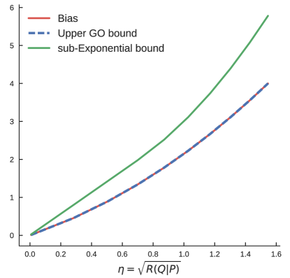
Figure 4: Comparison of model bias bounds based on the GO divergence and the concentration/information (56), with the exact model bias $1-\lambda_{Q}$, $\lambda_{Q}\in(1.01,10)$. The sub-exponential bound (56) is less sharp as the KL divergence increases, since it captures the worst-case performance over the family of QoIs $\mathcal{F}_{P}$. Although $R(Q\|P)$ is computed with $Q$ being an exponential distribution, the bounds to the model bias are valid for any $Q$ that is absolutely continuous with respect to $P$ and has $R(Q\|P)$ in the range of the figure.

Finally, we can consider other types of tail decay, and thus corresponding concentration inequalities, besides the sub-Gaussian and the sub-exponential cases discussed thus far. For example, we can also consider Poisson-type tail decay, see for instance [29, Section 3.3.5] and [41].

Remark 20.

The bias is an unbounded function of the KL divergence in this example—a consequence of the QoI $f(X)=X$ being unbounded under $P$. Therefore, any decrease in KL divergence translates to an improvement in worst-case model bias, see Figure 4; this fact is in sharp contrast with the truncated Normal example in Section VI-B, where even large improvements to larger values of the KL divergence may not help much in reducing model bias, see Figure VI-B.

VI-B Truncated Normal

In this example the distributions we consider are bounded, allowing us to deploy the hierarchy of concentration/information bounds (35) developed in Section III-B. We assume the random variable $X$ follows the truncated Normal distribution, $P=TN(0,1,-1,1)$, where $[-1,1]$ is the interval of support. Here we will bound the model bias, $\mathbb{E}_{Q}[f]-\mathbb{E}_{P}[f]$, for any $Q$ such that $R(Q\|P)=\eta^{2}$, where $\eta\in[0.01,1]$ and for any $f$ in a suitable family of QoIs, $\mathcal{F}_{P}$. Apart from these, the bounds make no other assumptions on $Q$, $f$. Figure 5 contains a comparison of the different concentration/information bounds (35) from Section III-B.

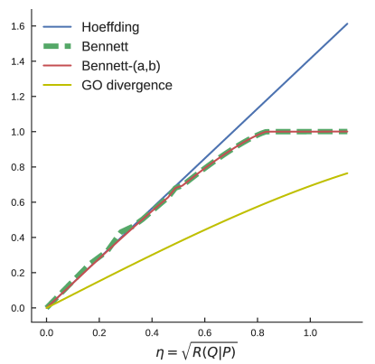
Figure 5: Comparison of the different bounds for the bias in the truncated Normal example (see Section VI-B), assuming that the observable of interest is $f(X)=X$. This plot makes no assumptions on the form of $Q$ except that $R(Q\|P)=\eta^{2}\in(0.0,4.0)$. As in Figure 4, here the concentration/information bounds capture the worst-case performance over the family of QoIs $\mathcal{F}_{P}$, hence perform worse than the GO divergence bounds which are suitable only for a single QoI, see also (35). Notice that Bennett and Bennett-$(a,b)$ track better the bound of the GO divergence for large values of the KL whereas the Hoeffding is sufficient only for small values of the KL, i.e., at the linearized regime of the GO bounds. Only the upper bounds for the bias are shown here.

As a general observation, we notice that for large values $\eta=\sqrt{R(Q\|P)}$, small perturbations of $\eta$ will not change the Bennett/GO (see Relations (6) and (28)) bounds significantly. Therefore, for some QoIs, e.g., $f(X)=X$, small improvements to large values of the KL will barely improve the worst-case bias (as captured by the bounds, see Figure 5). The existence of such QoIs is guaranteed by the sharpness of the bounds demonstrated in Section IV. Finally, we not that even for the tighter concentration/information bounds, i.e., the ones associated with the two Bennett bounds (28) and (30), there is some discrepancy with the GO divergence bound. This discrepancy is due to the fact that the GO bound is applied only for a specific QoI, while the concentration/information bounds are tight over the broad classes of QoIs defined in Section III-B, see also Remark 12.

VII Epistemic Uncertainty Quantification via Concentration/Information Inequalities

In this Section, we apply the concentration/information inequalities to control model bias between baseline and alternative models in two more complex examples. The type of model bias considered here arises in epistemic uncertainty quantification, where modelers are unsure if their baseline model included all necessary complexity or lacks sufficient data, [2, 5]. The KL divergence and in particular the GO divergence bounds provide a non-parametric framework to mathematically describe this type of epistemic uncertainties, as first shown in [4]. Here, we consider two such examples that illustrate different aspects of epistemic uncertainty, namely a data-driven model for the lifetime of lithium batteries, as well as a high-dimensional Markov Random Field model subject to various localized uncertainties such as local defects. A key aspect of our discussion in both examples is the necessity and the (ease of) implementation of concentration/information model bias bounds, see for instance Remark 21.

VII-A Epistemic Uncertainty for Failure Probabilities

Here, we apply the bounds of Theorem 4, and in particular the inequalities in Section III-B, to the life-time analysis of lithium secondary batteries. Firstly, we introduce the Weibull distribution which is widely used in for analyzing life-time data, see [42] and references therein. The probability density function of a Weibull random variable is

$$f(t)=\frac{\beta}{\xi}\left(\frac{t}{\xi}\right)^{\beta-1}e^{-(\frac{t}{\xi})^{\beta}},t>0,$$ (58)

where $\beta>0$ is called a shape parameter and $\xi>0$ is a scale parameter of the distribution [43]. The shape parameter explains the types of failure and the scale parameter explains the characteristic life cycle of devices. The cumulative distribution function $F$ can be expressed as:

$$F(T)=1-e^{-(\frac{T}{\xi})^{\beta}}\,,$$

where $T$ denotes the time of failure (or the lifetime) of the battery.

TABLE III: Failure times of test samples[42]

Specimen number	01	02	03	04	05	06	07	08	09	10	11	12
Failure time	1373	1470	1520	1427	892	814	777	637	927	688	857	866

In Table III, experimental data based on life cycle tests are obtained from [42]. By fitting the data in Table III to the parameters of the Weibull distribution, we obtain the corresponding maximum likelihood estimator (MLE) for $\xi$ and $\beta$ are $\hat{\xi}=1138$ and $\hat{\beta}=3.55$, respectively. Now, we consider this MLE Weibull distribution as the baseline model $P$, which is a data-driven approximation to the unknown true model. Next we consider the family of alternative models within a fixed tolerance $\eta^{2}$, namely the non-parametric family of models $\mathcal{Q}_{\eta}$, see (3). This family accounts for unknown features not necessarily captured in the baseline model which was arbitrarily assumed to be Weibull. Furthermore, the family $\mathcal{Q}_{\eta}$ can account for perturbations in the baseline model—constructed based on the specific dataset in Table III—due to additional data that may become available or for any errors in the data used in the MLE step.

Next, we assess the impact of model uncertainty within the family of models $\mathcal{Q}_{\eta}$ on two QoIs associated with lifetime probabilities of the batteries:

$$f_{1}(t) =1_{\{0\leq t\leq T\}}(t),t>0,$$ (59)

$$f_{2}(t;w) =\frac{1}{1+e^{w(t-T)}},t>0.$$ (60)

The function $f_{2}(t;w)$ is a commonly used smooth approximation to the indicator function $f_{1}(t)$ and is usually referred as the logistic function, see Section 39.1 of [44]). The parameter $w$, $w\geq 1$, controls the smoothness of the approximation. The QoI for the life-time probability is defined exactly as $F_{P}[T]:=E_{P}[f_{1}(t)]=P(0\leq t\leq T)$ or through the smooth approximation $\mathbb{E}_{P}[f_{2}]$.

Since the QoI $f_{1}(t)$ is bounded in $[0,1]$, we can apply the Bennett (28), Bennett-(a,b) (30) and Hoeffding bounds (32)) to obtain the uncertainty region, where $a=0$, $b=1$, $\tilde{a_{1}}=-F_{P}(T)$, $\tilde{b_{2}}=1-F_{P}(T)$ and $\sigma_{B}^{2}=Var_{P}[f_{1}(t)]$, the latter needed just in the Bennet bound. For $f_{2}$, we estimate $\mathbb{E}_{P}[f_{2}]$ by sampling from $P$, thus computing $\mu_{2}=\mathbb{E}_{P}[f_{2}]$, needed in both Bennett bounds. Then, $\tilde{a}_{2}=-\mu_{2}$ and $\tilde{b}_{2}=1-\mu_{2}$. In Figure 6 we compare the lifetime probabilities given by $f_{1}$ and $f_{2}$, where for the latter we set $w=5$. In this Figure, we also observe that the logistic function $f_{2}$ gives a good approximation of the indicator function $f_{1}$ since lifetime probabilities based on them are almost the same. Moreover, we set $\eta^{2}=0.1$ and also plot the GO divergence bounds of Theorem 1 based on $f_{1}$ and Bennett-(a,b) bounds based on $f_{2}$. We notice that the bounds almost coincide. We also consider the Bennett-(a,b) bounds based on a smaller tolerance $\eta^{2}=0.01$. As we see in the figure, we obtain a significantly narrower model bias region.

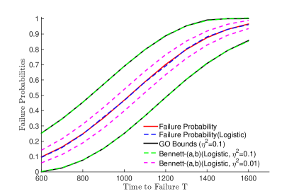
Figure 6: The blue line is the failure probability based on the logistic function $f_{2}$; The red line is the failure probability based on the indicator function $f_{1}$; The black lines are the GO bounds based on $f_{1}$ with $\eta^{2}=0.1$; The green lines are the Bennett-(a,b) bounds based on $f_{2}$ with model uncertainty $\eta^{2}=0.1$. The magenta lines are the Bennett-(a,b) bounds based on $f_{2}$ with $\eta^{2}=0.01$.

Remark 21 (Why concentration/information inequalities?).

As shown in Lemma 2.11, Equation (2.28) of [20], the $c^{*}$ that solves the optimization problem of the GO divergence bound in Equation (6) behaves like

$$c^{*}=c_{1}\eta+O(\eta^{2}),$$ (61)

for some explicit constant $c_{1}$ and $\eta^{2}=R(Q\|P)$. Due to (61) and since estimator variance for the MGF increases exponentially with $c$, a larger uncertainty threshold $\eta$ will quickly make the accurate estimation of $M_{P}(c^{*};f)$ more demanding, as is readily clear from Table I and (61). This drawback becomes especially problematic when sampling from $P$ is computationally expensive, e.g., requires MCMC sampling, $P$ is multi-modal, etc., see also the Markov Random Field example in Section VII-B, where sampling challenges can become more pronounced in higher dimensions. Even when $P$ is simple to sample, as is the case with the baseline models in [45] and here, avoiding the estimation of $M_{P}(c^{*};f)$ in the GO divergence can still save significant computational time, as Table I strongly suggests. For instance, the Bennett-(a,b) bound in (30) only requires (a) the bounds of the QoI, $a,b$, and (b) the expected value of the QoI with respect to $P$.

VII-B Uncertainty Quantification for Markov Random Fields

Here we consider the impact on QoIs of localized perturbations to statistical probability distributions of Markov Random Fields [44] such as Gibbs measures. Such distributions are inherently high-dimensional, allowing us to focus on this aspect of model bias bounds. In particular, we consider Gibbs measures for particle systems defined on a fixed finite subset $\Lambda_{N}$ of the infinite dimensional lattice $\mathbb{Z}^{d}$. Specifically we consider $\Lambda_{N}=\{x\in\mathbb{Z}^{d},|x_{i}|\leq n\}$ the square lattice with $N=(2n+1)^{d}$ lattice sites, where typically $n\gg 1$. Before we describe the model, we will specify some necessary notation: we let $S$ be the configuration space of a single particle at a lattice site $x\in\mathbb{Z}^{d}$. For example in a lattice gas model $S=\{0,1\}$, i.e. the lattice site can be empty or occupied, and in a Potts model $S=\{0,1,...,q\}$, i.e. the site is empty or occupied by particles of $q$ different species. In Ising magnetization models studied below, we have that $S=\{-1,1\}$, corresponding to down or up spins respectively. Then $S^{X}$ is the configuration space for the particles in any subset $X\subset\mathbb{Z}^{d}$; we denote by $\sigma_{X}\,=\,\{\sigma_{x}\}_{x\in X}$ an element of $S^{X}$. Next, in order to define a Gibbs measure on $\Lambda_{N}$, we first specify the Hamiltonian $H_{N}(\sigma_{\Lambda_{N}})$ of a set of particles in the region $\Lambda_{N}$. An interaction $\Phi=\{\Phi_{X}:X\subset\mathbb{Z}^{d},X\;\;\textrm{finite}\}$ associates to any finite subset $X$ a function $\Phi_{X}(\sigma_{X})$ which depends only on the particle configuration in $X$ and accounts for all particle interactions within $X$, see [22] for details. Given an interaction $\Phi$ we then define the Hamiltonian $H^{\Phi}_{N}$ (with free boundary conditions) by

$$H_{N}^{\Phi}(\sigma_{\Lambda_{N}})=\sum_{X\subset\Lambda_{N}}\Phi_{X}(\sigma_{X}),$$ (62)

and Gibbs measure $\mu_{N}^{\Phi}$ by

$$d\mu_{N}^{\Phi}(\sigma_{\Lambda_{N}})=\frac{1}{Z_{N}^{\Phi}}e^{-H_{N}(\sigma_{\Lambda_{N}})}dP_{N}(\sigma_{\Lambda_{N}}),$$ (63)

where $P_{N}$ is the counting measure on $S^{\Lambda_{N}}$ and $Z_{N}^{\Phi}=\sum_{\sigma_{\Lambda_{N}}}e^{-H_{N}(\sigma_{\Lambda_{N}})}$ is the normalization constant, also known as the partition function, [22].

Here we consider classes of perturbed models with corresponding interaction $\Psi$ that includes only local perturbations to the interaction $\Phi$, e.g. local defects encoded in the interaction potential $J$, or localized perturbations to the external field $h$ in the example of the Ising-type Hamiltonian (65). We also note that defects of finite temperature multi-scale probability distributions are a continuous source of interest in the computational materials science community, see, for instance, [46]; in fact, lattice probability distributions such as (63), constitute an important class of simplified prototype problems. In the case of localized perturbations to the interaction $\Phi$ in (62), the Hamiltonians scale as follows:

$$H_{N}^{\Psi}(\sigma_{\Lambda_{N}})=H_{N}^{\Phi}(\sigma_{\Lambda_{N}})+O(1)\,.$$

Thus the corresponding relative entropy satisfies

$$R(\mu^{\Psi}_{N}\mid\mid\mu^{\Phi}_{N}) =\log E_{\mu_{N}^{\Psi}}(e^{\Delta H})+E_{\mu_{N}^{\Psi}}(-\Delta H)$$ (64)

$$=O(1)\,,$$

uniformly in the system size $N$, where we define $\Delta H=H_{N}^{\Psi}-H_{N}^{\Phi}$. However, in most cases, we do not know the exact local perturbation as well as the perturbed Gibbs measure $\mu_{\Psi}$. Instead, based on(64) we can consider a family of perturbed models:

$$\mathcal{Q}_{\eta}=\{\mu_{\Psi}:R(\mu_{\Psi}\|\mu_{\Phi})\leq\eta^{2}\}\,.$$

This family will include any perturbation within that tolerance $\eta^{2}$, for example: defects located at different lattice sites, and of different magnitudes, as the scaling (64) demonstrates rigorously.

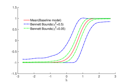
(a)

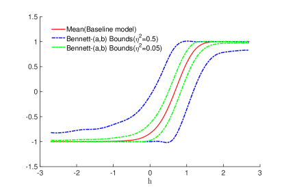
(b)

Figure 7: LABEL:sub@Fig:Ising_KL1 The red line is the mean of the QoI (66) with $m=1$ for the baseline model (65) with $J=1$ and $\beta=1$. The green and blue lines are the Bennett bounds for $\eta^{2}=0.05$ and $\eta^{2}=0.5$, respectively. LABEL:sub@Fig:Ising_KL2 The red line is the mean of the same QoI for the baseline model (65) with $J=1$ and $\beta=1$ ; The green and blue lines are the Bennett-(a,b) bounds for $\eta^{2}=0.05$ and $\eta^{2}=0.5$, respectively. In both figures the lattice size is N=100.

As a concrete example of a Hamiltonian(62), we consider $\mu_{\Phi}$ to be a one-dimensional Ising model probability distributions on the one-dimensional lattice $\Lambda_{N}$, labeled successively by $x=1,2,...,N$. To each site corresponds a spin $\sigma(x)$, with two possible values: $+1$ or $-1$. The Hamiltonian is given by

$$H^{\Phi}_{N}(\sigma_{\Lambda_{N}})=-\beta\sum_{x=1}^{N-1}J(x)\sigma(x)\sigma(x+1)-\beta h\sum_{x=1}^{N}\sigma(x).$$ (65)

Using the concentration/information inequalities developed in Section III, we can obtain model bias bounds for QoIs, such as the localized average around any lattice site $x$,

$$f(\sigma_{\Lambda_{N}})=\frac{1}{2m+1}\sum_{\{y:|y-x|\leq m\}}\sigma(y)\,,$$ (66)

for a fixed radius $m$. In the demonstration below we we pick $m=1$ for concreteness. Since the QoI $f$ (66) is bounded, $-1\leq f\leq 1$, we can use the Bennett-(a,b) bound (30). Alternatively, we can use the Bennett bound (28)), which however requires estimating in addition to $E_{\mu_{N}^{\Phi}}[f]$, the variance $Var_{\mu_{N}^{\Phi}}[f]$ by sampling from $\mu_{\Phi}$, see also Section III-B. The latter is not unreasonable given that variance computations are necessary in many applications because they ensure suitable confidence intervals for the averaged QoIs. In Figure 7, we implement both Bennett and Bennett-(a,b) bounds by considering two different KL divergence tolerances, $\eta^{2}=0.5$, $0.05$. A comparisons between Figure 7a and Figure 7b indicates that Bennett and Bennett-(a,b) bounds are fairly close for this example.

Notable computational advantages of these concentration/information inequalities over direct numerical simulation of alternative models $Q=\mu_{\Psi}$, as well as over the GO divergence bounds in Theorem 1 are the following: (1) when using Theorem 4 along with Bennett-type bounds (28) or (30), we can deploy computational resources to estimate $E_{\mu_{N}^{\Phi}}[f]$ or possibly $\mbox{Var}_{\mu_{N}^{\Phi}}[f]$—see also Table II—just for the baseline model $P=\mu_{\Phi}$, instead of simulating all alternative models $Q=\mu_{\Psi}$ models; (2) we do not need to use the full GO divergence bounds in Theorem 1, which require potentially expensive full MGF calculations, also recalling Remark 21.

VIII Conclusion

In this paper we combined the uncertainty quantification information inequality of [4, 20, 19] together with classical concentration inequalities [28] to obtain easily implementable bounds for the model bias of quantities of interest (QoIs). The bounds control the model bias in terms of the relative entropy between different models and intrinsic statistical quantities associated to the QoIs in a baseline model, e.g. mean, variance, $L^{\infty}$ bound. Our results improve substantially on classical information bounds such as the Pinsker inequality. First, our bound scales correctly with the size of the data sets/number of degrees of freedom while classical inequalities do not, see Remark 19. This scaling property is illustrated in Section V where we discuss bias bounds for general statistical estimators. In addition, we demonstrate the tightness of our bounds in Sections II and IV: given suitable families of QoIs and a family of models whose Kullback-Leibler divergence with respect to a given baseline model is less than a tolerance $\eta^{2}$, there always exists a QoI and models which saturate the upper and lower bounds. This demonstrates rigorously the precise sense our model bias bound is optimal. In forthcoming work we will apply and generalize our results to quantify model bias between different stochastic dynamics, e.g. Markov processes, in their long-time regime, bias in phase diagrams of Gibbs-Markov random fields, as well as model bias of coarse-grained models for equilibrium and non-equilibrium molecular dynamics built via variational inference methods, [9, 47].

Appendix A Proof of Theorem 2

While all the ingredients in the proof of Theorem 2 are already present in [4, 20], (see in particular [20][Theorem 2.9]), its formulation is new and we provide here a proof for completeness. Theorem 2 follows immediately from following lemma

Lemma 22.

Let $P$ be a probability measure and $f$ to be a non-constant function such that its moment generating function $M_{P}(c;\tilde{f})$ is finite in a neighborhood of $0$. Let $Q$ be such that $R(Q\|P)=M$.

1. For any $M\geq 0$ the optimization problems

   $$\Xi(Q\|P;\pm f)=\inf_{c>0}\frac{\log M_{P}(\pm c;\tilde{f})+M}{c}$$ (67)

   have unique minimizers $c^{\pm}\in[0,+\infty]$. Moreover there exists $0<M_{\pm}\leq\infty$ such that the minimizers $c^{\pm}=c^{\pm}(M)$ are finite for $M\leq M_{\pm}$ and $c^{\pm}(M)=+\infty$ if $M>M_{\pm}$.

2. If $c^{\pm}=c^{\pm}(M)$ is finite

   $$\Xi(Q\|P;\pm f)=\frac{\log M_{P}(\pm c^{\pm};\tilde{f})+M}{c^{\pm}}=\frac{d\log M_{P}}{dc}(\pm c^{\pm};\tilde{f})=\pm(\mathbb{E}_{P^{\pm c^{\pm}}}[f]-\mathbb{E}_{P}[f])\,,$$ (68)

   where $c^{\pm}(M)$ is strictly increasing in $M$ and is determined by the equation

   $$R(P^{\pm c^{\pm}}\|P)=M\,.$$ (69)

3. If $M_{\pm}<\infty$ then $f$ is necessarily $P$ almost surely bounded above/bounded below respectively with upper/lower bound $f_{\pm}$. For $M>M_{\pm}$ we have that $c^{\pm}(M)=+\infty$ and

   $$\Xi(Q\|P;\pm f)=\pm(f_{\pm}-E_{P}[f])\,.$$ (70)

Proof.

For notational ease, in the proof, let us set $H(c)=\log M_{P}(c;\tilde{f})$ and note that since $\tilde{f}$ is centered we have $H(0)=H^{\prime}(0)=0$. We have $H^{\prime}(c)=\mathbb{E}_{P^{c}}[f]-\mathbb{E}_{p}[f]$ and $H^{\prime\prime}(c)=\mathrm{Var}_{P^{c}}(f)>0$ since $f$ is not constant $P$ almost surely

If $d_{+}<\infty$ then we have $\lim_{c\to d_{+}}H(c)=\infty$ and $\lim_{c\to d_{+}}H^{\prime}(c)=\infty$. If $d_{+}=\infty$ then

$$\lim_{c\to\infty}H^{\prime}(c)=\left\{\begin{array}[]{cl}f_{+}-\mathbb{E}_{P}[f]&\textrm{ if }f\textrm{ is bounded}\\ +\infty&\textrm{ otherwise}\end{array}\right.\,.$$ (71)

Since $c^{-1}H(c)=c^{-1}\int_{0}^{c}H^{\prime}(t)dt$ and $H^{\prime}(c)$ is strictly increasing $c^{-1}H(c)$ is a strictly increasing function and we have $\lim_{c\to\infty}c^{-1}H(c)=\lim_{c\to\infty}H^{\prime}(c)$ which is finite if only if $f$ is bounded. Let us set

$$B(c;M)=\frac{\log M_{P}(c;f)+M}{c}=\frac{H(c)+M}{c}$$

and then distinguish two cases:

(a) If $d_{+}\leq\infty$ or if $d_{+}=\infty$ and $f$ is unbounded then we have $\lim_{c\to 0}B(c;M)=\lim_{c\to d_{+}}B(c;M)=+\infty$  and thus $B(c;M)$ has at least one minimum for some $0<c<d_{+}$. By calculus the minimum must be a solution of

$$0=\frac{\partial}{\partial c}B(c;M)=\frac{cH^{\prime}(c)-H(c)-M}{c^{2}}$$

that is me must have $cH^{\prime}(c)-H(c)=M$. Since $\frac{\partial}{\partial c}(cH^{\prime}(c)-H(c))=cH^{\prime\prime}(c)>0$ the function $cH^{\prime}(c)-H(c)$ is strictly increasing and thus there is a unique minimizer $c_{+}$ for $B(c;M)$.

(b) If $d_{+}=\infty$ but $f$ is bounded, since $cH^{\prime}(c)-H(c)$ is strictly increasing we have $\lim_{c\to\infty}cH^{\prime}(c)-H(c)=M_{+}$ which may or may not be finite depending on $P$. If $M\leq M_{+}$ we can proceed as in (a) to find a unique minimizer for a finite $c_{+}$, while if $M>M_{+}$, $B(c;M)$ is strictly decreasing and thus the minimizer is attained at $c_{+}=\infty$.

To conclude the proof we note that if $c_{+}<\infty$ then $c_{+}H^{\prime}(c_{+})-H(c_{+})=M$ and thus

$$B(c_{+},M)=H^{\prime}(c_{+})$$

which proves (68). On the other hand a simple computation shows that for any $c$

$$R(P^{c}\|P)=cH^{\prime}(c)-H(c)$$

and this establishes (69). Finally if $c_{+}=\infty$ the infimum is equal to $\lim_{c\to\infty}\frac{H(c)}{c}$ and this establishes (70).

∎

References

- [1] M. S. Eldred, B. M. Adams, D. M. Gay, L. P. Swiler, K. Haskell, W. J. Bohnhoff, J. P. Eddy, W. E. Hart, J. paul Watson, P. D. Hough, and T. G. Kolda, “Dakota, a multilevel parallel object-oriented framework for design optimization, parameter estimation, uncertainty quantification, and sensitivity analysis: version 5.0 user’s manual,” Tech. Rep. SAND2010-2183, Sandia National Laboratories, Tech. Rep., Dec. 2009.
- [2] R. C. Smith, Uncertainty quantification: theory, implementation, and applications. Society for Industrial and Applied Mathematics, 2013.
- [3] A. Saltelli, M. Ratto, T. Andres, F. Campolongo, J. Cariboni, D. Gatelli, M. Saisana, and S. Tarantola, Global sensitivity analysis: the primer. John Wiley & Sons, 2008.
- [4] K. Chowdhary and P. Dupuis, “Distinguishing and integrating aleatoric and epistemic variation in uncertainty quantification,” ESAIM: Mathematical Modelling and Numerical Analysis, vol. 47, no. 03, pp. 635–662, 2013.
- [5] T. J. Sullivan, Introduction to uncertainty quantification. Springer, 2015.
- [6] A. B. Tsybakov, Introduction to nonparametric estimation. Springer Science & Business Media, 2008.
- [7] C. M. Bishop, Pattern recognition and machine learning. Springer-Verlag New York, Inc., 2006.
- [8] K. P. Burnham and D. R. Anderson, Model selection and multimodel inference: a practical information-theoretic approach. Springer Science & Business Media, 2003.
- [9] A. Chaimovich and M. S. Shell, “Relative entropy as a universal metric for multiscale errors,” Physical Review E, vol. 81, no. 6, p. 060104, 2010.
- [10] M. A. Katsoulakis and P. Plecháč, “Information-theoretic tools for parametrized coarse-graining of non-equilibrium extended systems,” The Journal of chemical physics, vol. 139, no. 7, p. 074115, 2013.
- [11] J. F. Rudzinski and W. G. Noid, “Coarse-graining, entropy, forces and structures,” Journal of Chemical Physics, vol. 135, no. 21, 2011.
- [12] A. J. Majda, R. V. Abramov, and M. J. Grote, Information theory and stochastics for multiscale nonlinear systems, ser. CRM monograph series. Providence, R.I. American Mathematical Society, 2005.
- [13] A. Atkinson, A. Doney, and R. Tobias, Optimum experimental designs, with SAS. Oxford University Press, May 2007, vol. (2007). Oxford science publications. Oxford.
- [14] A. J. Majda and B. Gershgorin, “Quantifying uncertainty in climate change science through empirical information theory,” Proceedings of the National Academy of Sciences, vol. 107, no. 34, pp. 14 958–14 963, 2010.
- [15] ——, “Improving model fidelity and sensitivity for complex systems through empirical information theory,” Proceedings of the National Academy of Sciences, vol. 108, no. 25, pp. 10 044–10 049, 2011.
- [16] M. Komorowski, M. J. Costa, D. A. Rand, and M. P. Stumpf, “Sensitivity, robustness, and identifiability in stochastic chemical kinetics models,” Proceedings of the National Academy of Sciences, vol. 108, no. 21, pp. 8645–8650, 2011.
- [17] Y. Pantazis and M. A. Katsoulakis, “A relative entropy rate method for path space sensitivity analysis of stationary complex stochastic dynamics,” The Journal of chemical physics, vol. 138, no. 5, p. 054115, 2013.
- [18] T. M. Cover and J. A. Thomas, Elements of information theory. Wiley-Interscience, July 2006.
- [19] M. A. Katsoulakis, L. Rey-Bellet, and J. Wang, “Scalable information inequalities for uncertainty quantification,” Journal of Computational Physics, vol. 336, pp. 513–545, 2017.
- [20] P. Dupuis, M. A. Katsoulakis, Y. Pantazis, and P. Plechac, “Path-space information bounds for uncertainty quantification and sensitivity analysis of stochastic dynamics,” SIAM/ASA Journal on Uncertainty Quantification, vol. 4, no. 1, pp. 80–111, 2016.
- [21] P. G. Dupuis and R. S. Ellis, A weak convergence approach to the theory of large deviations, ser. Wiley series in probability and statistics. New York: Wiley, 1997.
- [22] B. Simon, The statistical mechanics of lattice gases. Princeton University Press, 2014.
- [23] P. Glasserman and X. Xu, “Robust risk measurement and model risk,” Quantitative Finance, vol. 14, no. 1, pp. 29–58, 2014.
- [24] H. Lam, “Robust sensitivity analysis for stochastic systems,” Mathematics of Operations Research, vol. 41, no. 4, pp. 1248–1275, Nov. 2016.
- [25] J. S. Liu, Monte carlo strategies in scientific computing, ser. Springer Series in Statistics. New York: Springer-Verlag, 2001.
- [26] T. Lelièvre, G. Stoltz, and M. Rousset, Free energy computations: A mathematical perspective. World Scientific, 2010.
- [27] P. Del Moral, A. Doucet, and A. Jasra, “On adaptive resampling strategies for sequential monte carlo methods,” Bernoulli, vol. 18, no. 1, pp. 252–278, Feb. 2012.
- [28] S. Boucheron, G. Lugosi, P. Massart, and M. Ledoux, Concentration inequalities : a nonasymptotic theory of independence. Oxford: Oxford University Press, 2013.
- [29] M. Raginsky, I. Sason, et al., “Concentration of measure inequalities in information theory, communications, and coding,” Foundations and Trends® in Communications and Information Theory, vol. 10, no. 1-2, pp. 1–246, 2013.
- [30] M. Ledoux, The concentration of measure phenomenon. American Mathematical Society, 2005.
- [31] A. Dembo and O. Zeitouni, “Large deviations techniques and applications,” 2010.
- [32] P. Massart, Concentration inequalities and model selection. Springer, 2007.
- [33] J. A. Tropp, “An introduction to matrix concentration inequalities,” Foundations and Trends® in Machine Learning, vol. 8, no. 1-2, pp. 1–230, 2015.
- [34] L. Wasserman, All of statistics: a concise course in statistical inference. Springer-Verlag, New York, 2004.
- [35] S. G. Bobkov and F. Götze, “Exponential integrability and transportation cost related to logarithmic sobolev inequalities,” Journal of Functional Analysis, vol. 163, no. 1, pp. 1–28, 1999.
- [36] W. Hoeffding, “Probability inequalities for sums of bounded random variables,” Journal of the American statistical association, vol. 58, no. 301, pp. 13–30, 1963.
- [37] C. Villani, Optimal transport: old and new. Springer Science & Business Media, 2008.
- [38] G. Carlier, A. Galichon, and F. Santambrogio, “From knothe’s transport to brenier’s map and a continuation method for optimal transport,” SIAM Journal on Mathematical Analysis, vol. 41, no. 6, pp. 2554–2576, 2010.
- [39] C. McDiarmid, “On the method of bounded differences,” Surveys in combinatorics, vol. 141, no. 1, pp. 148–188, 1989.
- [40] L. Wasserman, All of nonparametric statistics. Springer-Verlag New York, 2006.
- [41] S. Boucheron, G. Lugosi, P. Massart, et al., “On concentration of self-bounding functions,” Electronic Journal of Probability, vol. 14, no. 64, pp. 1884–1899, 2009.
- [42] S.-W. Eom, M.-K. Kim, I.-J. Kim, S.-I. Moon, Y.-K. Sun, and H.-S. Kim, “Life prediction and reliability assessment of lithium secondary batteries,” Journal of Power Sources, vol. 174, no. 2, pp. 954–958, 2007.
- [43] A. Papoulis and S. U. Pillai, Probability, random variables, and stochastic processes. Tata McGraw-Hill Education, 2002.
- [44] D. J. C. MacKay, Information theory, inference and learning algorithms. Cambridge University Press, 2003.
- [45] J. Li and D. Xiu, “Computation of failure probability subject to epistemic uncertainty,” SIAM Journal on Scientific Computing, vol. 34, no. 6, pp. A2946–A2964, 2012.
- [46] J. Marian, G. Venturini, B. L. Hansen, J. Knap, M. Ortiz, and G. H. Campbell, “Finite-temperature extension of the quasicontinuum method using langevin dynamics: entropy losses and analysis of errors,” Modelling and Simulation in Materials Science and Engineering, vol. 18, no. 1, p. 015003, 2010.
- [47] V. Harmandaris, E. Kalligiannaki, M. Katsoulakis, and P. Plecháč, “Path-space variational inference for non-equilibrium coarse-grained systems,” Journal of Computational Physics, vol. 314, no. C, pp. 355–383, June 2016.