Lattice polarization effects on the screened Coulomb interaction $W$ of the GW approximation

Abstract

In polar insulators where longitudinal and transverse optical phonon modes differ substantially, the electron-phonon coupling affects the energy-band structure primarily through the long-range Fröhlich contribution to the Fan term. This diagram has the same structure as the $GW$ self-energy where $W$ originates from the electron part of the screened coulomb interaction. The two can be conveniently combined by combining electron and lattice contributions to the polarizability. Both contributions are nonanalytic at the origin, and diverge as $1/q^{2}$ so that the predominant contribution comes from a small region around ${\bf q}=0$. Here we adopt a simple estimate for the Fröhlich contribution by assuming that the entire phonon part can be attributed to a small volume of ${\bf q}$ near ${\bf q}=0$. We estimate the magnitude for $\mathbf{q}{\rightarrow}0$ from a generalized Lyddane-Sachs-Teller relation, and the radius from the inverse of the polaron length scale. The gap correction is shown to agree with Fröhlich’s simple estimate $-\alpha_{P}\omega_{\mathrm{LO}}/2$ of the polaron effect with $\alpha_{P}$ the polaron couping factor.

I Introduction

The $GW$ approximationHedin (1965); Hedin and Lundqvist (1969) provides one of the most successful many-body-perturbation theoretical approaches to the electronic band structure of solids. It is based on an expansion of the self-energy in the screened Coulomb interaction $W$. In fact, the self-energy schematically is approximated as $\Sigma=iGW$ with $G$ the one-electron Green’s function. In its most recent quasiparticle self-consistent all-electron version,van Schilfgaarde et al. (2006); Kotani et al. (2007) which we label QS$GW$, it has become applicable to a wide arrange of systems. Nonetheless, it significantly overestimates the band gap in strongly ionic systems. This effect has been attributed to the neglect of ladder diagrams, which attract electron-hole pairs, enhance the screening, which reduces $W$ and the splitting between occupied and unoccupied states (see e.g. Ref. Shishkin et al., 2007). However, the lattice polarization also contributes to $W$ and enhances the screening. Previous estimates of both of these effects in literature Shishkin et al. (2007); Chen and Pasquarello (2015); Botti and Marques (2013) attribute most of the band gap overestimate by straight $GW$ to just one of these but did not consider them together.

Both electronic and polaronic terms are bosonic in origin, have the same diagrammatic structure and can be conveniently combined into a single $GW$ diagram where $W$ includes both electronic and lattice contributions to the polarizability. This fact was first used by BechstedtBechstedt et al. (2005) to modify $W$ when solving both the $GW$ band structure and the Bethe-Salpeter equation for the polarizability in strongly ionic materials. They apply the effect only in the static limit ($\omega=0$) and within the Coulomb-hole static screened exchange (COHSEX) framework. Furthermore using a model dielectric function, their correction amounts to replacing the macroscopic $\varepsilon_{\infty}$ by $\varepsilon_{0}$ in the ${\bf q}\rightarrow 0$ limit. Vidal et al. Vidal et al. (2010) estimated the renormalization of band gaps in materials with large Fröhlich coupling parameter. They adopted Bechstedt’s approach and estimate a gap reduction about 1 eV in CuAlO₂. Subsequently Botti and Marques (BM) made a refinement, taking into account the dynamics in $W$ by using a generalized Lyddane-Sachs-Teller relation.Botti and Marques (2013) However, they did not properly take into account the volume confinement of $W$ in ${\bf q}$-space.

The main physics was already laid out by Hedin Hedin and Lundqvist (1969) in the framework of many-body perturbation theory. He partitioned out the Fan term as a separate contribution to the self-energy, $iGW^{\mathrm{ph}}$; and indeed this has been the customary approach. The main effects on temperature dependent band structure and the zero-point motion corrections have been worked out in the Allen-Heine-Cardona (AHC) theory.Allen and Heine (1976); Allen and Cardona (1981, 1983) More recently both Fan and Debye-Waller contributions have been implemented in a density-functional framework. Antonius et al. (2015); Marini et al. (2015) A recent review by Giustino Giustino (2017) describes the different approaches to the electron-phonon coupling problem and points out the relations between the adiabatic AHC theory and the more general HedinHedin and Lundqvist (1969) and Baym Baym (1961) field theoretical approaches and their modern implementation. The latter rely on interpolation of the electron-phonon coupling coefficients on a fine k-point integration mesh by means of maximally localized Wannier functions.Giustino et al. (2007) This approach however becomes problematic for the long-range parts of the electron-phonon coupling in polar materials, the so-called Fröhlich part,Fröhlich (1954); Vogl (1976); Verdi and Giustino (2015); Sjakste et al. (2015) because the latter decay as $1/q$ and lead to a divergent $1/q^{2}$ contribution (and which becomes $1/q^{4}$ near band extrema if applied straightforwardly to the AHC equations). While these problems can be overcome by removing the adiabatic approximation,Giustino (2017); Poncé et al. (2015) it seems worthwhile pursuing simpler approaches to estimate the Fröhlich part of the Fan term, which dominates in compounds where $\varepsilon_{\infty}$ is small compared to $\varepsilon_{\mathrm{tot}}$.

Noting that the main problem with the Fröhlich term occurs near band edges, Nery and AllenNery and Allen (2016) developed a ${\bf k}\cdot{\bf p}$ approach for the band near the band-edge, dividing the Fan term into a non-analytic Fröhlich part and a remainder. Using the resulting simple form of the Fröhlich term, the singular integral can be done analytically and can then be combined with the numerical integration without the need for an excessively fine integration mesh. We here take their approach a step further toward simplification. As they showed, the crucial length-scale for the effect is the polaron length-scale. Therefore, we use the inverse polaron length directly as integration limit for the singular Fröhlich term. While this is a more approximate estimate than their, in principle, exact approach, which subtracts the singularity from the numerical integration and replaces it by the analytical result for a simple model, we use directly the simple model and estimate the size of the region in ${\bf q}$-space where it is applicable as the inverse polaron length.

The BM approach is another option worth revisiting. This is the main goal of our paper. We identify the problem in BM’s treatment of the ${\bf q}\rightarrow 0$ limit. Again, our solution is to base this on the polaron-length scale. We show that the BM approach, as is, depends crucially on the size of the integration mesh and the gap correction decreases proportional to $1/N_{\rm mesh}$ and would thus go to zero at convergence. Instead, we assume that the correction applies in a finite ${\bf q}$-region of size the inverse polaron length. The advantage compared to a full evaluation of the Fröhlich contribution to the Fan terms is that the computational effort is vastly simpler; moreover the phonon contribution to the entire band structure is obtained in a single calculation.

We apply both approaches to a set of strongly ionic materials, MgO, NaCl, LiF, LiCl and show that the modified BM approach leads to results in good agreement with the above simplified Nery-Allen polaronic estimate. We also consider zincblende GaN for a direct comparison to Nery and Allen’s more complete approach, although the effect here is an order of magnitude smaller. Admittedly, our approach does not address the full electron-phonon coupling renormalization of the band gap, only the Fröhlich part. However, for strongly ionic materials, this is arguably the largest contribution. The other electron-phonon contributions to the zero-point motion correction are large only in systems with only light atoms. Finally, we consider the relative importance of this effect to the effects of missing electron-hole interactions based on literature data. The conclusion is that the latter are in fact a more important correction to the band-gap reduction.

II Theory

As is well known,Maradudin et al. (1971); Gonze and Lee (1997) optical phonon modes can strongly modify the screening in polar compounds. This is nicely encapsulated by the generalized Lyddane-Sachs-Teller (LST) relation in the $\mathbf{q}{\rightarrow}0$ limit

$$\frac{\varepsilon_{tot}^{\alpha}(\mathbf{q}\rightarrow 0,\omega)}{\varepsilon_{el}^{\alpha}(\mathbf{q}\rightarrow 0,\omega)}=\prod_{m}\frac{\left(\omega^{\alpha}_{\mathrm{LO};m}\right)^{2}-\omega^{2}}{\left(\omega_{\mathrm{TO};m}\right)^{2}-(\omega+i0^{+})^{2}}.$$ (1)

The product runs over all optical modes $m$ which are infrared active and have a longitudinal-transverse splitting ($\omega_{\mathrm{LO};m}>\omega_{\mathrm{TO};m}$) and belong to the irreducible representation corresponding to the polarization direction $\alpha$. The superscript $\alpha$ indicates the direction along which $\mathbf{q}{\rightarrow}0$ approaches zero and the LO modes depend on this direction. We next examine, how this affects the screened Coulomb interaction $W$ in the $GW$ theory.

In practical calculations, $W(\mathbf{q},\mathbf{r},\mathbf{r}^{\prime},\omega)$ is represented by an expansion in a basis set. In our all-electron implementationKotani et al. (2007) this consists of a mixed product basis with Bloch sums of products of of partial waves inside augmentation spheres and plane waves in the interstitial. Thus $W$ becomes a matrix $W_{\mu\nu}(\mathbf{q},\omega)$. More commonly plane waves are used for these bosonic degrees of freedom, in which case $\mu$ becomes ${\bf G}$. As noted already the effect is dominant in the $\mathbf{q}{\rightarrow}0$ limit. Treatment of $W_{\mu\nu}(\mathbf{q}{\rightarrow}0,\omega)$ requires special care because of the divergence of the Coulomb interaction $v(\mathbf{q})=4\pi e^{2}/q^{2}$. (There is a similar divergence for Fröhlich contribution.) It is however integrable, because what is needed for the self-energy is a convolution integral over both energy and wave vector,

$$\Sigma^{c}_{nm}({\bf k},\omega) = \frac{i}{2\pi}\int d\omega^{\prime}\sum_{\mathbf{q}}^{\mathrm{BZ}}\sum_{n^{\prime}}^{\mathrm{all}}G_{nn^{\prime}}({\bf k}-\mathbf{q},\omega-\omega^{\prime})$$ (2)

$$\sum_{\mu\nu}W^{c}_{\mu\nu}(\mathbf{q},\omega^{\prime})e^{-i\delta\omega^{\prime}}$$

$$\langle\psi_{{\bf k}n}|\psi_{{\bf k}-\mathbf{q}n^{\prime}}E_{\mu}^{\mathbf{q}}\rangle\langle E_{\nu}^{\mathbf{q}}\psi_{{\bf k}-\mathbf{q}n^{\prime}}|\psi_{{\bf k}m}\rangle.$$

The sum over $\mathbf{q}$ becomes an integral and the contribution from the region near $\mathbf{q}=0$ over a small sphere multiplies the divergence by $q^{2}dq$. Here the Green’s function $G_{nn^{\prime}}({\bf k}-\mathbf{q},\omega-\omega^{\prime})=[\omega-\omega^{\prime}-\epsilon_{{\bf k}-\mathbf{q}}\pm i\delta]^{-1}\delta_{nn^{\prime}}$, is a diagonal matrix in the basis of one-electron states,$\psi_{{\bf k}n}$; the screened Coulomb interaction is expanded in an auxiliary mixed product basis set $E_{\mu}$ which diagonalizes the bare Coulomb matrix,Friedrich et al. (2010) and conversion factors from one basis to the other are included. The superscript $c$ refers to taking the correlation part $W^{c}=W-v$.

The approach dealing with this integrable divergence has been described by Freysoldt et al. Freysoldt et al. (2007) in the context of a plane wave basis set expansion of the bare and screened Coulomb interaction and by Friedrich et al. Friedrich et al. (2009, 2010) in terms of a mixed product basis set expansion. The method consists in replacing the integral over the BZ by an exactly integrable function with the same type of divergence. The difference between the two is then a smooth function for which the integral can be replaced by a discrete sum. The approach originally was introduced by Massida et al. Massidda et al. (1993) in Hartree-Fock calculations because, in fact, the same problem already affects the bare exchange. In the context of $GW$ theory, it requires a knowledge of the screened Coulomb interaction near $\mathbf{q}=0$ and this can either be obtained by an analytical ${\bf k}\cdot{\bf p}$ approachFriedrich et al. (2010) or by using the offset-$\Gamma$ method. The actual approach used in the QSGW programeca is described in Kotani et al. Kotani (2014) and provides an improved version of the offset-$\Gamma$ method used in Ref. Kotani et al., 2007. To obtain the behavior $W(\mathbf{q})$ near $\mathbf{q}=0$, one needs the macroscopic inverse dielectric constant, which is $1/\varepsilon^{-1}_{00}(\mathbf{q}{\rightarrow}0,\omega)$. It is calculated by a block matrix inversion separating out the divergent term from the known behavior of the polarizability matrix as function of $\mathbf{q}$. Here the subscripts $00$ of the dielectric function matrix refer to the reciprocal lattice vector ${\bf G}=0$ in a plane wave basis set, or equivalently the first mixed-product basis set function in the basis set that diagonalizes the bare Coulomb interaction.Friedrich et al. (2010) Both of these in fact correspond to the average over the unit cell. The inverse of this quantity is then expanded in spherical harmonics and only the $L=00$ spherical average is required for the integral of the “head” of $\varepsilon^{-1}_{00}$. This is if we neglect some higher order corrections, discussed by Betzinger et al. Betzinger et al. (2010)

For a simple estimate of the phonon contribution, we use the fact that (1) the Fröhlich contribution to $W$ originates predominately from the divergent, small-$q$ region,Nery and Allen (2016) and (2) we handle this region using the usual formulation of the $GW$ self-energy calculation through a special treatment of the integrable divergence of $W$ in the neighborhood of $\mathbf{q}=0$ only. Eq. (2) is integrated numerically on a discrete $\mathbf{q}$ mesh, and the “central” cell term is treated specially to handle the divergence. Our approach simply modifies the central cell dielectric function $\varepsilon^{-1}_{00}(\mathbf{q}{=}0)$ using the appropriate Lyddane-Sachs-Teller factor. The fact that its limit is non-analytic, i.e. depends on the direction of $\mathbf{q}$ means that it is a second rank tensor with non-zero components dictated by symmetry. For example for an orthorhombic crystal, it will have only diagonal components but the $xx$, $yy$ and $zz$ diagonal elements are all different. In general in the anisotropic offset-$\Gamma$ methodKotani (2014) it is expanded in invariant tensors corresponding to the symmetry of the cell and requires at most six $\mathbf{q}$ points close to $\mathbf{q}=0$ where the macroscopic dielectric constant must be evaluated and for which we need to know the corresponding LO-TO splittings.

In a full approach to the electron-phonon coupling, one can arbitrarily cut out some small region near the singularity, subtract the standard mesh integration technique result for that region and replace it by the properly integrated singularity. This is the approach followed by Nery and Allen.Nery and Allen (2016) Here we focus exclusively on the Fröhlich term, and thus we cannot rely on a cancellation of the two treatments to the self-energy integral. We thus need an accurate estimate of the range of the polaron effect. In the treatment of the $\mathbf{q}{\rightarrow}0$ limit for the purely electronic screening, the relative weight of the specially treated $\Gamma$-cell depends on the size of the $\mathbf{q}$-point mesh. The finer the mesh, the less the weight of the $\Gamma$-cell. The electron-phonon contribution should not depend on the mesh spacing, but since we lump the entire contribution into the central cell and omit contributions from other microcells, the Fröhlich contribution to $W_{00}(\mathbf{q}{=}0,\omega)$ should be rescaled as described below.

We may decouple the convergence in $\mathbf{q}$-space of the electronic polarizability from that of the phonon contribution as follows. We define the LST factor $f_{\rm LST}$ to be the factor that corrects $W$, so that the additive correction is $\Delta W=(f_{\rm LST}-1)W$. At $\mathbf{q}{=0}$, $f_{\rm LST}$ is the inverse of the factor in Eq. (1). Now, according to the above discussion, we want to correct the $\mathbf{q}{=0}$ value of $W$ but this represents an effective volume in q-space. So, we need to estimate separately the size of this ${\bf q}$-space region over which the effect of the lattice polarization is to be taken into account. Let’s call this $q_{\mathrm{LP}}$ and the corresponding volume $\Omega_{\mathrm{LP}}=q_{\mathrm{LP}}^{3}$. When we calculate the convolution integral $\Delta\Sigma({\bf k})=\sum_{\mathbf{q}}G({\bf k}-\mathbf{q})\Delta W(\mathbf{q})$ as a discrete sum, we assume only the $\mathbf{q}{=0}$ microcell of volume $\Omega_{GW}=\Omega_{BZ}/N_{\mathrm{mesh}}$ contributes, so $\Delta\Sigma({\bf k})=iG({\bf k})\Delta W(0)$. If the GW mesh is coarser than $q_{LP}$, than we might overestimate the effect. On the other hand if it is finer, than the phonon correction should be extended to GW-mesh points beyond ${\bf k}=0$. Instead, we may simply rescale $\Delta{W}(0)$ to $W(0)\Omega_{\mathrm{LP}}/\Omega_{GW}$. This means that for the pure electronic screening part, the usual compensation between the discrete sum (non-divergent part) and the special treatment of the $\Gamma$-cell is still valid. But for the added $\Delta\Sigma=i(f_{\rm LST}-1)G({\bf k})W(0)\Omega_{\mathrm{LP}}/\Omega_{GW}$ we use a fixed volume of $\mathbf{q}$-space corresponding to $q_{\mathrm{LP}}$

The essential problem to obtain meaningful results within this approach is thus to pick $q_{\mathrm{LP}}$. We note that it cannot be obtained from considerations of the phonons or of the dependence of $\varepsilon_{tot}({\bf q})/\varepsilon_{el}({\bf q})$ alone because the latter lack information on the electron-phonon coupling to the bands, which must involve the effective masses of the bands. Following Nery and Allen’s idea,Nery and Allen (2016) the relevant length scale here is the polaron length $a_{P}=\sqrt{\hbar/2\omega_{LO}m_{*}}$, where $\omega_{LO}$ is the longitudinal phonon for which we consider the electron-phonon contribution and $m_{*}$ is the band effective mass. This means there is actually a different polaron length for electrons and holes, which we denote $a_{Pe}$ and $a_{Ph}$. Using an electron (hole) effective mass of 0.35 (1.26) for MgO as an example, we obtain polaron length scales of 20.84 and 10.96 $a_{0}$ ($a_{0}$ is the Bohr radius). We use $(2m_{hh}+m_{lh})/3$ along the [100] direction for the holes. We use this type of average because the heavy hole band is doubly degenerate. The average $a_{P}=(a_{Pe}+a_{Ph})/2$ defines an inverse length scale of 0.06 $a_{0}^{-1}$ which for MgO is about 1/12 of the BZ. Typically, for a two atom unit cell system like MgO, a $8\times 8\times 8$ mesh already gives both the $GW$ and phonons very well converged. We also found that the gap correction in the BM approach varies as $1/N_{\mathrm{mesh}}$. We can thus extrapolate to the appropriate $q=1/a_{P}$ or use the approach for decoupling from the mesh-size described in the previous paragraph. The precise way of averaging the effective masses here is not crucial because we only are trying to estimate the polaron length and the results are not very sensitive to this estimate.

The approach described here is similar to that of Botti and Marques Botti and Marques (2013), except that they did not take into account the range of the Fröhlich interaction. In their formulation the effect would have vanished in the limit of small microcell size.

They also appeared to confuse the relevant length scale: they said “It is easy to understand that the coupling of phonon waves and electromagnetic waves is effective only for ${\bf q}\rightarrow 0$, since the speed of sound is negligible if compared with the speed of light.” This is true but rather irrelevant to the problem considered here. In fact, the coupling of electromagnetic waves to phonon waves, i.e. polariton formation, following PickPick (1970), occurs only when $q=|{\bf q}|\gg\omega_{0}/c$ with $\omega_{0}$ a typical phonon frequency and $c$ the speed of light. Decoupling occurs for $q\ll\omega_{0}/c$. This is about $q=10^{-4}$ of the Brillouin zone (BZ). In other words, this theory provides a cut-off above rather than below which the effect comes into play. However, we are not concerned with the retardation effects of polariton formation here, we are interested in the applicability of the LST relation and the polaronic effect on the band gap.

We may also directly estimate the Fröhlich singularity integral. Following Nery and Allen, Nery and Allen (2016) the singular contribution near the band edge to the zero-point motion self-energy is given by

$$\Delta E_{n{\bf k}}=-\alpha_{P}\hbar\omega_{\mathrm{LO}}\tan^{-1}{(q_{F}a_{\mathrm{LO}})}\frac{2}{\pi},$$ (3)

where

$$\alpha_{P}=\frac{e^{2}}{2a_{P}}\frac{1}{\hbar\omega_{\mathrm{LO}}}\left[\frac{1}{\varepsilon_{\infty}}-\frac{1}{\varepsilon_{0}}\right],$$ (4)

is the dimensionless polaron coupling constant. The question now is what to use as integration cut-off $q_{F}$ for the upper limit of the Fröhlich singularity integral. Clearly an overestimte will be obtained if we use $q_{F}=q_{BZ}=2\pi/a$ because the expression is supposed to be valid only over the region where the band dispersion is parabolic. It is even customary to let $q_{F}\rightarrow\infty$, in which case we obtain $-\alpha\hbar\omega_{\mathrm{LO}}$ as upper limit.Fröhlich (1954) In Nery and Allen’s approach this choice is not crucial because they look at where this explicit approach becomes equivalent to the standard integration approach of the other electron-phonon coupling terms besides the long-range Fröhlich one. This occurs at about 1/6 of the BZ in their case of GaN. A better estimate would be $q_{F}=1/a_{P}$; then the inverse tangent factor is simply $\pi/4$ and Eq. (3) simplifies to

$$\Delta E_{n{\bf k}} = -\alpha_{P}\omega_{\mathrm{LO}}/2,$$ (5)

$$= \frac{e^{2}}{4a_{P}}\left(\varepsilon_{\infty}^{-1}-\varepsilon_{0}^{-1}\right),$$

where if $n$ corresponds to the conduction band minimum (CBM), we use $a_{Pe}$ and if $n$ corresponds to the valence band maximum (VBM), we would use $a_{Ph}$ as polaron lengths. So, this is simply half the difference in Coulomb interaction at the polaron length calculated with purely electronic screening and electronic plus lattice screening. This differs from the upper limit by only a factor of 2, so the estimation of $q_{F}$ is not very crucial if our goal is to obtain the right order of magnitude. For the example of GaN used by Nery and Allen, we find this already gives an excellent approximation to their full calculation. We will show that it also agrees well with the modified BM approach described above, in which $q_{LP}$ is also set to $1/a_{P}$.

We emphasize again, that if one applies the electron-phonon coupling fully at all q-points then one can subtract out the region of the singularity from the mesh sum and add it back in integrated analytically. However, in the BM approach we focus entirely on the singular contribution, and thus we are limited by how reliably we estimate the size of the singularity. This is true both if one thinks of it as a Fröhlich coupling strength dipole singularity or as the $1/q^{2}$ singularity in the $W$ screened Coulomb potential. In fact, both are essentially the same. and both give a correction proportional to $\varepsilon_{\infty}^{-1}-\varepsilon_{0}^{-1}$ and inversely proportional to $a_{P}$.

As far as the frequency dependence is concerned, it is clear from Eq.(1) that for $\omega>\omega_{\mathrm{LO}}$ the factor quickly goes to 1. Therefore in the integral over frequency, it is sufficient to apply the effect only at $\omega=0$ as long as the first non-zero $\omega$-mesh point is already well above $\omega_{\mathrm{LO}}$. If one wishes to apply the effect including its frequency dependence, then one needs to use a sufficiently fine integration mesh near the $\omega_{\mathrm{TO}}$ and $\omega_{\mathrm{LO}}$ phonons to carry out the integrals over these poles correctly. We have done both and find that reliable results can be obtained using a coarse mesh, and scaling $W(\mathbf{q}{=0},\omega{=}0)$ only. This is further discussed in the Appendix A. Since a very fine frequency mesh is required if the pole is properly summed over, this greatly simplifies the computational effort.

III Computational details

All calculations before are carried out using the QS$GW$ approach in the LMTO basis set implementation,Kotani et al. (2007) which can be found on-line at Ref.eca, . The relevant phonons are taken from experiment or can be calculated using the ABINIT program.Gonze et al. (0211)

The experimental lattice constants were used, MgO (4.21 ÅFei (1999)), NaCl (5.64 ÅGray (1963)), LiCl (5.14 ÅEwald and Hermann (1931)), LiF (4.02 ÅEwald and Hermann (1931)). In the QS$GW$ calculation, for MgO we used semicore Mg $2p$ and high lying $3s$ states as local orbital for the completeness of basis set. For NaCl, we also used semicore $2p$ as local orbitals.

IV Results and discussion

Table 1: Parameters used to calculate the polaron length and polaron coupling strength in various materials and the polaron shifts of the band edges and gap. Effective masses in units of free electron mass, $m_{h}=(2m_{hh}+m_{lh})/3$. Phonon frequency $\omega_{\mathrm{LO}}$ in cm^-1, polaron lengths $a_{Pe}$ and $a_{Ph}$ in Bohr units $a_{0}$. Polaron coupling constants $\alpha_{Pe}$ and $\alpha_{Ph}$ for electrons and holes are dimensionless. Energy shifts in meV.

	MgO	NaCl	LiF	LiCl	GaN
$m_{e}$	0.35	0.35	0.61	0.40	0.18
$m_{hh}[100]$	1.70	2.10	2.83	1.06	1.70
$m_{lh}[100]$	0.40	0.55	1.10	0.56	0.50
$m_{h}$	1.26	1.58	2.25	0.89	1.30
$\omega_{\mathrm{LO}}$ (cm-1)	722	265	656	382	730
$a_{Pe}$ ($a_{0}$)	20.8	34.4	16.6	26.8	28.9
$a_{Ph}$ ($a_{0}$)	11.0	16.2	8.6	17.9	10.7
$a_{P}$ ($a_{0}$)	15.9	25.3	12.6	22.4	19.8
$\varepsilon_{\infty}$	3.0	2.3	1.95	2.8	5.6
$\varepsilon_{0}$	9.8	5.9	9.0	11.2	9.9
$\alpha_{Pe}$	1.7	3.2	4.1	2.9	0.4
$\alpha_{Ph}$	3.2	6.9	7.8	4.4	1.1
$\Delta E_{CBM}$ (meV)	75	53	165	69	18
$\Delta E_{VBM}$ (meV)	144	113	317	103	49
$\Delta E_{g}$ (meV)	219	166	483	172	67

In Table 1 we show the polaron lengths and coupling strengths for electrons and holes as well as the parameters entering them. The effective masses are obtained from fitting the QS$GW$ calculations before adding the lattice polarization correction. The dielectric constants are taken from experiment but could also be calculated in DFT using for example the ABINIT program or using the electronic band structure within QS$GW$ for $\varepsilon_{\infty}$ and calculating $\varepsilon_{0}$ using the LST factor. Finally it shows the estimated band edge and gap shifts using Eq. 5. We note that for GaN, this amounts to 67 meV, close to Nery and Allen’s own estimate of 50 meV, especially when considering that we expect an errorbar of order 10 meV in view of the various approximations made. We may note that typically the shift is larger for the VBM because of the shorter polaron length because of the larger hole mass. For NaCl, we may compare our result with Fröhlich’s own estimate of the conduction band shift.Fröhlich (1954) He used an effective mass $m_{e}=1$ and obtained 0.18 eV. Using $m_{e}=1$ we would obtain 0.09 eV differing by a factor $2$ because in Fröhlich’s estimate the upper limit of the singularity integral is replaced by $\infty$.

Table 2: Band gaps in LDA, QSGW, QSGW+LPC in the BM approach with different k-meshes and extrapolated to $q_{LP}=1/a_{P}$, as well as the zero-point motion (ZPM) correction to the gap. All values in eV. The % change in QSGW-LDA gap correction due to LPC is also given.

	MgO	NaCl	LiF	LiCl	GaN
LDA	4.65	5.01	9.43	6.32	1.76
QSGW	8.69	9.44	16.19	10.19	3.54
QSGW+LPC-BM-6	7.99	8.80	14.87	9.52	3.31
QSGW+LPC-BM-8	8.20	8.99	15.32	9.71	3.50
QSGW+LPC	8.43	9.26	15.64	9.98	3.50
ZPM-Fröhlich	-0.26	-0.18	-0.55	-0.21	-0.04
ZPM-polaron	-0.22	-0.17	-0.48	-0.17	-0.07
QSGW-LDA	4.04	4.43	6.76	3.87	1.78
% change LPC	-6	-4	-8	-5	-2
QSGW-BM	8.94	9.52	15.81	10.28
QSGW+LPC-BMa	7.71	8.37	13.69	9.05
ZPM-BMa	-1.23	-1.15	-2.12	-1.23
Expt. gap	7.8	8.5	14.2	9.4	3.5$\pm 0.1$

Next we compare the above polaron estimates of the band edge shift with the results of the modified BM approach, in which we use the average polaron length $a_{P}$ to set the $q_{LP}=1/a_{P}$. In this table, we show the LDA gaps, the QS$GW$ gaps and the QS$GW$ gaps with the BM-type lattice polarization correction using $N_{\mathrm{mesh}}=6$ or 8. We note that the QS$GW$ results are well converged already with a $6\times 6\times 6$ mesh, which differ from the $8\times 8\times 8$ mesh by only 0.1 eV. However, the LPC correction is then effectively applied only to a smaller region and has less weight. Therefore the corresponding QS$GW$+LPC-BM-8 gap is less reduced than the QS$GW$+LPC-BM-6 one. We then extrapolate from the $q_{\mathrm{LP}}=(2\pi/a)(1/N_{\mathrm{mesh}})$ to $q_{\mathrm{LP}}=1/a_{P}$ assuming linear dependence. This is the result labeled QSGW+LPC. Finally, the zero-point-motion correction, due to the lattice-polarization correction, labeled ZPM-Fröhlich in Table 2 is the difference between the QSGW+LPC and QSGW gaps and should be compared with the polaron effect given in Table 1. Rounding the values of $\Delta E_{g}$ of Table 1 to 0.01 eV, a more realistic estimate of the uncertainty, we obtain the results in the row labeled ZPM-polaron. We can see that the two estimates agree with each other to within a few 0.01 eV. Comparing with the gaps and gap reduction values given by Botti and Marques in the next few rows, we see that their calculation significantly overestimated the effect. This is primarily because they used a $6\times 6\times 6$ mesh but there are also differences in the QS$GW$ results themselves which result from their use of a pseudopotential approximation and a plane wave basis set compared to our all-electron and LMTO basis set. Finally, we also give the experimental gaps.

We note that our QS$GW$ gap for MgO is lower than that of BM (8.94 eV) or Shishkin et al. Shishkin et al. (2007) (9.16 eV) or Chen and PasquarelloChen and Pasquarello (2015) (9.29 eV). We note that if we use a less converged basis set (leaving out the higher energy 3s local orbitals on O for example, we also find a higher gap). We therefore caution that comparisons of the lattice-polarization effect in $GW$ between different methods should also keep in mind that differences between all-electron and pseudopotential methods as well as various convergence issues may play a role.

Our adjusted gaps still overestimate the experimental gaps. This indicates that the electron-hole effects on the gap reduction may be more important than the lattice polarization correction. For MgO, the results of Shishkin et al. Shishkin et al. (2007) and Chen et al. Chen and Pasquarello (2015) indicate effects of the order of 20% of the QSGW-LDA gap correction. The under-screening in the QS$GW$ due to the lack of electron-hole interactions or random phase approximation, was noted before and for most semiconductors amounts to about 20%. This has led to a commonly used correction factor of $0.8\Sigma$.Chantis et al. (2006); Deguchi et al. (2016). A universal factor of 0.8 can be approximately justified because $\varepsilon_{\infty}$ is uniformly underestimated by a factor of 0.8 in a wide range of semiconductors. The results of Chen et al. Chen and Pasquarello (2015) and ShishkinShishkin et al. (2007) MgO and NaCl, and LiCl further support this. Our results indicate a further reduction of this gap correction by the lattice polarization by about 5%. The percentage reduction of the QSGW-LDA gap correction due to the lattice polarization effect is given in Table 2 and varies from 2-8 %. Taken together this would reduce the QSGW-LDA gap correction by 25 %. The zero-point motion correction of the gap in MgO was previously estimated to be 0.15-0.19 eV for MgO.Antonius et al. (2015) but it is not clear whether this properly includes the long-range Fröhlich contribution. Assuming it is not and adding the present Fröhlich lattice polarization correction, the total zero-point-motion correction would then amount to 0.4 eV.

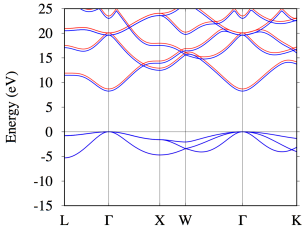
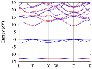
Figure 1: (Color-online) Band structure of MgO (top) and NaCl (bottom), the red color for QS$GW$ and blue for QS$GW$+LPC with $N_{\mathrm{mesh}}=8$.

One advantage of our modified BM approach is that in principle it not only corrects the gap but the entire band structure. Plotting the full band structures, as shown in Fig. 1 for two examples MgO and NaCl, and for $N_{\mathrm{mesh}}=8$ we find that the effect amounts pretty much to a constant shift of the conduction band once the valence bands are aligned. Using the fixed mesh size may still somewhat overestimate the effect on the gap as seen from Table 2 but nonetheless allows us to estimate how it affects the rest of the band structure. This constant shift is by no means guaranteed because it is not clear immediately whether the same polaron length-scale estimates of the required integration region of the ${\bf q}\rightarrow 0$ singularity, $q_{\mathrm{LP}}$ applies also to other bands. Our calculation assumes that this can be taken the same for all bands. At present we are not aware of experimental evidence to test this result of a constant shift.

V Conclusions

In this paper, we revisited the approach proposed by Botti and MarquesBotti and Marques (2013) to estimate the lattice polarization effect on $W$ in the $GW$ method and hence on the band structure in ionic materials. As pointed out by GiustinoGiustino (2017) the BM approach is equivalent to the Fröhlich contribution to the Fan self-energy, which has thus far only received limited attention in spite of the large amount of work on electron-phonon coupling renormalization of the band gaps of materials. This is primarily due to the technical difficulties in calculating it, which require a very fine ${\bf k}$-space integration mesh.

We develop here a simplied approach which takes advantage of the fact that the Frölich interaction is dominant in a small region around $\mathbf{q}$=0. The effective volume of $\mathbf{q}$ is fixed by the polaron length scale $a_{P}=\sqrt{\hbar/2\omega_{\mathrm{LO}}m_{*}}$. With this length scale for the Frölich interaction, and the LST relations at $W(\mathbf{q}{=0})$, we can construct a simple description that modifies $W$ directly, which can be used both in $GW$ calculations and for higher order diagrams involving $W$, e.g. incorporation of ladder diagrams via the Bethe-Salpeter equation Rohlfing and Louie (2000), with minimal cost.

We compared our results of the BM method with a simple estimate based on directly integrating the Fröhlich electron-phonon coupling singularity near the band gap and find that the latter can also be estimated simply by setting the cut-off of the singularity integral to the inverse polaron length. We note that the present method allows us to estimate the gap correction to at best a few 0.01 eV only because of the remaining uncertainty in the polaron length $a_{P}$. For a more refined treatment to meV prevision a full electron-phonon calculation of the band shifts will be required and would allow adjusting $a_{P}$ to fit it.

Appendix A Discussion of the $\omega\rightarrow 0$ limit.

Here, we address the issue of whether we need the $\omega$-dependence of the LST factor. As far as the frequency dependence is concerned, we can in principle include the frequency dependent LST factor as given in Eq.(1) in the main text. However, in evaluating $\Sigma$ we then need to make sure the extra pole due to the phonon is properly integrated over. The method for calculating the energy integral in Eq.(2) in the main text is described in detail in Sec. II.F of Ref. Kotani et al., 2007. It is done with a contour integral mostly along the imaginary axis but including pole contributions from the energy bands along the real axis. The inclusion of the lattice polarization effect through the LST factor introduces poles in $W(\omega)$ close to $\omega=0$ in the energy range of the phonons, more precisely at the $\omega_{LO}$ frequencies. We thus need to ensure that these do not lead to spurious effects and are adequately integrated over. The behavior of $W$ near $\omega\rightarrow 0$ along the imaginary axis is already taken care of specially in Ref. Kotani et al., 2007. The band structure poles, however lead to a contribution $W^{c}(\omega-\epsilon_{{\bf k}-{\bf q}n})$. These are tabulated on an $\omega$-mesh along the real axis for later interpolation of $\Sigma(\omega)$ to the values required. For example, in the QS$GW$, method one needs $\left[\Sigma_{nm}(\epsilon_{{\bf k}m})+\Sigma_{nm}(\epsilon_{{\bf k}n})\right]/2$. Thus this mesh must be chosen fine enough so that adequate interpolation is possible if $\omega-\epsilon_{{\bf k}n}\approx 0$ for some energy band. Unphysical values would result if this energy band is close to the pole. One may avoid a divergence by adding a small imaginary part to the $\omega$ and using a fine mesh in the region of the phonons. However, for a reasonable $\omega$-mesh spacing for the electronic part of $W^{c}$, all except the first point $\omega=0$ are usually well above the phonon frequencies where the LST factor goes to 1. Thus, we may also only correct the $\omega=0$ mesh-point where the correction factor is simply $\prod_{m}\omega_{LOm}^{2}/\omega_{TOm}^{2}$. We have tested both approaches and found that they give the same result for the final band gap. In fact, intuitively, one does not expect the detailed behavior near each phonon to have a specific effect. Such an effect would occur whenever some energy band difference $\epsilon_{{\bf k}n}-\epsilon_{{\bf k}-{\bf q}n^{\prime}}$ is close to an LO phonon energy and leads to an almost divergent contribution $W^{c}(\omega_{LO})$. This means that the $\omega$-dependence of the LST factor, which is one of the distinguishing features of BM compared to the previous work of BechstedtBechstedt et al. (2005) who only applied the correction to the static part of $\Sigma$ is not as important as one might guess at first sight and Bechstedt’s approach is adequate, especially in view of the other approximations we are already making and the overal goal to keep this approach as simple as possible.

Table 3: The band gap (in eV) in MgO as function of $d\omega$ (in Rydberg), the mesh size along the real frequency axis used in the calculation of $\Sigma$.

$d\omega$	0.0002	0.0005	0.004	0.01	0.02
$E_{g}$	8.06	7.95	7.89	8.12	8.08

We compare results with different real $d\omega$ mesh sizes for MgO. This $d\omega$ corresponds to the mesh spacing used in the interpolation of $\Sigma(\omega)$ as mentioned earlier. From Table 3, we see that for $d\omega=0.0002$ Ry the band gap is 8.06 eV which is very close to the value when we use a large mesh spacing $d\omega=0.02$ Ry. So, either we pick the mesh so fine the phonon region is integrated and interpolated over correctly, or we pick it big enough so we just skip over it and effectively only include the correction at the first $\omega=0$ point. However, for intermediate values of $d\omega$, the gap seems to vary in a somewhat uncontrolled way. This results from the difficulty of interpolating the rapidly varying LST correction factor of Eq.(1) in the region near the phonon frequency. It is clear that the latter goes through an asymptote at $\omega_{T}$, or its inverse goes through an asymptote at $\omega_{L}$. Thus the value can rapidly change from positive to negative and unreliable results are obtained if the integration mesh samples just a few random points on this curve. In fact, note that the $\omega_{T}\approx 0.003$ Ryd. in this case of MgO and hence $d\omega=0.0002$ is sufficiently fine compared to $\omega_{T}$ and $d\omega=0.02$ is sufficiently large to just skip over the whole range, while $d\omega\approx 0.004$ is troublesome. We conclude from this that correcting only the $\omega=0$ value is more efficient and sufficiently accurate. Similar results are obtained for NaCl. However in that case, the relevant phonon frequencies are significantly smaller and hence an even finer and ultimately, unpractical mesh would be required.

References

- Hedin (1965) L. Hedin, Phys. Rev. 139, A796 (1965).
- Hedin and Lundqvist (1969) L. Hedin and S. Lundqvist, in Solid State Physics, Advanced in Research and Applications, Vol. 23, edited by F. Seitz, D. Turnbull, and H. Ehrenreich (Academic Press, New York, 1969) pp. 1–181.
- van Schilfgaarde et al. (2006) M. van Schilfgaarde, T. Kotani, and S. Faleev, Phys. Rev. Lett. 96, 226402 (2006).
- Kotani et al. (2007) T. Kotani, M. van Schilfgaarde, and S. V. Faleev, Phys.Rev. B 76, 165106 (2007).
- Shishkin et al. (2007) M. Shishkin, M. Marsman, and G. Kresse, Phys. Rev. Lett. 99, 246403 (2007).
- Chen and Pasquarello (2015) W. Chen and A. Pasquarello, Phys. Rev. B 92, 041115 (2015).
- Botti and Marques (2013) S. Botti and M. A. L. Marques, Phys. Rev. Lett. 110, 226404 (2013).
- Bechstedt et al. (2005) F. Bechstedt, K. Seino, P. H. Hahn, and W. G. Schmidt, Phys. Rev. B 72, 245114 (2005).
- Vidal et al. (2010) J. Vidal, F. Trani, F. Bruneval, M. A. L. Marques, and S. Botti, Phys. Rev. Lett. 104, 136401 (2010).
- Allen and Heine (1976) P. B. Allen and V. Heine, Journal of Physics C: Solid State Physics 9, 2305 (1976).
- Allen and Cardona (1981) P. B. Allen and M. Cardona, Phys. Rev. B 23, 1495 (1981).
- Allen and Cardona (1983) P. B. Allen and M. Cardona, Phys. Rev. B 27, 4760 (1983).
- Antonius et al. (2015) G. Antonius, S. Poncé, E. Lantagne-Hurtubise, G. Auclair, X. Gonze, and M. Côté, Phys. Rev. B 92, 085137 (2015).
- Marini et al. (2015) A. Marini, S. Poncé, and X. Gonze, Phys. Rev. B 91, 224310 (2015).
- Giustino (2017) F. Giustino, Rev. Mod. Phys. 89, 015003 (2017).
- Baym (1961) G. Baym, Annals of Physics 14, 1 (1961).
- Giustino et al. (2007) F. Giustino, M. L. Cohen, and S. G. Louie, Phys. Rev. B 76, 165108 (2007).
- Fröhlich (1954) H. Fröhlich, Advances in Physics 3, 325 (1954), http://dx.doi.org/10.1080/00018735400101213 .
- Vogl (1976) P. Vogl, Phys. Rev. B 13, 694 (1976).
- Verdi and Giustino (2015) C. Verdi and F. Giustino, Phys. Rev. Lett. 115, 176401 (2015).
- Sjakste et al. (2015) J. Sjakste, N. Vast, M. Calandra, and F. Mauri, Phys. Rev. B 92, 054307 (2015).
- Poncé et al. (2015) S. Poncé, Y. Gillet, J. L. Janssen, A. Marini, M. Verstraete, and X. Gonze, The Journal of Chemical Physics 143, 102813 (2015), http://dx.doi.org/10.1063/1.4927081 .
- Nery and Allen (2016) J. P. Nery and P. B. Allen, Phys. Rev. B 94, 115135 (2016).
- Maradudin et al. (1971) A. A. Maradudin, E. W. Montroll, G. H. Weiss, and I. P. Ipatova, Theory of Lattice Dynamics in the Harmonic Approximation, second edition ed. (Academic Press, New Yor, 1971).
- Gonze and Lee (1997) X. Gonze and C. Lee, Phys. Rev. B 55, 10355 (1997).
- Friedrich et al. (2010) C. Friedrich, S. Blügel, and A. Schindlmayr, Phys. Rev. B 81, 125102 (2010).
- Freysoldt et al. (2007) C. Freysoldt, P. Eggert, P. Rinke, A. Schindlmayr, R. W. Godby, and M. Scheffler, Computer Physics Communications 176, 1–13 (2007).
- Friedrich et al. (2009) C. Friedrich, A. Schindlmayr, and S. Blügel, Computer Physics Communications 180, 347 (2009).
- Massidda et al. (1993) S. Massidda, M. Posternak, and A. Baldereschi, Phys. Rev. B 48, 5058 (1993).
- (30) Our implementation was adapted from the original ecalj package, now at (https://github.com/tkotani/ecalj/). It is available at http://www.questaal.org, together with the one-body part.
- Kotani (2014) T. Kotani, Journal of the Physical Society of Japan 83, 094711 (2014), http://dx.doi.org/10.7566/JPSJ.83.094711 .
- Betzinger et al. (2010) M. Betzinger, C. Friedrich, and S. Blügel, Phys. Rev. B 81, 195117 (2010).
- Pick (1970) R. M. Pick, Adv. Phys. 19, 269 (1970).
- Gonze et al. (0211) X. Gonze, J. M. Beuken, R. Caracas, F. Detraux, M. Fuchs, G. M. Rignanese, M. Sindic, L.and Verstraete, G. Zerah, and F. Jollet, Computational Materials Science 25,3, 478 (2002/11).
- Fei (1999) Y. Fei, Am. Mineral 84, 272 (1999).
- Gray (1963) D. E. Gray, AIP Advances 1 (1963).
- Ewald and Hermann (1931) P. P. Ewald and C. Hermann, Stukturbericht, 1913-1928 (Akademische Verlagsgesellschaft, 1931) Zeitschrift für Kristallographie, Kristallgeometrie, Kristallphysik, Kristallchemie: Ergänzungsband [Strukturbericht, bd. I].
- Chantis et al. (2006) A. N. Chantis, M. van Schilfgaarde, and T. Kotani, Phys. Rev. Lett. 96, 086405 (2006).
- Deguchi et al. (2016) D. Deguchi, K. Sato, H. Kino, and T. Kotani, Jap. J. Appl. Phys. 55, 051201 (2016).
- Rohlfing and Louie (2000) M. Rohlfing and S. G. Louie, Phys. Rev. B 62, 4927 (2000).