Free-energy landscapes in magnetic systems from metadynamics

Abstract

Knowledge of free energy barriers separating different states is critically important for assessment of long-term stability of information stored in magnetic devices. This information, however, is not directly accessible by standard simulations of microscopic models because of the ubiquitous time-scale problem, related to the fact that the transitions among different free energy minima have character of rare events. Here we show that by employing the metadynamics algorithm based on suitably chosen collective variables, namely helicity and circulation, it is possible to reliably recover the free energy landscape. We demonstrate the effectiveness of the new approach on the example of vortex nucleation process in magnetic nanodot with lowered spatial symmetry. With the help of reconstructed free energy surfaces (FES) we show the origin of the symmetry broken vortex nucleation, where one polarity of the nucleated vortex core is preferred, even though only in-plane magnetic field is present.

Practical application of magnetic devices to information storage requires long-time stability of the magnetized state, robust with respect to thermal fluctuations. This can only be guaranteed if the barriers separating the different free-energy minima are much larger than the thermal energy. For design of new magnetic storage devices it is thus critically important to calculate the free energy landscape and determine the barriers. This information, however, is not easy to extract from the microscopic models, because of the well-known time scale problem. While the microscopic dynamics of the magnetization can be directly followed by time integration of the equations of motion, the transitions among different free energy minima have character of rare events and therefore their direct simulation is not computationally feasible. Very similar problem is often encountered in other branches of physics and chemistry, where e.g. chemical reactions, phase transitions and protein folding also represent thermally activated processes in which the transitions between different free energy minima are only possible via crossing of a barrier. Traditional approach to the problem, commonly applied in the field of chemical reactions, is provided by the transition state theory Pelzer ; Kramers ; Langer . It was shown that this approach is also applicable to magnetic systems Neel ; Brown ; Braun , for a recent review see Ref.Coffey . For application of this method it is necessary to determine the height of the energy barrier defined as energy difference between the initial state and the highest point on the minimum energy path (MEP) connecting the initial and final configurations. A practical method to find the MEP and localize the highest saddle point is the Nugded Elastic Band (NEB) method NEB ; NEB1 . In order to apply these techniques to magnetic systems it is convenient to work in curvilinear coordinates and the corresponding version of the original method was proposed in Ref.GNEB-CompPhysComm as Geodesic Nugded Elastic Band (GNEB) method.

Another class of methods does not aim at finding the transition path directly in the full configuration space but applies first a dimensionality reduction by introducing a suitable set of collective variables (CV). This class includes number of methods, such as e.g. umbrella samplingJCompPhys-Torrie , weighted histogram techniques PRL-Ferrenberg and metadynamics (for review of metadynamics see Ref.reviews ). Here we show that by applying the metadynamics algorithmlaio-parrinello with properly chosen CV it is possible to reliably recover the free-energy landscape at finite temperaturePRL-BussiLaio .

The metadynamics algorithmlaio-parrinello is based on the identification of a small number of collective variables which are related to slow degrees of freedom of the system and clearly distinguish the initial and final statesGervasio . During sampling of the system which can be performed e.g. by the integration of the equations of motion or by Monte-Carlo (MC) sampling, a history-dependent biasing term is added to the total energy. Role of this time dependent potential is to discourage the system from re-visiting the already visited regions in the space of collective variables. The effect of this algorithm is twofold. First, the barrier surrounding the initial free-energy well is gradually eliminated until the system is able to escape from it and enter the basin of attraction of a new state. In this sense, metadynamics provides an acceleration of exploration of the configurational space of the system and allows finding the states which otherwise would be reached only after very long dynamics. Second, after sufficiently long run filling several minima one is able to recover the underlying free-energy profile.

The latter aspect, namely the possibility to obtain free energy landscape as function of few collective variables is very appealing for our purpose. In particular, the shape of the free energy profile can induce unexpected symmetry breaking mechanism as shown recently on one spin toy model SciRep-Tobik . Another advantage is that the temperature is treated consistently. Different magnetic states could have in principle different sensitivity to temperature, which is correctly taken into account in our method, thus opening the opportunity to study lowest energy paths for fixed temperature. Such situation is more realistic than to study total energy surface in configuration space at zero temperature. We note that temperature is important parameter in exotic structures like skyrmionsPRL-Bogdanov or magnetic bobbersPRL-Rybakov and the question of thermal stability of skyrmions is of considerable current interest.

The level of theoretical framework presented here is micro-magnetism, i.e. classical description of magnetization by continuous field $\mathbf{M}$. The energy and dynamics of this field is given by phenomenological Landau-Lifshitz equation:

$$E =A\int(\nabla\mathbf{M})^{2}d\Omega-\int\mathbf{H_{ext}}\cdot\mathbf{M}d\Omega$$

$$+ \frac{\mu_{0}}{4\pi}\int\int\left(\frac{\mathbf{M}\cdot\mathbf{M}^{\prime}}{|\mathbf{r}-\mathbf{r}^{\prime}|^{3}}-\frac{3\mathbf{M}\cdot(\mathbf{r}-\mathbf{r}^{\prime})\mathbf{M}^{\prime}\cdot(\mathbf{r}-\mathbf{r}^{\prime})}{|\mathbf{r}-\mathbf{r}^{\prime}|^{5}}\right)d\Omega d\Omega^{\prime}$$

$$\partial_{t}\mathbf{M} =-\gamma\mathbf{M}\times\mathbf{H_{eff}}-\alpha\frac{\gamma}{M_{s}}\mathbf{M}\times\left(\mathbf{M}\times\mathbf{H_{eff}}\right)$$ (2)

$$\mathbf{H_{eff}} =-\mathbf{\nabla_{M}}E.$$ (3)

Here $A$ is exchange constant, $\mathbf{H_{ext}}$ external magnetic field, $M_{s}$ is saturation magnetization, $\gamma$ gyro-magnetic moment, $\alpha$ damping coefficient and $E$ total energy. The energy functional $E$ is composed of exchange energy, Zeeman energy and stray field energy. The numerical solution of this problem is based on discretization in spatial as well as in time domain. The limit of acceptable discretization is defined by magneto-static exchange length $l_{\mathrm{exch}}=\sqrt{\frac{2A}{\mu_{0}M_{s}^{2}}}$. On this scale exchange interaction should prevail over demagnetization energy and therefore on this scale the magnetization can be considered to be a constant. Equations (2) and (3) describe magnetization dynamics and will be used later in order to discuss symmetry broken dynamics.

Figure 1: Free energy profile as function of collective variables given by equations (4a) and (4b). The external field is applied at an angle of $60^{\circ}$ with respect to axis of symmetry. Magnetic configurations of the initial $C$ state and representative configurations for special points are shown in the top panel.

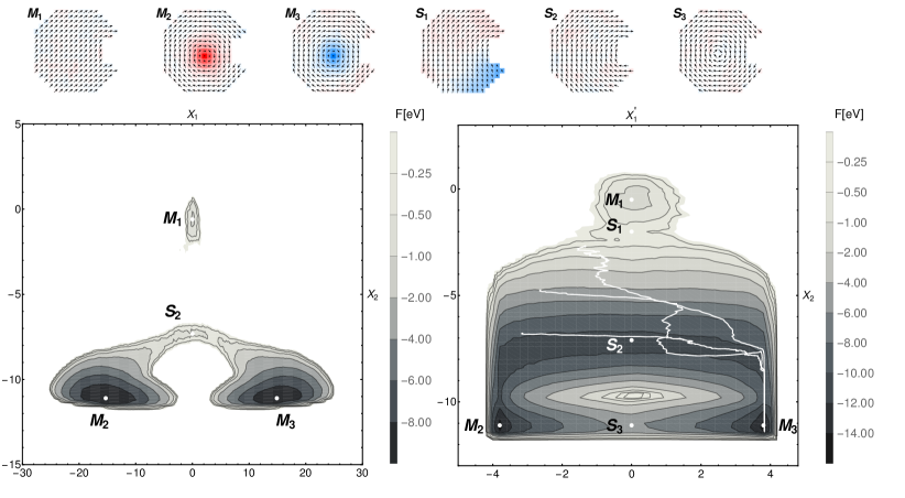
Figure 2: The map of the free energy as function of collective variables $X_{1}$, $X_{2}$ given by equations (4a,4b) (left panel) and free energy as function of the transformed variable $X_{1}^{\prime}$ (4a’) and $X_{2}$ (right panel). The starting configuration is in the point $\mathrm{M_{1}}$. Vortex state corresponds to global minima $\mathrm{M_{2}}$ and $\mathrm{M_{3}}$. The lowest saddle between minima $\mathrm{M_{2}}$ and $\mathrm{M_{3}}$ is labeled $\mathrm{S_{2}}$. The lowest energy barrier to climb to escape from local minimum $\mathrm{M_{1}}$ is defined by saddle point $\mathrm{S_{1}}$. The saddle point $\mathrm{S_{3}}$ is a numerical artefact related to finite discretization of the magnetization field $\mathbf{M}$. White color on background indicates un-explored configuration space. Note that region in vicinity of $\mathrm{M_{1}}$ is not connected to the rest of the map on the left panel.

The choice of the collective variable is crucially important for the success of the technique. As collective variables we took:

$$X_{1} =\int M_{z}\left(\partial_{x}M_{y}-\partial_{y}M_{x}\right)d\Omega$$ (4a)

$$X_{2} =\int r_{x}(M_{y}-\bar{M}_{y})-r_{y}(M_{x}-\bar{M}_{x})d\Omega$$ (4b)

Here $\bar{M}_{x}$ stands for average value $\bar{M}_{x}=1/\Omega\int M_{x}d\Omega$. The form of collective variables $X_{1}$ resembles definition of helicity in fluid dynamics. The helicity of the vector field $\mathbf{v}$ is defined as $\mathbf{v}\cdot\nabla\times\mathbf{v}$. The collective variable $X_{1}$ catches polarization of the vortex core multiplied by sense of rotation in the core region. Collective variable $X_{2}$ reflects circulation of the spin field and its absolute value is higher for closed circular spin textures. The negative sign of $X_{2}$ corresponds to clock-wise rotation of magnetization in nanodot. Subtraction of averages in formula (4b) guarantees invariance of the $X_{2}$ variable with respect to the choice of origin for $\mathbf{r}$ coordinate system. Clock-wise rotation is energetically favored by external field as explained in our previous work PRB-Cambel ; PRB-Tobik . Initial states are characterized by $X_{1}=0$, because the initial spin configuration is in-plane for each spin. The absolute value $|X_{2}|$ is small for states without vortex. The vortex state is characterized by negative value of $X_{2}$ (because of clockwise rotation of spin field lines in vortex states) and positive or negative value of $X_{1}$ depending on polarity of the nucleated vortex. It can be seen that the variables $X_{1},X_{2}$ can well distinguish between the initial and final states (Figs. 1, 2). Importantly, both CV correspond to slow degrees of freedom since their change requires a massive reorganization of the spin configuration.

Our implementation of metadynamics is based on the Metropolis-Hastings algorithm of MC sampling methodMetropolis ; Hastings . The history (time) dependent potential is chosen to have a form of sum of the Gaussians centered around previously stored collective variables configurations:

$$V(\mathbf{X})=\sum_{i=1}^{T}\mathrm{V_{0}}\,\exp\left(-\frac{|\mathbf{X}-\mathbf{X_{i}}|^{2}}{\sigma_{X}^{2}}\right).$$ (5)

The potential (5) is calculated in each step and is added to the total energy $E$ in equation (Free-energy landscapes in magnetic systems from metadynamics). The summation index $i$ runs over all stored configurations and $\mathbf{X}=(X_{1},X_{2})$ stands for collective variables. The amplitude of added Gaussians $V_{0}$ was set 0.06eV and standard deviation $\sigma_{X}$ in $(X_{1},X_{2})$ space was 0.03 (in arbitrary units after suitable rescaling of the variables, see Figs. 1,2). The time-dependent energy enters decision strategy for acceptance of new configuration as in standard Metropolis-Hastings algorithm:

$$P(\mathbf{X}_{n+1},\mathbf{X}_{n})=\left\{\begin{array}[]{ll}\exp\left(-\frac{E_{n+1}-E_{n}}{k_{B}T}\right)&\text{for }E_{n+1}>E_{n}\\ 1&\text{otherwise}\end{array}\right..$$ (6)

The local MC steps were realized by changing one spin per step. The change had to be small in order to keep the acceptance ratio reasonable. This was done by adding to randomly chosen spin a vector with amplitude 0.1 and with uniform probability distribution on the sphere using the Marsaglia algorithm Marsaglia . Afterwards the spin amplitude was renormalized to one. The temperature of T=300K was used in our simulations.

The values of collective variables were stored with frequency of 100 steps. This choice improves the performance of metadynamics in several respects. It improves diffusivity in the configuration space of collective variables $\mathbf{X}$, at the same time allows to use Gaussians with larger spread value $\sigma_{X}$, and finally makes the summation in equation (5) faster reviews . In order to further speed-up this summation, we used k-d tree data structure kd-tree to store visited configurations. The k-d tree allows efficient storage of vectors and subsequent efficient finding of vectors within prescribed range. The summation of Gaussians in equation (5) was reduced within rectangle with Manhattan distance $5\sigma_{X}$ from the actual value of collective variables $\mathbf{X}$.

The results of simulation of the modelled system in various magnetic configurations is shown in the Figs. 1 and 2. The nanodot is disk with 70 nm diameter. The removed sector has 1/3 of radius with opening angle of $45^{\circ}$. The constituting material was Permalloy with saturation magnetization $M_{s}=8.6\times 10^{5}\,A/m$, and exchange constant $A=1.3\times 10^{-11}\,J/m^{3}$. The magnetic nanodot was discretized to $N=324$ magnetic moments $\vec{s}$, each of them having 2 degrees of freedom. This Pacman-like (PL) nanodot was also subject of our previous studies PRB-Cambel ; PRB-Tobik ; SciRep-Tobik . It was identified earlier that this system has two modes of vortex nucleationPRB-Tobik . One mode is characterized by transition from the C-state (configuration M1 in Fig. 1) to vortex state (configuration M2 or M3). Second mode is a transition from initial S-state (configuration M1 in Fig. 2) to vortex state (configuration M2 or M3). These two transitions (C-state to vortex or S-state to vortex, respectively) differ in the robustness of the vortex polarity control with respect to out-of-plane magnetic fieldPRB-Tobik and to temperatureSciRep-Tobik .

The initial states were prepared by damped zero temperature LLG dynamics by slowly decreasing external field from high value of 200mT to 30mT (C state) or to 40mT respectively (in case of S state). The angle between PL-nanodot axis of symmetry and applied magnetic field $\mathbf{H_{eff}}$ is $60^{\circ}$ for the C-state and $30^{\circ}$ for the S-state. The value of external magnetic field was fixed during metadynamics simulation. Initial states had no out-of plane magnetization. The system should undergo spontaneous symmetry breaking (nucleation of vortex) if the external field is decreased by 5mTPRB-Tobik . The initial states thus represent relatively shallow local minima.

The calculated free energy as function of collective variables (4a) and (4b) for the C-state is shown in the Fig. 1. The highest energy point to pass from $\mathrm{M_{1}}$ to minimum $\mathrm{M_{2}}$ is $\mathrm{S_{1}}$. The symmetry related lowest energy path to minimum $\mathrm{M_{3}}$ has the highest energy point at the saddle point $\mathrm{S_{2}}$. The symmetry in $X_{1}$ variable is already broken at the saddle points. The height of barrier to overcome from $\mathrm{M_{1}}$ to $\mathrm{M_{2}}$ or $\mathrm{M_{3}}$ is 1.8eV, barrier from $\mathrm{M_{2}}$ or $\mathrm{M_{3}}$ to $\mathrm{M_{1}}$ is 11.8eV. We note that the FES reconstructed with the simple version of metadynamics contains some numerical noise and the accuracy could be further improved by employing more sophisticated sampling techniques such as e.g. well-tempered metadynamics algorithm PRL_Barducci . The time evolution of energy and CV is shown in Fig. 1 in supplemental materialsupplement .

In the Fig. 2 we show the free energy profile for the metadynamics starting from the S-state ($\mathrm{M_{1}}$) which represents a shallow local minimum. The minimum $\mathrm{M_{2}}$ ($\mathrm{M_{3}}$) corresponds to clockwise vortex with positive (negative) polarity and the saddle $\mathrm{S_{2}}$ is C-like state. In this figure there are two panels with free energy map. The left panel shows the local minimum $\mathrm{M_{1}}$, disconnected from the rest of the map, since after leaving the high-energy initial state $\mathrm{M_{1}}$ the dynamics does not return to this region anymore. The time evolution of energy and CV is show in Fig. 2 in supplemental materialsupplement . The free energy landscape thus can be reliably reconstructed only in the vicinity of the deep global minima $\mathrm{M_{2}}$, $\mathrm{M_{3}}$ and the lowest saddle point between them $\mathrm{S_{2}}$. Because the full configuration space including all three minima $\mathrm{M_{1}},\mathrm{M_{2}},\mathrm{M_{3}}$ has too big volume we were not able to fill the configuration space with Gaussians in reasonable time and connect the minima $\mathrm{M_{1}}$ to $\mathrm{M_{2}}$ and $\mathrm{M_{3}}$. Therefore the region of the starting local minimum $\mathrm{M_{1}}$ is not on the same energy level as global minima $\mathrm{M_{2}}$, $\mathrm{M_{3}}$.

To circumvent this obstacle we decided to use new collective variable $X_{1}^{\prime}$ given by equation:

$$X_{1}^{\prime}=4\tanh\frac{X_{1}}{4}.$$ (4a’)

The reason for this transformation is to shrink configuration space for large values of $X_{1}$ and thus speed up filling of the global minima basins. The reconstructed free energy landscape is shown in the right panel of Fig. 2. The time evolution of energy and transformed CV is shown in Fig. 3 in supplemental materialsupplement . The topology of the free energy surface is different with respect to the previous case. There are two more saddle points in the free energy map $F(X_{1}^{\prime},X_{2})$ denoted as $\mathrm{S_{1}}$ and $\mathrm{S_{3}}$. The saddle $\mathrm{S_{3}}$ separates minima $\mathrm{M_{2}}$ and $\mathrm{M_{3}}$ in the region of configuration space with large value of chirality $X_{2}$. It corresponds to process, where the vortex core is shrunk to zero and then core is created again, but with opposite sign of helicity. This process is, however, an artifact of the numerical treatment of the continuous micro-magnetic model and should not happen in the continuum limit, because the vortex is topologically protected state. However, atomic nature of materials permits vortex destruction by shrinking the vortex core to zero, but the true energy barrier is probably much higher then our simulation shows. Note that a systematic study of the influence of mesh discretization was done in the case of skyrmion PRB_Klaui . The free energy profile along line $X_{1}=0$ is shown in the Fig. 4 in Supplemental Material supplement . The free energy barrier to escape from minimum $\mathrm{M_{1}}$ via the saddle point $\mathrm{S_{1}}$ is 1.0eV. Minima $\mathrm{M_{2}}$ and $\mathrm{M_{3}}$ are separated by energy barrier 9.1eV at saddle point $\mathrm{S_{2}}$. The free energy difference between saddle points $\mathrm{S_{1}}$ and $\mathrm{S_{2}}$ is 10.2eV.

A peculiar feature of the free energy (Fig. 2) map is the existence of a common saddle point $\mathrm{S_{1}}$ which defines the lowest energy barrier between initial in-plane magnetization and both final vortex states. The region between saddles $\mathrm{S_{1}}$ and $\mathrm{S_{2}}$ is region with substantial energy decrease without necessity to break the symmetry in $X^{\prime}_{1}$ variable. When the system reaches saddle point $\mathrm{S_{2}}$, further decrease of the energy is possible only if the symmetry of the collective variable $X^{\prime}_{1}$ is broken and the vortex polarity chooses sign. It was argued earlier that this kind of topology of the energy landscape induces breaking of symmetry in spin dynamicsSciRep-Tobik . The energy gradient in the region between $\mathrm{S_{1}}$ and $\mathrm{S_{2}}$ defines an effective field around which magnetization precesses (see equations (2) and (3)). The direction of the precession is given by gyro-magnetic moment which has a negative sign for electrons. Thus precession during the descent in energy between saddle points $\mathrm{S_{1}}$ and $\mathrm{S_{2}}$ breaks the symmetry of the vortex polarization sign. To demonstrate this idea we have simulated several times the evolution of the magnetization starting from various configurations between saddle points $\mathrm{S_{1}}$ and $\mathrm{S_{2}}$ (see also our videosupplement ). Our calculations were performed with use of open software OOMMFOOMMF . The dynamics was modeled by Landau-Lifshitz-Gilbert equation with Langevin term OOMMF-Lemcke . We have used damping coefficient $\alpha=0.1$ and the amplitude of random fluctuating field was corresponding to temperature T=300K. The trajectories in configuration space are shown in Fig. 2 (right panel) by white lines. The precession drift towards one of the two possible vortex states is of course not observable in simulations, which do not contain precession term. In this respect simulations using just energy functional like e.g. Metropolis - Hastings MC and simulations based on Landau-Lifshitz dynamics with Langevin term differ. While MC is purely stochastic process and therefore the choice of the minima $\mathrm{M_{2}}$ and $\mathrm{M_{3}}$ is random, the Landau-Lifshitz dynamics carries system towards minimum $\mathrm{M_{3}}$ due to precession. With the use of our approach we thus gained additional argument supporting dynamical origin of the symmetry breaking mechanism in cases of particular topology of the FES. These phenomena are likely to be observed also in other magnetic systems. We believe that this precession drift during energy descent was already observed in magnetic dots similar in shape to ours experimentally Im-NPG as well as numerically JMMM-Li .

We note that the design of CV for our system was inspired by the knowledge of its initial and final states PRB-Cambel ; PRB-Tobik . The evolution during the metadynamics exploration of the FES was smooth indicating that the chosen set of CV is appropriate and complete. However, it is likely that for different systems (e.g. those allowing skyrmions) a different choice of CV might be more appropriate.

To summarize, we have implemented the metadynamics algorithm to a branch of physics, where to our knowledge, this method was not used before. This tool can enable new type of calculations in micro-magnetism, e.g. to map the free energy landscapes and determine the relevant barriers at finite temperature as well as to search for new magnetic textures. We also note that our approach may open new possibilities of magnetization control in magnetic nano-devices.

References

- (1) H. Pelzer, E. Wigner, Z. Phys. Chem. B 15, 445 (1932).
- (2) H.A. Kramers, Physica 7, 284 (1940).
- (3) J.S. Langer, Ann. Phys. 54, 258 (1969).
- (4) L. Néel, Ann. Geophys. 5, 99 (1949).
- (5) W. F. Brown, Jr ., Phys. Rev. 130, 1677 (1963).
- (6) H.B. Braun, Phys. Rev. Lett. 71, 3557 (1993).
- (7) W.T. Coffey and Y.P. Kalmykov, J. Appl. Phys. 112, 121301 (2012).
- (8) G. Mills and H. Jonsson, Phys. Rev. Lett. 72, 1124 (1994).
- (9) G. Henkelman, B.P. Uberuaga, and H. Jónsson, J. Chem. Phys. 113, 9901 (2000).
- (10) P.F. Bessarab, V.M. Uzdin, and H. Jónsson, Comp. Phys. Comm. 196, 335 (2015).
- (11) G.M. Torrie and J.P. Valleau, J. Comp. Phys. 23, 187 (1977).
- (12) A. Ferrenberg and R. Swendsen, Phys. Rev. Lett. 61, 2635 (1988).
- (13) For example see reviews: O. Valsson, P. Tiwary, and M. Parrinello, Annual Review of Physical Chemistry 67, 159 (2016), Ch. Delago and P.G. Polhuis, Adv. Polym. Sci. 221, 167 (2009), A. Barducci, M. Bonomi, and M. Parrinello, Comput. Mol. Sci. 1, 1 (2011).
- (14) A. Laio and M. Parrinello, PNAS 99, 12562 (2002).
- (15) G. Bussi, A. Laio, and M. Parrinello, Phys. Rev. Lett. 96, 090601 (2006).
- (16) A. Laio and F.L. Gervasio, Rep. Prog. Phys. 71, 126601 (2008).
- (17) J. Tóbik, V. Cambel, and G. Karapetrov, Sci. Rep. 5 ,12301 (2015).
- (18) A.N. Bogdanov and U.K. Rößler, Phys. Rev. Lett. 87, 037203 (2001).
- (19) F.N. Rybakov, A.B. Borisov, S. Blügel, and N.S. Kiselev, Phys. Rev. Lett. 115, 117201 (2015).
- (20) V. Cambel and G. Karapetrov, Phys. Rev. B 84, 014424 (2011).
- (21) J. Tóbik, V. Cambel, and G. Karapetrov, Phys. Rev. B 86, 134433 (2012).
- (22) N. Metropolis, A.W. Rosenbluth, M.N. Rosenbluth, A.H. Teller, E. Teller, J. Chem. Phys. 21, 1087 (1953).
- (23) W.K. Hastings, Biometrika 57, 97 (1970).
- (24) G. Marsaglia, Ann. Math. Stat. 43, 645 (1972).
- (25) Bentley, J. L. ”Multidimensional binary search trees used for associative searching”. Communications of the ACM. 18 (9): 509 (1975).
- (26) A. Barducci, G. Bussi, and M. Parrinello, Phys. Rev. Lett. 100, 020603 (2008).
- (27) See our supplementary material.
- (28) A. De Lucia, K. Litzius, B. Krüger, O.A. Tretiakov, and M. Kläui, Phys. Rev. B 96, 020405(R) (2017).
- (29) We have implemented metadynamics as a new time evolver module into software OOMMF. M. J. Donahue and D. G. Porter , OOMMF User’s Guide, Version 1.0, Interagency Report NISTIR 6376, National Institute of Standards and Technology, Gaithersburg, MD (Sept 1999).
- (30) Langevin-like dynamics implemented by O. Lemcke in module thetaevolve. It follows theoretical paper: J.L. García-Palacios and F.J. Lázaro, Phys. Rev. B 58, 14937 (1998).
- (31) M.Y. Im, P. Fisher, H.S. Han, A. Vogel, M.S. Jung, W. Chao, Y.S. Yu, G. Meier, J.I. Hong, K.S. Lee, NPG Asia Materials 9, e348 (2017).
- (32) J. Li, Y. Wang, , J. Cao, X. Meng, F. Zhu, Y. Wu, and R. Tai, J. Magn. Magn. Mater. 435, 167 (2017).