Lasso Meets Horseshoe: A Survey
Abstract
The goal of this paper is to contrast and survey the major advances in two of the most commonly used high-dimensional techniques, namely, the Lasso and horseshoe regularization. Lasso is a gold standard for predictor selection while horseshoe is a state-of-the-art Bayesian estimator for sparse signals. Lasso is fast and scalable and uses convex optimization whilst the horseshoe is non-convex. Our novel perspective focuses on three aspects: 1. theoretical optimality in high-dimensional inference for the Gaussian sparse model and beyond, 2. efficiency and scalability of computation and 3. methodological development and performance.
keywords:
*[enumerate]label=() \endlocaldefs
1 Introduction
High-dimensional predictor selection and sparse signal recovery are routine statistical and machine learning practices. There is a vast and growing literature focusing on computational aspects of large scale inference problems. Whilst this area is too large to review here, we revisit two popular sparse parameter estimation techniques, the Lasso (Tibshirani,, 1996) and the horseshoe estimator (Carvalho et al.,, 2010). Specifically, we focus on three areas: performance in high-dimensional data, theoretical optimality and computational efficiency.
Sparsity relies on the property of a few large signals among many (nearly) zero noisy observations. A common goal in high-dimensional inference is to recover the low-dimensional signals observed in noisy observations. This problem encompasses four related areas:
-
1.
Estimation of the underlying sparse parameter vector.
-
2.
Multiple testing where the # tests is much larger than the sample size, .
-
3.
Regression subset selection where # of covariates is far larger than .
-
4.
Out-of-sample prediction.
There are a rich variety of methodologies for high-dimensional regularization which implicitly or explicitly penalize model dimensionality. Lasso (Least Absolute Shrinkage and Selection Operator) produces a sparse estimate by constraining the norm of the parameter vector. Lasso’s widespread popularity is due to a multitude of factors, in particular due to the computational efficiency of the least angle regression (LARS) (Efron et al.,, 2004) or the simple coordinate descent approaches of Friedman et al., (2007), and its ability to produce a sparse solution, with optimality (oracle) properties for both estimation and variable selection (vide Bühlmann & van de Geer,, 2011; James et al.,, 2013; Hastie et al.,, 2015). Table 1, adapted from Tibshirani, (2014), gives a list of popular regularization methods based on Lasso.
| Method | Authors \bigstrut |
|---|---|
| Adaptive Lasso | Zou, (2006) \bigstrut[t] |
| Compressive sensing | Donoho, (2006); Candes, (2008) |
| Dantzig selector | Candes & Tao, (2007) |
| Elastic net | Zou & Hastie, (2005) |
| Fused Lasso | Tibshirani et al., (2005) |
| Generalized Lasso | Tibshirani & Taylor, (2011) |
| Graphical Lasso | Friedman et al., (2008) |
| Grouped Lasso | Yuan & Lin, (2006) |
| Hierarchical interaction models | Bien et al., (2013) |
| Matrix completion | Candès & Tao, (2010); Mazumder et al., (2010) |
| Multivariate methods | Jolliffe et al., (2003); Witten et al., (2009) |
| Near-isotonic regression | Tibshirani et al., (2011) |
| Square Root Lasso | Belloni et al., (2011) |
| Scaled Lasso | Sun & Zhang, (2012) |
| Minimum concave penalty | Zhang, (2010) |
| SparseNet | Mazumder et al., (2012) \bigstrut[b] |
Bayes procedures, on the other hand, can be classified into two categories: two-groups model or spike-and-slab priors (Johnstone & Silverman,, 2004; Efron,, 2008, 2010; Bogdan et al.,, 2011; Castillo & van der Vaart,, 2012) and global-local shrinkage priors (Carvalho et al.,, 2009, 2010; Griffin & Brown,, 2010; Armagan et al.,, 2011, 2013a; Polson & Scott,, 2010b), with the horseshoe prior (Carvalho et al.,, 2010) being one of the most popular methods. The first class, spike-and-slab prior, places a discrete mixture of a point mass at zero (the spike) and an absolutely continuous density (the slab) on each parameter. The second entails placing absolutely continuous shrinkage priors on the entire parameter vector that selectively shrinks the small signals. Table 2 provides a sampling of a few continuous shrinkage priors popular in the literature. Both these approaches have their own advantages and caveats, which we discuss in turn. A key duality is that the point estimate from a regularization approach can be interpreted as Bayesian mode of the posterior distribution under an appropriate shrinkage prior.
| Global-local shrinkage prior | Authors \bigstrut |
|---|---|
| Normal Exponential Gamma | Griffin & Brown, (2010) \bigstrut[t] |
| Horseshoe | Carvalho et al., (2010, 2009) |
| Hypergeometric Inverted Beta | Polson & Scott, (2010a) |
| Generalized Double Pareto | Armagan et al., (2011) |
| Generalized Beta | Armagan et al., (2013a) |
| Dirichlet–Laplace | Bhattacharya et al., (2015) |
| Horseshoe+ | Bhadra et al., (2017a) |
| Horseshoe-like | Bhadra et al., (2017b) |
| Spike-and-Slab Lasso | Ročková & George, (2016) |
| R2-D2 | Zhang et al., (2016) \bigstrut[b] |
| Inverse-Gamma-Gamma | Bai & Ghosh, (2017) \bigstrut[b] |
Both Lasso and horseshoe procedures come with strong theoretical guarantees for estimation, prediction and variable selection. Both procedures possess asymptotic oracle properties, i.e. identify the true non-zero coefficients as well as achieve the optimal estimation rate. The behavior of the Lasso estimator in terms of the risk properties has been studied in depth and has resulted in many methods aiming to improve certain features (see Table 1). On the other hand, horseshoe and other global-local priors have been shown to achieve optimality in variable selection, estimation and prediction, that we review in §4, although theoretical studies of the continuous shrinkage priors is still an active area.
The rest of the paper is organized as follows: Section 2 provides historical background for the normal means (a.k.a the Gaussian compound decision problem) and the sparse regression problems. Section 3 provides the link between regularization and optimization perspectives viewed through a probabilistic Bayesian lens. Section 4 compares and contrasts the statistical risk properties of Lasso and the horseshoe prior. Sections 5 and 6 discuss the issues of hyper-parameter selection and computational strategies. Section 7 provides two simulation experiments comparing the horseshoe prior with penalized regression methods for linear model and logistic regression with varying degree of dependence between predictors. We discuss applications of Lasso and the horseshoe in Section 8 and provide directions for future work in Section 9.
2 Sparse Normal Means, Regression and Variable Selection
2.1 Sparse Normal Means
Suppose that we observe data from the probability model for . Our primary inferential goal is to estimate the vector of normal means and a secondary goal is to simultaneously test if ’s are coming from a null distribution. We are interested in the sparse paradigm where a large proportion of the parameter vector contains zeros. The ‘nearly black’ (Donoho et al.,, 1992) regime occurs when the parameter vector lies in the set with the upper bound on the number of non-zero parameter values as .
A natural Bayesian solution for inference under sparsity is the two-groups model that puts a non-zero probability spike at zero and a suitable prior on the non-zero ’s (vide Appendix A). The inference is then based on the posterior probabilities of non-zero ’s based on the discrete mixture model. The two-groups model possesses a number of frequentist and Bayesian optimality properties. Johnstone & Silverman, (2004) showed that a thresholding-based estimator for under the two-groups model with an empirical Bayes estimate for the sparsity proportion attains the minimax rate in norm for for that are either nearly black or belong to an ball of ‘small’ radius. Castillo & van der Vaart, (2012) treated a full Bayes version of the problem and again found an estimate that is minimax in norm for mean vectors that are either nearly black or have bounded weak norm for .
2.2 Sparse Linear Regression
A related inferential problem is high-dimensional linear regression with sparsity constraints on the parameter vector . We are interested in the linear regression model:
where is a matrix of predictors and .
Our focus is on the sparse solution where and most of ’s are zero. Similar to the sparse normal means problem, our goal is to identify the non-zero entries of as well as estimate it. There are a wide variety of methods based on the penalized likelihood approach that solves the following optimization problem:
| (1) | ||||
| where |
Lasso uses an penalty, , and simultaneously performs variable selection while maintaining estimation accuracy. Another notable variant is the best subset selection procedure corresponding to the penalty . There has been a recent emphasis on non-concave separable penalties such as the minimax concave penalty or MCP (Zhang,, 2010) or SCAD (Fan & Li,, 2001), that act as a tool for variable selection and estimation. We discuss the penalization methods from a Bayesian viewpoint in the next section.
2.3 Variable Selection
Variable or predictor selection is intimately related to high-dimensional sparse linear regression. A sparse model provides interpretability, computational efficiency, and stability of inference. Lasso’s success has inspired many estimation methods that rely on convexity and sparsity in a penalized estimation framework. The ‘bet on sparsity’ principle (Hastie et al.,, 2009) dictates the use of methods favoring sparsity, as no method uniformly dominates when the true model is dense.
Remark 1.
The LAVA method by Chernozhukov et al., (2017) strictly dominates both Lasso and ridge in a ‘sparse+dense’ model. In fact, the LAVA estimator performs as well as Lasso in a sparse regime and as well as ridge (Tikhonov,, 1963) in a dense regime. This questions the validity of the ‘bet on sparsity’ principle. Although there is no exact analogue of LAVA in the Bayesian world, the one-group shrinkage priors share a common philosophy. The horseshoe-type priors are also designed to work when true has a few large entries and very many small non-zero entries and produces a ‘non-sparse’ estimator, but LAVA can recover both the dense and sparse components unlike horseshoe.
A parallel surge of Bayesian methodologies has emerged for sparse regression problems with an underlying variable selection procedure. Hierarchical Bayesian modeling proceeds by selecting a model dimension , selecting a random subset of dimension and a prior on . The prior can be written as in Castillo et al., (2015):
| (2) |
Bayesian approaches for sparse linear regression include George, (2000); George & Foster, (2000); Mitchell & Beauchamp, (1988); Ishwaran & Rao, (2005) and more recently Ročková & George, (2016), who introduce the spike-and-slab Lasso prior, where the hierarchical prior on the parameter and model spaces assumes the form:
| (3) |
where indexes the possible models, and , model the null and non-null ’s respectively using two Laplace priors with different scales. However, the spike-and-slab type priors lead to substantial computational challenges as exploring the full posterior using point mass mixture priors is prohibitive due to a combinatorial complexity of updating the discrete indicators and infeasibility of block updating of model parameters.
The continuous shrinkage priors alleviate this by using efficient Gibbs sampling scheme based on block-updating the model parameters. We also note that while full posterior sampling remains a computational hurdle for the spike-and-slab prior, point estimates such as posterior mean and posterior quantiles can be obtained using a polynomial-time algorithm as shown by Castillo & van der Vaart, (2012). Ročková & George, (2016) discuss the inefficiency of stochastic search algorithms for exploring the posterior even for moderate dimensions and developed a deterministic alternative to quickly find the maximum a-posteriori model. Here 1. increasing the efficiency in computation in the spike-and-slab model remains an active area of research (see, e.g., Ročková & George,, 2016) and 2. some complicating factors in the spike-and-slab model, such as a lack of suitable block updates, have fairly easy solutions for their continuous global-local shrinkage counterparts, facilitating posterior exploration.
Polson & Scott, (2010b); Carvalho et al., (2010); Polson & Scott, (2012b) introduced the ‘global-local’ shrinkage priors that adjust to sparsity via global shrinkage, and identify signals by local shrinkage parameters. The global-local shrinkage idea has resulted in many different priors in the recent past, with varying degrees of success in theoretical and numerical performance. We compare these different priors and introduce a recently proposed family of horseshoe-like priors in §3.3.
The estimators resulting from the one-group shrinkage priors are very different from the shrinkage estimator due to James & Stein, (1961), who showed that maximum likelihood estimators for multivariate normal means are inadmissible beyond two dimensions. The James–Stein estimator is primarily concerned about the total squared error loss, without much regard for the individual estimates. In problems involving observations lying far away on the tails this leads to ‘over-shrinkage’ (Carvalho et al.,, 2010). In reality, an ideal signal-recovery procedure should be robust to large signals. Connections between the global shrinkage of James–Stein and global-local shrinkage of the horseshoe are discussed in more details in §4.
3 Lasso and Horseshoe
Regularization requires the researcher to specify a measure of fit, denoted by and a penalty function, denoted by . From a Bayesian perspective, and correspond to the negative logarithms of the likelihood and a suitable prior distribution, respectively. While regularization leads to an optimization problem of the form
| (4) |
the probabilistic approach leads to a Bayesian hierarchical model
| (5) |
For appropriate and , the solution to (4) corresponds to the posterior mode of (5), , where denotes the posterior density. The properties of the penalty are then induced by those of the prior. For example, regression with a least squares log-likelihood subject to an penalty or ridge (Tikhonov,, 1963; Hoerl & Kennard,, 1970) corresponds to a Gaussian prior under the same observation distribution, and an penalty (Lasso) corresponds to a double-exponential prior (Tibshirani,, 1996).
One interpretation of Lasso and related penalties is that these are methods designed to perform selection, while ridge and related based methods perform shrinkage. Selection-based methods such as the Lasso are unstable in many situations, e.g., in presence of multi-collinearity in the design (Hastie et al.,, 2009, ch.3).
Although ‘shrinkage’ and ‘selection’ are closely related, we tend to distinguish between them in the following sense. Shrinkage methods such as the horseshoe prior shrink towards by thresholding the shrinkage weights that behave like posterior inclusion probabilities to achieve variable selection. It should be noted that the continuous nature of prior on ensures a lack of exact zeros in the posterior, which is often preferred over dichotomous models by some practitioners (Stephens & Balding,, 2009) as more realistic. This is unlike the Lasso that performs explicit selection by making some of estimates and producing a true sparse solution. Ultimately, both selection and shrinkage have their advantages and disadvantages.
3.1 Lasso Penalty and Prior
As discussed before, the classical Lasso-based point estimate is the same as the posterior mode under component-wise Laplace prior, and the mode inherits the optimal properties of Lasso. For example, the oracle inequality in Bühlmann & van de Geer, (2011, Eq. (2.8), Th. (6.1)) states that with a proper choice of of order , the mean squared prediction error of Lasso is of the same order as if one knew active set ), up to and a compatibility constant . The compatibility (or restricted eigenvalue) constant reflects the compatibility between the design matrix and the norm of , and is defined as follows (Bühlmann & van de Geer,, 2011, Eq (6.4)):
Definition 2.
(Compatibility Condition). For and , let (with similar notation for ), and let . Then the compatibility condition is satisfied for the design for the true support set , if letting one has,
The constant is called the compatibility (or restricted eigenvalue) constant.
Lasso also exhibits other desirable properties such as computational tractability, consistency of point estimates of for suitable , and optimality results on variable selection.
3.2 Bayesian Lasso and Elastic Net
As discussed before, the posterior mean under the double-exponential prior, which is the Bayes estimate under squared error loss, does not satisfy the optimality properties of the posterior mode under the double-exponential prior (i.e., the Lasso). Along these lines, Castillo et al., (2015) argue that the Lasso is essentially non-Bayesian, in that the “full posterior distribution is useless for uncertainty quantification, the central idea of Bayesian inference.” Castillo et al., (2015) provide theoretical result that the full Lasso posterior does not contract at the same speed as the posterior mode.
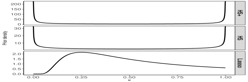
Thus, there are a number of caveats related to the use of a double-exponential prior for the general purposes of shrinkage. An important example is found in how it handles shrinkage for small observations and robustness to the large ones. This behavior is described by various authors, including Polson & Scott, (2010b); Datta & Ghosh, (2013), and motivates the key properties of global-local priors. Figure 1(a) provides profile plots as a diagnostic of shrinkage behavior for different priors.
For correlated predictors, Zou & Hastie, (2005) proposed a family of convex penalties called ‘elastic net’, which is a hybrid between Lasso and ridge. The penalty term is , where
Both Lasso and elastic net facilitate efficient Bayesian computation via a global-local scale mixture representation (Bhadra et al.,, 2016b). The Lasso penalty arises as a Laplace global-local mixture (Andrews & Mallows,, 1974), while the elastic-net regression can be recast as a global-local mixture with a mixing density belonging to the orthant-normal family of distributions (Hans,, 2011). The orthant-normal prior on , given hyper-parameters and , has a density function with the following form:
| (6) |
3.3 Horseshoe Penalty and Prior
The horseshoe prior is a continuous shrinkage rule for sparse signal recovery. Here we discuss the motivation behind the horseshoe prior for the Gaussian sequence model as it was developed in Carvalho et al., (2010), but note that it is applicable to sparse signal recovery in regression models and beyond, as we discuss in §4.4. Consider the normal means model: , . The horseshoe prior for , given a global shrinkage parameter , is given by the hierarchical model
| (7) |
As discussed before, the spike-and-slab prior or the two-groups model (vide Appendix A) with two dedicated components for separating noise and signal is a natural Bayesian solution but it leads to substantial computational burden. The horseshoe prior takes a different approach: instead of placing a prior on the model space to yield a sparse estimator, it models the posterior inclusion probabilities directly. To see this, note that the posterior mean under the horseshoe prior can be written as a linear function of the observation:
| (8) |
The name ‘horseshoe’ arises from the shape of the beta prior density of the shrinkage weights . A comparison with the posterior mean obtained under the two-groups model reveals that the shrinkage weights perform the same function as the posterior inclusion probability for recovering a sparse signal. Since the shrinkage coefficients are not formal Bayesian posterior quantities, we refer to them as ‘pseudo posterior inclusion probabilities.’
Carvalho et al., (2010) provided strong numerical evidence that the shrinkage weights from a one-group prior accurately approximates the inclusion probabilities under a two-groups model, and used this property to construct a multiple testing rule. The thresholding rule rejects the null hypothesis if the shrinkage weight exceed . Datta & Ghosh, (2013) validated this theoretically by proving that the horseshoe multiple testing rule attains the Bayes oracle up to a multiplicative constant under a - additive loss.
The marginal likelihood after reparametrizing is: . The posterior density of identifies signals and noises by letting and respectively. Since the marginal likelihood is zero when , it does not help identify the signals. Intuitively, any prior that drives the probability to either extremities should be a good candidate for sparse signal reconstruction. The horseshoe prior, with an induced prior density on proportional to does exactly that: it cancels the term in the marginal likelihood and replaces it with to enable in the posterior. The horseshoe+ prior (Bhadra et al.,, 2017a) takes this philosophy one step further, by creating a -shaped Jacobian for transformation from to -scale. The double-exponential on the other hand, yields a prior that decays at both ends with a mode near , thus leading to a posterior that is neither good at adjusting to sparsity, nor at recovering large signals.
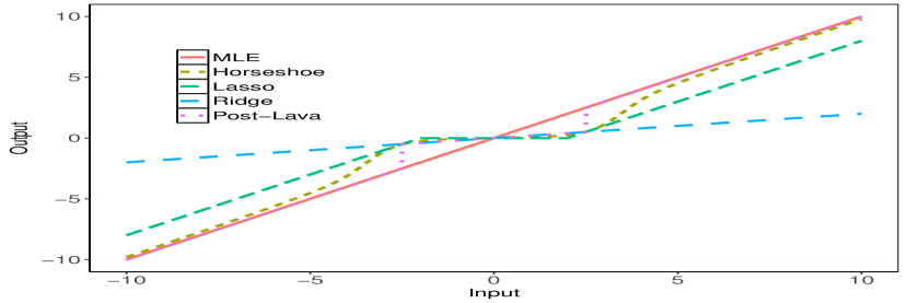
Figure 1(a) plots the prior density for the horseshoe, horseshoe+, and the Laplace priors. Figure 1(b) shows the resulting shrinkage function by plotting the input observations against the output estimates for horseshoe, horseshoe+, and Laplace priors, along with the maximum likelihood estimator (). Both Lasso and horseshoe shrink the small observations, but while horseshoe and horseshoe+ leave the large inputs unshrunk, Lasso shrinks them by a non-vanishing amount, resulting in a non-zero bias. We also plot the shrinkage function for the post-lava estimator (Chernozhukov et al.,, 2017) (vide Appendix C) which works well on dense+sparse signals, and has the robustness property lacking in Bayesian Lasso or the Laplace prior.
There are a number of closed-form results for the posterior distribution under a horseshoe prior. Although the prior density under the horseshoe prior does not admit a closed form, we can write the horseshoe posterior mean using the Tweedies’ formula , which is also the Bayes adjustment that provides an optimal bias-variance trade-off. For the horseshoe prior, Tweedies’ formula yields:
| (9) |
where is the bivariate confluent hypergeometric function (Gordy,, 1998). A similar formula is available for the posterior variance. This enables one to rapidly calculate the posterior mean estimator under the horseshoe prior via a ‘plug-in’ approach with estimated values of the hyper-parameter . We discuss the different approaches for handling in §5 and statistical properties of horseshoe posterior mean estimator and the induced decision rule in more details in § 4.
The horseshoe prior is a member of a wider class of global-local scale mixtures of normals that admit following hierarchical form (Polson & Scott,, 2010b):
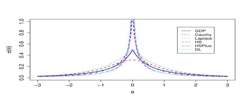
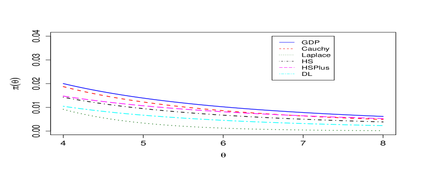
These priors are collectively called global-local shrinkage priors in Polson & Scott, (2010b), since they recover signals by a local shrinkage parameter and adapt to sparsity by a global shrinkage parameter. Table 2 provides a list of the popular and recent global-local shrinkage priors. A natural question is how do we compare these priors? It is known due to several authors (e.g., Polson & Scott,, 2010b; Bhadra et al.,, 2016a) that the key features of a global-local shrinkage prior is a peak at origin and heavy tails. An early example of such a prior was proposed by Cutillo et al., (2008) in the context of wavelet thresholding where a heavier tail was attained by modeling and where . We list a few popular global-local shrinkage priors along with their behavior near origin and the tails on Table 2, and a discussion of the recent extensions of global-local priors beyond the Gaussian model is deferred to § 8.
| Prior | Origin Behavior | Tails |
|---|---|---|
| Horseshoe | ||
| Horseshoe+ | ||
| Horseshoe-like | ||
| GDP | Bounded at origin | |
| () | () |
From a regularization view-point, one way to judge a prior is by the penalty it imposes on a likelihood (4), although in a strict Bayesian spirit, a prior should be evaluated based on the whole posterior, as shown by several authors including Castillo et al., (2015) and van der Pas et al., (2017). Although the horseshoe prior leads to optimal performance as a shrinkage prior, the induced penalty does not admit a closed form as the marginal prior is not analytically tractable. This poses a hindrance in learning via Expectation-Maximization or other similar algorithms. The generalized double Pareto prior of Armagan et al., (2011) admits a closed form solution, but it does not have an infinite spike near zero needed for sparse recovery. Motivated by this fact, Bhadra et al., (2017b) recently proposed the ‘horseshoe-like’ prior by normalizing the tight bounds for the horseshoe prior. Thus, the horseshoe-like prior attains a unique status within its class: it has a closed form marginal prior for , yet with a spike at origin and heavy tails and more importantly, admits a global-local scale mixture representation. The scale mixture representation supports both a traditional MCMC sampling for uncertainty quantification in full Bayes inference and EM/MM or proximal learning when computational efficiency is the primary concern.
Since the aim of designing a sparsity prior is achieving higher spike near zero while maintaining regularly varying tails, a useful strategy is to split the range of the prior into disjoint intervals: and , and aim for higher spike in one and heavier tail in the other. This leads to a class of ‘horseshoe-like’ priors with more flexibility in shape than any single shrinkage prior. We provide the general form of horseshoe-like priors and a key representation theorem. The proof that horseshoe-like prior is a scale mixture with Slash normal mixing density involves Frullani’s probabilistic identity (vide Jeffreys & Swirles,, 1972, pages 406-407), and to save substantial additional space we refer the readers to the proof in §5, Lemma 5.1 and Proposition 5.1 of Bhadra et al., (2017b).
- Horseshoe-like priors:
-
Bhadra et al., (2017b) have the following marginal prior density for :
(10) The general family of horseshoe-like priors can be constructed as a density split into disjoint intervals as follows:
(11) - Normal scale mixture:
-
The horseshoe-like prior (10) is a Gaussian scale mixture with a Slash Normal mixing density, which is in turn another Gaussian scale mixture of density, yielding the following representation theorem:
| Prior for | Prior for | Prior for |
|---|---|---|
| Horseshoe | ||
| Horseshoe+ | ||
| Double Exponential |
4 Statistical Risk Properties
4.1 Inadmissibility of MLE
We briefly discuss the Stein shrinkage phenomenon as it provides an useful insight into the development of global-local shrinkage estimators in high-dimensional problems. The James–Stein (JS) estimator is which is equivalent to the empirical Bayes estimate , under i.i.d. priors on and being the empirical Bayes estimate of from the data (Efron,, 2010). Thus, the James–Stein estimator corresponds to the Bayes risk of . We argue below that a global shrinkage rule such as the James–Stein estimator or regularization does not work in the sparse regime as it lacks local parameters for handling sparsity.
The story of shrinkage estimation goes back to the proof in Stein, (1956) that the maximum likelihood estimators for normal data are inadmissible beyond . James & Stein, (1961) proved that this estimator dominates the MLE in terms of the expected total squared error for every choice of , i.e. it outperforms the MLE no matter what the true is. To motivate the need for developing a local shrinkage rule, consider the classic James–Stein (JS) ‘global’ shrinkage rule, . The JS estimator uniformly dominates the traditional sample mean estimator, . For all values of the true parameter and for , we have the classical mean squared error (MSE) risk bound:
For sparse signal problem the standard James–Stein shrinkage rule, , performs poorly. This is best seen in the sparse setting for a -spike parameter value with coordinates at which has . Johnstone & Silverman, (2004) show that with risk at the origin. This leads to a bound (for )
The lower bound is the risk of an ‘ideal’ linear estimator . For an ‘ideal’ estimator, is known and is chosen to minimize the MSE, which gives
| (13) |
Theorem 5 of Donoho & Johnstone, (1995) states the following result, an oracle inequality for the James–Stein estimator:
Here, for the -spike parameter value has risk at least . This is nowhere near optimal. As Donoho & Johnstone, (1994) showed, simpler rules such as the hard-thresholding and soft-thresholding estimates given by and satisfy an oracle inequality. In particular, when the thresholding sequence is close to (universal threshold), these estimators attain the ‘oracle risk’ up to a factor of . Intuitively, this is not surprising as the high-dimensional normal prior places most of its mass on circular regions – and does not support sparse, spiky vectors. The James–Stein estimator was not built for sparse estimation and it is ambivalent to sparsity assumptions, but the shrinkage phenomenon in lower dimensional regime paves the way for building shrinkage rules for sparse regime, where one needs an additional ‘local’ shrinkage term to recover the signals.
4.2 Near minimax risk
The asymptotically minimax risk rate in for nearly black objects is given by Donoho et al., (1992) to be . Here means . Specifically, for any estimator , we have a lower bound ():
| (14) |
The minimax rate, which is a frequentist criteria for evaluating the convergence of point estimators to the underlying true parameter, is a validation criteria for posterior contraction as well. This result, due to Ghosal et al., (2000), showed that the minimax rate is the fastest that the posterior distribution can contract.
A key advantage of the horseshoe estimators is that they enjoy near-minimax rates in both an empirical Bayes and full Bayes approach, provided that the hyper-parameters or the priors are suitably chosen–as proved in a series of papers (van der Pas et al.,, 2014, 2016a, 2016c; van der Pas et al.,, 2017). Specifically, for , the horseshoe estimator achieves
| (15) |
van der Pas et al., (2014) showed that the near-minimax rate can be achieved by setting the global shrinkage parameter . In practice, is unknown and must either be estimated from the data or handled via a fully Bayesian approach by putting a suitable prior on . van der Pas et al., (2017) show that the theoretical optimality properties for the popular horseshoe prior holds true if the global shrinkage parameter is learned via the maximum marginal likelihood estimator (MMLE) or a full Bayes approach. Independently, van der Pas et al., (2016a) and Ghosh et al., (2017) showed that these optimality properties are not unique features of the horseshoe prior and they hold for a general class of global-local shrinkage priors. While the results of van der Pas et al., (2016a) apply to a wider class of priors, including the horseshoe+ prior (Bhadra et al.,, 2017a) and spike-and-slab Lasso (Ročková & George,, 2016), it is worth pointing out the difference between van der Pas et al., (2016a) and Ghosh et al., (2017). van der Pas et al., (2016a) prove ‘near-minimaxity’ under ‘uniform regular variation’ conditions on the prior on local shrinkage parameters for a general class of global-local priors that allow exponential tails. On the other hand, Ghosh et al., (2017) attain ‘exact’ minimaxity for ‘horseshoe-type’ priors under suitable conditions on the global parameter , but they allow only polynomial tails, leading to a narrower class.
4.3 Variable Selection: Frequentist and Bayes Optimality
Here we compare the relative performance of horseshoe and Lasso for multiple testing under the two-groups model and a - additive loss framework. One of the main reasons behind the widespread popularity of Lasso is the in-built mechanism for performing simultaneous shrinkage and selection. The horseshoe estimator, on the other hand, is a shrinkage rule that induces a selection rule through thresholding the pseudo posterior inclusion probabilities. Datta & Ghosh, (2013) proved that for large scale testing problems the horseshoe prior attains the oracle property while double-exponential tails prove to be insufficiently heavy, leading to a higher misclassification rate compared to the horseshoe prior. The main reasons behind the horseshoe prior’s optimality are the posterior density of shrinkage weights that concentrates near and and the adaptability of the global shrinkage parameter .
The posterior distribution under the horseshoe prior leads to a natural model selection strategy under the two-groups model. Carvalho et al., (2010) argued that the shrinkage coefficient can be viewed as a pseudo-inclusion probability and induces a multiple testing rule:
| (16) |
Under the two-groups model (24), and a - loss, the Bayes risk is
where and denote the probabilities of type 1 and type 2 error corresponding to the hypothesis respectively.
If we know the true proportion of sparsity and the parameters of the non-null distribution, we can derive a decision rule that is impossible to outperform in theory, which is called the Bayes oracle for multiple testing (Bogdan et al.,, 2011). The oracle risk serves as the lower bound for any multiple testing rule under the two-groups model and thus provides an asymptotic optimality criteria when the number of tests go to infinity. The framework of Bogdan et al., (2011) is:
| (17) |
where . Dropping the subscript from parameters for notational simplicity, the Bayes risk for the Bayes oracle under the above framework (17) is:
A multiple testing rule is said to possess asymptotic Bayes optimality under sparsity (ABOS) if it attains the oracle risk as . Bogdan et al., (2011) provided conditions for a few popular testing rules, e.g. Benjamini–Hochberg FDR controlling rule to be ABOS. Datta & Ghosh, (2013) first showed that the horseshoe decision rule (16) is also ABOS up to a multiplicative constant if is chosen suitably to reflect the sparsity, namely . The proof in Datta & Ghosh, (2013) hinges on the concentration of the posterior distribution near and , depending on the trade-off between signal strength and sparsity. In numerical experiments, Datta & Ghosh, (2013) also confirmed that the horseshoe decision rule outperforms the shrinkage rule induced by the double-exponential prior under various levels of sparsity. Although is treated as a tuning parameter that mimics in the theoretical treatment, in practice, is an unknown parameter. Several authors (Datta & Ghosh,, 2013; Ghosh et al.,, 2017, 2016; van der Pas et al.,, 2016c) have shown that usual estimates of adapts to sparsity, a condition that also guarantees near-minimaxity in estimation. Ghosh et al., (2016) extended the ABOS property to a wider class of global-local shrinkage priors, with conditions on the slowly varying tails of the local shrinkage prior. Ghosh et al., (2016) prove a stronger result, namely, the testing rule under a global-local prior attains the ABOS property exactly, when the global shrinkage parameter is of the same asymptotic order as the sparsity proportion .
4.4 Sparse Linear Regression
One of the major advantages of Lasso and other frequentist penalized methods is their theoretical optimality properties in the regression setting (Bühlmann & van de Geer,, 2011, e.g.), whereas similar results for Bayesian methods using shrinkage priors are relatively less common. We review extant theoretical results for Bayesian sparse regression covering both point-mass mixture and continuous shrinkage priors.
Point mass mixture priors: Arguably the most notable contribution is due to Castillo et al., (2015), who showed that the posterior under a point-mass mixture prior contracts at the optimal rate for sparse parameter recovery and prediction, given a suitable ‘compatibility’ condition on the design matrix is satisfied. Such compatibility conditions also govern oracle properties for Lasso-type methods, e.g. ‘irrepresentability’ and ‘mutual coherence’ conditions (Bühlmann & van de Geer,, 2011, vide Ch. 6) and (Zhao & Yu,, 2006). Similarly, for recovery under point-mass mixture priors, Castillo et al., (2015) define three local invertibility conditions on the regression matrix: (uniform compatibility in sparse vectors), (smallest scaled sparse singular value), and (mutual coherence), for recovery with respect to norm, norm and norm respectively. We define the irrepresentability and mutual coherence condition below.
First, suppose the sample covariance matrix is denoted by and the active set consists of first elements of as in Definition 2. One can partition the matrix as
where is the sub-matrix corresponding to the active variables. The strong irrepresentable condition for the variable selection consistency of Lasso is:
| (18) |
Zhao & Yu, (2006) illustrated the importance of strong irrepresentable condition on Lasso’s model selection performance by showing that the probability of selecting the true sparse model is an increasing function of the irrepresentability condition number, defined as:
| (19) |
The strongest of these conditions, mutual coherence (), is defined as:
| (20) |
Bühlmann & van de Geer, (2011) establishes the relationship between the different conditions (vide Fig. 6.1). Clearly, these optimality results carry over to the sparse normal means problem (‘sequence model’) where the design matrix is identity or to regression models with an orthogonal design matrix.
Continuous shrinkage priors: Polson & Scott, (2010b) point out that the one-group priors mimic Bayesian model averaging, where one achieves better predictive performance by averaging over models supported by data, without the computational burden. Several authors (Polson & Scott,, 2010b, 2012a; Datta & Ghosh,, 2015) have shown empirically horseshoe outperforms Lasso (as well as Bayesian model averaging) in terms of out-of-sample predictive sum-of-squares error.
Armagan et al., (2013b) proved posterior consistency in situation for commonly used shrinkage prior including generalized double Pareto and horseshoe-type priors under simple sufficient conditions, e.g. boundedness of the eigenvalues of and the number of non-zero elements . Under similar conditions, minimax posterior contraction rates for the Dirichlet-Laplace prior (Bhattacharya et al.,, 2015) can be extended to the regression coefficients . Non-trivial extension to the high dimensional setting is still an active area.
There are some recent developments on theoretical properties for predictive risk and variable selection properties of the horseshoe posterior under a orthogonal design matrix in situation. It is worth noting that there are two slightly different approaches for specifying the horseshoe prior. First, suppose a horseshoe prior is placed directly on the regression coefficient where under the model:
Tang et al., (2016) proposed the half-thresholding estimator,
where and are the posterior mean and the OLS solution, respectively, and showed this estimator achieves oracle property (variable selection consistency and optimal estimation) if local shrinkage priors have polynomial tails. On the other hand, Bhadra et al., (2016c) specifies the prior on a reparametrized follows (noting that and are one-to-one functions for a fixed design ):
| (21) |
Under assumption of an orthogonal design, Bhadra et al., (2016c) investigated Stein’s unbiased risk estimate for prediction, defined as for the horseshoe prior and proved that it leads to improved finite sample prediction risk, over ridge regression risk of .
Theorem 5.
As pointed out before, it remains to be settled whether stronger theoretical results hold for the horseshoe or other GL priors, e.g. whether oracle properties or minimaxity results under or norm carry over to horseshoe prior in the high-dimensional set-up under compatibility or coherence conditions on the design matrix as used by Bühlmann & van de Geer, (2011) and Castillo et al., (2015).
4.5 Uncertainty quantification
Reliable uncertainty quantification is a key challenge in high-dimensional inference. While some authors (e.g., Chatterjee & Lahiri,, 2011) observed that the Lasso-based estimates do not yield meaningful standard errors for the parameter estimates, Castillo et al., (2015) showed poor posterior contraction for the Bayesian Lasso. These results motivate Bayesian approaches with appropriately heavy-tailed priors that produce automatic and reliable uncertainty quantification.
Chatterjee & Lahiri, (2011) also proposed a bootstrap-based estimator for the limiting distribution of the Lasso that attains some non-uniform consistency. Similarly, Liu & Yu, (2013) argue that the bootstrap could be used. But these attempts are exposed to severe super-efficiency phenomena. In contrast, Zhang & Zhang, (2014) pioneered the idea to de-bias the Lasso for obtaining an asymptotic Gaussian limiting distribution for single coordinates or other low-dimensional parameters of interest. The de-biased Lasso is of the form:
The matrix is constructed from the node-wise Lasso, as also advocated by Van de Geer et al., (2014) or using a convex program as proposed by Javanmard & Montanari, (2014). In both approaches, exploiting KKT conditions for the node-wise Lasso or by construction, the norm is controlling the bias and is governing the variance of the de-biased or de-sparsified Lasso.
Although one can always get confidence sets for a fixed coefficient, arguably a more specific question here is whether these credible sets (marginal credible intervals or credible balls) have both the minimax radius and the correct coverage. At the heart of these results is the impossibility theorem by Li, (1989), that says one can not construct confidence sets to be both ‘honest’ and ‘adaptive’ uniformly for all , be it Bayesian or non-Bayesian. In particular, sparsity-adaptive credible sets can not be ‘honest’ (Nickl et al.,, 2013; Li,, 1989) in the sense that it is impossible to construct credible sets that have both their diameters adapt to the minimax rate for the unknown sparsity as well as provide nominal coverage probability over the full parameter space.
In the context of sequence models, as van der Pas et al., (2017) point out that since the horseshoe prior achieves adaptive posterior contraction at the near-minimax rate in (15) for nearly-black objects, one needs additional conditions, e.g., excessive bias-restriction (Belitser & Nurushev,, 2015) or self-similarity to ensure good coverage. In particular, they prove that credible balls provide uncertainty quantification up to a correct multiplicative factor, provided the sparsity proportion crosses the detectability threshold, . We refer the readers to Theorem 5 of van der Pas et al., (2017) for a precise statement concerning the coverage and size of the horseshoe credible sets. It appears that there is a trade-off between honesty and adaptation, and Bayesian procedures such as the horseshoe attain adaptation over honesty and de-biased methods offer honesty, often by sacrificing the optimal diameter criterion.
5 Hyper-parameters
Careful handling of the global shrinkage parameter is critical for success of the horseshoe estimator in a sparse regime as it captures the level of sparsity in the data (Carvalho et al.,, 2010; Datta & Ghosh,, 2013; van der Pas et al.,, 2016a). However, in nearly black situations a naïve estimate of could collapse to zero, and care must be taken to prevent possible degeneracy in inference. There are two main approaches regarding choice of : first, an empirical Bayesian approach that estimates from the data using a simple thresholding or maximum marginal likelihood approach (MMLE) and second, a fully Bayesian approach that specifies a hyper-prior on .
5.1 Marginal Likelihood
We first take a closer look at how affects the marginal likelihood under the horseshoe prior and the maximum marginal likelihood approach of van der Pas et al., (2017). We can write the marginal likelihood under the horseshoe prior after marginalizing out in (7) for from the model as:
Tiao & Tan, (1966) observe that the marginal likelihood is positive at , hence the impropriety of the prior of at the origin translates to the posterior. As a result, the maximum likelihood estimator of could potentially collapse to zero in very sparse problems (Polson & Scott,, 2010b; Datta & Ghosh,, 2013). In van der Pas et al., (2017), both the empirical Bayes MMLE and the full Bayes solution are restricted in the interval to preempt this behavior. To get the MMLE of using the approach of van der Pas et al., (2017), we first calculate the marginal prior of after integrating out in Equation (7):
The MMLE is then obtained as the maximizer of the marginal likelihood restricted to the interval :
The lower bound of the maximization interval prevents a degenerate solution of in the sparse case.
Handling is still an area of research: some papers (e.g., Carvalho et al.,, 2010; Datta & Ghosh,, 2013; Piironen & Vehtari,, 2017b) advocate using a full Bayes approach instead of a ‘plug-in’ maximum likelihood approach to avoid potential issues such as collapsing to zero. On the other hand, van der Pas et al., (2017) note the following:
“Piironen, Betancourt, Simpson and Vehtari close with a warning against the marginal maximum likelihood estimator. They are not the first to do so. We can only say that we have not noted problems, not in the theory and not in the simulations. We also prefer full Bayes, but the greater efficiency may weigh in the other direction.” (van der Pas et al.,, 2017, vide Rejoinder p. 1274).
In practice, the MMLE approach of van der Pas et al., (2017) achieves both theoretical optimality and good numerical performance. It is computed over the interval , which connects to the interpretation of as sparsity and prevents any computational issues.
5.2 Optimization and Cross-validation
In a recent paper, van der Pas et al., (2017) have investigated the empirical Bayes and full Bayes approach for , and have shown that the full Bayes and the MMLE estimators achieve the near minimax rate, namely , under similar conditions. For the full Bayes estimator, these conditions are easily seen to satisfied by a half-Cauchy prior truncated to the interval , which also does well in numerical experiments, both in ‘sparse’ and ‘less-sparse’ situations.
The MMLE estimator of van der Pas et al., (2017) outperforms the simple thresholding estimator given by:
Rather, the MMLE estimator can detect smaller non-zero signals, even those below the threshold , such as when .
A third approach could be treating as a tuning parameter and using a -fold cross-validation to select . As in the full Bayes and empirical Bayes approach, the cross-validated choice of can also converge to zero and care should be taken to avoid such situations. Yet another approach for handling was proposed by Piironen & Vehtari, (2017a), who have investigated the choice of for a linear regression model and have suggested choosing a prior for by studying the prior for , the effective number of non-zero parameters. When better prediction is desired, Bhadra et al., (2016c) suggest selecting by minimizing SURE, for which they provide an explicit form under the model in (21).
6 Computation
Over the last few years, several different implementations of the horseshoe prior for the normal means and regression models have been proposed. The MCMC based implementations usually proceed via block-updating , and using either a Gibbs, parameter expansion or slice sampling strategy. The first R package to offer horseshoe prior for regression along with Lasso, Bayesian Lasso and ridge was the monomvn package by Gramacy et al., (2010). In an unpublished technical report, Scott, (2010) proposed a parameter expansion strategy for the horseshoe prior and studied its effect on the autocorrelation of . Furthermore, Scott, (2010) pointed out that the solution to this lies in marginalizing over the local shrinkage parameter ’s. On a somewhat similar route, Makalic & Schmidt, (2016) uses a inverse-gamma scale mixture identity to construct a Gibbs sampling scheme for the horseshoe and horseshoe+ priors for linear regression as well as logistic and negative binomial regressions.
The horseshoe package implements the MMLE and truncated prior approaches for handling proposed in van der Pas et al., (2017). Hahn et al., (2016) proposed an elliptical slice sampler and argue that it outperforms Gibbs strategies for higher dimensional problems both in per-sample speed and quality of samples (i.e. effective sample size). The state-of-the-art implementation for the horseshoe prior in linear regression is by Bhattacharya et al., (2016) who used a Gaussian sampling alternative to the naïve Cholesky decomposition to reduce the computational burden from to . A very recent paper by Johndrow & Orenstein, (2017) claims to improve this even further by implementing a block update strategy but using a random walk Metropolis–Hastings algorithm on for block-updating . We provide a list of all implementations known to us on Table 5.
Bayesian methods using MCMC are sequential in nature. The methods are typically computation intensive, but one is able to perform probabilistic uncertainty quantification. However, sparse Bayesian methods including the horseshoe regression can be computed for , using parallel architecture of the latent variable representation to be able to retain the fully Bayesian nature via MCMC sampling. Terenin et al., (2018) implement a horseshoe-probit regression using GPU that takes minutes for calculations involving a design matrix of dimensions . If only point estimates are desired, of course Bayesian posterior modes can be computed as fast as penalized likelihood estimates (Bhadra et al.,, 2017b).
| Implementation (Package/URL) | Authors \bigstrut |
|---|---|
| R package: monomvn | Gramacy et al., (2010) \bigstrut[t] |
| R code in paper | Scott, (2010) |
| R package: horseshoe | van der Pas et al., (2016b) |
| R package: fastHorseshoe | Hahn et al., (2016) |
| Matlab code | Bhattacharya et al., (2016) |
| GPU accelerated Gibbs sampling | Terenin et al., (2018) |
| bayesreg + Matlab code in paper | Makalic & Schmidt, (2016) |
| Matlab code | Johndrow & Orenstein, (2017) \bigstrut[b] |
| R package:bayeslm | Hahn et al., (2017) |
7 Simulation Experiments
7.1 Effect of Correlated Predictors
As we discussed in §4.4, Lasso as well as Bayesian spike-and-slab priors can recover regression parameters under strong assumptions on the design matrix such as ‘irrepresentability’ or ‘mutual coherence’. As van der Pas et al., (2017) point out, such conditions are expected to be necessary for optimal recovery as in the context of spike-and-slab prior (Castillo et al.,, 2015).
For this simulation study, we follow the set-up in Zhao & Yu, (2006) closely. Let be the active set of predictors, and let . We simulate data with and with the sparse coefficient vector . The error variance was set to to obey the asymptotic properties of the Lasso.
We first draw the covariance matrix from and then generate design matrix from . Zhao & Yu, (2006) showed that the Strong Irrepresentability Condition (18) may not hold for such a design matrix. We generate such design matrices to obtain a range of different values. In our simulation studies the values in (19) for the 100 simulated designs were between . To see how the irrepresentability condition affects probability of selecting the correct model, simulations were conducted for each design matrix. We compare four different methods: two penalized likelihood methods: Lasso, SCAD (Smoothly Clipped Absolute Deviation) (Fan & Li,, 2001), and two Bayesian methods: horseshoe and Dirichlet–Laplace (Bhattacharya et al.,, 2015) in terms of percentage of these methods selecting the correct model. For model selection, we use the credible intervals for the horseshoe prior and -means clustering for the Dirichlet–Laplace prior, following the simulation study in Bhattacharya et al., (2015).
Like Zhao & Yu, (2006), we expect the Lasso to select the true model with a high probability when and poorly when , with the sharpest ascent around the origin. We also calculated the mutual coherence (20) number for the same design matrices to see the effect on these two methods. The numbers were between .
Figure 3 shows the percentage of correctly selected model as a function of the irrepresentable condition number, and mutual coherence for the four candidates: Lasso, SCAD, horseshoe and Dirichlet–Laplace. For this simulation experiment, Lasso’s model selection performance is dependent on the irrepresentability condition, deteriorating with decreasing . Surprisingly, the effect is weaker for SCAD as well as both the horseshoe and the Dirichlet–Laplace priors.
While the horseshoe almost always recovers the true sparse vector irrespective of , SCAD exhibits a high percentage (mean = , range = ). Since we have calculated mutual coherence for the same design matrices, in this set-up it does not affect the horseshoe prior’s variable selection, and its effect shows no clear pattern on any other candidates, apart from the Lasso.
7.2 Binary Response: Logistic Regression
We compare the performance of the horseshoe prior and Lasso for logistic regression for varying degree of dependence between the columns of a design matrix. We generated binary observations for the standard logistic regression. The true parameter where , is sparse and has 5 non-zero elements , and was set to . We set the covariance matrix as and then generate design matrix from for different values of . Since the original horseshoe prior was not designed to handle the logistic likelihood, we use the Gaussian approximation method by Piironen & Vehtari, (2017b), where they use a second-order Taylor expansion for the log posterior distribution. Piironen & Vehtari, (2017b) also propose the regularized horseshoe prior where one introduces an additional slab width to allow for shrinkage even on the extreme tails. Following the recommendations of Piironen & Vehtari, (2017b), we use the regularized horseshoe prior with a hyper-prior that corresponds to a slab. We use posterior draws per chain with the NUTS algorithm in Stan. For Lasso, we use the glmnet package in R with a -folds cross-validation.
To compare the two methods for classification and predictive accuracy, we train the models on 80% of the data, with the remaining as test set and average the results over random splits. We measure classification accuracy by the number of misclassified response ’s in test data. For predictive accuracy, we compare the mean log predictive density (MLPD) proposed in Gelman et al., (2014) as the mean of the computed log pointwise predictive density, defined as follows.
Let ; be the posterior draws from , and , be the test data, then MLPD is:
| (22) |
Figure 4(a) shows the average number of misclassified observations by horseshoe is a little lower than Lasso for all but two values of . For the same values of , Fig. 4(b) shows that the predictive accuracy under the horseshoe prior is a little better than the Lasso. We direct the readers to Piironen & Vehtari, (2017b) for a thorough comparison between the different variants of the horseshoe prior with Lasso for a few real data set as well as a synthetic data-set with a separable predictor.
(a)
(b)
8 Further Developments
8.1 Further Developments on Lasso
Since the inception of Lasso as a regularization method for linear regression in 1996, a great deal of extensions and applications have been proposed in the literature. The combined effect of convex penalty and sparsity of the final solution lead to huge computational gains by using powerful convex optimization methods on problems of massive dimensions. The coordinate descent approach (Friedman et al.,, 2007, 2010) is one particularly promising approach, that works by applying soft-threshold to the least-squares solution obtained on partial residuals, one at a time. The coordinate descent approach is flexible and easy and can be proved to converge to the solution as long as the log-likelihood and penalty are convex (Tseng,, 2001), paving the way for wide applicability of penalty in generalized linear models (GLM). The popular R package glmnet provides a nice and easy interface for applying Lasso and elastic-net penalty for a general sparse GLM.
8.2 Further Developments on Horseshoe
As discussed in Section 3.3, the horseshoe prior belongs to a wider class of global-local shrinkage priors (Polson & Scott,, 2010b) that are characterized by a local shrinkage parameter for recovering large signals and a global shrinkage parameter for adapting to overall sparsity. The class of global-local priors, although differing in their specific goals and design, exhibit some common features: heavy tails for tail-robustness and appreciable mass near zero for sparsity, leading to shared optimality properties.
Although the original horseshoe prior was developed for signal recovery with sparse Gaussian means, the idea of directly modeling the posterior inclusion probabilities and the use of normal-scale mixtures to facilitate sparsity is very flexible and can be easily generalized to a wider class of problems. Bhadra et al., (2016a) show that the horseshoe prior is a good candidate as a default prior for low-dimensional, possibly non-linear functionals of high-dimensional parameter and can resolve long-standing marginalization paradoxes for such problems. Bhadra et al., (2016c) show how to use global-local priors for prediction and provide theoretical and numerical evidence that it performs better than a variety of competitors including Lasso, ridge, PCR and sparse PLS.
Moving beyond Gaussianity, Datta & Dunson, (2016) re-discovered the Gauss hypergeometric prior for flexible shrinkage needed for quasi-sparse count data, with a tighter control on false discoveries. Piironen & Vehtari, (2017a) used a Gaussian approximation using a second-order Taylor expansion for the log-likelihood to apply the horseshoe prior in generalized linear models. Wang & Pillai, (2013) proposed a shrinkage prior based on a scale mixture of uniform for covariance matrix estimation. Peltola et al., (2014) applied the horseshoe prior for Bayesian linear survival regression for selecting covariates with highest predictive values. A sample of the many applications of the horseshoe prior is given in Table 6. Given the explosive growth of methodology in this area, we conjecture that the horseshoe prior would be regarded as a key tool for sparse signal recovery and as a default prior for objective Bayesian inference in many important problems.
| Application | Authors \bigstrut |
|---|---|
| Fadeout method for mean-field variational inference under non-centered parameterizations and stochastic variational inference for undirected graphical model. | Ingraham & Marks, (2016) \bigstrut[t] |
| Linear regression for Causal inference and Instrumental variable models | Hahn & Lopes, (2014); Hahn et al., (2016) |
| Multiclass prediction using DOLDA (Diagonally orthant Latent Dirichlet Allocation) | Magnusson et al., (2016) |
| Mendelian Randomization to detect causal effects of interest | Berzuini et al., (2016) |
| Locally adaptive nonparametric curve fitting with shrinkage prior Markov random field (SPMRF) | Faulkner & Minin, (2015) |
| Quasi-Sparse Count Data | Datta & Dunson, (2016) |
| Variable Selection under the projection predictive framework | Piironen & Vehtari, (2015) \bigstrut[b] |
| Dynamic shrinkage Process (dynamic linear model and trend filtering) | Kowal et al., (2017) |
| Logistic regression with horseshoe prior | Piironen & Vehtari, (2017b); Wei, (2017) |
| Tree ensembles with rule structured horseshoe regularization | Nalenz et al., (2018) |
| Bayesian compression for deep learning | Louizos et al., (2017) |
| Precision matrix estimation | Li et al., (2017) \bigstrut[b] |
9 Discussion
Sparsity can be achieved with Lasso and horseshoe regularization, a member of the class of global-local shrinkage priors. The horseshoe prior offers better computational efficiency than the Bayesian two-group priors, while still mimicking the inference and it outperforms the estimator based on Laplace prior, the Bayesian dual of Lasso. The intuitive reasons for better performance by the horseshoe prior are its heavy tails and probability spike at zero, which make it adaptive to sparsity and robust to large signals. A number of computing strategies have been proposed for both the Lasso and the horseshoe prior, based on variants of coordinate descent and MCMC respectively. We have outlined the distinct algorithmic implementations in §6 and Table 5. Since the goal of Lasso-based estimator is to produce a point estimate, rather than samples from the full posterior distribution of the underlying parameter, Lasso-based methods are typically faster than the horseshoe and related shrinkage priors.
The lack of speed can be overcome easily by employing a strategy based on expectation-maximization or proximal algorithm, which is often faster than the Lasso or other penalty based methods, for example the EM algorithm proposed in §4 of Bhadra et al., (2017b) is orders of magnitude faster than the non-convex SCAD or MCP (Bhadra et al.,, 2017b, vide Table 1). Another fruitful strategy is to employ proximal algorithms similar to expectation-maximization (Polson et al.,, 2015). These algorithms can be specifically designed to achieve better estimation and prediction error compared to Lasso (Bhadra et al.,, 2017b) by using clever decompositions of the objective function and some convenient properties (e.g. strong convexity) of the resulting parts. As discussed before, an active area of research is designing algorithms to handle Bayesian shrinkage in big data problems, e.g. using GPU-accelerated computing (Terenin et al.,, 2018).
We have discussed the theoretical optimality properties for both Lasso and horseshoe estimators. The optimality properties of Lasso in regression are well-known and they depend on the ‘neighborhood stability’ or ‘irrepresentability’ condition (18) and the ‘beta-min’ condition. Similarly, adaptive posterior concentration for horseshoe depends on ‘excessive bias restriction’, a condition analogous to the ‘beta-min’ condition. Although horseshoe regression has not been studied to the same depth as penalized regression, it is expected that optimality will depend on conditions that guarantee against ill-posed design matrix and separability of signal and noise parameters. For the sequence model, the horseshoe posterior mean enjoys near-minimaxity in estimation, and the induced decision rule achieves asymptotic Bayes optimality for multiple testing as discussed in Section 4.
The horseshoe estimator of the sampling density converges to the the true sampling density at a super-efficient rate at , compared to any Bayes estimator with a bounded prior density at the origin (Carvalho et al.,, 2010, vide Theorem 4). The rate of convergence of the Cesáro-average Bayes risk at for horseshoe is . This is called the ‘Kullback–Leibler super-efficiency’ in true density recovery for the horseshoe estimator. The horseshoe priors are also good default priors for many-to-one functionals as shown in Bhadra et al., (2016a), but a thorough study of horseshoe prior for default Bayes problems is still an unexplored area. We end the current article with a few other possible directions for future investigations.
-
1.
The square-root Lasso (Belloni et al.,, 2011) or scaled Lasso (Sun & Zhang,, 2012) improves over the Lasso by making the inference ambivalent towards , while making the estimator scale-invariant. It might be interesting to study the effect of marginalizing the global parameters such as and on inference from shrinkage priors. Our preliminary investigation suggests that scaling the prior on by or marginalizing out improves the robustness of the shrinkage priors.
- 2.
-
3.
Another interesting direction could include structured sparsity under the horseshoe prior, such as grouped variable selection and Gaussian graphical models, as explored in Li et al., (2017).
Appendix A Two-groups Model
The two-groups model is a natural hierarchical Bayesian model for the sparse signal-recovery problem. The two-groups solution to the signal detection problem is as follows:
-
1.
Assume each is non-zero with some common prior probability , and that the nonzero come from a common density .
-
2.
Calculate the posterior probabilities that each comes from .
The most important aspect of this model is that it automatically adjusts for multiplicity without any ad-hoc regularization, i.e. it lets the data choose and then carry out the tests on the basis of the posterior inclusion probabilities . Formally, in a two-groups model ’s are modeled as
| (23) |
where denotes a point mass at zero and the parameter is the non-centrality parameter that determines the separation between the two groups. Under these assumptions, the marginal distribution of is given by:
| (24) |
From (24), we see that the two-groups model leads to a sparse estimate, i.e., it puts exact zeros in the model.
Appendix B Proof of Equation (3.5)
Assume without loss of generality. The hierarchical model for horseshoe prior is and . Using Bayes’ rule, posterior density of is Gaussian with mean where . It follows from Fubini’s theorem:
Appendix C Shrinkage Profiles
We compare the shrinkage functions for Lasso, ridge, and the horseshoe estimator with that of the post-lava estimator (Chernozhukov et al.,, 2017). The shrinkage functions for these methods are given below:
| (25) | ||||
| (26) | ||||
| (27) | ||||
| (28) |
Figure 1(b) shows the post-lava and the horseshoe shrinkage function along with Lasso and ridge shrinkage functions for . Although a theoretical analysis is beyond the scope of the current article, we can see the similarities between the lava and horseshoe shrinkage. They both shrink aggressively for small values of and provide robustness for large signals , as the shrinkage function becomes closer to the line.
Acknowledgements
We thank the AE and two anonymous referees for constructive suggestions. Bhadra and Polson are partially supported by Grant No. DMS-1613063 by the US National Science Foundation.
References
- Andrews & Mallows, (1974) Andrews, David F, & Mallows, Colin L. 1974. Scale mixtures of normal distributions. Journal of the Royal Statistical Society. Series B (Methodological), 36, 99–102.
- Armagan et al., (2011) Armagan, Artin, Clyde, Merlise, & Dunson, David B. 2011. Generalized Beta Mixtures of Gaussians. Pages 523–531 of: Advances in Neural Information Processing Systems.
- Armagan et al., (2013a) Armagan, Artin, Dunson, David B, & Lee, Jaeyong. 2013a. Generalized Double Pareto Shrinkage. Statistica Sinica, 23(1), 119–143.
- Armagan et al., (2013b) Armagan, Artin, Dunson, David B, Lee, Jaeyong, Bajwa, Waheed U, & Strawn, Nate. 2013b. Posterior consistency in linear models under shrinkage priors. Biometrika, 100(4), 1011–1018.
- Bai & Ghosh, (2017) Bai, Ray, & Ghosh, Malay. 2017. The Inverse Gamma-Gamma Prior for Optimal Posterior Contraction and Multiple Hypothesis Testing. arXiv preprint arXiv:1710.04369.
- Belitser & Nurushev, (2015) Belitser, Eduard, & Nurushev, Nurzhan. 2015. Needles and straw in a haystack: robust confidence for possibly sparse sequences. arXiv preprint arXiv:1511.01803.
- Belloni et al., (2011) Belloni, Alexandre, Chernozhukov, Victor, & Wang, Lie. 2011. Square-Root Lasso: Pivotal Recovery of Sparse Signals via Conic Programming. Biometrika, 98(4), 791–806.
- Berzuini et al., (2016) Berzuini, Carlo, Guo, Hui, Burgess, Stephen, & Bernardinelli, Luisa. 2016. Mendelian Randomization with Poor Instruments: a Bayesian Approach. arXiv:1608.02990 [math, stat], Aug. arXiv: 1608.02990.
- Bhadra et al., (2016a) Bhadra, Anindya, Datta, Jyotishka, Polson, Nicholas G, & Willard, Brandon. 2016a. Default Bayesian analysis with global-local shrinkage priors. Biometrika, 103(4), 955–969.
- Bhadra et al., (2016b) Bhadra, Anindya, Datta, Jyotishka, Polson, Nicholas G, & Willard, Brandon. 2016b. Global-Local Mixtures. arXiv preprint arXiv:1604.07487.
- Bhadra et al., (2016c) Bhadra, Anindya, Datta, Jyotishka, Li, Yunfan, Polson, Nicholas G, & Willard, Brandon. 2016c. Prediction Risk for the Horseshoe Regression. arXiv preprint arXiv:1605.04796.
- Bhadra et al., (2017a) Bhadra, Anindya, Datta, Jyotishka, Polson, Nicholas G, & Willard, Brandon. 2017a. The Horseshoe+ Estimator of Ultra-Sparse Signals. Bayesian Analysis, 12(4), 1105–1131.
- Bhadra et al., (2017b) Bhadra, Anindya, Datta, Jyotishka, Polson, Nicholas G, & Willard, Brandon. 2017b. Horseshoe Regularization for Feature Subset Selection. arXiv preprint arXiv:1702.07400.
- Bhattacharya et al., (2015) Bhattacharya, Anirban, Pati, Debdeep, Pillai, Natesh S., & Dunson, David B. 2015. Dirichlet-Laplace Priors for Optimal Shrinkage. Journal of the American Statistical Association, 110, 1479–1490.
- Bhattacharya et al., (2016) Bhattacharya, Anirban, Chakraborty, Antik, & Mallick, Bani K. 2016. Fast sampling with Gaussian scale mixture priors in high-dimensional regression. Biometrika, asw042.
- Bien et al., (2013) Bien, Jacob, Taylor, Jonathan, & Tibshirani, Robert. 2013. A Lasso for Hierarchical Interactions. Annals of Statistics, 41(3), 1111–1141.
- Bogdan et al., (2011) Bogdan, Małgorzata, Chakrabarti, Arijit, Frommlet, Florian, & Ghosh, Jayanta K. 2011. Asymptotic Bayes-Optimality under Sparsity of Some Multiple Testing Procedures. The Annals of Statistics, 39(3), 1551–1579.
- Bühlmann & van de Geer, (2011) Bühlmann, Peter, & van de Geer, Sara. 2011. Statistics for High-Dimensional Data. Springer-Verlag Berlin Heidelberg.
- Candes & Tao, (2007) Candes, Emmanuel, & Tao, Terence. 2007. The Dantzig Selector: Statistical Estimation When p Is Much Larger than N. The Annals of Statistics, 2313–2351.
- Candes, (2008) Candes, Emmanuel J. 2008. The Restricted Isometry Property and Its Implications for Compressed Sensing. Comptes Rendus Mathematique, 346(9-10), 589–592.
- Candès & Tao, (2010) Candès, Emmanuel J, & Tao, Terence. 2010. The Power of Convex Relaxation: Near-Optimal Matrix Completion. IEEE Transactions on Information Theory, 56(5), 2053–2080.
- Carvalho et al., (2009) Carvalho, C. M., Polson, N. G., & Scott, J. G. 2009. Handling Sparsity via the Horseshoe. Journal of Machine Learning Research W&CP, 5, 73–80.
- Carvalho et al., (2010) Carvalho, Carlos M, Polson, Nicholas G, & Scott, James G. 2010. The Horseshoe Estimator for Sparse Signals. Biometrika, 97, 465–480.
- Castillo & van der Vaart, (2012) Castillo, Ismaël, & van der Vaart, Aad. 2012. Needles and Straw in a Haystack: Posterior Concentration for Possibly Sparse Sequences. The Annals of Statistics, 40(4), 2069–2101.
- Castillo et al., (2015) Castillo, Ismail, Schmidt-Hieber, Johannes, & van der Vaart, Aad. 2015. Bayesian Linear Regression with Sparse Priors. The Annals of Statistics, 43(5), 1986–2018.
- Chatterjee & Lahiri, (2011) Chatterjee, Arindam, & Lahiri, Soumendra Nath. 2011. Bootstrapping lasso estimators. Journal of the American Statistical Association, 106(494), 608–625.
- Chernozhukov et al., (2017) Chernozhukov, Victor, Hansen, Christian, Liao, Yuan, et al. 2017. A lava attack on the recovery of sums of dense and sparse signals. The Annals of Statistics, 45(1), 39–76.
- Cutillo et al., (2008) Cutillo, Luisa, Jung, Yoon Young, Ruggeri, Fabrizio, & Vidakovic, Brani. 2008. Larger posterior mode wavelet thresholding and applications. Journal of Statistical Planning and Inference, 138(12), 3758–3773.
- Datta & Dunson, (2016) Datta, Jyotishka, & Dunson, David B. 2016. Bayesian Inference on Quasi-Sparse Count Data. Biometrika, 103(4), 971–983.
- Datta & Ghosh, (2013) Datta, Jyotishka, & Ghosh, Jayanta K. 2013. Asymptotic Properties of Bayes Risk for the Horseshoe Prior. Bayesian Analysis, 8(1), 111–132.
- Datta & Ghosh, (2015) Datta, Jyotishka, & Ghosh, Jayanta K. 2015. In Search of Optimal Objective Priors for Model Selection and Estimation. Current Trends in Bayesian Methodology with Applications, 225.
- Donoho, (2006) Donoho, David L. 2006. Compressed Sensing. IEEE Transactions on information theory, 52(4), 1289–1306.
- Donoho & Johnstone, (1994) Donoho, David L., & Johnstone, Iain M. 1994. Ideal spatial adaptation by wavelet shrinkage. Biometrika, 81(3), 425–455.
- Donoho & Johnstone, (1995) Donoho, David L, & Johnstone, Iain M. 1995. Adapting to unknown smoothness via wavelet shrinkage. Journal of the american statistical association, 90(432), 1200–1224.
- Donoho et al., (1992) Donoho, David L, Johnstone, Iain M, Hoch, Jeffrey C, & Stern, Alan S. 1992. Maximum Entropy and the Nearly Black Object. Journal of the Royal Statistical Society. Series B, 54, 41–81.
- Efron, (2008) Efron, Bradley. 2008. Microarrays, Empirical Bayes and the Two-Groups Model. Statistical Science, 23(1), 1–22.
- Efron, (2010) Efron, Bradley. 2010. Large-Scale Inference: Empirical Bayes Methods for Estimation, Testing, and Prediction. Vol. 1. Cambridge University Press.
- Efron et al., (2004) Efron, Bradley, Hastie, Trevor, Johnstone, Iain, & Tibshirani, Robert. 2004. Least Angle Regression. The Annals of statistics, 32(2), 407–499.
- Fan & Li, (2001) Fan, Jianqing, & Li, Runze. 2001. Variable Selection via Nonconcave Penalized Likelihood and Its Oracle Properties. Journal of the American statistical Association, 96(456), 1348–1360.
- Faulkner & Minin, (2015) Faulkner, James R., & Minin, Vladimir N. 2015. Bayesian trend filtering: adaptive temporal smoothing with shrinkage priors. Dec.
- Friedman et al., (2007) Friedman, Jerome, Hastie, Trevor, Höfling, Holger, Tibshirani, Robert, & others. 2007. Pathwise Coordinate Optimization. The Annals of Applied Statistics, 1(2), 302–332.
- Friedman et al., (2008) Friedman, Jerome, Hastie, Trevor, & Tibshirani, Robert. 2008. Sparse Inverse Covariance Estimation with the Graphical Lasso. Biostatistics, 9(3), 432–441.
- Friedman et al., (2010) Friedman, Jerome, Hastie, Trevor, & Tibshirani, Rob. 2010. Regularization Paths for Generalized Linear Models via Coordinate Descent. Journal of Statistical Software, 33(1), 1–22.
- Gelman et al., (2014) Gelman, Andrew, Hwang, Jessica, & Vehtari, Aki. 2014. Understanding predictive information criteria for Bayesian models. Statistics and computing, 24(6), 997–1016.
- George, (2000) George, Edward I. 2000. The Variable Selection Problem. Journal of the American Statistical Association, 95(452), 1304–1308.
- George & Foster, (2000) George, EdwardI., & Foster, Dean P. 2000. Calibration and Empirical Bayes Variable Selection. Biometrika, 87(4), 731–747.
- Ghosal et al., (2000) Ghosal, Subhashis, Ghosh, Jayanta K., & van der Vaart, Aad W. 2000. Convergence Rates of Posterior Distributions. The Annals of Statistics, 28(2), 500–531.
- Ghosh et al., (2016) Ghosh, Prasenjit, Tang, Xueying, Ghosh, Malay, & Chakrabarti, Arijit. 2016. Asymptotic properties of Bayes risk of a general class of shrinkage priors in multiple hypothesis testing under sparsity. Bayesian Analysis, 11(3), 753–796.
- Ghosh et al., (2017) Ghosh, Prasenjit, Chakrabarti, Arijit, et al. 2017. Asymptotic optimality of one-group shrinkage priors in sparse high-dimensional problems. Bayesian Analysis, 12(4), 1133–1161.
- Gordy, (1998) Gordy, Michael B. 1998. Computationally convenient distributional assumptions for common-value auctions. Computational Economics, 12(1), 61–78.
- Gramacy et al., (2010) Gramacy, Robert B, Pantaleo, Ester, & others. 2010. Shrinkage Regression for Multivariate Inference with Missing Data, and an Application to Portfolio Balancing. Bayesian Analysis, 5(2), 237–262.
- Griffin & Brown, (2010) Griffin, Jim E, & Brown, Philip J. 2010. Inference with Normal-Gamma Prior Distributions in Regression Problems. Bayesian Analysis, 5(1), 171–188.
- Hahn & Lopes, (2014) Hahn, P. Richard, & Lopes, Hedibert. 2014. Shrinkage priors for linear instrumental variable models with many instruments. arXiv preprint arXiv:1408.0462, Aug.
- Hahn et al., (2016) Hahn, P. Richard, He, Jingyu, & Lopes, Hedibert. 2016. Elliptical Slice Sampling for Bayesian Shrinkage Regression with Applications to Causal Inference. Tech. rept.
- Hahn et al., (2017) Hahn, P Richard, He, Jingyu, & Lopes, Hedibert F. 2017. Efficient sampling for Gaussian linear regression with arbitrary priors.
- Hans, (2011) Hans, Chris. 2011. Elastic Net Regression Modeling with the Orthant Normal Prior. Journal of the American Statistical Association, 106(496), 1383–1393.
- Hastie et al., (2009) Hastie, Trevor, Tibshirani, Robert, Friedman, Jerome, Hastie, T, Friedman, J, & Tibshirani, R. 2009. The Elements of Statistical Learning. Vol. 2. Springer.
- Hastie et al., (2015) Hastie, Trevor, Tibshirani, Robert, & Wainwright, Martin. 2015. Statistical Learning with Sparsity. CRC press.
- Hoerl & Kennard, (1970) Hoerl, Arthur E., & Kennard, Robert W. 1970. Ridge Regression: Biased Estimation for Nonorthogonal Problems. Technometrics, 12(1), 55–67.
- Ingraham & Marks, (2016) Ingraham, John B., & Marks, Debora S. 2016. Bayesian Sparsity for Intractable Distributions. arXiv preprint arXiv:1602.03807.
- Ishwaran & Rao, (2005) Ishwaran, Hemant, & Rao, J. Sunil. 2005. Spike and slab variable selection: frequentist and Bayesian strategies. The Annals of Statistics, 33(2), 730–773.
- James et al., (2013) James, Gareth, Witten, Daniela, Hastie, Trevor, & Tibshirani, Robert. 2013. An Introduction to Statistical Learning. Vol. 6. Springer.
- James & Stein, (1961) James, William, & Stein, Charles. 1961. Estimation with Quadratic Loss. Pages 361–379 of: Proceedings of the Fourth Berkeley Symposium on Mathematical Statistics and Probability, vol. 1.
- Javanmard & Montanari, (2014) Javanmard, Adel, & Montanari, Andrea. 2014. Confidence intervals and hypothesis testing for high-dimensional regression. The Journal of Machine Learning Research, 15(1), 2869–2909.
- Jeffreys & Swirles, (1972) Jeffreys, Harold, & Swirles, Bertha. 1972. Methods of Mathematical Physics. 3 edn. Cambridge: Cambridge university press.
- Johndrow & Orenstein, (2017) Johndrow, James E., & Orenstein, Paulo. 2017. Scalable MCMC for Bayes Shrinkage Priors. arXiv preprint arXiv:1705.00841.
- Johnstone & Silverman, (2004) Johnstone, Iain M, & Silverman, Bernard W. 2004. Needles and Straw in Haystacks: Empirical Bayes Estimates of Possibly Sparse Sequences. Annals of Statistics, 32, 1594–1649.
- Jolliffe et al., (2003) Jolliffe, Ian T, Trendafilov, Nickolay T, & Uddin, Mudassir. 2003. A Modified Principal Component Technique Based on the LASSO. Journal of computational and Graphical Statistics, 12(3), 531–547.
- Kowal et al., (2017) Kowal, Daniel R, Matteson, David S, & Ruppert, David. 2017. Dynamic Shrinkage Processes. arXiv preprint arXiv:1707.00763.
- Li, (1989) Li, Ker-Chau. 1989. Honest confidence regions for nonparametric regression. The Annals of Statistics, 1001–1008.
- Li et al., (2017) Li, Yunfan, Craig, Bruce A, & Bhadra, Anindya. 2017. The Graphical Horseshoe Estimator for Inverse Covariance Matrices. arXiv preprint arXiv:1707.06661.
- Liu & Yu, (2013) Liu, Hanzhong, & Yu, Bin. 2013. Asymptotic properties of Lasso+ mLS and Lasso+ Ridge in sparse high-dimensional linear regression. Electronic Journal of Statistics, 7, 3124–3169.
- Louizos et al., (2017) Louizos, Christos, Ullrich, Karen, & Welling, Max. 2017. Bayesian compression for deep learning. Pages 3290–3300 of: Advances in Neural Information Processing Systems.
- Magnusson et al., (2016) Magnusson, MÃ¥ns, Jonsson, Leif, & Villani, Mattias. 2016. DOLDA - a regularized supervised topic model for high-dimensional multi-class regression. arXiv preprint arXiv:1602.00260, Jan.
- Makalic & Schmidt, (2016) Makalic, Enes, & Schmidt, Daniel F. 2016. High-Dimensional Bayesian Regularised Regression with the BayesReg Package. arXiv preprint arXiv:1611.06649.
- Mazumder et al., (2010) Mazumder, Rahul, Hastie, Trevor, & Tibshirani, Robert. 2010. Spectral Regularization Algorithms for Learning Large Incomplete Matrices. Journal of machine learning research, 11(Aug), 2287–2322.
- Mazumder et al., (2012) Mazumder, Rahul, Friedman, Jerome H, & Hastie, Trevor. 2012. SparseNet: Coordinate Descent with Nonconvex Penalties. Journal of the American Statistical Association, 106, 1125–1138.
- Mitchell & Beauchamp, (1988) Mitchell, T. J., & Beauchamp, J. J. 1988. Bayesian Variable Selection in Linear Regression. Journal of the American Statistical Association, 83(404), 1023–1032.
- Nalenz et al., (2018) Nalenz, Malte, Villani, Mattias, et al. 2018. Tree ensembles with rule structured horseshoe regularization. The Annals of Applied Statistics, 12(4), 2379–2408.
- Nickl et al., (2013) Nickl, Richard, van de Geer, Sara, et al. 2013. Confidence sets in sparse regression. The Annals of Statistics, 41(6), 2852–2876.
- Peltola et al., (2014) Peltola, Tomi, Havulinna, Aki S, Salomaa, Veikko, & Vehtari, Aki. 2014. Hierarchical Bayesian Survival Analysis and Projective Covariate Selection in Cardiovascular Event Risk Prediction. Pages 79–88 of: Proceedings of the Eleventh UAI Conference on Bayesian Modeling Applications Workshop-Volume 1218. CEUR-WS. org.
- Piironen & Vehtari, (2015) Piironen, Juho, & Vehtari, Aki. 2015. Projection predictive variable selection using Stan+R. arXiv preprint arXiv:1508.02502, Aug.
- Piironen & Vehtari, (2017a) Piironen, Juho, & Vehtari, Aki. 2017a. On the Hyperprior Choice for the Global Shrinkage Parameter in the Horseshoe Prior. Pages 905–913 of: Artificial Intelligence and Statistics.
- Piironen & Vehtari, (2017b) Piironen, Juho, & Vehtari, Aki. 2017b. Sparsity information and regularization in the horseshoe and other shrinkage priors. Electronic Journal of Statistics, 11(2), 5018–5051.
- Polson & Scott, (2010a) Polson, Nicholas G, & Scott, James G. 2010a. Large-Scale Simultaneous Testing with Hypergeometric Inverted-Beta Priors. arXiv preprint arXiv:1010.5223.
- Polson & Scott, (2010b) Polson, Nicholas G, & Scott, James G. 2010b. Shrink Globally, Act Locally: Sparse Bayesian Regularization and Prediction. Bayesian Statistics, 9, 501–538.
- Polson & Scott, (2012a) Polson, Nicholas G, & Scott, James G. 2012a. Local shrinkage rules, Lévy processes and regularized regression. Journal of the Royal Statistical Society: Series B (Statistical Methodology), 74(2), 287–311.
- Polson & Scott, (2012b) Polson, Nicholas G, & Scott, James G. 2012b. On the Half-Cauchy Prior for a Global Scale Parameter. Bayesian Analysis, 7(4), 887–902.
- Polson et al., (2015) Polson, Nicholas G, Scott, James G, & Willard, Brandon T. 2015. Proximal Algorithms in Statistics and Machine Learning. Statistical Science, 30(4), 559–581.
- Ročková & George, (2016) Ročková, Veronika, & George, Edward I. 2016. The Spike-and-Slab Lasso. Journal of the American Statistical Association.
- Scott, (2010) Scott, James G. 2010. Parameter Expansion in Local-Shrinkage Models. arXiv preprint arXiv:1010.5265.
- Stein, (1956) Stein, Charles. 1956. Inadmissibility of the Usual Estimator for the Mean of a Multivariate Normal Distribution. Pages 197–206 of: Proceedings of the Third Berkeley Symposium on Mathematical Statistics and Probability, vol. 1.
- Stephens & Balding, (2009) Stephens, Matthew, & Balding, David J. 2009. Bayesian Statistical Methods for Genetic Association Studies. Nature Reviews Genetics, 10(10), 681–690.
- Sun & Zhang, (2012) Sun, Tingni, & Zhang, Cun-Hui. 2012. Scaled Sparse Linear Regression. Biometrika, 99(4), 879–898.
- Tang et al., (2016) Tang, Xueying, Xu, Xiaofan, Ghosh, Malay, & Ghosh, Prasenjit. 2016. Bayesian Variable Selection and Estimation Based on Global-Local Shrinkage Priors. Sankhya A, 1–32.
- Terenin et al., (2018) Terenin, Alexander, Dong, Shawfeng, & Draper, David. 2018. GPU-accelerated Gibbs sampling: a case study of the Horseshoe Probit model. Statistics and Computing, 1–10.
- Tiao & Tan, (1966) Tiao, George C., & Tan, W. Y. 1966. Bayesian analysis of random-effect models in the analysis of variance. II. Effect of autocorrelated errors. Biometrika, 53, 477–495.
- Tibshirani, (1996) Tibshirani, R. 1996. Regression Shrinkage and Selection via the Lasso. Journal of the Royal Statistical Society. Series B, 58, 267–288.
- Tibshirani et al., (2005) Tibshirani, Robert, Saunders, Michael A., Rosset, Saharon, Zhu, Ji, & Knight, Keith. 2005. Sparsity and Smoothness via the Fused Lasso. Journal of the Royal Statistical Society. Series B: Statistical Methodology, 67(1), 91–108.
- Tibshirani, (2014) Tibshirani, Robert J. 2014. In Praise of Sparsity and Convexity. Past, Present, and Future of Statistical Science, 497–505.
- Tibshirani & Taylor, (2011) Tibshirani, Ryan J., & Taylor, Jonathan. 2011. The solution path of the generalized lasso. Ann. Statist., 39(3), 1335–1371.
- Tibshirani et al., (2011) Tibshirani, Ryan J, Hoefling, Holger, & Tibshirani, Robert. 2011. Nearly-Isotonic Regression. Technometrics, 53(1), 54–61.
- Tikhonov, (1963) Tikhonov, Andrey. 1963. Solution of incorrectly formulated problems and the regularization method. Soviet Meth. Dokl., 4, 1035–1038.
- Tseng, (2001) Tseng, Paul. 2001. Convergence of a Block Coordinate Descent Method for Nondifferentiable Minimization. Journal of optimization theory and applications, 109(3), 475–494.
- Van de Geer et al., (2014) Van de Geer, Sara, Bühlmann, Peter, Ritov, Ya’acov, Dezeure, Ruben, et al. 2014. On asymptotically optimal confidence regions and tests for high-dimensional models. The Annals of Statistics, 42(3), 1166–1202.
- van der Pas et al., (2014) van der Pas, SL, Kleijn, BJK, & van der Vaart, AW. 2014. The Horseshoe Estimator: Posterior Concentration around Nearly Black Vectors. Electronic Journal of Statistics, 8, 2585–2618.
- van der Pas et al., (2016a) van der Pas, Stéphanie, Salomond, Jean-Bernard, & Schmidt-Hieber, Johannes. 2016a. Conditions for Posterior Contraction in the Sparse Normal Means Problem. Electronic Journal of Statistics, 10, 976–1000.
- van der Pas et al., (2016b) van der Pas, Stephanie, Scott, James, Chakraborty, Antik, & Bhattacharya, Anirban. 2016b. horseshoe: Implementation of the Horseshoe Prior. R package version 0.1.0.
- van der Pas et al., (2016c) van der Pas, Stéphanie, Szabó, Botond, & van der Vaart, Aad. 2016c. How Many Needles in the Haystack? Adaptive Inference and Uncertainty Quantification for the Horseshoe. arXiv:1607.01892.
- van der Pas et al., (2017) van der Pas, Stéphanie, Szabó, Botond, van der Vaart, Aad, et al. 2017. Adaptive posterior contraction rates for the horseshoe. Electronic Journal of Statistics, 11(2), 3196–3225.
- Wang & Pillai, (2013) Wang, Hao, & Pillai, Natesh S. 2013. On a Class of Shrinkage Priors for Covariance Matrix Estimation. Journal of Computational and Graphical Statistics, 22(3), 689–707.
- Wei, (2017) Wei, Ran. 2017. Bayesian Variable Selection Using Continuous Shrinkage Priors for Nonparametric Models and Non-Gaussian Data. Ph.D. thesis, North Carolina State University.
- Witten et al., (2009) Witten, Daniela M., Tibshirani, Robert, & Hastie, Trevor. 2009. A penalized matrix decomposition, with applications to sparse principal components and canonical correlation analysis. Biostatistics, 10(3), 515–534.
- Yuan & Lin, (2006) Yuan, Ming, & Lin, Yi. 2006. Model Selection and Estimation in Regression with Grouped Variables. Journal of the Royal Statistical Society: Series B (Statistical Methodology), 68(1), 49–67.
- Zhang, (2010) Zhang, Cun-Hui. 2010. Nearly Unbiased Variable Selection under Minimax Concave Penalty. The Annals of Statistics, 38(2), 894–942.
- Zhang & Zhang, (2014) Zhang, Cun-Hui, & Zhang, Stephanie S. 2014. Confidence intervals for low dimensional parameters in high dimensional linear models. Journal of the Royal Statistical Society: Series B (Statistical Methodology), 76(1), 217–242.
- Zhang et al., (2016) Zhang, Yan, Reich, Brian J, & Bondell, Howard D. 2016. High Dimensional Linear Regression via the R2-D2 Shrinkage Prior. arXiv preprint arXiv:1609.00046.
- Zhao & Yu, (2006) Zhao, Peng, & Yu, Bin. 2006. On model selection consistency of Lasso. Journal of Machine learning research, 7(Nov), 2541–2563.
- Zou, (2006) Zou, Hui. 2006. The Adaptive Lasso and Its Oracle Properties. Journal of the American statistical association, 101(476), 1418–1429.
- Zou & Hastie, (2005) Zou, Hui, & Hastie, Trevor. 2005. Regularization and Variable Selection via the Elastic Net. Journal of the Royal Statistical Society: Series B (Statistical Methodology), 67(2), 301–320.