Tracing the nonequilibrium topological state of Chern insulators

Abstract

Chern insulators exhibit fascinating properties which originate from the topologically nontrivial state characterized by the Chern number. How these properties change if the system is quenched between topologically distinct phases has however not been systematically explored. In this work, we investigate the quench dynamics of the prototypical massive Dirac model for topological insulators in two dimensions. We consider both dissipation-less dynamics and the effect of electron-phonon interactions, and ask how the transient dynamics and nonequilibrium steady states affect simple observables. Specifically, we discuss a time-dependent generalization of the Hall effect and the dichroism of the photoexcitation probability between left and right circularly polarized light. We present optimized schemes based on these observables, which can reveal the evolution of the topological state of the quenched system.

I Introduction

Topologically nontrivial phases of matter are a subject of intense current research Hasan and Kane (2010); Moore (2010). They exhibit a range of intriguing and potentially useful properties, such as the quantum anomalous Hall (QAH) effect. The usual notion is that the intrinsic topology of a system cannot be altered by local perturbations, which results in the protection of certain properties due to time-reversal symmetry. In particular, this effect leads to stable surface or edge states and their extraordinary transport properties.

The relation between the topological phase and corresponding observables is still under active investigation. Originally, such a correspondance has been established in non-interacting systems in equilibrium via the Thouless-Kohmoto-Nightingale-Tijs formula Thouless et al. (1982). In this case, the Chern number $\mathcal{C}_{n}$ of each band (labelled by $n$) fully characterizes the QAH effect: the Hall conductivity amounts to $\sigma_{xy}=(e^{2}/h)\sum_{n\in\mathrm{occ}}\mathcal{C}_{n}$. The bulk-insulating system (characterized by $\sigma_{xx}=0$ and $\sigma_{xy}\neq 0$) is then called a Chern or quantum Hall insulator (QHI). The Chern number, on the other hand, is obtained via the Berry curvature from the wave-function $|\phi_{\mathbf{k}n}\rangle$ directly – a quantity that is, strictly speaking, available for non-interacting systems (or within mean-field treatments) only. A possible extension in the context of many-body perturbation theory can be obtained by constructing an effective Hamiltonian involving the self-energy at zero frequency Wang and Zhang (2012), which allows to study the interplay of topological properties and correlation effects in QHIs Budich et al. (2013); Amaricci et al. (2015); Kumar et al. (2016). This approach is based on the connection of the Chern number to the winding number Wang et al. (2010). Alternatively, topological states can be classified by studying the response of a system to external gauge fields Fröhlich and Werner (2013). While these approaches work for noninteracting as well as for interacting electrons, the underlying assumption is that the system is in its ground state. Hence the established concepts are not necessarily applicable to finite temperature or nonequilibrium scenarios, which involve excited states.

This is particularly true for global perturbations such as quenches of the Hamiltonian parameters. For instance, a straightforward definition of a time-dependent Chern number $\mathcal{C}_{n}(t)$ from the time-evolving wave-functions $|\phi_{\mathbf{k}n}(t)\rangle$ of a non-interacting system will remain constant under unitary evolution. On the other hand, the Hall conductivity $\sigma_{xy}$ can change, e. g. after a quench, which means that it is generally not identical to the Chern number (up to the prefactor $e^{2}/h$), in contrast to the equilibrium case Caio et al. (2015); Wang et al. (2016); Ünal et al. (2016). Similarly, the bulk-boundary-correspondance might be lost after a quench Schmitt and Wang (2017). It is thus a relevant task to identify experimentally accessible quantities which allow to trace the nonequilibrium evolution of topologically nontrivial systems.

In this work, we investigate different schemes that enable us to study the nonequilibrium and transient dynamics of QHIs. We focus on (i) the time-resolved Hall effect using appropriately shaped electromagnetic pulses, and (ii) the photoabsorption asymmetry with respect to left/right circularly polarized light – a novel approach which has been suggested recently Tran et al. (2017). Both methods are based on directly observable quantities and are thus well suited for the study of (effectively) noninteracting as well as correlated and/or dissipative systems. We demonstrate their applicability by considering the well-known massive Dirac model (MDM) on a square lattice Qi et al. (2008), which captures Liu et al. (2008) the topoligical phase transition in HgTe quantum wells Bernevig et al. (2006) as a generic example. We focus on quench dynamics and demonstrate how a transition between phases of distinct topological character manifests itself in these observables. Furthermore, we study the influence of dissipation due to electron-phonon (el-ph) coupling on the transient dynamics to demonstrate the robustness of the proposed schemes.

II Model

As a paradigm model for two-dimensional systems we consider the massive Dirac model on a square lattice. The electronic Hamiltonian reads

$$\hat{H}_{\mathrm{el}}=\sum_{\mathbf{k}\in\mathrm{BZ}}\sum_{ab}[h_{\text{el}}(\mathbf{k})]_{ab}\hat{c}^{\dagger}_{\mathbf{k}a}\hat{c}_{\mathbf{k}b}\ ,$$ (1)

where the $\mathbf{k}$-dependent single-particle Hamiltonian $[h_{\mathrm{el}}(\mathbf{k})]_{ab}=\langle\mathbf{k}a|\hat{h}_{\mathrm{el}}(\mathbf{k})|\mathbf{k}b\rangle$ has the generic form $\hat{h}_{\mathrm{el}}(\mathbf{k})=\sum_{\alpha=x,y,z}d_{\alpha}(\mathbf{k})\hat{\sigma}^{\alpha}$. Here, the $\hat{\sigma}^{\alpha}$ denote the pseudo-spin operators with respect to the underlying bands. The coefficients $d_{\alpha}(\mathbf{k})$ are defined by

$$d_{x}(\mathbf{k}) =\lambda\sin(k_{x}a)\ ,\ d_{y}(\mathbf{k})=\lambda\sin(k_{y}a)\ ,$$

$$d_{z}(\mathbf{k}) =-2T_{0}\left(\cos(k_{x}a)+\cos(k_{y}a)\right)-M\ .$$ (2)

The eigenstates of the single-particle Hamiltonian are denoted by $\hat{h}_{\mathrm{el}}(\mathbf{k})|\phi_{\mathbf{k}n}\rangle=\varepsilon_{n}(\mathbf{k})|\phi_{\mathbf{k}n}\rangle$.

Note that we limit ourselves to a spin-restricted model here, as the Hamiltonian (1) is spin-independent. As shown in Ref. Liu et al., 2008, in HgTe quantum wells – which are well modelled by Eqs. (1) and (II) – doping with manganese allows to shift the spin up/down bands in such a way that only one spin channel remains important. Here we assume such a situation and thus focus on the charge QAH effect instead of the usual quantum spin Hall effect (QSH).

It is straightforward to see that diagonalizing the Hamiltonian (1) gives rise to a trivial band insulator (BI) for $M<-4|T_{0}|$, while the system corresponds to a topological insulator (TI) for $0>M>-4|T_{0}|$. As usual, the topological character of the bands can be determined by the Chern number $\mathcal{C}_{n}$, which is defined (for each band $n=1,2$, respectively) by the integral over the Berry curvature

$$\mathcal{C}_{n}=\frac{1}{2\pi}\int\!\mathrm{d}\mathbf{k}\,\left(\frac{\partial A^{(n)}_{y}}{\partial k_{x}}-\frac{\partial A^{(n)}_{x}}{\partial k_{y}}\right)\ .$$ (3)

Here, $\mathbf{A}^{(n)}(\mathbf{k})=-\mathrm{i}\langle\phi_{\mathbf{k}n}|\nabla_{\mathbf{k}}\phi_{\mathbf{k}n}\rangle$ is the Berry connection corresponding to the upper ($n=1$) or lower ($n=2$) band.

II.1 Quench dynamics

A quench from the BI into the TI phase (or vice-versa) offers insight into the underlying topological properties. For instance, the insulating state with nontrivial Chern number cannot be altered under unitary time evolution (which preserves time-reversal symmetry) – hence, the question arises to which state the system is driven. Furthermore, quenches may induce dynamical phase transitions, which have recently been studied for the MDM Heyl and Budich (2017). Quenches can be realized, for instance, by photodoping pulses in interacting electronic systems, leading to transient band shifts Eckstein and Werner (2013); Golež et al. (2017), or by changing the strength of the periodic driving in Floquet topological insulators Lindner et al. (2011); D’Alessio and Rigol (2015).

Here we study quenches of the gap parameter $M$ between the values $M_{\mathrm{TI}}=-3|T_{0}|$ and $M_{\mathrm{BI}}=-5|T_{0}|$. The band hybridization is fixed at $\lambda=0.2|T_{0}|$ in what follows. The transition from phase A ($M=M_{\mathrm{TI/BI}}$) to B ($M=M_{\mathrm{BI/TI}}$) is triggered by a softened ramp of the form

$$\hat{H}_{\mathrm{el}}(t)=(1-\alpha(t))\hat{H}^{\mathrm{A}}_{\mathrm{el}}+\alpha(t)\hat{H}^{\mathrm{B}}_{\mathrm{el}},$$ (4)

with $\alpha(t)=1-\cos(\pi(t-t_{\mathrm{q}})/T_{\mathrm{q}})$, defined by the quench time $t_{\mathrm{q}}$ and the duration $T_{\mathrm{q}}$ ($t_{\mathrm{q}}<t<t_{\mathrm{q}}+T_{\mathrm{q}}$).

In the absence of any further interactions, the dynamics can be captured by solving the time-dependent Schrödinger equation

$$\mathrm{i}\frac{\mathrm{d}}{\mathrm{d}t}|\psi_{\mathbf{k}n}(t)\rangle=\hat{h}_{\mathrm{el}}(t)|\psi_{\mathbf{k}n}(t)\rangle\ ,\ |\psi_{\mathbf{k}n}(t=0)\rangle=\delta_{n,1}|\phi_{\mathbf{k}1}\rangle\ ,$$ (5)

where we have assumed half filling. The time-dependent single-particle Hamiltonian $\hat{h}_{\mathrm{el}}(t)$ is defined in analogy to Eq. (4). As mentioned above, a straightforward generalization of the definition of the Chern number (3) as

$$\mathcal{C}_{n}(t)=\frac{1}{2\pi}\int\!\mathrm{d}\mathbf{k}\,\left(\frac{\partial A^{(n)}_{y}(t)}{\partial k_{x}}-\frac{\partial A^{(n)}_{x}(t)}{\partial k_{y}}\right)$$ (6)

with the time-dependent Berry connection $\mathbf{A}^{(n)}(\mathbf{k},t)=-\mathrm{i}\langle\psi_{\mathbf{k}n}(t)|\nabla_{\mathbf{k}}\psi_{\mathbf{k}n}(t)\rangle$ will be invariant under any unitary time evolution Caio et al. (2015); Schmitt and Wang (2017). As discussed by Wang et al. (ref. Wang et al., 2016), the Hall conductance may however undergo a change. Assuming that decoherence effects have suppressed the off-diagonal elements of the density matrix after sufficiently long time, the steady-state Hall conductance can be defined as

$$\sigma_{xy}=\frac{e^{2}}{2\pi h}\sum_{n}\int\!\mathrm{d}\mathbf{k}\,f_{n}(\mathbf{k})\left(\frac{\partial A^{(n),\mathrm{B}}_{y}}{\partial k_{x}}-\frac{\partial A^{(n),\mathrm{B}}_{x}}{\partial k_{y}}\right)\ .$$ (7)

Here, $\mathbf{A}^{(n),\mathrm{B}}(\mathbf{k})$ stands for the Berry connection of the post-quench Hamiltonian $\hat{h}^{\mathrm{B}}_{\mathrm{el}}$, whereas $f_{n}(\mathbf{k})$ is the occupation with respect to the post-quench band structure. For the two-band MDM, $f_{n}(\mathbf{k})$ is easily expressed in terms of the overlap of the pre- and post-quench basis and does not depend on the quench details.

II.2 Electron-phonon coupling

The nonequilibrium Hall conductance (7) assumes the system to have lost the coherences due to environmental coupling; otherwise, the coherent oscillations after excitations induced by the quench hamper a unambiguous definition of $\sigma_{xy}$. The most important intrinsic source for such dephasing effects in real systems is (besides structural defects) el-ph coupling. Since the coupling to the lattice vibrations entails – besides the decoherence effects – dissipative population dynamics, the steady state reached by the system is – in general – different from the above quench scenario Wolff et al. (2016). Therefore, we treat the el-ph coupling explicitly by extending the Hamiltonian to

$$\hat{H}(t)=\hat{H}_{\mathrm{el}}(t)+\hat{H}_{\mathrm{el-ph}}+\hat{H}_{\mathrm{ph}}\ .$$ (8)

For the interaction term, we use the Fröhlich coupling van Leeuwen (2004) in two dimensions:

$$\hat{H}_{\mathrm{el-ph}}=\frac{\gamma}{\sqrt{N_{k}}}\sum_{\mu\mathbf{q}}\mathbf{u}_{\mu\mathbf{q}}\cdot\frac{\mathbf{q}}{q}\sum_{\mathbf{k}}\hat{c}^{\dagger}_{\mathbf{k}n}\hat{c}_{\mathbf{k}-\mathbf{q}n}\hat{Q}_{\mu\mathbf{q}}\ .$$ (9)

Here, $\gamma$ is a constant determining the overall coupling strength and $N_{k}$ denotes the number of $\mathbf{k}$ points. The phonon modes $\mu$ with momentum $\mathbf{q}$ are represented by the corresponding mode vector $\mathbf{u}_{\mu\mathbf{q}}$ and the coordinate (momentum) operators $\hat{Q}_{\mu\mathbf{q}}$ ($\hat{P}_{\mu\mathbf{q}}$). The latter define the phonon Hamiltonian by

$$\hat{H}_{\mathrm{ph}}=\sum_{\mu\mathbf{q}}\frac{\omega_{\mu}(\mathbf{q})}{2}\left(\hat{P}^{\dagger}_{\mu\mathbf{q}}\hat{P}_{\mu\mathbf{q}}+\hat{Q}^{\dagger}_{\mu\mathbf{q}}\hat{Q}_{\mu\mathbf{q}}\right)\ .$$ (10)

To compute the phonon modes in the square lattice, we assume a diatomic basis characterized by masses $M_{1,2}$ and three force constants $c_{1,2,3}$ describing the nearest neighbour, next-nearest neighbour and diagonal interaction, respectively. Diagonalizing the dynamical matrix yields two acoustic and two optical (longitudinal and transverse) phonon modes. The parameters are chosen to produce a similar phonon dispersion $\omega_{\mu}(\mathbf{q})$ as is known for HgTe Ouyang and Hu (2015) – up to an overall scaling constant. We have slightly increased the phonon energies to make the effects due to the el-ph coupling more visible. However, it is important to note that we stay in the realistic parameter regime where only intraband transitions can be induced by scattering from phonons. The phonon dispersion and the corresponding density of states (DOS) is shown in Fig. 1. In what follows, we assume low temperatures by fixing the inverse temperature at $\beta=40|T_{0}|^{-1}$, such that only the acoustic phonons around the $\Gamma$ point are thermally activated.

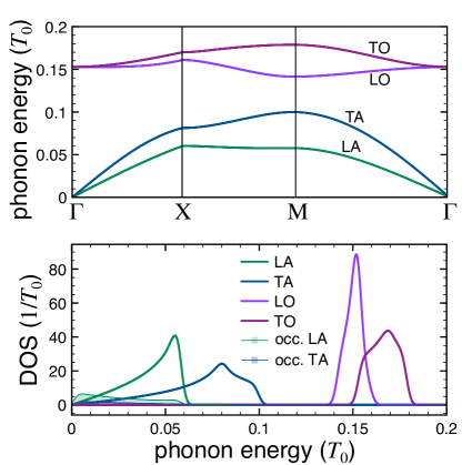
Figure 1: Upper panel: dispersion of the longitudinal acoustic (LA), transverse acoustic (TA), longitudinal optical (LO) and transverse optical (TO) phonon modes. The energy is measured in units of the hopping constant $T_{0}$. Lower panel: corresponding density of states (DOS) along with the occupation-weighted DOS for the LA and TA modes (filled curves).

It should be mentioned that the role of the el-ph coupling in topological insulators, in particular at the surface, is a topic of recent discussions. While some works point out the strong influence of el-ph coupling for inelastic scattering Giraud and Egger (2011); Giraud et al. (2012); Costache et al. (2014) and for intraband relaxation of photoexcited systems Hatch et al. (2011), other measurements suggest weak el-ph interaction effects Pan et al. (2012). Here, we take a different angle and treat the coupling strength $\gamma$ as a parameter.

II.3 Equations of motion in the presence of Electron-phonon interactions

The full Hamiltonian (8) constitutes an interacting electron-boson model. The numerically exact solution is out of reach for the typical number of points in reciprocal space. Furthermore, since the phonon energies $\omega_{\mu}(\mathbf{q})$ are much smaller than the electronic energy scale, a weak-coupling treatment is suitable. In this context, the nonequilibrium Green’s function (NEGF) approach in its time-dependent formulation has become an important tool recently Sentef et al. (2013); Kemper et al. (2013); Murakami et al. (2015); Säkkinen et al. (2015); Murakami et al. (2016); Schüler et al. (2016); Tuovinen et al. (2016). However, most of the approaches resort to a local approximation to the el-ph interaction. This approximation excludes intraband transitions, which are, as discussed above, the only available relaxation channel in our case. Therefore, a momentum-dependent treatment of the phonons is required, which increases the computational costs of the NEGF method considerably. Since neither renormalization effects of the electronic structure due to the coupling to the phonons nor the backaction on the phononic degrees of freedom is of particular significance for the relaxation in the MDM, one can employ a simplified theory based on a master-equation approach within the Markovian approximation Breuer and Petruccione (2002). The usual Lindblad equation, however, is formulated in terms of the many-body density matrix Usenko et al. (2016). For calculating the time evolution of the single-particle density matrix, $\rho_{ij}(\mathbf{k};t)=\langle\hat{c}^{\dagger}_{\mathbf{k}i}(t)\hat{c}_{\mathbf{k}j}(t)\rangle$, additional conditions are required, reflecting not only the overall particle conservation, but the fermionic statistics, as well. This can be achieved by extending the linear Lindblad equation to a nonlinear master equation Rosati et al. (2014, 2015). Alternatively, equivalent master equations can also be obtained from with NEGF formulation within the generalized Kadanoff-Baym ansatz Schlünzen and Bonitz (2016) and applying the Markovian approximation Langreth and Nordlander (1991).

Within the master-equation approach, the equation of motion (EOM) for the single-particle density matrix reads

$$\frac{\mathrm{d}}{\mathrm{d}t}\boldsymbol{\rho}(\mathbf{k};t)=-\mathrm{i}\left[\mathbf{h}_{\mathrm{el}}(\mathbf{k};t),\boldsymbol{\rho}(\mathbf{k};t)\right]+\mathbf{I}(\mathbf{k};t)\ ,$$ (11)

where we have employed a more compact matrix notation. Besides the unitary time evolution captured by the first term, the el-ph coupling is described by the scattering term Rosati et al. (2014)

$$I_{ij}(\mathbf{k};t) =\frac{1}{2}\sum_{\mu\mathbf{q}}\sum_{klm}\Big{[}\bar{\rho}_{ik}(\mathbf{k};t)\mathcal{R}^{\mu\mathbf{q}}_{kl,jm}(\mathbf{k},\mathbf{k}-\mathbf{q})\rho_{lm}(\mathbf{k}-\mathbf{q};t)$$

$$\quad-\bar{\rho}_{kl}(\mathbf{k}+\mathbf{q};t)\mathcal{R}^{\mu\mathbf{q}}_{ki,lm}(\mathbf{k}+\mathbf{q},\mathbf{k})\rho_{mj}(\mathbf{k},t)\Big{]}\ .$$ (12)

Here, $\bar{\rho}_{ij}(\mathbf{k};t)=\delta_{ij}-\rho_{ij}(\mathbf{k};t)$ is the density matrix of the hole states, while $\mathcal{R}^{\mu\mathbf{q}}_{kl,jm}(\mathbf{k}_{1},\mathbf{k}_{2})$ denotes the scattering rate which determines the transition probability. As the scattering events are limited to intraband transitions governed by momentum (and energy) conservation, the scattering rates simplify to Rosati et al. (2015)

$$\mathcal{R}^{\mu\mathbf{q}}_{kl,jm}(\mathbf{k}_{1},\mathbf{k}_{2})=\delta_{\mathbf{k}_{1},\mathbf{k}_{2}+\mathbf{q}}\delta_{kj}\delta_{lm}R^{\mu\mathbf{q}}_{jl}(\mathbf{k}_{1},\mathbf{k}_{2})$$ (13)

with

$$R^{\mu\mathbf{q}}_{jl}(\mathbf{k}_{1},\mathbf{k}_{2})=\frac{\gamma^{2}}{N_{k}}\frac{1}{q^{2}}\left|\mathbf{u}_{\mu\mathbf{q}}\cdot\mathbf{q}\right|^{2}D^{>}_{\mu\mathbf{q}}(\varepsilon_{l}(\mathbf{k}_{2})-\varepsilon_{j}(\mathbf{k}_{1}))\ .$$ (14)

Here, the spectral function of the unoccupied phonon modes (greater Green’s function in the NEGF context) is defined by

$$D^{>}_{\mu\mathbf{q}}(\omega)=2\pi\left(N_{B}(\omega)+1\right)\left[\delta(\omega-\omega_{\mu}(\mathbf{q}))-\delta(\omega+\omega_{\mu}(\mathbf{q}))\right]\ ,$$ (15)

where $N_{B}(\omega)$ denotes the Bose distribution. In practice, the Dirac-$\delta$ functions in Eq. (15) are replaced by Gaussians with a small broadening parameter $\eta$.

Note that the definition of the scattering terms (II.3)–(14) depends on the electronic eigenenergies explicitly. The EOM (11) thus has to be solved in the eigenbasis of $\mathbf{h}_{\mathrm{el}}(\mathbf{k};t=0)$. For the quench scenario, this means the electronic energies in Eq. (14) correspond to the pre-quench Hamiltonian.

The algorithm which we employed for the numerical solution of the master equation (11) is presented in appendix A.

III Observables in equilibrium

Let us now proceed by defining the observables which will be used to trace the nonequilibrium dynamics. We first consider the equilibrium case, where the system is either in the band insulating or QHI phase and then discuss how to extend the schemes to the time-dependent case.

III.1 Circular asymmetry

As suggested by Tran et al. (Ref. Tran et al., 2017), the depletion rate $\Gamma^{(+)}_{n}(\omega)$ ($\Gamma^{(-)}_{n}(\omega)$) upon irradiation of left (right) circularly polarized light with frequency $\omega$ yields a direct measure of the Chern number of band $n$. In particular, the frequency-integrated asymmetry signal $\int\!\mathrm{d}\omega\,(\Gamma^{(+)}_{n}(\omega)-\Gamma^{(-)}_{n}(\omega))$ is proportional to $\mathcal{C}_{n}$. This property was derived for a noninteracting system; however, it is generic and can also be exploited in interacting systems. A closely related effect is the pronounced polarization dependence observed in angle-resolved photoemission (ARPES) from graphene, mapping out the Berry phase of the individual bands Hwang et al. (2011); Liu et al. (2011). Alternative ways of extracting the topological character of the system in experiments is, besides the aforementioned Hall effect, are Aharonov-Bohm-type interferometry Duca et al. (2015) in optical traps and spin-polarized measurements Wu et al. (2016). However, here we focus on observables that can be easily extended to the transient regime.

For the two-band MDM, Fermi’s golden rule yields

$$\Gamma^{(\pm)}_{1}(\omega)\propto\sum_{\mathbf{k}}\left|\langle\phi_{\mathbf{k}2}|\hat{V}^{(\pm)}(\mathbf{k})|\phi_{\mathbf{k}1}\rangle\right|^{2}\delta(\varepsilon_{2}(\mathbf{k})-\varepsilon_{1}(\mathbf{k})-\omega)\ .$$ (16)

Here, the transition operator, derived from the standard Peierls substitution, reads

$$\hat{V}^{(\pm)}(\mathbf{k})=\frac{\partial\hat{h}_{\mathrm{el}}(\mathbf{k})}{\partial k_{x}}\pm\mathrm{i}\frac{\partial\hat{h}_{\mathrm{el}}(\mathbf{k})}{\partial k_{y}}\ .$$ (17)

Provided the transition is permitted by energy conservation, the excitation probability is determined by the matrix elements $D^{(\pm)}(\mathbf{k})=\left|\langle\phi_{\mathbf{k}2}|\hat{V}^{(\pm)}(\mathbf{k})|\phi_{\mathbf{k}1}\rangle\right|^{2}$. The asymmetry $\Delta(\mathbf{k})=D^{(+)}(\mathbf{k})-D^{(-)}(\mathbf{k})$ is presented for the BI and the TI in Fig. 2 (a) and (b), respectively. We neglect the el-ph coupling at this point ($\gamma=0$).

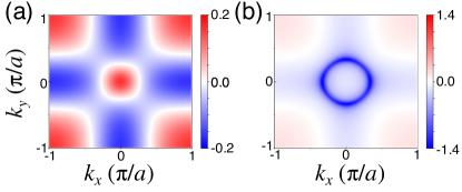
Figure 2: Circular asymmetry $\Delta(\mathbf{k})$ of the transition probability for (a) the BI ($M=M_{\mathrm{BI}}=-5|T_{0}|$) and (b) the TI ($M=M_{\mathrm{TI}}=-3|T_{0}|$) .

As can be seen in Fig. 2, the main difference between BI and TI is the strong negative asymmetry in the vicinity of the $\Gamma$ point in the latter case (panel (b)), which is most pronounced at the $\mathbf{k}$-points where the avoided crossing between the two bands occurs. This can be understood from the fact that $\Delta(\mathbf{k})$ is proportional to the Berry curvature in the two-band case Tran et al. (2017).

In view of transient measurements, it would be most useful to extract the topological character of the system by applying short (circularly polarized) pulses rather than the continuous-wave (plus integrating over frequencies) approach presented in Ref. Tran et al., 2017. Figure 2 suggests to consider transitions close to the $\Gamma$ point, where the difference in the Berry curvature between the BI and TI is most pronounced. The thus required spectral resolution has to be balanced against time resolution determined by the pulse duration. We have chosen electric field pulses of the form

$$\mathbf{E}^{(\pm)}(t)=F_{0}\sin^{2}\left(\frac{\pi(t-t_{0})}{T_{\mathrm{p}}}\right)\mathrm{Re}\big{\{}e^{-\mathrm{i}\omega_{0}(t-t_{0})}\boldsymbol{\epsilon}^{(\pm)}\big{\}}$$ (18)

for $t_{0}<t<t_{0}+T_{\mathrm{p}}$. The left or right polarization vector (superscript $+$ or $-$, respectively) is given by $\boldsymbol{\epsilon}^{(\pm)}=\mathbf{e}_{x}\pm\mathrm{i}\mathbf{e}_{y}$. In order to determine the corresponding asymmetry signal, we propagate the time-dependent Schrödinger equation in the presence of the electric field (18) by the Peierls substitution $\hat{h}^{(\pm)}_{\mathrm{el}}(\mathbf{k};t)\rightarrow\hat{h}^{(\pm)}_{\mathrm{el}}(\mathbf{k}-\mathbf{A}^{(\pm)}(t);t)$ ($\mathbf{A}^{(\pm)}(t)$ is the vector potential corresponding to the field) in the weak-field limit ($F_{0}=0.5$). The expected left-right asymmetry of the depletion rate translates into an asymmetry of the photoexcitation probability. After some tests we found that pulses as short as $T_{\mathrm{p}}=5.0$ offer a good comprise between sharpness in frequency space and pulse duration. The excitation probability for both the BI and the TI case is depicted in Fig. 3 as a function of the central frequency $\omega_{0}$.

Figure 3: Population of the upper band after applying a pulse with central frequency $\omega_{0}$ to the BI (upper panel) and TI (lower panel). The dashed line marks the optimal pulse frequency $\omega_{\mathrm{opt}}$ where the difference between the BI and TI response is most pronounced.

In line with Ref. Tran et al., 2017, integrating over all frequencies yields zero for the BI (since $\mathcal{C}_{1}=0$), while a nonzero value is obtained for the TI. As expected from the behavior of the matrix elements (see Fig. 2), the region in reciprocal space where the Berry curvature is the strongest in the TI case is particularly suited for mapping out the topological character of the system. This leads to the optimal frequency $\omega_{\mathrm{opt}}\simeq 2.5$ where the BI predominantly absorbs left circularly polarized light (corresponding to the red region around the origin in Fig. 2(a)), but where the Berry curvature leads to a strongly enhanced absorption of right circularly polarized radiation in the TI case. Choosing $\omega_{0}=\omega_{\mathrm{opt}}$ we obtain a field pulse which is ideally suited for tracing the transient dynamics of the system upon photoexcitation or after a quench. Note that the absorbance of the BI is reduced compared to the TI due to the larger band gap.

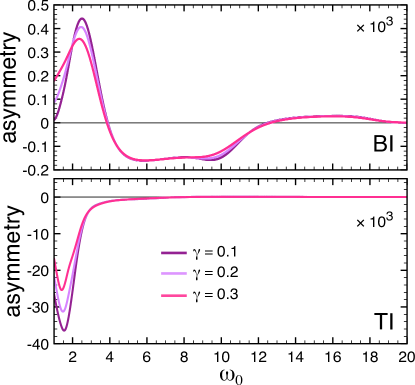
Figure 4: Asymmetry signal analogous to Fig. 3, but for different el-ph coupling strengths $\gamma>0$.

The next important question to address is if a similar behavior can be expected in the presence of el-ph coupling. To address this issue, we solved the master equation (11) including the electromagnetic field and computed, as for the non-interacting case, the photoexcitation probability. The result for several moderate coupling strengths $\gamma$ is presented in Fig. 4. Besides an overall suppression of the absorbance and the less pronounced difference between the the excitation probabilities for left/right circularly polarized light, the qualitative behavior is consistent with the dissipation-less case (Fig. 3). The visible difference of the asymmetry for the relatively strong el-ph couplings demonstrated in Fig. 4 implies that one can obtain valuable information on the topological character even for weak to moderate strength of dissipative effects.

III.2 Time-resolved Hall effect

The emergence of the integer Hall effect $\sigma_{xy}=(e^{2}/h)\mathcal{C}_{1}$ provides direct access to the topological character in equilibrium. A possible extension of this concept to a time-dependent scenario is – similarly as in subsection III.1 – to apply suitably shaped pulses with parameters optimized in the equilibrium case. To this end, we computed the optical conductivity $\sigma_{\alpha\beta}(\omega)$ for both the BI and the TI phase. The real part is shown in Fig. 5.

The plateau in $\sigma_{xy}(\omega)$ at small frequencies gives us some guidance in choosing the spectral features of a suitable probe pulse $\mathbf{E}(t)$ which allows to map out the topological character: (i) the pulse needs to be short to enable us to trace the transient dynamics, (ii) the pulse in frequency space needs to have a maximal overlap with the region $\omega\approx 0$, and (iii) $\int\!\mathrm{d}t\,\mathbf{E}(t)=0$ is required within the dipole approximation. Electromagnetic field pulses which optimally fulfil the criteria (i)–(iii) are half-cycle pulses (HCPs) Moskalenko et al. (2017). HCPs are pulses with a dominant, short peak and a weak and long tail (which hardly influences the dynamics). The dominant peak makes the field effectively unipolar, as the spectral weight is maximal in the vicinity of $\omega\approx 0$. Here we employ the parameterization $\mathbf{E}_{\mathrm{HCP}}(t)=E_{0}\boldsymbol{\epsilon}F_{\mathrm{HCP}}(t-t_{0})$ with

$$F_{\mathrm{HCP}}(t)=x\left(e^{-x^{2}/2}-\frac{1}{b^{2}}e^{-x/b}\right)\ ,\ x=\frac{t}{T_{\mathrm{p}}}\ .$$ (19)

The parameters are the effective pulse duration $T_{\mathrm{p}}$ and the shape parameter $b$, which we fix at $b=8$ in accordance Moskalenko et al. (2006) with typical pulses generated in experiments You et al. (1993); Jones et al. (1993). The analytical expression in Eq. (19) fulfils $\int^{\infty}_{0}\!\mathrm{d}t\,F_{\mathrm{HCP}}(t)=0$ exactly. The corresponding power spectrum in frequency space is shown in Fig. 5. We have found $T_{\mathrm{p}}=10$ to be a good compromise between a short pulse duration and maximal overlap with the plateau region of the TI, as can be seen in Fig. 5.

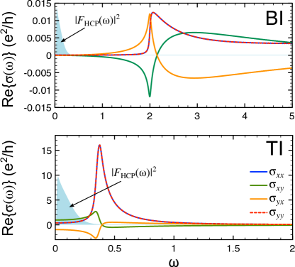
Figure 5: Real part of the optical conductivity for the BI (upper panel) and the TI (lower panel). The filled curve illustrates the power spectrum of the HCP used for the time-dependent calculations (see text). The small but finite value of $\sigma_{xx}(\omega=0)$ is due a small broadening of the Fermi surface.

The properties of the HCPs translate – in combination with the frequency dependence of the optical conductivity – into a distinct behavior of the time-dependent current

$$J_{\alpha}(t)=\sum_{\mathbf{k}}\mathrm{Tr}\left[\mathbf{v}^{\alpha}(\mathbf{k}-\mathbf{A}(t))\boldsymbol{\rho}(\mathbf{k};t)\right]\ .$$ (20)

Here, $\mathbf{v}^{\alpha}(\mathbf{k})=\partial\mathbf{h}_{\mathrm{el}}(\mathbf{k})/\partial k_{\alpha}$ is the velocity matrix. Within the weak-field regime, linear response theory applies and relates the current to the driving field and the optical conductivity:

$$J_{\alpha}(t)=E_{0}\sum_{\beta=x,y}\int^{t}_{0}\!\mathrm{d}t^{\prime}\,\sigma_{\alpha\beta}(t-t^{\prime})\epsilon_{\beta}F_{\mathrm{HCP}}(t^{\prime}-t_{0})\ .$$ (21)

Assuming a linearly polarized HCP in the $x$-direction, the linear response relation (21) yields for the current in the $y$-direction in frequency space

$$J_{y}(\omega)=E_{0}\sigma_{yx}(\omega)F_{\mathrm{HCP}}(\omega)\simeq E_{0}\sigma_{yx}(\omega=0)F_{\mathrm{HCP}}(\omega)\ ,$$ (22)

which implies for the time-dependent current

$$J_{y}(t)\simeq E_{0}\sigma_{yx}(\omega=0)F_{\mathrm{HCP}}(t)\ .$$ (23)

Thus, the current orthogonal to the field polarization is expected to closely resemble the driving pulse in the TI case, while the current will almost vanish for the BI. This behavior is confirmed by the numerical solution of the Schrödinger equation in the presence of the HCP (19) and the resulting time-dependent current $J_{\alpha}(t)$, $\alpha=x,y$ displayed in Fig. 6 for the TI case. The Hall current $J_{y}(t)$ has a strong peak for times where the HCP has its maximum, while the current $J_{x}(t)$ shows an oscillatory behavior. As expected, the simulations show that the Hall current is negligible for the BI phase (not shown).

Figure 6: (a) Time dependent current $J_{\alpha}(t)$ induced by a HCP with $T_{\mathrm{p}}=10$, $t_{0}=10$ and $E_{0}=10^{-4}$, polarized in the $x$-direction. The current has been normalized by the pulse strength. (b) Corresponding pulse-current correlation functions (Eq. (24)) as functions of the delay $\Delta t$.

Since detecting a time-dependent current on the typical time scale of the pulse (which is in the femto- to picosecond range) is difficult in experiments, we propose to analyze the behavior of the pulse-current correlation function

$$C_{\alpha}(\Delta t)=\int^{\infty}_{0}\!\mathrm{d}t\,J_{\alpha}(t)F_{\mathrm{HCP}}(t-\Delta t)\ .$$ (24)

This signal could be detected similarly to the total induced charge, but weighted with the known driving pulse. The behavior of the Hall current $J_{y}(t)$ observed in Fig. 6 can thus be characterized by a peak at $\Delta t=0$, while a transient current response originating from a pronounced variation with respect to the frequency will not possess this feature. This is confirmed in Fig. 6.

IV Tracing the quench dynamics – unitary time evolution

Let us now investigate the dynamics of the system after a quench across the phase boundary and the manifestation of this transition in the observables discussed in subsection III. We focus on the noninteracting case $\gamma=0$ first.

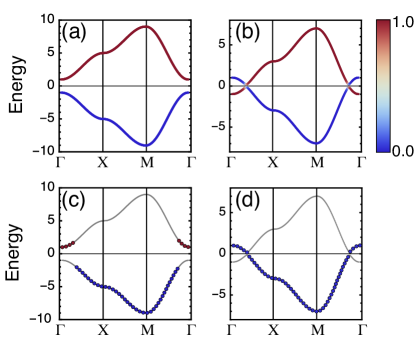
Figure 7: Band structure of (a) the BI and (b) the TI. The coloring of the lines indicates the orbital weight of the upper band underlying the Hamiltonian (1). Band structure of (c) the BI and (d) the TI, where the dots indicate that the occupation of the respective band after the quench is larger than $0.5$. The energy is measure in units of $|T_{0}|$

Assuming that the system is initially in equilibrium ($M=M_{\mathrm{TI/BI}}$) with the lower band completely filled and the upper band empty, the gap parameter is ramped up or down in a time $T_{\mathrm{q}}=5$ (see subsection II.1). This short ramp time corresponds to an almost ideal quench, i. e. the occupations of the post-quench bands is given by

$$f^{\mathrm{B}}_{n}(\mathbf{k})=\left|\langle\phi^{\mathrm{B}}_{\mathbf{k}n}|\psi_{\mathbf{k}1}(t=T_{\mathrm{q}})\rangle\right|^{2}\simeq\left|\langle\phi^{\mathrm{B}}_{\mathbf{k}n}|\phi^{\mathrm{A}}_{\mathbf{k}1}\rangle\right|^{2}.$$ (25)

The post-quench occupation (25) is shown along the standard path in the Brillouin zone of the square lattice in Fig. 7, marked by points where $f^{\mathrm{B}}_{n}(\mathbf{k})>0.5$. In fact, $f^{\mathrm{B}}_{n}(\mathbf{k})$ is close to one for most points.

IV.1 Time-dependent Hall effect

Examining the structure of the density matrix after the quench, one realizes that coherent superpositions of the two bands play a major role, such that the system is far away from a steady state for which the Hall conductance (7) can be defined. However, to have a measure of the post-quench state the system is driven to, we can investigate the response to HCPs as discussed in subsection III.2. The current induced by a HCP polarized along the $x$ direction after performing the quench $M_{\mathrm{BI}}\rightarrow M_{\mathrm{TI}}$ is shown in Fig. 8(a). In comparison to the current response in equilibrium (Fig. 6), the coherent oscillations of the current dominate the hump at times when the electric field of the pulse is strong. The magnitude of these oscillations is considerably larger than in the equilibrium case, showing that the superposition state after the quench is quite different from the equilibrium TI state.

At first glance, is seems that the current in the $y$ direction is not displaying the behavior discussed in subsection III.2, as the magnitude of the current is quite small even when the electric field reaches its maximum. Nevertheless, the pulse-current correlation function $C_{\alpha}(\Delta t)$ defined in Eq. (24) and presented in Fig. 8(b), exhibits the distinct feature of the QHI: $C_{y}(\Delta t)$ possesses a clear maximum at $\Delta t=0$, which indicates a plateau behavior of the optical conductivity $\sigma_{xy}$ at $\omega=0$ and thus the presence of a nonzero Hall effect. The magnitude of $C_{y}(\Delta t=0)$ is, however, significantly (approximately by a factor of four) reduced with respect to the equilibrium case (Fig. 6(b)). Hence one would expect a static Hall conductance of about $\sigma_{xy}\simeq 0.25e^{2}/h$.

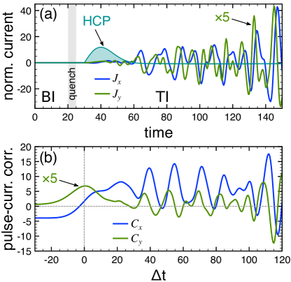
Figure 8: (a) Time-dependent current induced by a HCP (sketched in the plot) after the quench from the BI state to the TI (illustrated by the shaded background). The current in the $y$ direction has been multiplied by $5$ for better visibility. The normalization of the current is consistent with Fig. 6. (b) Corresponding pulse-current correlation functions.

We also performed analogous simulations for the $M_{\mathrm{TI}}\rightarrow M_{\mathrm{BI}}$ quench and found the emergence of a very small, but finite Hall effect after the quench.

The coherent superposition present in the post-quench state results in an internal dynamics which might interfere with transient measurements. However, one can expect decoherence effects to diminish these coherences, leading to a mixed steady state. In this case, the static Hall effect yields valuable information on the post-quench state, as discussed in the next subsection.

IV.2 Steady-state conductance

As can be inferred from Fig. 7, the occupation after the quench reflects the pre-quench situation. For instance, the complete filling of the lower BI band is preserved when switching to the TI, apart from the avoided crossing points. This illustrates the conservation of the topological character of the system as the occupation of bands with the same orbital character (which is interchanged at the crossing points in the TI band structure, see Fig. 7) remains constant. Nevertheless, the Hall effect deviates from the equilibrium behavior, which can be seen by evaluating the steady-state optical conductivity in accordance with Ref. Wang et al., 2016 by

$$\sigma^{\mathrm{B}}_{\alpha\beta}(\omega)=\frac{1}{\omega}\sum_{n}\int\!\!\mathrm{d}\mathbf{k}\,f^{\mathrm{B}}_{n}(\mathbf{k})\int^{\infty}_{0}\!\mathrm{d}t\,e^{i\omega t}\langle\phi^{\mathrm{B}}_{\mathbf{k}n}|\Big{[}\hat{j}_{\mathbf{k}\alpha},\hat{j}_{\mathbf{k}\beta}(t)\Big{]}|\phi^{\mathrm{B}}_{\mathbf{k}n}\rangle\ .$$ (26)

Here, $\hat{j}_{\mathbf{k}\alpha}=\partial\hat{h}^{\mathrm{B}}_{\mathrm{el}}/\partial k_{\alpha}$ denotes the momentum-resolved current operator. The resulting conductivity is shown in Fig. 9. Note that computing the optical conductivity analogously to Eq. (7) assumes that all off-diagonal elements of the density matrix, which capture the coherent oscillations of the system after the excitation, are zero.

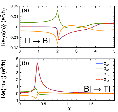
Figure 9: Optical conductivity of the post-quench state $\sigma^{\mathrm{B}}_{\alpha\beta}(\omega)$ according to the definition (26) for (a) the quench $M_{\mathrm{TI}}\rightarrow M_{\mathrm{BI}}$ and (b) $M_{\mathrm{BI}}\rightarrow M_{\mathrm{TI}}$.

As can be inferred from Fig. 9, the Hall conductance significantly deviates from the equilibrium value. In the $M_{\mathrm{TI}}\rightarrow M_{\mathrm{BI}}$ quench, the system acquires a finite Hall conductance $\sigma^{\mathrm{B}}_{xy}(\omega=0)\simeq 0.0038e^{2}/h$, while the quench $M_{\mathrm{TI}}\rightarrow M_{\mathrm{BI}}$ leads to $\sigma^{\mathrm{B}}_{xy}(\omega=0)\simeq 0.25e^{2}/h$. These values are consistent with the time-dependent response discussed in subsection IV.1. Without the unit factor $e^{2}/h$, the latter can be regarded as a nonequilibrium generalization of the Chern number Wang et al. (2016). Note that the concrete numbers depend on both the pre- and the post-quench gap parameter $M$.

IV.3 Transient circular asymmetry

Let us now proceed to transient properties. As discussed in subsection III.1, the circular asymmetry is a very promising candidate for tracing the dynamics in real time. To find a suitable analogue to the equilibrium scenario, we performed test calculations of the population dynamics driven by circularly polarized pulses (with the same parameters as in subsection III.1 and with central frequency $\omega_{0}=\omega_{\mathrm{opt}}$) after the system has been quenched. For the case $M_{\mathrm{BI}}\rightarrow M_{\mathrm{TI}}$ one finds that the system is preferably excited by right circular pulses, while a left circular pulse results in a weaker depletion of the post-quench lower band. In contrast, circularly polarized pulses applied to the BI after the quench from the TI result in a depletion of the upper band instead (irrespective of the polarization). Furthermore, one observes an oscillatory dependence of the photoexcitation probability after a quench, which originates – analogously to the current discussed in subsection IV.1 – from the coherent superposition of the states belonging to the upper and lower band, respectively.

For these reasons, we propose to utilize the absorbed energy $E_{\mathrm{abs}}$ of the left or right circular probe pulses as a footprint of the topological character in nonequilibrium instead. Importantly, the energy absorption can be measured in experiments directly by placing photon detectors behind the sample. It should be noted that $E_{\mathrm{abs}}$ can also be negative when the system is excited, which corresponds to stimulated emission rather than absorption. This difference to the equilibrium case needs to be taken into account. We thus define a transient generalization of the circular asymmetry by

$$\Delta E_{\mathrm{abs}}=\left|E^{(+)}_{\mathrm{abs}}\right|-\left|E^{(-)}_{\mathrm{abs}}\right|$$ (27)

where $E^{(\pm)}_{\mathrm{abs}}$ is the energy of the probe pulse which is absorbed (or emitted) by the system. The time-resolved circular asymmetry signal (27) for both quench scenarios is presented in Fig. 10 as a function of the delay $\Delta t=t_{0}-t_{\mathrm{q}}$ between the starting time of the pulse ($t_{0}$) and the time when the system is quenched ($t_{\mathrm{q}}$). The absorbed energy is computed by taking the energy difference $E^{(\pm)}_{\mathrm{abs}}=E^{(\pm)}_{\mathrm{q+pr}}-E^{(\pm)}_{\mathrm{q}}$, where $E^{(\pm)}_{\mathrm{q}}$ denotes the total energy of the quenched system in absence of the probe pulse, while $E^{(\pm)}_{\mathrm{q+pr}}$ is the total energy of the quenched and probed target. The energy is measured at a sufficiently large reference time after the quench and the pulse.

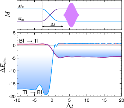
Figure 10: The circular asymmetry of the absorbed energy $\Delta E_{\mathrm{abs}}$ as a function of the delay $\Delta t$ (lower panel) between the quench and the probe pulse (illustrated in the upper panel). The color gradient shading of the curves emphasizes the transition from positive (red) to negative (blue) asymmetry.

Figure 10 demonstrates that the quench dynamics can be traced in the time domain by the circular asymmetry. For the system with $M=M_{\mathrm{BI}}$ before switching, the asymmetry is positive (see Fig. 3). Hence, for $\Delta t<0$ one observes $\Delta E_{\mathrm{abs}}(T_{\mathrm{ref}})>0$ in Fig. 10 for the $M_{\mathrm{BI}}\rightarrow M_{\mathrm{TI}}$ case (purple curve). For $\Delta t>0$, the asymmetry assumes negative values (with larger modulus, as well) which – in accordance to Fig. 3 – indicates the transition to the TI. The opposite behavior can be observed when switching $M_{\mathrm{TI}}\rightarrow M_{\mathrm{BI}}$ (blue curve). Further features are weakly pronounced coherent oscillations of the asymmetry after the quench to the TI which originate from the off-diagonal elements of the time-dependent density matrix. The corresponding time scale is determined by the energy difference between the states whose occupation is changed by the quench.

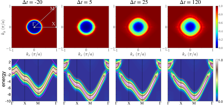
Figure 11: Upper row: time-dependent occupation with respect to the post-quench Hamiltonian (defined by $M=M_{\mathrm{BI}}$) for different time delays $\Delta t$ relative to the quench time (at $\Delta t=0$). Lower row: corresponding tr-ARPES spectra according to Eq. (V.1). The full purple lines indicate the post-quench BI band structure, while the dashed orange lines is the lower band of the TI. The el-ph coupling is set to $\gamma=0.5$.

As our time-dependent simulations demonstrate, the time-resolved quench-probe asymmetry signal based on the absorbed energy provides a robust tool to trace the transient dynamics of the system after a quench. It primarily maps out the circular asymmetry of the underlying bands and is less sensitive to the nonequilibrium occupation. These features clearly distinguish the time-resolved asymmetry from the nonequilibrium Hall effect discussed above and render it a powerful complementary tool.

V Tracing the quench dynamics – dissipative time evolution

After having analyzed the unitary dynamics of the system after a quench, we now investigate how the picture changes if el-ph interactions, as discussed in subsection II.2, are present. Generally, the effect of coupling to the phonon modes is expected to give rise to dissipative dynamics, lowering the energy after the quench excitation. Revisiting Fig. 7 one can expect a qualitatively different behavior for the quench $M_{\mathrm{TI}}\rightarrow M_{\mathrm{BI}}$ as compared to the case $M_{\mathrm{BI}}\rightarrow M_{\mathrm{TI}}$. If the system is quenched from the TI to the BI, the occupation in the upper band (see Fig. 7(a)) is located around the energy minimum at the $\Gamma$ point. Hence, no energy can be extracted from the system after the quench. The effect of the el-ph coupling is in this case primarily the dephasing of the coherences induced by the quench.

V.1 Transient dynamics probed by time-resolved photoemission

We performed numerical simulations of the quench dynamics by solving the master EOM (11) as described in subsection II.3. The parameters are – apart from the el-ph interaction – the same as in section IV. To understand the time evolution of the band structure and the nonequilibrium occupation, the most convenient quantity to look at is the time-dependent occupation with respect to the post-quench basis $f^{\mathrm{B}}_{n}(\mathbf{k};t)=\rho_{nn}(\mathbf{k};t)$ and – as complementary information – the transient photoelectron spectrum. Time-resolved ARPES (tr-ARPES) has recently become a standard tool for tracing the time evolution in correlated systems Schmitt et al. (2008); Graf et al. (2011); Bovensiepen and Kirchmann (2012); Smallwood et al. (2012), in parallel with a rapid development of state-of-the-art theoretical descriptions within the NEGF framework Sentef et al. (2013); Kemper et al. (2013); Murakami et al. (2016). Modeling the photoemission process by a pump pulse (frequency $\omega$, pulse envelope $F_{\mathrm{pr}}(t)$) yields the photocurrent Kemper et al. (2013)

$$I(\mathbf{k};\omega)\propto\mathrm{Im}\int^{\infty}_{-\infty}\!\mathrm{d}t\!\int^{t}_{-\infty}\!\mathrm{d}t^{\prime} \,\left(F_{\mathrm{pr}}(t)\right)^{*}F_{\mathrm{pr}}(t^{\prime})e^{-\mathrm{i}\omega(t-t^{\prime})}$$

$$\times\mathrm{Tr}\left[\mathbf{G}^{<}(\mathbf{k};t,t^{\prime})\right]\ .$$ (28)

Here, $\mathbf{G}^{<}(\mathbf{k};t,t^{\prime})$ denotes the lesser Green’s function, which we express within the generalized Kadanoff-Baym ansatz as $\mathbf{G}^{<}(\mathbf{k};t,t^{\prime})=\mathrm{i}\mathbf{U}(\mathbf{k};t)\boldsymbol{\rho}(\mathbf{k};t^{\prime})$ with the time-evolution operator corresponding to the single-particle Hamiltonian $\mathbf{h}_{\mathrm{el}}(\mathbf{k};t)$. Varying the delay $\Delta t$ between the excitation (the quench at $t_{\mathrm{q}}$ in our case) and the time when the probe pulse is applied, Eq. (V.1) provides a $\mathbf{k}$- and energy-resolved pump-probe spectrum.

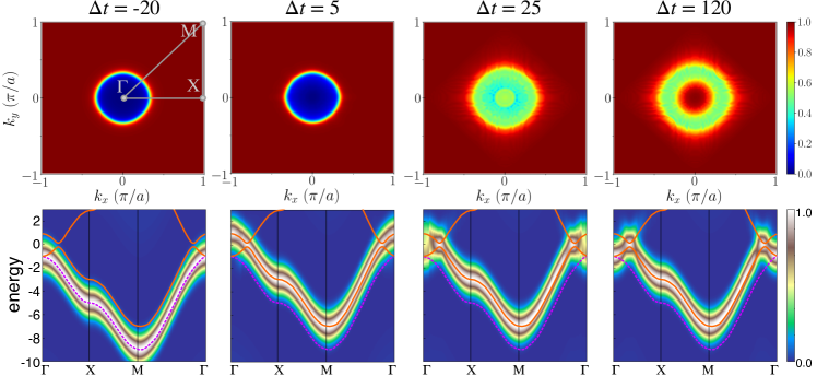
Figure 12: Upper row: time-dependent occupation with respect to the post-quench Hamiltonian (defined by $M=M_{\mathrm{TI}}$) for different time delays $\Delta t$ as in Fig. 11. Lower row: tr-ARPES spectra according to Eq. (V.1). The full purple lines indicate the post-quench TI band structure, while the dashed orange line represents the lower band of the BI. The el-ph coupling is set to $\gamma=0.5$.

In Fig. 11 we present the time-dependent occupation $f^{\mathrm{B}}_{n}(\mathbf{k};t)$ (upper row) along with the corresponding tr-ARPES spectra (lower row) as a function time delay $\Delta t$ for the quench $M_{\mathrm{TI}}\rightarrow M_{\mathrm{BI}}$. In the calculations of the tr-ARPES signals, we used the same parameters for the pulse as in section IV. The short pulse length $T_{\mathrm{p}}=5$ gives rise to the broadening of the spectra in Fig. 11. At $\Delta t=-20$, the system is still in equilibrium and the ARPES signal follows the pre-quench band structure (orange dashed line). The post-quench basis is the BI – therefore, the occupation with respect to the BI bands exhibits a hole around the $\Gamma$ point up to the region where the avoided crossing occurs. This demonstrates a different aspect of the topological state: the occupation of the first Brillouin zone with respect to the dominant orbital character of the lower band is not singly-connected. Following the time evolution right after the quench ($\Delta t=5$) we see a similar picture as in Fig. 7: the ARPES spectrum now follows the post-quench band structure (solid purple lines), while the upper band is populated around the $\Gamma$ point, whereas the lower band is empty in this region. The population assumes values between zero and one around the crossing region, such that a slight lowering of the total energy by el-ph relaxation is possible. This effect can be observed for later times ($\Delta t=25$). The steady state ($\Delta t=120$) however shows only a slight blurring of the occupation compared to directly after the quench.

The nonequilibrium dynamics is considerably more pronounced in the quench scenario $M_{\mathrm{BI}}\rightarrow M_{\mathrm{TI}}$, analyzed again in terms of the time-dependent population of the post-quench lower band in the tr-ARPES spectra in Fig. 12.

Right after the quench ($\Delta t=5$), the ARPES spectrum closely resembles the BI band structure, apart from a shift to larger energies. However, as the occupation of the lower band shows, the post-quench TI band is empty between the $\Gamma$ point and the crossing region, while the upper TI band is populated in this region in the Brillouin zone. It is clear from Fig. 12 that this nonequilibrium occupation does not correspond to an energy minimum as filling the occupation hole in the lower band and a relaxation towards the energy minimum at the crossing points in the upper band result in a lowering of the total electronic energy. These dissipation processes are efficiently mediated by the el-ph interaction as the time-dependent occupation and the ARPES spectra for later times ($\Delta t=25$) demonstrate. The steady state reached at $\Delta t=120$ has a peculiar configuration: the occupation hole around the $\Gamma$ point has been filled, while the population of the upper band has relaxed down to the crossing point. Interestingly, from the ARPES spectrum alone one could suspect that the system has fully relaxed to a TI. However, the nonequilibrium occupation which involves both bands gives rise to a steady-state optical conductivity (Fig. 13) which deviates considerably from the equilibrium behavior (Fig. 5) in its strongly suppressed conductance and Hall conductance. The direct current Hall conductance is reduced to $\sigma_{xy}\simeq 0.003e^{2}/h$ for the quench to the BI, while we find $\sigma_{xy}\simeq 0.05e^{2}/h$ in the $M_{\mathrm{BI}}\rightarrow M_{\mathrm{TI}}$ scenario. Note that the value of the Hall conductance in the TI final state is considerably smaller than in the quench scenario without el-ph interaction (Fig. 9). This can be explained by the distinct occupation in the post-quench steady-state in the presence of the el-ph coupling. The integer Hall conductance $\sigma_{xy}=e^{2}/h$ originates from interband transitions in the crossing region of the upper and lower band. Exactly those transitions are strongly suppressed in the steady-state of Fig. 12, as the occupation in the lower band in the crossing region is depleted, while the available states in the upper band are mostly occupied.

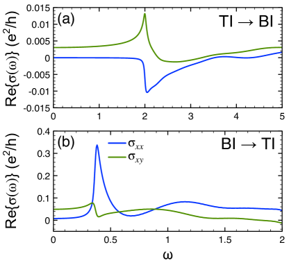
Figure 13: Real part of the nonequilibrium optical conductivity of the post-quench steady-state reached in the presence of el-ph interactions, for (a) the transition $M_{\mathrm{TI}}\rightarrow M_{\mathrm{BI}}$, and (b) the switching $M_{\mathrm{BI}}\rightarrow M_{\mathrm{TI}}$.

V.2 Transient circular asymmetry

Let us now investigate if the transition from the topologically trivial BI to the QHI or vice-versa can be traced in the time domain by circularly polarized pulses in an analogous fashion as for the dissipation-less case discussed in subsection IV.3. We employ the same scheme: a left or right circularly polarized pulse photoexcites the system before, during or after the quench. The energy absorbed by the pulse and, in particular, the left-right asymmetry should then reveal the character of the steady state or transient state. We have applied this recipe, using the definition (27), and present the respective energy absorption asymmetry in Fig. 14 for two representative cases of the el-ph interaction: (i) weak coupling $\gamma=0.1$ (Fig. 14(a)–(b)) and moderate coupling strength $\gamma=0.3$ (Fig. 14(c)–(d)). We represent the absorption asymmetry as a function of the quench-pulse delay $\Delta t$ as in Fig. 10.

For $\gamma=0.1$, Fig. 14(a) shows a transition $M_{\mathrm{BI}}\rightarrow M_{\mathrm{TI}}$ similarly to the unitary case. The asymmetry $\Delta E_{\mathrm{abs}}$ changes from positive values (with small magnitude) to negative, indicating the switch from BI to TI. On the other hand, the quench $M_{\mathrm{TI}}\rightarrow M_{\mathrm{BI}}$ (Fig. 14(b)) is accompanied by a switch of $\Delta E_{\mathrm{abs}}$ from negative to positive values (with strongly reduced magnitude). Generally, the scheme for tracing the quench dynamics works very well for the dissipative case with weak el-ph interaction.

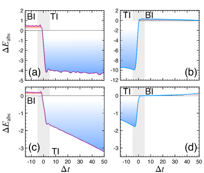
Figure 14: Asymmetry of the absorbed energy $\Delta E_{\mathrm{abs}}$ as a function of the delay $\Delta t$ between the quench and the probe pulse for (a)–(b) weak el-ph coupling $\gamma=0.1$, and (c)–(d) moderate el-ph coupling $\gamma=0.3$. The color gradient filling of the curves is analogous to Fig. 10. The gray shaded area indicates the time when the system is switched from BI to TI (left panels) or TI to BI (right panels), respectively.

Turning to stronger el-ph couplings, the picture slightly changes. For the quench $M_{\mathrm{BI}}\rightarrow M_{\mathrm{TI}}$ (Fig. 14(c)), one can observe the asymmetry $\Delta E_{\mathrm{abs}}$ switching from small positive values to the negative region across the quench. The almost linear decrease of $\Delta E_{\mathrm{abs}}$ towards larger $\Delta t$ is attributed to the el-ph induced relaxation after the pulse (see Fig. 12). One can readily check that the photoexcitation probability due to the specific pulse is larger in the post-quench relaxed steady state than right after the quench, because more states are occupied in the energy window defined by the pulse frequency. Therefore, the absorption of the left-circular probe pulse becomes more efficients as $\Delta t$ increases, until the steady state is reached (at $\Delta t\sim 200$). Generally, the dependence of $\Delta E_{\mathrm{abs}}$ on $\Delta t$ is much more pronounced in the TI phase, since the influence of the el-ph coupling (as discussed in subsection V.1) is stronger.

VI Conclusions

We have studied the quench dynamics of the MDM as a generic model for two-dimensional topological insulators with a special emphasis on how the nonequilibrium and transient properties are reflected in experimentally accessible quantities. We have focused on two promising observables which reveal the topological character of the system: the steady-state and time-dependent Hall effect and the asymmetry of photoexcitation with respect to left or right circularly polarized pulses. Based on a realistic model for two-dimensional topological insulators we have defined suitable probe-pulse shapes by considering the equilibrium model, both for the dissipation-less case and including electron-phonon interactions. We then applied these optimized pulses to trace the nonequilibrium dynamics after a quench. Both the time-dependent Hall effect and the circular dichroism of the absorbed energy provide valuable information on the system. While the Hall current can deliver important insights into the steady state, it turns out to be less suitable for the analysis of transient states. This is due to the coherent superpositions in the system, which give rise to an intrinsic transient dynamics. The circular asymmetry of the absorbed energy, on the other hand, is much less sensitive to these effects, since it is based on the occupation of the bands only. The latter approach is thus particularly well suited for the study of the switching process between different phases.

In the presence of electron-phonon coupling, the quench dynamics can significantly differ from the dissipation-less case, provided the energy of the system is reduced by scattering from phonons. We analyzed these effects in terms of the time-resolved ARPES spectra. We investigated the steady-state properties by the nonequilibrium Hall conductance and, finally, analyzed the quench dynamics in terms of the circular asymmetry. As an important point for the potential experimental realization, we have demonstrated the robustness of our prosed transient measurement in the presence of weak to moderate electron-phonon coupling. The transient circular dichroism has thus been shown as a very promising tool to obtain insights in the up to now little explored field of nontrivial topological phases in nonequilibrium.

Appendix A Numerical solution of the master equation

For a stable numerical solution of a master equation of the type of Eq. (11) we adapt a method for propagating NEGFs in time Stan et al. (2009). The interval $[0,t_{\mathrm{max}}]$ is discretized into an equidistant grid $t_{n}=n\Delta t$. In order to perform the step $\boldsymbol{\rho}(t_{n})\rightarrow\boldsymbol{\rho}(t_{n+1})$, we separate the unitary time evolution from the scattering term by the ansatz

$$\boldsymbol{\rho}(t_{n}+\tau) =\mathbf{U}(t_{n}+\tau,t_{n})\widetilde{\boldsymbol{\rho}}_{n}(\tau)\mathbf{U}^{\dagger}(t_{n}+\tau,t_{n})$$

$$\equiv\mathbf{U}_{n}(\tau)\widetilde{\boldsymbol{\rho}}_{n}(\tau)\mathbf{U}^{\dagger}_{n}(\tau)\ ,\tau\in[0,\Delta t]\ .$$ (29)

Here, $\mathbf{U}(t_{n}+\tau,t_{n})$ denotes the time-evolution operator, which we approximate by $\mathbf{U}_{n}(\tau)\approx\exp[-\mathrm{i}\,\tau\mathbf{h}_{\mathrm{el}}(t_{n}+\Delta t/2)]$. Inserting Eq. (A) into the EOM (11) then yields

$$\boldsymbol{\rho}(t_{n+1}) =\mathbf{U}_{n}(\Delta t)\boldsymbol{\rho}(t_{n})\mathbf{U}^{\dagger}_{n}(\Delta t)$$

$$\quad+\int^{\Delta t}_{0}\!\mathrm{d}\tau\,\mathbf{U}^{\dagger}_{n}(\tau-\Delta t)\mathbf{I}(t_{n}+\tau)\mathbf{U}_{n}(\tau-\Delta t)\ .$$ (30)

Apart from the approximation to the time-evolution operator $\mathbf{U}_{n}(\tau)$, Eq. (A) is still exact. A simple and numerically stable propagation scheme is obtained by approximating $\mathbf{I}(t_{n}+\tau)\approx\mathbf{I}(t_{n}+\Delta t/2)\equiv\mathbf{I}_{n+1/2}$. Using the Baker-Hausdorff formula, the time step (A) can be expressed as

$$\boldsymbol{\rho}(t_{n+1}) =\mathbf{U}_{n}(\Delta t)\boldsymbol{\rho}(t_{n})\mathbf{U}^{\dagger}_{n}(\Delta t)$$

$$\quad+\mathrm{i}\Delta t\sum^{p-1}_{k=0}\frac{(-\mathrm{i}\Delta t)^{k}}{k!}\mathbf{C}^{(k)}_{n}+\mathcal{O}\left((\Delta t)^{p+1}\right)$$ (31)

with $\mathbf{C}^{(0)}_{n}=\mathbf{I}_{n+1/2}$ and $\mathbf{C}^{(k+1)}_{n}=\big{[}\mathbf{h}_{\mathrm{el}}(t_{n}+\Delta t/2),\mathbf{C}^{(k)}_{n}\big{]}$. In practice, we truncate Eq. (A) after the fourth order ($p=4$). The half-step scattering term $\mathbf{I}_{n+1/2}$ is obtained by fourth-order polynomial interpolation using $\mathbf{I}_{n+1-k}$, $k=0,\dots,3$. This requires knowing the scattering term at the next time step, $\mathbf{I}_{n+1}$, which is a function of the yet unknown density matrix $\boldsymbol{\rho}(t_{n+1})$. Therefore, we employ a predictor-corrector scheme where $\mathbf{I}_{n+1/2}$ is first estimated by third-order polynomial extrapolation, allowing to compute $\boldsymbol{\rho}(t_{n+1})$ and thus obtain $\mathbf{I}_{n+1}$. The latter two steps are then iterated at each time step until $\boldsymbol{\rho}(t_{n+1})$ is converged.