Hagedorn Temperature in Superstring Bits and SU(N) Characters

Abstract

We study the simplest superstring bit model at finite $N$ using the characters of the $SU(N)$ group. We obtain exact, analytic expressions for small $N$ partition functions and Gaussian approximations for them in the high temperature limit for all $N$. We use numerical evidence to identify two temperature regimes where the partition function has different limiting behaviors. The temperature at which this transition takes place is identified as the Hagedorn temperature.

I Introduction

The string bit model was first introduced as a microscopic theory of the lightcone quantized relativistic string Giles and Thorn (1977). In this model the string is seen as a polymer of more fundamental units called string bits. To be more specific, each string bit carries an infinitesimal unit of the $+$ component of momentum, $P^{+}=\frac{P^{0}+P^{1}}{\sqrt{2}}$ of the string. As for $P^{-}$, it can be identified as the Hamiltonian of a polymer of string bits. As the number of bits, $M$, becomes large with a fixed $P^{+}$, the excitations of this polymer of bits resemble those of a string with $P^{+}=m\mathcal{M}$, where $m$ is the unit of $P^{+}$ carried by each bit and $\mathcal{M}$ is the bit number operator. These bits are created from the vacuum state $|0\rangle$ by $N\times N$ matrix creation operators, $\bar{\phi}_{\rho}^{\sigma}$, that impose a $U(N)$ color symmetry. Studying the large $N$ expansion Hooft (1974) of the string bit dynamics, then, is equivalent to doing string perturbation theory Thorn (1994). Although initially formulated to describe bosonic strings, this formulation was soon extended to superstrings Bergman and Thorn (1995). The bit creation operator was made completely antisymmetric in an additional set of $p$ “spinor” indices $[u_{1}\cdots u_{p}]$ where $p\in\{0,s\}$ and $u_{q}\in\{1,s\}$ with $s$ denoting the number of Grassmann worldsheet fields in the emergent superstring. Depending upon the number of spinor indices it has, a bit can be either bosonic or fermionic in nature. The superstring bit model that we shall analyze is the simplest possible one: where $s=1$. Recently, it was realized that the matrix creation operator of superstring bits need not be a function of transverse coordinates. Instead it is sufficient to devise another set of two-valued internal “flavor” degrees of freedom, $v_{1}\cdots v_{d}$, where $v_{q}\in\{1,2\}$ with $d$ denoting the number of transverse dimensions Thorn (2014). In this article we work with space-less superstring bits: they have no space dependence. It is important to realize that the string bits do not even have the longitudinal dimension: that arises in the string theory limit. For large $M$, $P^{+}$ becomes effectively a continuous momentum, giving rise to its conjugate: the longitudinal coordinate.

The (canonical) partition function of a system at a thermal equilibrium with a heat bath is defined as

$$Z(\beta)=\int^{\infty}_{0}dE\ g(E)e^{-\beta E}$$ (1)

where $\beta$ is the reciprocal of the product of the Boltzmann constant and the temperature and $g(E)$ is the density of microstates, i.e. the number of states whose energies lie between $E$ and $E+dE$. The partition function can also be regarded as the Laplace transform of the density of states of the system. Also if the density of states increases exponentially with $E$, the partition function can be seen to diverge above a certain temperature (or, equivalently, below a certain value of $\beta$). In statistical mechanics, partition functions can only be singular in the thermodynamic limit. In first order phase transitions, it is the first derivative of the free energy ($\propto\log(Z)$) that is discontinuous. This discontinuity that occurs at the critical temperature, can be attributed to a latent heat in the system. One way to think about a diverging partition function is to imagine an infinite latent heat of the system: it requires adding infinite heat to change the temperature. Phase transitions usually involve liberation of more degrees of freedom in the system under consideration. Hagedorn was studying a thermodynamic model of strongly interacting particles when he found out that for his model to be consistent, the density of states of the system must grow exponentially with energy Hagedorn (1965). This suggested that there is a highest temperature that can be attained by matter (or more specifically, hadrons). Later, dual resonance models were shown to have such exponential dependence of the density of states by Fubini and Veneziano Fubini and Veneziano (1969). This dual resonance model has evolved into what is today known as string theory. In Atick and Witten (1988) the Hagedorn transition is seen as liberating the underlying degrees of freedom in string theory.

This Hagedorn phenomenon was studied in the context of the superstring bit model in Thorn (2015). The superstring bit model used there has $s=1$ and $d=0$. This is the simplest superstring bit model: there are only two kinds of creation operators: $\left(\bar{\phi}\right)_{\rho}^{\sigma}$ and $\left(\bar{\phi}_{1}\right)_{\rho}^{\sigma}$. The former is bosonic (Grassmann-even) and the latter is fermionic (Grassmann-odd) in nature. Since there are only two kinds of bits, we can suppress the spinor indices on the operators, and instead use the symbol ‘a’ for bosonic bits and ‘b’ for fermionic bits. Thus, the only indices that are left are the color indices. The Hamiltonian used in Thorn (2015) can be expressed as

$$H=\frac{T_{0}}{2mN}\text{tr}[(\bar{a}^{2}-i\overline{b}^{2})a^{2}-(\bar{b}^{2}-i\bar{a}^{2})b^{2}+(\bar{a}\bar{b}+\bar{b}\bar{a})ba+(\bar{a}\bar{b}-\bar{b}\bar{a})ba]$$ (2)

where, $T_{0}$ denotes the rest tension of the emergent string, ‘tr’ denotes the trace of the operators over color indices and other symbols denoting the usual quantities we have already defined. The bosonic annihilation operators are defined as $a_{\sigma}^{\rho}=(\bar{a}_{\rho}^{\sigma})^{\dagger}$ and these have the following commutation relation:

$$=\delta_{\sigma}^{\nu}\delta^{\rho}_{\mu}$$ (3)

$\bar{b}_{\rho}^{\sigma}$ have similar definition for annihilation operators, but they follow anti-commutation relation:

$$\{b_{\mu}^{\nu},\bar{b}_{\sigma}^{\rho}\}=\delta_{\sigma}^{\nu}\delta^{\rho}_{\mu}$$ (4)

In this paper we have investigated the onset of the Hagedorn phase transition in our superstring bit model. One important feature of the energy spectrum of string bits under $H$ is that, in the large $N$ limit, the ground state energies of color singlet states and color adjoint states are separated by a finite (and, in the limit $M\rightarrow\infty$, constant) gap. However, the energy scale of string excitations is of $O(1/M)$ Sun and Thorn (2014). One way of interpreting this is that for the singlet states, $H_{\text{eff}}$ is finite and, relatively speaking, for the adjoint states, $H_{\text{eff}}=\infty$. In other words, this interaction gives rise to color confinement: effectively, only the color singlet states are significant in the appropriate limits. This means that instead of using the full Hamiltonian and studying all the states of the system, one may study the Hagedorn phenomenon in a system in which the only dynamics is singlet restriction. This is like imposing color confinement by hand, instead of letting it emerge on its own. As we shall see, this drastically simplified system is still rich enough to support a Hagedorn phenomenon.

The thermal perturbation scheme developed in Thorn (2015) is well defined for arbitrary large values of temperature, and yet the density of singlet states at large $N$ Chen and Sun (2016) suggest a finite limiting temperature. This suggests that the Hagedorn phenomenon is an artifact of the large $N$ limit. In this paper we study the superstring bit model at finite $N$ with $H=0$ and singlet restrictions in order to understand the source of the Hagedorn phenomenon at $N\rightarrow\infty$. We present some exact results for low $N$ partition functions and approximations in the high temperature limit. We also obtain numerical data and analyze them to identify and establish the difference in the behavior of superstring bits below and above the Hagedorn temperature.

II Counting of singlets at large N

Let us set up the problem that we are studying in this paper. We have already described the model that we are studying. We have also explained that we are using $H=0$ and restricting ourselves to the singlet sector. As we are studying the thermal properties of the system, we shall be working with the canonical partition function for a system of superstring bits. In terms of light-cone parameters,

$$P^{-} =H=0$$

$$\implies P^{0} =\frac{P^{+}+P^{-}}{\sqrt{2}}$$

$$=\underbrace{\frac{m}{\sqrt{2}}}_{=\ \omega}\mathcal{M}=\omega\ \text{tr}(\bar{a}a+\bar{b}b)$$ (5)

Our partition function would then be defined as $Z=\text{Tr}\exp(-\beta P^{0})$ where ‘Tr’ denotes the thermal trace, i.e. the trace over all the singlet eigenstates. Since, $H\propto T_{0}$ (Eq. 2), the $H=0$ limit can also be regarded as the tensionless limit of the emergent string.

II.1 Only bosonic bits

Let us derive the large $N$ partition function when there is only one bosonic oscillator. For this, a basis element for color singlets can be written, up to a normalization constant, as:

$$|\text{singlet}\rangle_{\text{bos}}=\text{tr}(\bar{a})^{l_{1}}\text{tr}(\bar{a}^{2})^{l_{2}}\cdots|0\rangle=\left(\prod_{r=1}^{\infty}\text{tr}(\bar{a}^{r})^{l_{r}}\right)|0\rangle$$

where each $l$ can be any non-negative integer. In fact, there is a one-to-one correspondence between the set of all such singlets and the set of sequences ($l_{1},l_{2},\cdots$). Then, energy of such a state is given by:

$$P^{0}|\{l_{r}\}\rangle_{\text{bos}} =\omega\left(\sum_{r=1}^{\infty}rl_{r}\right)|\{l_{r}\}\rangle_{\text{bos}}$$

$$\implies e^{-\beta P^{0}}|\{l_{r}\}\rangle_{\text{bos}} =\left(\prod_{r=1}^{\infty}e^{-\beta\omega rl_{r}}\right)|\{l_{r}\}\rangle_{\text{bos}}$$ (6)

where $\omega$ is defined as in Eq. 5. In the large $N$ limit all these states form an orthogonal eigenbasis of the system. Hence, in that limit, the singlet partition function for pure bosons is:

$$\lim_{N\rightarrow\infty}Z_{\text{bos}}(\beta)=\sum_{\{l_{1},l_{2},\cdots\}}\prod_{r=1}^{\infty}e^{-\beta\omega rl_{r}}=\prod_{r=1}^{\infty}\frac{1}{1-e^{-\beta\omega r}}$$ (7)

II.2 Only fermionic bits

For one fermionic oscillator, one has to be careful, because some of the single trace operators are simply zero. This is because of the cyclic property of the matrix trace and the anti-commutativity of the $\bar{b}$s. E.g.

$$\text{tr}(\bar{b}^{2})=-\text{tr}(\bar{b}^{2})=0$$

In fact, all trace operators with an even number of bits are zero. Hence, a basis element for fermion singlets looks like

$$|\text{singlet}\rangle_{\text{fer}}=\text{tr}(\bar{b})^{k_{1}}\text{tr}(\bar{b}^{3})^{k_{3}}\cdots|0\rangle=\left(\prod_{r=1}^{\infty}\text{tr}(\bar{b}^{2r-1})^{k_{2r-1}}\right)|0\rangle$$

where, each $k$ can take only two values: $0$ and $1$. Hence, for the large-$N$ partition function, we have:

$$\lim_{N\rightarrow\infty}Z_{\text{fer}}(\beta)=\sum_{\{k_{1},k_{3},\cdots\}=0}^{1}\ \prod_{r=1}^{\infty}e^{-\beta\omega(2r-1)k_{2r-1}}=\prod_{r=1}^{\infty}\{1+e^{-\beta\omega(2r-1)}\}$$ (8)

II.3 Supersymmetric case

One may verify that neither $Z_{\text{bos}}$ nor $Z_{\text{fer}}$ diverges at a finite temperature. However, in the supersymmetric case, it can be shown that there is an exponential degeneracy in the number of singlets Chen and Sun (2016), and thereby a finite Hagedorn temperature. Naively, this can be understood as follows: each bit can be either bosonic or fermionic, hence there are roughly $2^{M}/M$ possibilities for a single trace operator of $M$ supersymmetric bits (multi trace states are singlets as well). Of course, some of these combinations don’t correspond to physical states because of the arrangement of anti-commuting fermionic operators in them. E.g.

$$\text{tr}(\bar{b}\bar{a}^{2}\bar{b}\bar{a}^{2})=\text{tr}(\bar{b}\bar{b}\bar{a}^{2}\bar{a}^{2})=-\text{tr}(\bar{b}\bar{a}^{2}\bar{b}\bar{a}^{2})=0$$

However, in the large $M$ limit, this doesn’t harm the exponential degeneracy of eigenstates. In fact, the degeneracy of single trace states goes as $2^{M-1}/M$ for large $M$ Chen and Sun (2016); Aharony et al. (2004); Sundborg (2000). One may calculate an approximation to the partition function starting from this degeneracy. It turns out that the exact supersymmetric partition function,

$$\lim_{N\rightarrow\infty}Z(\beta)=\prod_{n=1}^{\infty}{\frac{1}{1-2\ \exp\{-\beta\omega(2n-1)\}}}$$ (9)

A complete derivation of the generalized result and some interesting sub-cases will appear in Curtright et al. (2017). As is evident from Eq. 9, $Z$ diverges at $\exp\{-\beta\omega\}=1/2$ (it also diverges at other, larger values of temperature). Hence, as anticipated, the supersymmetric case has a Hagedorn temperature at $T_{H}=\omega/\log(2)$. We shall come back to this result in section V.

All the results quoted in this section are applicable in the large $N$ limit. In this paper we wish to study finite $N$ partition functions. Hence, we have to develop a systematic method of counting the eigenstates (i.e. singlets that are linearly independent) for this model at finite $N$. This is what we shall do in the next section.

III From characters to partition functions

Imposing the singlet restriction on the Fock space of all physical states is a purely group theoretic exercise. In our case, the group under consideration is $SU(N)$, the gauge group of the model. A bit creation operator has two color indices and transforms under the adjoint action of $SU(N)$. Given a number of such adjoint operators we shall count the number of ways in which one may obtain states that transform trivially under $SU(N)$. This is very similar to decomposing a direct product of representations into a direct sum of irreps.

Before proceeding with the supersymmetric case, let us examine the pure bosonic and pure fermionic cases at finite $N$. The partition functions are

$$Z_{\text{bos}}(N,\beta) =\prod_{r=1}^{N}\frac{1}{1-e^{-\beta\omega r}}$$ (10)

$$Z_{\text{fer}}(N,\beta) =\prod_{r=1}^{N}\{1+e^{-\beta\omega(2r-1)}\}$$ (11)

As one can see, these expressions are similar to $N\rightarrow\infty$ ones, except that the product over $r$ has been truncated at $r=N$. This is because when $N$ is finite, for $L>N$, $\bar{a}^{L}$ is linearly dependent on $\bar{a}^{c}$s for $c\in\{1,2,\cdots,N\}$. One can obtain the exact dependence from the Cayley-Hamilton theorem, which also gives trace identities for different powers of any square matrix over a commutative ring. For the fermionic case, one has to use a generalized version of the Cayley-Hamilton theorem in order to obtain the cutoff. However, there is another explanation for the fermionic result: it is the Poincaré polynomial for $SU(N)$ (see, for example, ch VII sec 11 of Weyl (1946)). The coefficients of powers of $e^{-\beta\omega}$ in this polynomial count the number of invariants that are linear but completely antisymmetric in the infinitesimal elements of $SU(N)$.

Now that we have stated the special cases, let us focus on the task at hand. For this purpose, we shall use group characters. We shall make use of the orthogonality of characters of different irreps of a group. More specifically, the idea is to obtain the representational content of a physical state by writing down its character. Given this character, one may extract the multiplicity of an irrep within it by taking its product with the conjugate of the character of the said irrep, integrating this over the entire group and then normalizing the integral:

$$g_{RR^{\prime}}=\frac{\int_{G}\{\prod_{i}d\theta_{i}\}\ h(\{\theta_{i}\})\ \chi^{\ast}_{R}(\{\theta_{i}\})\ \chi_{R^{\prime}}(\{\theta_{i}\})}{\int_{G}\{\prod_{i}d\theta_{i}\}\ h(\{\theta_{i}\})}$$ (12)

where $g_{RR^{\prime}}$ denotes the multiplicity of the irrep $R$ in the reducible representation $R^{\prime}$, $h(\{\theta_{i}\})$ denotes the Haar measure on the group G and $\chi_{R}(\{\theta_{i}\})$ represents the character of the representation $R$. All these quantities are parametrized in terms of {$\theta_{i}$}; the rotation angles corresponding to the Cartan subalgebra of the group G. This is very much like using a projection operator to extract out the subspace of irrep $R$. Instead of the character for only one state, one can use a suitable character generating function and obtain the corresponding multiplicity generating function. In Curtright and Thorn (1986) such a generating function was derived to obtain multiplicities at arbitrary mass levels of strings.

For $SU(N)$, the Haar measure is given by

$$\prod_{1\leqslant i<j\leqslant N}|e^{i\theta_{j}}-e^{i\theta_{i}}|^{2}=\prod_{1\leqslant i<j\leqslant N}4\sin^{2}\left(\frac{\theta_{i}-\theta_{j}}{2}\right)$$ (13)

Also, the character for a singlet, the irrep we seek, is simply $1$. Let us figure out how to write down the character for a given state. As mentioned earlier, a creation operator, $\bar{a}^{\mu}_{\nu}$ or $\bar{b}^{\mu}_{\nu}$, transforms in the adjoint representation of $SU(N)$. As such, its upper and lower indices can be regarded as transforming in the fundamental and the anti-fundamental representations, respectively. The character of an operator transforming in the fundamental (anti-fundamental) representation is just $\exp\{i\theta_{k}\}$ ($\exp\{-i\theta_{k}\}$) where $\theta_{k}$ is the rotation angle corresponding to it. Hence, the character for a state $\bar{a}_{\nu}^{\mu}|0\rangle$ or $\bar{b}_{\nu}^{\mu}|0\rangle$ is given by $\exp\{i(\theta_{\mu}-\theta_{\nu})\}$. In doing this exercise, we have made an oversimplification: the adjoint irrep isn’t strictly the direct product of the fundamental and the anti-fundamental irreps. We shall compensate for this error in a moment.

Given a pair of color indices, ($i,j$), an arbitrary multiplet can be represented as

$$\left(\bar{a}^{i}_{j}\right)^{l_{ij}}\left(\bar{b}^{i}_{j}\right)^{k_{ij}}|0\rangle$$

where $l_{ij}$ can be any non-negative integer and $k_{ij}$ can be either $0$ or $1$. From this, one may construct a character generating function for the all states with colors ($i,j$):

$$\frac{1+xe^{i(\theta_{i}-\theta_{j})}}{1-xe^{i(\theta_{i}-\theta_{j})}}=\left(1+xe^{i(\theta_{i}-\theta_{j})}\right)\left(1+xe^{i(\theta_{i}-\theta_{j})}+x^{2}e^{2i(\theta_{i}-\theta_{j})}+\cdots\right)$$ (14)

The numerator above counts the contribution from the fermionic bits while the denominator refers to the contributions coming from the bosonic bits. Hence, the character generating function of any multiplet of any number of superstring bits is given by the expression

$$\prod_{1\leqslant i,j\leqslant N}\frac{1+xe^{i(\theta_{i}-\theta_{j})}}{1-xe^{i(\theta_{i}-\theta_{j})}}=\left(\frac{1+x}{1-x}\right)^{N}\prod_{1\leqslant i<j\leqslant N}\frac{1+x^{2}+2x\cos(\theta_{i}-\theta_{j})}{1+x^{2}-2x\cos(\theta_{i}-\theta_{j})}$$ (15)

So far in this derivation we have approximated the adjoint irrep as a direct product of fundamental and anti-fundamental irreps. However, this product includes an additional irrep: the $U(1)$ singlet. Eq. 15, technically speaking, gives the $U(N)$ character of our model. In order to obtain the generating function for $SU(N)$ we have to remove the tr$(\bar{a})$ from each $\bar{a}_{\nu}^{\mu}$ and tr$(\bar{b})$ from each $\bar{b}_{\nu}^{\mu}$.

$$\left(\frac{1+x}{1-x}\right)^{N-1}\prod_{1\leqslant i<j\leqslant N}\frac{1+x^{2}+2x\cos(\theta_{i}-\theta_{j})}{1+x^{2}-2x\cos(\theta_{i}-\theta_{j})}$$

The coefficient of $x^{M}$ in the expression above gives the correct $SU(N)$ character of the subspace of states with bit number $M$. If we cast this character generating function into Eq. 12 we obtain the generating function for multiplicities of singlet states

$$\sum_{M=0}^{\infty}{{g_{M}}\ x^{M}}=\left(\frac{1+x}{1-x}\right)^{N-1}\frac{\int^{\pi}_{-\pi}\left(\prod^{N}_{k=1}d\theta_{k}\right)\prod_{1\leqslant i<j\leqslant N}4\sin^{2}\left(\frac{\theta_{i}-\theta_{j}}{2}\right)\frac{1+x^{2}+2x\cos(\theta_{i}-\theta_{j})}{1+x^{2}-2x\cos(\theta_{i}-\theta_{j})}}{\int_{-\pi}^{\pi}\left(\prod^{N}_{k=1}d\theta_{k}\right)\prod_{1\leqslant i<j\leqslant N}4\sin^{2}\left(\frac{\theta_{i}-\theta_{j}}{2}\right)}$$ (16)

The R.H.S. of this equation has the following properties:-

1. The integrand in the denominator is the $x\rightarrow 0$ (low temperature) limit of the integrand in the numerator. It can also be interpreted as the “volume” of the $SU(N)$ group and evaluates to $N!(2\pi)^{N}$.

2. The integrand is completely symmetric in the {$\theta_{k}$}s.

3. It is also periodic in each $\theta_{k}$. Hence, the domain of integration is $\mathbb{T}^{N}$, i.e. the $N$-torus.

4. The integrand is a function of differences of $\theta_{k}$’s; in fact it includes all the ${}^{N}C_{2}$ differences among the $\theta_{k}$ ’s. This tells us that the integral is translation-invariant in the $\theta_{k}$’s.

5. The integrand (or rather, the Haar measure) vanishes if $\theta_{i}=\theta_{j}$ for any $i\neq j$.

This generating function gives the multiplicities of singlets at any bit number. In our model, $E=\omega M$ since, $H=0$. If we identify $x$ in this function with $\exp\{-\beta\omega\}$, the L.H.S. of Eq. 16 becomes the (canonical) partition function.

$$\sum_{M=0}^{\infty}{g_{M}\ \exp\{-\beta\omega M\}}=Z(N,\beta)$$

Thus, all partition functions mentioned so far (Eqs. 7, 8, 9, 10, 11), are just different generating functions of $U(N)$ characters. In order to obtain the corresponding $SU(N)$ characters, one must multiply them with $\frac{1-x}{1+x}$. From here onwards, whenever we mention partition functions we shall be referring to generating functions of $SU(N)$ characters. Also for simplicity, we shall express $Z$ as a function of $x(=\beta\omega)$ as opposed to $\beta$.

IV High Temperature Limit of Z

The partition functions for some values of $N$ have been tabulated in TAB. 1 and plotted in FIG. 1. Beyond $N=2$, the character integral becomes too involved to be done analytically by hand. We used a computer to obtain results for $N>2$. Beyond $N=3$, it is useful to employ a change of variables $e^{i\theta_{j}}\rightarrow z_{j}$, in order to turn this integration problem into a problem of calculating (multidimensional) residues:

$$Z(N,x)=\frac{1}{N!}\left(\frac{1+x}{1-x}\right)^{N-1}\sum_{\mathbb{T}^{N}}\text{Res}\left(\prod_{1\leqslant i<j\leqslant N}\frac{-(z_{i}-z_{j})^{2}(xz_{i}+z_{j})(xz_{j}+z_{i})}{(xz_{i}-z_{j})(xz_{j}-z_{i})}\prod_{1\leqslant k\leqslant N}\frac{1}{(z_{k})^{N}}\right)$$ (17)

However, even calculating these residues is prohibitively time-consuming for $N>6$.

$N$	$Z(x)$
2	$(1-x+2x^{2})/(1-x)$
3	$(1+x)(1-2x+4x^{2}-3x^{3}+4x^{4}+2x^{5}+4x^{7})/\left[(1-x)^{2}(1+x+x^{2})\right]$
4	$(1+x)(1-3x+6x^{2}-7x^{3}+9x^{4}-6x^{5}+10x^{6}-2x^{7}+12x^{8}+8x^{9}+8x^{10}+16x^{11}+8x^{12}+8x^{13}+8x^{14})/\left[(1-x)^{3}(1+x+x^{2})\right]$
5	$(1+x)^{2}(1-4x+10x^{2}-17x^{3}+26x^{4}-31x^{5}+40x^{6}-36x^{7}+49x^{8}-18x^{9}+42x^{10}+52x^{11}+38x^{12}+148x^{13}+108x^{14}+240x^{15}+244x^{16}+344x^{17}+376x^{18}+392x^{19}+448x^{20}+352x^{21}+360x^{22}+272x^{23}+176x^{24}+144x^{25}+64x^{26}+32x^{27}+16x^{28})/\left[(1-x)^{4}(1+x+x^{2})(1+x+x^{2}+x^{3}+x^{4})\right]$
6	$(1+x)^{2}(1-4x+10x^{2}-18x^{3}+30x^{4}-41x^{5}+59x^{6}-68x^{7}+98x^{8}-84x^{9}+140x^{10}-41x^{11}+206x^{12}+128x^{13}+442x^{14}+572x^{15}+1130x^{16}+1764x^{17}+2824x^{18}+4468x^{19}+6616x^{20}+9712x^{21}+13688x^{22}+18656x^{23}+24488x^{24}+31152x^{25}+38016x^{26}+44632x^{27}+50640x^{28}+54792x^{29}+57120x^{30}+57056x^{31}+54368x^{32}+49632x^{33}+43232x^{34}+35776x^{35}+28160x^{36}+21088x^{37}+14816x^{38}+9824x^{39}+6144x^{40}+3488x^{41}+1856x^{42}+896x^{43}+352x^{44}+128x^{45}+32x^{46})/\left[(1-x)^{5}(1+x+x^{2})^{2}(1+x+x^{2}+x^{3}+x^{4})\right]$
$\vdots$	$\vdots$
$\infty$	$(1-x)/\left[(1+x)\ \prod_{k=1}^{\infty}(1-2x^{2k-1})\right]$

Table 1: Partition functions that are known exactly.

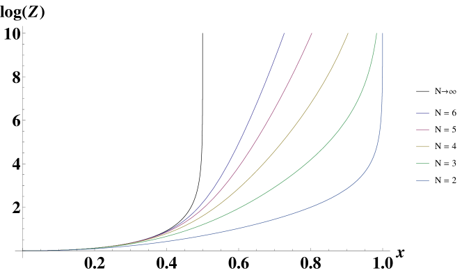
Figure 1: Temperature dependence of known partition functions

We have already identified the $x\rightarrow 0$ limit of Eq. 16 : it is when the R.H.S. becomes $1$ as the numerator becomes equal to the denominator. Let us now concentrate on the $x\rightarrow 1$ (high temperature) limit.

$$Z(N,x\rightarrow 1)=\left(\frac{2}{1-x}\right)^{N-1}\frac{\int^{\pi}_{-\pi}\prod^{N}_{k=1}d\theta_{k}\prod_{1\leqslant i<j\leqslant N}4\cos^{2}\left(\frac{\theta_{i}-\theta_{j}}{2}\right)}{N!(2\pi)^{N}}$$ (18)

As before, evaluating this integral analytically isn’t straightforward beyond the first few values of $N$. The results for $N=2-5$ can be trivially obtained. Beyond $N=5$, one has to use the corresponding multidimensional residue form

$$\left(\frac{2}{1-x}\right)^{N-1}\frac{R_{N}}{N!}$$

where

$$R_{N}=\text{Res}\left(\frac{\prod_{1\leqslant i<j\leqslant N}(z_{i}+z_{j})^{2}}{\prod_{1\leqslant k\leqslant N}(z_{k})^{N}}\right)$$ (19)

This has only one pole (of order $N$) enclosed in the domain of integration; it is at the origin, $(0,\cdots,0)$. For evaluating $R_{N}$, it can also be interpreted as the coefficient of the term $\prod_{1\leqslant k\leqslant N}\ (z_{k})^{N-1}$ in the Taylor-series expansion of $\prod_{1\leqslant i<j\leqslant N}\ (z_{i}+z_{j})^{2}$ about the origin of the $\mathbb{T}^{N}$. This term has every $z_{k}$ raised to the same power ($N-1$), consequently, its coefficient is the biggest of all the coefficients in the Taylor series. Here too, beyond $N>7$ the computation becomes increasingly time-consuming. A list of the calculated $R_{N}$ values can be found in TAB. 2.

N	$R_{N}$
2	2
3	10
4	152
5	7736
6	1375952
7	877901648

Table 2: Exact values of $R_{N}$.

Asymptotic Behavior: Steepest Descent

Since, we don’t have a closed form expression for different coefficients of $\prod_{1\leqslant i<j\leqslant N}\ (z_{i}+z_{j})^{2}$, we turned to its asymptotic analysis. Examining the expression $R_{N}$ we see that it is clearly greater than $2^{N(N-1)/2}$, as the latter is the coefficient of the term $\prod_{1\leqslant k\leqslant N}(z_{k})^{N-1}$ in the Taylor series of $\prod_{1\leqslant i<j\leqslant N}2z_{i}z_{j}$. Similarly, $4^{N(N-1)/2}=2^{N(N-1)}$ is a conservative upper bound on $R_{N}$, as it is the sum of all coefficients in the expansion of the $\prod_{1\leqslant i<j\leqslant N}(z_{i}+z_{j})^{2}$. With these two bounds we can deduce the $N$ dependence of $R_{N}$: it goes as $\exp(N^{2})$ in the leading order. This is an important feature and we shall refer to this observation later. Examining Eq. 18, we see that the integrand attains its maximum value when all the $\theta$s are equal to each other. If one fixes the value of, say $\theta_{1}$, to be $\psi$; the modified integrand attains a single, isolated global maximum at $\theta_{2}=\theta_{3}=\cdots=\theta_{N}=\psi$. While this modification doesn’t change the value integral (or $R_{N}$), but it allows for a simpler, more accurate way of approximating it: by the method of steepest descent.

The method of steepest descent is well known for approximating integrations with a fixed number of dimensions. In our case, however, the number of dimensions isn’t fixed, it’s increasing. In fact, $N$ itself is the large parameter in our case. This isn’t obvious as integrand has an implicit dependence on $N$.

Let us express the general integrand in Eq. 16 as $\exp\left\{\widehat{f}(x,\{\theta_{k}\})\right\}$, where

$$\widehat{f}(x,\{\theta_{k}\})=\sum_{1\leqslant i<j\leqslant N}\log\left\{4\sin^{2}\left(\frac{\theta_{i}-\theta_{j}}{2}\right)\frac{1+x^{2}+2x\cos(\theta_{i}-\theta_{j})}{1+x^{2}-2x\cos(\theta_{i}-\theta_{j})}\right\}$$ (20)

For large $N$, one can convert this restricted double sum into the Cauchy principle value of a double integral. We introduce an integration variable $y_{i}$ such that $y_{i}=\frac{i}{N}\implies dy_{i}=\frac{\Delta i}{N}=\frac{1}{N}$ and a non-decreasing function $\Theta(y)$ for $y\in(0,1]$ such that $\Theta(y_{i})=\theta_{i}$. While defining $\Theta$ we have taken advantage of the fact that in $\widehat{f}(x,\{\theta_{k}\})$, the order of the sequence of $\theta$s doesn’t matter. Hence, one can always redefine the $\theta$s such that they form a non-decreasing sequence, thereby allowing us to define a unique function in the continuum limit. Now, $\widehat{f}(x,\{\theta_{k}\})$ can re-written as

$$\widehat{f}(x,\{\theta_{k}\})=\widehat{f}(N,x)=N^{2}\lim_{\epsilon\rightarrow 0}\int_{0}^{1}\int_{0}^{y-\epsilon}\log\left\{4\sin^{2}\left(\frac{\Theta(y^{\prime})-\Theta(y)}{2}\right)\frac{1+x^{2}+2x\cos(\Theta(y^{\prime})-\Theta(y))}{1+x^{2}-2x\cos(\Theta(y^{\prime})-\Theta(y))}\right\}dy^{\prime}dy$$ (21)

As can be seen above, going to the continuum limit brings out an overall factor of $N^{2}$, thereby making the dependence of $\widehat{f}(x,\{\theta_{k}\})$ on $N$ explicit. Now that we have justified applying the method of steepest descent to our problem, we can see what it yields in the high temperature limit. It gives

$$R_{N}=\frac{2^{N(N-1)}}{\pi^{(N-1)/2}N^{N/2-1}}$$ (22)

which is a more stringent upper bound than $2^{N(N-1)}$. A detailed derivation of this result may be found in the appendix. All these approximations have been plotted against known exact values in FIG. 2.

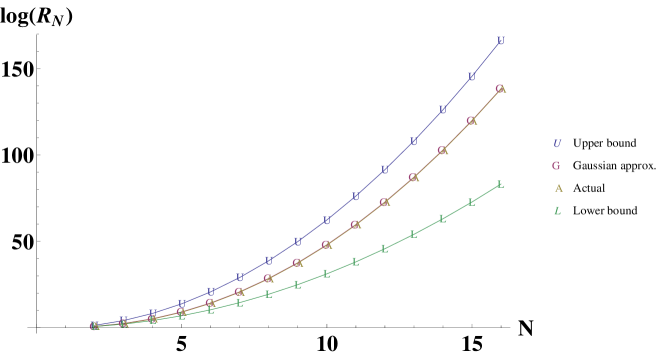
Figure 2: Different estimates of $R_{N}$ at infinite temperature. The exact values for $N>7$ were obtained from McKay (1983)

Another useful way of expressing $\widehat{f}(N,x)$ is:

$$\widehat{f}(N,x)=N^{2}\lim_{\delta\rightarrow 0}\int_{0}^{2\pi}\int_{0}^{\Theta-\delta}\log\left\{4\sin^{2}\left(\frac{\Theta^{\prime}-\Theta}{2}\right)\frac{1+x^{2}+2x\cos(\Theta^{\prime}-\Theta)}{1+x^{2}-2x\cos(\Theta^{\prime}-\Theta)}\right\}\rho(\Theta^{\prime})\ d\Theta^{\prime}\rho(\Theta)\ d\Theta$$ (23)

where we have introduced a normalized density function, $\rho(\Theta)$ such that $dy=\rho(\Theta)\ d\Theta$ and $\int_{0}^{2\pi}{\rho(\Theta)\ d\Theta}=1$. Now, the global maxima of $\widehat{f}(x,\{\theta_{k}\})$ contribute most to the Gaussian approximation. Hence, the density function of the global maxima are of particular interest while doing the integral. The stationarity condition for $\widehat{f}(x,\{\theta_{k}\})$, for $k\in\{1,2,\cdots,N\}$:

$$\sum_{l\neq k}{\cot\left(\frac{\theta_{k}-\theta_{l}}{2}\right)-\frac{4x(1+x^{2})\sin(\theta_{k}-\theta_{l})}{1+x^{4}-2x^{2}\cos\{2(\theta_{k}-\theta_{l})\}}}=0$$ (24)

If $\{\psi_{k}\}$ is a global maximum, then the density function, $\rho(\Psi)$ must be a solution of:

$$\fint_{-\Psi_{[\text{max}]}}^{\Psi_{[\text{max}]}}{\left\{\cot\left(\frac{\Psi^{\prime}-\Psi}{2}\right)-\frac{4x(1+x^{2})\sin(\Psi^{\prime}-\Psi)}{1+x^{4}-2x^{2}\cos\{2(\Psi^{\prime}-\Psi)\}}\right\}\rho(\Psi)\ d\Psi}=0$$ (25)

where $\fint$ denotes the principal value of the integral and the limits are such that $\rho\left(\pm\Psi_{[\text{max}]}\right)=0$ and $\Psi_{[\text{max}]}\leqslant\pi$. This technique follows from Brézin et al. (1978) where the authors study the Hermitian matrix model. They used this technique to obtain an analytic expression for the density function of the eigenvalues in the presence of quartic and cubic interactions. We shall come back to these density functions later in the article.

V Intermediate Temperatures at Finite N

As we have already mentioned, the large $N$ energy spectrum for superstring singlet states predicts a divergence in $Z$ at $x=1/2$. In order to trace the roots of this phenomena to finite $N$ partition functions, one has to compare the temperature dependence (or, $x$ dependence) of $Z(N,x)$ below and above $x=1/2$. At finite $N$, the partition function is smooth over the entire temperature range (FIG. 1). This observation is confirmed by the exact analytic expressions obtained for the first few $N$ values (TAB. 1). Instead of studying temperature dependence of the partition functions, one can fix $x$ (or, equivalently, temperature) and analyze the values of $Z(N,x)$ as a sequence in $N$. If the method of characters is correct then this sequence must culminate in the appropriate $N\rightarrow\infty$ value (which is known). In other words, at any temperature below $x=1/2$ this sequence must approach the value $\lim_{N\rightarrow\infty}Z(x)$. And above $x=1/2$ this sequence must diverge. This is the aim for our study: to establish the existence of a low-temperature regime, where $\log(Z)$ has a limit point and a high-temperature regime, where it does not have a limit point.

Having defined our goal, we set out to evaluate $\log(Z)$ analytically for finite values of $N$. However, as already mentioned before, that exercise is time-consuming on our computer for $N>5$. Thereafter, encouraged by the success of the steepest descent method, we attempted to extend it beyond $x=1$. However, at general $x$, there are multiple global maxima and the Hessian matrix develops a complicated dependence on $x$. Both these factors prevent an analytic Gaussian approximation of the integral at hand. Numerically, Monte-Carlo method is the only hope for achieving an acceptable degree of precision and accuracy for this multidimensional integral. However, beyond $N=7$, even Monte-Carlo method is no longer robust. Numerical methods aren’t feasible for evaluating the Gaussian approximations either: beyond the first few values of $N$, calculating the Hessian matrix isn’t simple even numerically.

Thereafter, we chose to concentrate on the global maxima, and extract as much information as we could, rather than continue pushing for the higher order fluctuations. As we shall show in the following plots and paragraphs, we were able to obtain evidence of the contrasting behavior of the partition function at different temperatures.

Here is a description of our numerical study:

1. We defined the following function:

   $$\widetilde{f}(N,x,\{\theta_{k}\})=\widehat{f}(x,\{\theta_{k}\})+(N-1)\log\left\{\frac{1+x}{1-x}\right\}$$ (26)

   We performed a global maximization routine on $\widetilde{f}(N,x,\{\theta_{k}\})$. Since $\widetilde{f}(N,x,\{\theta_{k}\})$ is translation-invariant in $\theta$s, we were able to simplify this exercise slightly by fixing $\theta_{1}$ to $0$. This reduced the search space from $(-\pi,\pi)^{N}$ to $(-\pi,\pi)^{N-1}$. This maximization was repeated for a set of ($N,x$) pairs, namely, for $N\in\{9,13,\cdots,101\}$ and $x\in\{0,1/40,\cdots,39/40\}$.

2. We obtained the coordinates, $\{\widetilde{\psi}_{k}\}_{N,x}$ and the value, $\widetilde{f}^{[\text{max}]}_{N,x}$ of the global maximum for each $(N,x)$. The $\{\widetilde{\psi}_{k}\}_{N,x}$ were sorted; and thereafter, shifted, to obtain a non-decreasing sequence $\{\psi_{k}\}_{N,x}$ that is centered at $0$. The maximum values were redefined to obtain

   $$f^{[\text{max}]}_{N,x}=\widetilde{f}^{[\text{max}]}_{N,x}-\widetilde{f}^{[\text{max}]}_{N,0}$$

   These $f^{[\text{max}]}_{N,x}$ resemble the function $\log{Z(N,x)}$ more closely, e.g. $f^{[\text{max}]}_{N,0}=0=\log(Z(N,0))$ for all values of $N$. We discuss the corrections to this approximation in the appendix A. FIG. 3 shows temperature dependence of $f^{[\text{max}]}$ for some values of $N$.

   

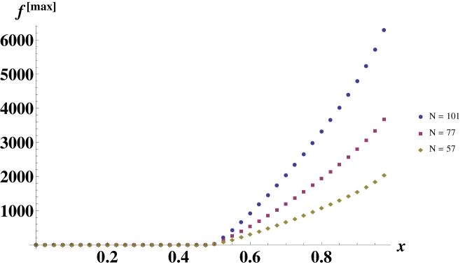
   Figure 3: Dependence of $f^{[\text{max}]}$ on temperature.

3. We used $f^{[\text{max}]}_{N,x}$ to extract the dependence of $\log(Z(N,x))$ to leading order in $N$. We did this by fitting this data set onto a model function:

   $$F(N,x)=c_{1}(x)N^{2}+c_{2}(x)N\log(N)+c_{3}(x)N+c_{4}(x)\log(N)+c_{5}(x)$$ (27)

   The form of $F(N,x)$ was decided by examining Eq. 16. The presence of the restricted double sum (Eq. 21) and the leading order behavior of $R_{N}$ imply a $N^{2}$ dependence of $F(N,x)$, the presence of $N!$ leads to the remaining $N$-dependent terms and the constant term is there to capture pure temperature dependence of $f^{[\text{max}]}_{N,x}$. We studied how these coefficients change with $x$ (or, temperature). FIG. 4 shows the temperature dependence of $c_{1}$.

   

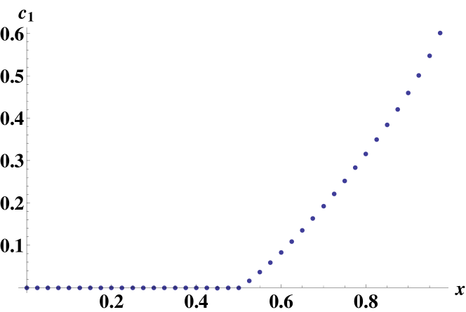
   Figure 4: The coefficient of $N^{2}$ in $\log{Z}$ switches on at $x=1/2$.

4. For each ($N,x$), we used $\{\psi_{k}\}_{N,x}$ to numerically approximate the density function of the global maxima, $\rho(\Psi)$ (Eq. 23). For $l\in\{1,\cdots,N-1\}$, we obtained

   $$\{\rho_{l}\}_{N,x}=\frac{1}{N-1}\frac{1}{\left\{\psi_{l+1}-\psi_{l}\right\}_{N,x}}$$ (28)

   where the $1/(N-1)$ is for normalization of the distribution.

Error estimates

$\widetilde{f}(N,x,\{\theta_{k}\})$ has multiple maxima of different orders in the search space $(-\pi,\pi)^{N-1}$. Locating a maximum isn’t as difficult as is ensuring that it is also a global maximum. We examined four different optimization methods and picked the best one for obtaining our final data set. A (nonlinear) least-squares fit of $F(N,x)$ was obtained to the data set. Of the $40$ fits, $38$ had an Adjusted $R^{2}$ value of $1$ while two of them had $0.98$ and $0.90$, respectively.

VI Results and Conclusions

In FIG. 3 we make an important observation: for $x<1/2$, $\log(Z)$ is independent of $N$ at leading order. The $N$-dependence sets in only for $x>1/2$. For $x>1/2$, the curves are concave upwards and diverge at $x=1$. Also, as $N$ gets larger, the curve gets steeper. At $N\rightarrow\infty$, the curve is infinitely steep at $x=1/2$, and we see the Hagedorn phenomenon.

The most important result of this paper is FIG. 4. This plot shows the dependence of the leading order coefficient in Eq. 27 on temperature. $c_{1}$ is negligible below $x=1/2$. In fact, all the coefficients of $N$-dependent terms; i.e. $c_{1},c_{2},c_{3}$ and $c_{4}$ are negligible below $x=1/2$. We can actually confirm that there is no $N^{2}$ term in the expansion of $\log(Z)$ Curtright et al. (2017). Above $x=1/2$, $c_{1}$ is positive and increases monotonically with $x$ (or, temperature). However, it doesn’t keep increasing indefinitely. From Eq. 22 we expect $\lim_{x\rightarrow 1}c_{1}=\log(2)\approx 0.69$. We confirmed this limiting behavior by conducting a subsequent search with a finer grid near $x=1$.

FIG. 4 clearly demarcates the two temperature regimes we proposed in the previous section. At lower temperatures $\log(Z)$ has no diverging terms in $N$. Hence, at $N\rightarrow\infty$, it has a limit point. Above $x=1/2$, the leading order terms diverge as $N\rightarrow\infty$. It is this difference in behavior that manifests as the Hagedorn phenomenon as $N\rightarrow\infty$. However, this difference is present only in the leading order in $N$. As, has been shown earlier, the finite $N$ partition function; taken in its entirety, is smooth over $x\in(0,1)$. There is no indication of any discontinuity or non-differentiability at $x=1/2$. Its only divergence is at infinite temperature.

The $N^{2}$ dependence of $\log{Z}$ is related to the underlying degrees of freedom in the superstring bit system. It signals the liberation of the superstring bits from their singlet, polymeric states. In other words, there is deconfinement in this model at $x=1/2$. The Hagedorn phenomenon thus has an interpretation as a phase transition between polymeric, color singlet states and monomeric, color adjoint states. And in this interpretation, $c_{1}(x)$ plays the role of the order parameter. In order to obtain the form of $c_{1}(x)$ analytically, it is necessary to find the density of the global maxima,$\{\psi_{k}\}_{N,x}$, for $x>1/2$.

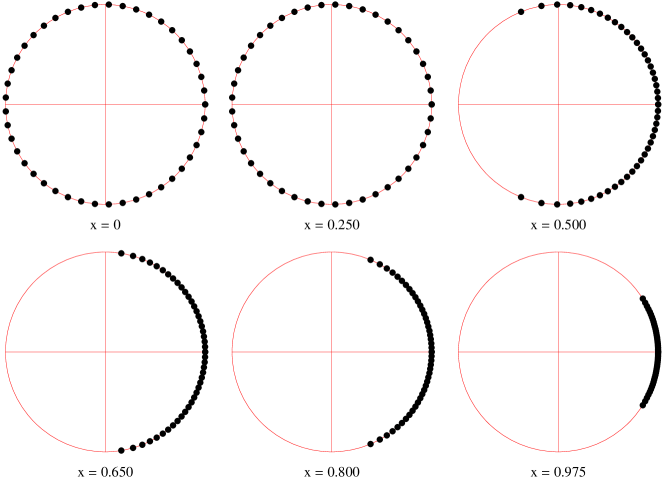
Figure 5: Distribution of the coordinates of the global maxima for $N=45$.

Speaking of $\{\psi_{k}\}_{N,x}$, this phase transition can also be detected by examining the distribution of the coordinates of the global maxima. In FIG. 5 we have plotted the temperature dependence of such distributions for $N=45$. These plots show a remarkable difference in the distribution of $\{\psi_{k}\}_{N,x}$ at different values of temperature. At low temperatures, the integrand is maximized by those regions in the domain where the $\{\psi_{k}\}_{N,x}$ are uniformly distributed in $(-\pi,\pi)$. It is as if the $\{\psi_{k}\}_{N,x}$, are repelling each other. This uniform distribution of of the coordinates is seen for all $x<1/2$. For $x\geqslant 1/2$, two things happen: the range of the distribution shrinks and the density peaks at its median. With increasing temperatures, the $\{\psi_{k}\}_{N,x}$ begin to attract each other, until at $x=1$, their distribution becomes a delta function. At infinite temperature, the integrand is maximized by those regions where the coordinates have the same value. This change in distribution of $\{\psi_{k}\}_{N,x}$ can be rationalized by noting that $\widehat{f}(0,\{\theta_{k}\})$ is a function of terms like $\sin^{2}\left(\frac{\theta_{i}-\theta_{j}}{2}\right)$ and $\widehat{f}(x\rightarrow 1,\{\theta_{k}\})$ contains terms like $\cos^{2}\left(\frac{\theta_{i}-\theta_{j}}{2}\right)$. However, it is interesting that this transition of the distribution doesn’t begin until $x=1/2$. One can construct the normalized density function from the $\{\psi_{k}\}_{N,x}$. FIG. 6 shows these density plots at different temperatures for $N=45$. Again, till $x=1/2$, the density function is a constant, with $\rho\approx 1/(2\pi)$. Above $x=1/2$, there exists a $\Psi_{[\text{max}]}<\pi$ such that $\rho\left(\pm\Psi_{[\text{max}]}\right)=0$ (Eq. 25). Such a cut-off for the density function has featured in previous studies of matrix models, e.g. the Hermitian matrix model Brézin et al. (1978).

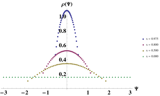
Figure 6: Normalized density function of the $\psi$s at different temperatures for $N=45$.

The change in the distribution of $\{\psi_{k}\}$ in our superstring bit model, bears a resemblance to the well-known phase transition in the unitary matrix model Gross and Witten (1980). While the latter has a coupling constant $g$, the parameter in our model is $x$, or the temperature. Still, there is a similarity in the transformation of the density functions: from low to high temperature in superstring bit model and from small to large coupling in the unitary matrix model. Recently, it was pointed out to us that Aharony et al obtained similar results for free $U(N)$ Yang-Mills theory with adjoint matter on $S^{3}\times\mathbb{R}$ Aharony et al. (2004). Both Sundborg Sundborg (2000) and Aharony et al. (2004) have obtained similar supersymmetric partition functions in the limit of large $N$. However, unlike in these models, an exact analytic expression of the high temperature density function still evades us.

Appendix A Gaussian approximation at infinite temperature

Let us Taylor-expand $\widehat{f}$ from Eq. 20 in {$\theta_{k}$}s about a global maximum at {$\psi_{k}$}:

$$\widehat{f}\left(x,\{\theta_{k}\}\right)=\widehat{f}\left(x,\{\psi_{k}\}\right)+\frac{1}{2}\sum_{r,s}(\theta_{r}-\psi_{r})\frac{d^{2}}{d\theta_{r}d\theta_{s}}\widehat{f}\left(x,\{\psi_{k}\}\right)(\theta_{s}-\psi_{s})+\cdots$$ (29)

$$\implies\int_{-\pi}^{\pi}\exp\widehat{f}\left(x,\{\theta_{k}\}\right)\prod_{1\leqslant l\leqslant N}d\theta_{l}\approx\mathcal{J}(N,x)\exp\left\{\widehat{f}\left(x,\{\psi_{k}\}\right)\right\}\int_{-\infty}^{\infty}\exp\left\{\frac{1}{2}\sum_{r,s}(\theta_{r}-\psi_{r})\frac{d^{2}\widehat{f}\left(x,\{\psi_{k}\}\right)}{d\theta_{r}d\theta_{s}}(\theta_{s}-\psi_{s})\right\}\prod_{1\leqslant l\leqslant N}d\theta_{l}=\mathcal{J}(N,x)\exp\left\{\widehat{f}\left(x,\{\psi_{k}\}\right)\right\}\sqrt{\frac{(2\pi)^{N}}{\text{det}(H)}}$$ (30)

where $\mathcal{J}(N,x)$ is the number of global maxima in $(-\pi,\pi)^{N}$ and

$$H_{rs}=-\frac{d^{2}}{d\theta_{r}d\theta_{s}}\widehat{f}\left(x,\{\psi_{k}\}\right)$$

As the integrand is translation invariant in the $\theta$s, $\mathcal{J}(N,x)$ is $\infty$. As we shall see later, the correct approximation involves applying steepest descent after removing the zero mode integral. Once the zero mode is removed, $\mathcal{J}(N,x)$ is the number of global maxima in $(-\pi,\pi)^{N-1}$. $\mathcal{J}(N,x)$ in general has a factor of $(N-1)!$ coming from the symmetry of the integrand in the $\theta$s.

At infinite temperature ($x=1$) there is only one global maximum: $\psi_{1}=\psi_{2}=\cdots=\psi_{N}$. Hence, $\mathcal{J}(N,1)=1$ and from Eq. 18

$$Z(N,1)\approx\left(\frac{2}{1-x}\right)^{N-1}\frac{2^{N(N-1)}}{N!(2\pi)^{N}}\int^{\infty}_{-\infty}\exp\left\{-\frac{1}{2}\sum_{r,s}\underbrace{\frac{N\delta_{rs}-1}{2}}_{=H_{rs}}\theta_{r}\theta_{s}\right\}\prod^{N}_{k=1}d\theta_{k}$$ (31)

Here we can see that the formula for the Gaussian integral yields $\infty$. This is because we blindly replaced every one dimensional integration $\int_{-\pi}^{\pi}{d\theta_{i}\ \cdots}$ with $\int_{-\infty}^{\infty}{d\theta_{i}\ \cdots}$ when we took the Gaussian approximation. Hence, instead of obtaining a factor of $2\pi$ from the zero mode, we get $\infty$. The correct formula is

$$2\pi\sqrt{\frac{(2\pi)^{N-1}}{\text{det}(H^{\prime})}}$$

where $H^{\prime}_{rs}=H_{rs}\ \forall\{r,s\}\ \in\{1,2,\cdots,N-1\}$. $H^{\prime}$ is the $(N-1)\times(N-1)$ matrix one gets after truncating the $N^{\text{th}}$ row and $N^{\text{th}}$ column of $H$. Evaluating $\text{det}(H^{\prime})$ we get $\frac{N^{N-2}}{2^{N-1}}$. Putting everything back into the earlier equation we get

$$Z\approx\left(\frac{2}{1-x}\right)^{N-1}\frac{2^{N(N-1)}}{N!(2\pi)^{N}}2\pi\sqrt{\frac{2^{N-1}(2\pi)^{N-1}}{N^{N-2}}}=\left(\frac{2}{1-x}\right)^{N-1}\frac{1}{N!}\frac{2^{N(N-1)}}{\pi^{(N-1)/2}N^{N/2-1}}$$ (32)

We can compare this to Eq. 18 to infer:

$$R_{N}=\sum_{\Gamma}{\text{Res}\left(\frac{\prod_{1\leqslant i<j\leqslant N}(z_{i}+z_{j})^{2}}{\prod_{1\leqslant k\leqslant N}(z_{k})^{N}}\right)}\approx\frac{2^{N(N-1)}}{\pi^{(N-1)/2}N^{N/2-1}}$$ (33)

While searching through mathematics literature, we came to know that $R_{N}$ as defined above, also counts the number of Eulerian digraphs with $N$ nodes McKay (1983). Also, the author lists exact values of $R_{N}$ till $N=16$, some of which we have used in FIG. 2. A follow up on our search revealed that the asymptotic expression in Eq. 33 has already been computed in McKay (1990). It turns out that multiplying our Gaussian result with an extra factor of $e^{-1/4}$ is a more accurate approximation in leading order.

References

- Giles and Thorn (1977) Roscoe Giles and Charles B. Thorn, “Lattice approach to string theory,” Physical Review D 16, 366–386 (1977).
- Hooft (1974) G. ’t Hooft, “A planar diagram theory for strong interactions,” Nuclear Physics B 72, 461–473 (1974).
- Thorn (1994) Charles B. Thorn, “Reformulating String Theory with the $1/N$ Expansion,” arXiv:hep-th/9405069 (1994), arXiv: hep-th/9405069.
- Bergman and Thorn (1995) Oren Bergman and Charles B. Thorn, “String bit models for superstring,” Physical Review D 52, 5980–5996 (1995).
- Thorn (2014) Charles B. Thorn, “Space from string bits,” Journal of High Energy Physics 2014, 1–24 (2014).
- Hagedorn (1965) R. Hagedorn, “Statistical thermodynamics of strong interactions at high-energies,” Nuovo Cim.Suppl. 3, 147–186 (1965).
- Fubini and Veneziano (1969) S. Fubini and G. Veneziano, “Level structure of dual-resonance models,” Il Nuovo Cimento A (1971-1996) 64, 811–840 (1969).
- Atick and Witten (1988) Joseph J. Atick and Edward Witten, “The Hagedorn transition and the number of degrees of freedom of string theory,” Nuclear Physics B 310, 291–334 (1988).
- Thorn (2015) Charles B. Thorn, “String bits at finite temperature and the Hagedorn phase,” Physical Review D 92 (2015), 10.1103/PhysRevD.92.066007.
- Sun and Thorn (2014) Songge Sun and Charles B. Thorn, “Stable string bit models,” Physical Review D 89, 105002 (2014).
- Chen and Sun (2016) Gaoli Chen and Songge Sun, “Numerical study of the simplest string bit model,” Physical Review D 93, 106004 (2016).
- Aharony et al. (2004) Ofer Aharony, Joseph Marsano, Shiraz Minwalla, Kyriakos Papadodimas, and Mark Van Raamsdonk, “The Hagedorn/Deconfinement Phase Transition in Weakly Coupled Large N Gauge Theories,” Advances in Theoretical and Mathematical Physics 8, 603–696 (2004).
- Sundborg (2000) Bo Sundborg, “The Hagedorn transition, deconfinement and N=4 SYM theory,” Nuclear Physics B 573, 349–363 (2000).
- Curtright et al. (2017) Thomas L. Curtright, Sourav Raha, and Charles B. Thorn, “Color Characters for White Hot String Bits,” arXiv:1708.03342 [hep-th] (2017), arXiv: 1708.03342.
- Weyl (1946) Hermann Weyl, The Classical Groups, Their Invariants and Representations (Princeton University Press, Princeton, N.J., 1946).
- Curtright and Thorn (1986) Thomas L. Curtright and Charles B. Thorn, “Symmetry patterns in the mass spectra of dual string models,” Nuclear Physics B 274, 520–558 (1986).
- McKay (1983) Brendan D. McKay, “Applications of a technique for labelled enumeration,” Congressus Numerantium 40, 207–221 (1983).
- Brézin et al. (1978) E. Brézin, C. Itzykson, G. Parisi, and J. B. Zuber, “Planar diagrams,” Communications in Mathematical Physics 59, 35–51 (1978).
- Gross and Witten (1980) David J. Gross and Edward Witten, “Possible third-order phase transition in the large-$N$ lattice gauge theory,” Physical Review D 21, 446–453 (1980).
- McKay (1990) Brendan D. McKay, “The asymptotic numbers of regular tournaments, Eulerian digraphs and Eulerian oriented graphs,” Combinatorica 10, 367–377 (1990).