Efficient, High-Quality Stack Rearrangement

Abstract

This work studies rearrangement problems involving the sorting of robots or objects in stack-like containers, which can be accessed only from one side. Two scenarios are considered: one where every robot or object needs to reach a particular stack, and a setting in which each robot has a distinct position within a stack. In both cases, the goal is to minimize the number of stack removals that need to be performed. Stack rearrangement is shown to be intimately connected to pebble motion problems, a useful abstraction in multi-robot path planning. Through this connection, feasibility of stack rearrangement can be readily addressed. The paper continues to establish lower and upper bounds on optimality, which differ only by a logarithmic factor, in terms of stack removals. An algorithmic solution is then developed that produces suboptimal paths much quicker than a pebble motion solver. Furthermore, informed search-based methods are proposed for finding high-quality solutions. The efficiency and desirable scalability of the methods is demonstrated in simulation.

I Introduction

Many robotic applications involve the handling of multiple stacks. For instance, spatial restrictions faced by growing urban areas already motivate stackable parking lots for vehicles, as in Fig. 1(a). With the advent of autonomous vehicles, such solutions will become increasingly popular and will require automation. Similarly, products in convenience stores are frequently arranged in “gravity flow” shelving units depending on their type, as in Fig. 1(b). Such stacks of products and materials arise in the industry where a robot is able to interact with the foremost object and perform operations similar to a “push” or a “pop” of a stack data structure.

In the above stack rearrangement setups, the objective may be to remove a specific object from the stack (e.g., a specific car from the stackable parking) or to rearrange the objects into a specific arrangement, which specifies the location of each object within a stack (e.g., a Hanoi tower-like setting). High quality solutions are highly desirable for the applications, especially with regards to the number of stack removals. Otherwise, an exorbitant amount of time is spent performing redundant actions, which reduces efficiency or appears unnatural to people.

Through a reduction to the pebble motions problem, which is well-studied in the multi-robot literature, the feasibility of stack rearrangement can be readily decided. A naive feasible solution, however, can be far from optimal in minimizing stack removals. Adapting a divide-and-conquer technique, this paper establishes lower and upper bounds on this number that differ by a mere logarithmic factor. Results are provided both for objects that need to be placed in the right stack as well as the more general case where objects need to acquire a specific position in the stack. Finally, the paper considers both optimal and sub-optimal informed search methods and proposes effective heuristics for stack rearrangement. This leads to an experimental evaluation of the different algorithms and heuristics, which suggests a combination that scales nicely with the number of stackable objects.

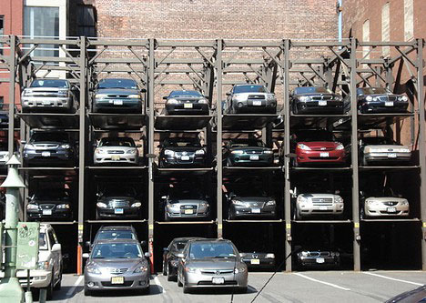
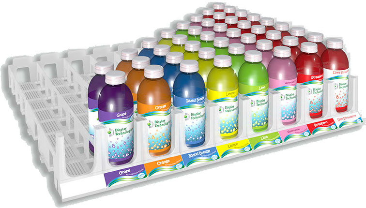
Figure 1: (a) Stackable parking lots are expected to become even more popular in urban environments with the advent of autonomous vehicles. (b) Rearranging stacks of objects is a task frequently encountered in convenience and grocery stores.

Related Work: Multi-body planning is itself hard. In the continuous case, complete approaches do not scale even though methods try to decrease the effective DOFs [1]. For specific geometries, e.g., unlabeled unit-discs among polygons, optimality is possible [29], even though the unlabeled case is still hard [28]. Given the problem’s hardness, decoupled methods, such as priority-based schemes [33] or velocity tuning [19], trade completeness for efficiency.

Recent progress has been achieved for the discrete problem variant, where robots occupy vertices and move along edges of a graph. For this “pebble motion on a graph” problem [14, 4, 2, 10], feasibility can be answered in linear time and paths can be acquired in polynomial time [17, 20, 35, 37]. The optimal variation is still hard but recent optimal solvers with good practical efficiency have been developed [35, 37, 26, 38]. The current work is motivated by this progress and aims to show that for stack rearrangement it is possible to come up with practically efficient algorithms.

General rearrangement planning [3, 22] is also hard, similar to the related “navigation among movable obstacles” (NAMO) [36, 5, 6, 21, 34], which can be extended to manipulation among movable obstacles (MAMO) and related challenges [32, 13, 30, 7, 18, 15, 16]. These efforts focus on feasibility and no solution quality arguments have been provided. A recent work has focused, similar to the current paper, on high-quality rearrangement solutions but in the context of manipulation challenges in tabletop environments [11].

II Problem Formulation

Assume $n$ objects ${\mathcal{O}}=\{o_{1},\ldots,o_{n}\}$ that occupy $w+1$ last-in-first-out (LIFO) queues, i.e., stacks, where $w\geq 2$, since 2-stack rearrangement is impossible. Elements can only be added or removed from one end of the data structure, often referred to as the “top”. Furthermore, each stack has an integer depth of $d\geq 1$, corresponding to the maximum stack capacity. An object at the top of a stack has a depth of $1$. The assumption is that $n\leq wd$, unless specified otherwise.

Modeling many real world problems, the assumption is that objects in a stack always occupy contiguous positions, e.g., if the top object is removed from a stack in Fig. 1(b), the remaining objects in the stack will “slide” to the front. Similarly, as an object is pushed onto a stack, the existing objects will shift backwards by one position. It is straightforward to see that the two versions of the problem, i.e., a top-down or a bottom-up stack, as shown in Fig. 2, induce the same problem. For consistency, the bottom-up setting is used for the remainder of the paper.

(a) Top-down		(b) Bottom-up

Figure 2: Visualization of the abstract problem where objects (a) slide to the front of the stacks, (b) are pulled to the bottom of the stack.

Using this setup, an object that currently resides at the top of stack $i$ can be transferred to an arbitrary stack $j$ via a pop-and-push action, denoted as $a_{ij}$. A permissible pop-and-push action constrains the above definition by requiring that $i$ be non-empty, and that $j$ not currently be at capacity.

An arrangement is an injective mapping $\pi:\mathcal{O}\to\mathbb{N}^{2}$, $o_{i}\mapsto\pi(o_{i})$. Here, $\pi(o_{i})$ is a 2-tuple $(\pi^{1}(o_{i}),\pi^{2}(o_{i}))$ in which $1\leq\pi^{1}(o_{i})\leq w$ and $1\leq\pi^{2}(o_{i})\leq d$ are the stack and depth locations of $o_{i}$, respectively. The paper primarily focuses on two main problems, defined as follows.

Problem 1.

Labeled Stack Rearrangement (LSR). Given $\langle{\mathcal{O}},w,d,\pi_{I},\pi_{G}\rangle$, compute a sequence of pop-and-push actions $A=(a_{i_{1}j_{1}},a_{i_{2}j_{2}},\dots)$ that move the objects one at a time from an initial $\pi_{I}$ to a goal arrangement $\pi_{G}$.

Problem 2.

Column-Labeled Stack Rearrangement (C-LSR). Similar to LSR, but the objects are only required to be moved to their goal stacks without a specific depth. That is, $\pi_{G}^{2}$ is left unspecified for all objects.

Whereas C-LSR can be viewed as a sub-problem in approaching LSR, it has practical incarnations - perhaps even more so than LSR. For example, in retail, it is almost always the case that a shelf slot holds the same type of product (e.g., Fig. 1(b)). Solving C-LSR then corresponds to rearranging an out of order shelf so that each stack holds only a single type of product.

In this paper, the optimization objective is to minimize the number of actions taken, i.e. $|A|$. For robotic manipulation, the objective models the required number of grasps by the robotic manipulator, which is frequently the limiting factor.

III Structural Analysis

A closely related problem is Pebble Motion on Graphs (PMG) [14]: suppose an undirected graph $G=(V,E)$ has $p<|V|$ pebbles placed on distinct vertices and which can move sequentially to adjacent empty vertices. Given a PMG instance $\langle G,x_{I},x_{G}\rangle$, the goal of PMG is to decide if the configuration $x_{G}$ is reachable from $x_{I}$, and to subsequently find a sequence of moves to do so when possible. When $G$ is a tree, this problem is referred to as Pebble Motion on Trees (PMT). The considered versions of LSR (and C-LSR) are PMT problems.

(a) An LSR instance		(b) A PMT instance

Figure 3: From LSR to PMT

Proposition III.1.

An LSR instance is always reducible to a PMT instance. In particular, a solution to the reduced PMT instance is also a solution to the initial LSR instance.

Proof.

Given an LSR instance $\langle{\mathcal{O}},w,d,\pi_{I},\pi_{G}\rangle$, as shown in Fig. 3, the tree graph $T=(V,E)$ in the PMT instance is obtained by first viewing each stack as a path of length $d$, and then joining the top vertices of these stacks with a root vertex, which builds the connection between them. This yields $|V|=((w+1)d)+1$ vertices. It is clear that object arrangements $\pi_{I}$ and $\pi_{G}$ directly map to configurations $x_{I}$ and $x_{G}$ of a PMT instance. Note that a pop-and-push action in the LSR solution is equivalent to moving one pebble from a path on $T$ to another path through the root vertex. Similarly, given a solution to the PMT instance, a solution to the LSR instance can be constructed by treating a pebble passing through the root as a pop-and-push action. ∎

Given the relationship between PMT and LSR, and that finding optimal solutions (i.e., a shortest solution sequence) for PMG and many of its variants is NP-hard [9, 25], there is evidence to believe that optimally solving LSR (i.e., minimizing the number of actions) is also NP-hard.

In terms of feasibility, the LSR problem is always feasible as defined. This is due to the assumption that $n\leq wd$ while the total number of slots in the stacks are $(w+1)d$. This allows to always clear one stack of depth $d$ and then the elements in the remaining stacks can be arranged with the aid of the empty one. Consider, however, a more general version, called GLSR, that allows for $n$ to exceed $wd$. So there may be fewer than $d$ buffers available to rearrange objects.

Note that Proposition III.1 still holds for GLSR. The mapping from GLSR to PMT immediately leads to algorithmic solutions for GLSR (and therefore, LSR). By Proposition III.1, a GLSR instance is feasible if and only if the corresponding PMT instance is so. The feasibility test of PMT can be performed in linear time [2], so the same is true for GLSR as the reduction can be performed also in linear time.

For a feasible GLSR, solving the corresponding PMT can be performed in $O(|V|^{3})$ running time (and pebble moves) [14]. This translates to a solution for GLSR that runs in $O(w^{3}d^{3})$ time using up to $O(w^{3}d^{3})$ actions. This result, however, does not extend to LSR (i.e., when $n\leq wd$) as an LSR instance is in fact always feasible. It turns out that LSR can be solved in less computation time and a reduced number of actions than using a PMT solver. This contribution is established in the following proposition.

Proposition III.2.

An arbitrary LSR can be solved using $O(wd^{2})$ pop-and-push actions.

Proof.

Consider an LSR with $n=wd$. Without loss of generality, assume that: $\forall\ o\in\mathcal{O}:\pi_{I}^{1}(o)\leq w,\pi_{G}^{1}(o)\leq w,$ i.e., stack $w+1$ is empty at the start and goal state. It suffices to show that one stack (e.g., the first) can be arranged in $O(d^{2})$ actions and this can be repeated $w$ times. The $O(d^{2})$ cost for a stack is because each object can be moved to its destination in $O(d)$ moves and this can be repeated for $d$ times. Consider the object $o$ to be moved at the bottom of the first stack, i.e., $\pi_{G}(o)=(1,d)$. Without loss of generality, assume that $\pi_{I}(o)=(x,y)$ with $x\neq 1$. Initially, $o$ will be moved to the top of stack $x$. If $y=1$, no action is needed. Otherwise, perform the following moves per Fig. 4: (i) move the object at $(1,1)$ to the buffer stack $(w+1)$, (ii) move objects from $(x,1)$ to $(x,y-1)$ to the buffer, (iii) move $o$ to $(1,1)$, (iv) move all objects in the buffer except the last to stack $x$, (v) move $o$ to the top of stack $x$, and (vi) move the last object in the buffer to stack $1$.

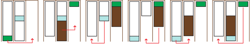
Figure 4: The cyan object moves to the top of its stack $x$ with $O(d)$ actions.

Using the same $O(d)$ procedure, the object $o^{\prime}$ at $(1,d)$ can be moved to $(1,1)$. Using the buffer stack $(w+1)$, $o$ and $o^{\prime}$ can be swapped in three actions. Then, reverting the sequences, $o$ can be moved to $(1,d)$ for an $O(d)$ total number of actions . So, arranging a single stack needs $O(d^{2})$ actions and the entire problem takes $O(wd^{2})$ actions. ∎

The running time is also bounded by $O(wd^{2})$ since the only computation cost is to go through $\pi_{I}$ and $\pi_{G}$ and recover the solution sequence. For GLSR, which allows $n>wd$, an arbitrary instance may not be feasible. This paper focuses on the optimal number of actions for rearrangement problems, so GLSR is not considered further.

IV Fundamental Bounds on Optimality

This section provides an analysis on the structure properties of LSR, focusing on the fundamental optimality bounds and polynomial time algorithms for computing them. The analysis assumes the hardest case of LSR where $n$ equals $wd$. Without loss of generality, it is assumed that stack $(w+1)$ is empty at the initial and goal state, serving as a buffer. First, consider the lower bound on the number of required actions.

Proposition IV.1.

In the average case, $\Omega(wd)$ actions are required for solving LSR.

Proof.

First consider a worst case scenario, i.e., that the deepest objects $o_{i}\in\mathcal{O}$ in each stack $k$, i.e., $\pi_{I}(o_{i})=(k,d)$, must be moved to the next stack $k+1$ modulo $w$, i.e., $\pi_{G}(o_{i})=((k+1)\mod\ w,d)$. To move each of these objects, at least $d$ actions are needed because $d-1$ objects are blocking the way to them. Therefore, the total number of required actions is $\Omega(wd)$.

In the average case (assuming $\pi_{I}$ and $\pi_{G}$ are both uniformly randomly generated), for each stack $k$, $1\leq k\leq w$, look at an object along the stack. Each object $o$ has probability $(w-1)/w$ to have $\pi_{I}^{1}(o)\neq\pi_{G}^{1}(o)$. That is, with probability $1/w$, $o$ will stay in stack $k$ and with probability $(w-1)/w$ it must be moved to a different stack. Because moving $o$ will require on average $d/2$ actions, the expected cost of moving it is then $(w-1)d/(2w)$. For all $w$ stacks, this is then $\Omega((w-1)wd/(2w))=\Omega(wd)$. ∎

For the case of $w\ll d$, better average case lower bounds can be found per the following lemma.

Lemma IV.1.

The number of moves for solving LSR is $\Omega(wd\log d/\log w)$.

Proof.

The bound is established by counting the possible LSR problems for fixed $w$ and $d$, i.e., for the case $n=wd$. Given a fixed $\pi_{I}$, there are $n!$ possible $\pi_{G}$, so there are at least $n!=(wd)!$ different LSR instances. With each action, one object at the top of a stack ($w+1$ of these) can be moved to any other stack ($w$ of these). Therefore, each action can create at most $w(w+1)<(w+1)^{2}$ new configurations. In order to solve all possible LSR instances, it must then be the case that the required number of moves, defined as $\min\{|A|\}$, must satisfy $[(w+1)^{2}]^{\min\{|A|\}}\geq(wd)!$. Then, by Sterling’s approximation, $\min\{|A|\}=\Omega(wd\frac{\log d}{\log w})$. ∎

Lemma IV.1 implies Proposition IV.1 as well but does so in a less direct way. Interestingly, Lemma IV.1 immediately implies the following better lower bounds.

Corollary IV.1.

For an LSR with $w=e^{\sqrt{\log d}}$, on average it requires $\Omega(wd\sqrt{\log d})$ actions to solve.

Corollary IV.2.

For an LSR with $w$ being a constant, on average it requires $\Omega(d\log d)$ actions to solve.

The focus now shifts towards upper bounds on optimality where polynomial time algorithms are presented for computing them. Recall that a trivial upper bound of $O(wd^{2})$ is given by Proposition III.2. Comparing the $O(wd^{2})$ upper bound with the lower bound, which ranges between $\Omega(wd)$ and $\Omega(d\log d)$ (for constant $w$), there remains a sizable gap. Forthcoming algorithms illustrate how to significantly reduce, and in certain cases eliminate this gap.

Lemma IV.2.

An arbitrary instance of C-LSR can be solved using $O(wd\log w)$ actions.

Proof.

The $\log w$ factor in $O(wd\log w)$ comes from a divide-and-conquer approach. As such, a recursive algorithm is outlined for solving C-LSR. In the first iteration, partition all $wd$ objects into two sets based on $\pi_{G}^{1}$. For an object $o\in\mathcal{O}$, if $\pi_{G}^{1}(o)\leq\lceil w/2\rceil$, then it is assigned to the left set. Otherwise it is assigned to right set. The goal of the first iteration is to sort objects so that the left set resides in stacks $1$ to $\lceil w/2\rceil$, as illustrated in Fig. 5.

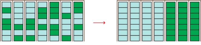
Figure 5: The goal of the first iteration in solving an C-LSR instance with $w=7$ and $d=7$. The empty stack is not drawn.

In the first iteration, begin with the first stack and sort it into two contiguous sections belonging to the left set and the right set. The process involves using another occupied stack and the buffer stack (using $O(d)$ moves). Note that the content of the other occupied stack is irrelevant. These three stacks are illustrated in the first figure in Fig. 6. Assume that $\ell$ objects of stack $1$ belong to the left set (in the example, $\ell=4$). To begin, the top $\ell$ objects of the last stack is moved to the buffer. This allows the sorting of the first stack into two contiguous blocks of left only and right only objects, which can then be returned to the first stack. Note that the order of the two blocks can be reversed using the same procedure; this will be used shortly. The procedure is then applied to all stacks. The procedure and the end result are illustrated in Fig. 6. It is clear that the total actions required is $O(wd)$.

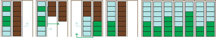
Figure 6: The left four figures illustrate the process of sorting a single stack into two contiguous blocks. The last figure is the end result of applying the procedure to all stacks.

The next step involves the first two stacks and attempts to consolidate the sets. If any stack is already fully occupied by either the left or the right set, then that stack can be skipped; suppose not. Let these two stacks be $i$-th and $j$-th stacks and let $\ell_{i}$ and $\ell_{j}$ be the number of objects belonging to the left set in the $i$-th and $j$-th stacks, respectively. If $\ell_{i}+\ell_{j}\geq d$, then using the buffer stack, stack $i$ can be forced to contain only objects belonging to the left set. Fig. 7 illustrates applying the procedure to the left most two stacks to the running example and the result.

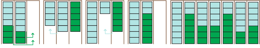
Figure 7: Consolidating the first two stacks.

If $\ell_{i}+\ell_{j}<d$, then stack $i$ is processed so that the $\ell_{i}$ objects belonging to the left set are on the top (using the block reverse procedure mentioned earlier in this proof). Then, a similar consolidation routine can be applied. Fig. 8 illustrates the application of the procedure to stacks $2$ and $3$ of the right most figure of Fig. 7. With these two variations, all stacks can be sorted so that each stack contains only objects from either the left set or the right set.

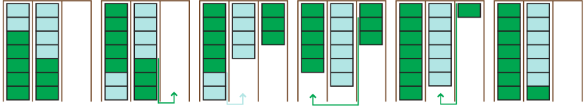
Figure 8: Consolidating the first two stacks that requires reversing the two contiguous blocks one of the two stacks.

At this point, using the buffer stack, entire stacks can be readily swapped to complete the first iteration. The total number of actions used is $O(wd)$ per iteration. Applying the same iterative procedure to the left and the right sets of objects, the full C-LSR problem can then be solved with $O(wd\log w)$ actions. ∎

After solving C-LSR, each stack needs to be resorted to fully solve the original LSR problem, which can be performed using $O(d\log d)$ actions.

Lemma IV.3.

After solving the C-LSR portion of an LSR instance, a stack can be fully sorted using another stack and the buffer stack with $O(d\log d)$ actions.

Proof.

The sorting is done recursively. Suppose stack $i$ is to be sorted using stack $j$ and the buffer stack. Assume without loss of generality that $d=2^{k}$ for some $k$. To start, move half of the objects in stack $j$ to the buffer stack. This creates two buffers of size $2^{k-1}$. Using these two buffers, stack $i$ can be sorted into a top half and a bottom half. As these two halves are restored to stack $i$, the top and bottom halves are separated. Iteratively applying the same procedure can then sort stack $i$ fully in $\log d$ iterations. The total number of required actions is then $O(d\log d)$. Fig. 9 provides an illustrative example sorting sequence for $k=3$. ∎

\begin{overpic}[width=433.62pt]{sor} \put(7.5,24.75){\footnotesize(a)} \put(27.75,24.75){\footnotesize(b)} \put(48.25,24.75){\footnotesize(c)} \put(68.25,24.75){\footnotesize(d)} \put(88.75,24.75){\footnotesize(e)} \put(7.5,-1.0){\footnotesize(f)} \put(27.75,-1.0){\footnotesize(g)} \put(48.0,-1.0){\footnotesize(h)} \put(68.5,-1.0){\footnotesize(i)} \end{overpic}

Figure 9: An example of sorting a stack with $d=2^{3}$.

Lemma IV.2 and Lemma IV.3 suggest that the gap between the lower and upper bounds for LSR can be completely eliminated for constant $w$.

Theorem IV.1.

For constant $w$, LSR can be solved using $O(d\log d)$ actions, agreeing with the $\Omega(d\log d)$ lower bound.

Proof.

By Lemma IV.2, when $w$ is a constant, a corresponding C-LSR problem can be solved using $O(wd\log w)=O(d)$ actions. Lemma IV.3 then applies to do the final sorting in $O(wd\log d)=O(d\log d)$ actions. The total number of required actions is then $O(d\log d)$. The lower bound is given by Corollary IV.2. ∎

The following provides a tighter upper bound for non-constant $w$.

Theorem IV.2.

An arbitrary LSR instance can be solved using $O(wd\max\{\log d,\log w\})$ actions.

Proof.

Applying Lemma IV.2 to the LSR problem yields a stack sorted instance of LSR using $O(wd\log w)$ actions. Since sorting each of the stacks afterward takes $O(d\log d)$ time, the full LSR problem can be solved using $O(wd\max\{\log d,\log w\})$ actions. ∎

The greatly improved and general upper bound is now fairly close to the general lower bound $\Omega(wd)$ within only a logarithmic factor.

1 Poly-C-LSR$(1,w)$

2 for $c_{i}\in[1,w]$ do Sort stack $c_{i}$

3 return

4

5 Function  Poly-C-LSR$(l,r)$

6       if  $l=r$ then return

7       $i\leftarrow l,j\leftarrow r,m\leftarrow\lfloor(l+r)/2\rfloor$

8       for $o_{i}\in O$ do

9             if $l\leq\pi^{1}_{G}(o_{i})\leq m$ then label $o_{i}$: left

10             else if $m+1\leq\pi^{1}_{G}(o_{i})\leq r$ then label $o_{i}$: right

11            

12      for $c_{i}\in[l,r]$ do Reorder stack $c_{i}$

13       for $c_{i}\in[l,r]$ do Consolidate stack $c_{i}$

14       Poly-C-LSR$(l,m)$

15       Poly-C-LSR$(m+1,r)$

16       return

17      

Algorithm 1 Poly-LSR$(\pi_{I},\pi_{G})$

The algorithmic process (Poly-LSR) for the method introduced above is shown in Alg. 1. It contains the subroutine for solving C-LSR  (Poly-C-LSR, in line 1-1), which iteratively separates the left and right objects in each stack (line 1), and consolidate the stacks (line 1). Details are already mentioned in Lemma IV.2. LSR is solved by first calling Poly-C-LSR and then sorting all the stacks using the routine in Lemma IV.3 (line 1). The overall time complexity is $O(wd~{}\max\{\log~{}d,\log~{}w\})$, which is equivalent to the number of steps in the generated solution.

V Optimal and Sub-optimal LSR Solvers

LSR can be reduced to a Shortest Path Problem, which searches for a minimum weight path between two nodes in an undirected graph. Here a node simply denotes an arrangement $\pi$. The neighbors of this node are all the arrangements reachable from $\pi$ via a single pop-and-push action. The edge weights between connected nodes are uniform.

The A* search algorithm[12] is a common tool for solving such a problem optimally. The branching factor is $(w+1)w$ since a pop-and-push action picks an object from one of $(w+1)$ stacks, and places it in one of the other $w$ stacks. Several heuristic functions are designed to guide the search:

Depth Based Heuristic (DBH). This heuristic returns an admissible number of pop-and-push actions needed to move $o_{i}\in{\mathcal{O}}$ to its goal. The detailed process appears in Alg. 2. It initially checks if $o_{i}$ is at its goal location (line 2), and simply returns $0$ if this statement is true. Lines 2 and 2 calculate the number of objects in front of $o_{i}$ in $\pi_{C}$ (resp. $\pi_{G}$), and denote it as $n_{c}$ (resp. $n_{g}$). At this point (line 2), if the object is currently in its goal stack, DBH computes the estimated number of moves via the following process: (1) take $o_{i}$ out of $\pi_{G}(o_{i})$, (2) make the goal pose reachable by inserting/removing intermediary objects from $\pi_{G}(o_{i})$, and (3) place $o_{i}$ back into $\pi_{G}(o_{i})$. If the object is not in its goal stack, then one of the following apply: If $\pi_{G}(o_{i})$ is reachable from $\pi_{C}(o_{i})$ solely by removing intermediary objects in front of both locations, then the object can be moved in $n_{c}+n_{g}+1$ steps; Otherwise, $o_{i}$ needs to be moved to an intermediate stack and this induces an extra move.

1 if $\pi_{C}(o_{i})=\pi_{G}(o_{i})$ then return 0

2 $n_{c}\leftarrow|\{o_{j}|o_{j}\in{\mathcal{O}},\pi_{C}^{1}(o_{j})=\pi_{C}^{1}(o_{i}),\pi_{C}^{2}(o_{j})<\pi_{C}^{2}(o_{i})\}|$

3 $n_{g}\leftarrow|\{o_{j}|o_{j}\in{\mathcal{O}},\pi_{G}^{1}(o_{j})=\pi_{G}^{1}(o_{i}),\pi_{G}^{2}(o_{j})<\pi_{G}^{2}(o_{i})\}|$

4 if $\pi_{C}^{1}(o_{i})=\pi_{G}^{1}(o_{i})$ then

5       if $n_{c}>n_{g}$ then return $2n_{c}-n_{g}+2$

6       else return $n_{g}+2$

7      

8else

9       if $\pi_{C}^{2}(o_{i})+\pi_{G}^{2}(o_{i})-1\leq(w+1)d-n$ then

10            return $n_{c}+n_{g}+1$

11      else return $n_{c}+n_{g}+2$

12      

Algorithm 2 DBH($o_{i},\pi_{C},\pi_{G}$)

The following variants of DBH deal with multiple objects:

1. DBH1: admissible, takes the maximum DBH value over all objects: $h_{\text{DBH1}}=\max\nolimits_{o\in{\mathcal{O}}}\text{DBH}(o,\pi_{C},\pi_{G})$.

2. DBHn: inadmissible, takes the summation of DBH values: $h_{\text{DBHn}}=\sum\nolimits_{o\in{\mathcal{O}}}\text{DBH}(o,\pi_{C},\pi_{G})$.

Column Based Heuristic (CBH). Described in Alg. 3, CBH counts the summation of the minimum number of actions necessary to move each object to its goal stack. As opposed to DBH which seeks a tight estimate for a single object, CBH considers all objects.

The detailed process is as follows. For every object $o_{i}\in{\mathcal{O}}$, CBH first determines whether $\pi_{C}^{1}(o_{i})=\pi_{G}^{1}(o_{i})$ (line 3). If $\pi_{C}^{1}(o_{i})=\pi_{G}^{1}(o_{i})$, the heuristic value $h$ remains unchanged if the objects behind $o_{i}$ are all at their goals. Otherwise, there exists either an object currently deeper than $o_{i}$ that needs to be evacuated, or an object in another stack that needs to be inserted to $\pi^{1}_{G}(o_{i})$ at a depth deeper than $\pi^{2}_{G}(o_{i})$. Thus $o_{i}$ must be taken out of its goal stack. This requires two additional actions (line 3).

If $\pi_{C}^{1}(o_{i})\neq\pi_{G}^{1}(o_{i})$, it takes at least 1 action for $o_{i}$ to be moved to $\pi^{1}_{G}(o_{i})$ (line 3). However if the empty locations in the stacks other than $\pi^{1}_{C}(o_{i})$ and $\pi^{1}_{G}(o_{i})$ cannot contain all the objects in front of $\pi_{C}(o_{i})$ and $\pi_{G}(o_{i})$, $o_{i}$ must be moved to an intermediate stack. This requires $2$ actions (line 3).

1 $h\leftarrow 0$

2 for  $o_{i}\in{\mathcal{O}}$ do

3       if $\pi^{1}_{C}(o_{i})$ = $\pi^{1}_{G}(o_{i})$  then

4             if $\exists o_{j}\in{\mathcal{O}},\pi^{1}_{C}(o_{j})=\pi^{1}_{C}(o_{i}),\pi^{2}_{C}(o_{j})>\pi^{2}_{C}(o_{i}),\pi_{C}(o_{j})\neq\pi_{G}(o_{j})$ then $h\leftarrow h+2$

5            

6      else

7             if $(w+1)d-n<\pi^{2}_{C}(o_{i})+\pi^{2}_{G}(o_{i})-1$ then $h\leftarrow h+2$

8             else $h\leftarrow h+1$

9            

10      

11return h

Algorithm 3 CBH($\pi_{C},\pi_{G}$)

An example of DBH and CBH calculation is shown in Fig. 10. The running time for DBH is $O(d)$, so totally $O(nd)$ for both DBH1 and DBHn. CBH runs in $O(n)$ time when dealing the objects in each stack in a bottom-up manner.

Figure 10: An example for heuristic calculation. The left figure denotes $\pi_{C}$, while the right one denotes $\pi_{G}$. The heuristic values are $h_{\text{DBH1}}=\max\{3,1,3,4\}=4$, $h_{\text{DBHn}}=3+1+3+4=11$, $h_{\text{CBH}}=2+1+2+2=7$, The optimal solution for this problem costs $9$ steps.

An alternate optimal solver is bidirectional heuristic search (BHPA) [24]. It runs two A* searches simultaneously: One starts from $\pi_{I}$ and searches for $\pi_{G}$; the other starts from $\pi_{G}$ and searches for $\pi_{I}$. BHPA terminates when it finds a path with length $\mu\leq\max\{f_{I},f_{G}\}$. Here $f_{I}$ and $f_{G}$ denote the minimum $f$-values in the two search fringes, respectively.

By multiplying the heuristic value with a weight $\omega>1$, Weighted A* Search [23] generates $\omega$-approximate solutions. It runs significantly faster than A* search. Weighted A* is denoted as A*$(\omega)$ and weighted BHPA as BHPA$(\omega)$.

Remark.

Other algorithms, including, but not limited to, ALT [8], ID [31], CBS [27], ILP [38], although efficient in solving general search or PMG problems, are expected to underperform on LSR because of the high density and lack of parallel movements. Details are omitted due to the space.

VI Experimental Results

This section presents experimental validation for the algorithms introduced in this paper. For each problem setup $(w,d,n)$, $100$ randomly generated LSR instances were created. The experiments were conducted with varying values for $w$, $d$, and $n$. Unsurprisingly, altering the values of the parameters had little effect on the overall problem. For brevity, this section details the specific scenario where $w=5,d=5,$ and $n$ varies.

Both the success rate and average cost are evaluated for each problem setup. The success rate is the percentage of instances that generated a solution before a five second timeout occurred. The quality of solutions is presented as the average number of actions $|A|$.

All experiments were executed on a Intel^® Core^TM i7-6900K CPU with 32GB RAM at 2133MHz.

Polynomial algorithms are tested with naive implementations. Poly-D is the simple $O(wd^{2})$ algorithm in Section III. Both the Poly-D and Poly-LSR algorithms are able to solve LSR problems with $1000$ objects in 1 second, which is already beyond a practical number. Poly-D generates better solutions when $n$ is low, e.g., when $n=24,|A_{\text{Poly-D}}|=97.57,|A_{\text{Poly-LSR}}|=183.97$. The performance flips when there is more than $1000$ objects. For example, when $w=50,d=40,n=2000$, Poly-D uses $\sim 63,000$ steps to solve a problem, while Poly-LSR uses $\sim 50,000$ steps.

The heuristics described in Section V are tested with the A* algorithm. As evidenced in Fig. 11, the admissable heuristic CBH has a higher success rate than its competitors. The entry CBH+DBH1 takes the maximum of the two heuristic values, but does not provide better performance. This is because of the $O(nd)$ overhead for calculating DBH1.

Figure 11: Success rate of heuristics.

CBH is used to guide the search algorithms in Section V. Fig. 12 shows that with the help of CBH, A* runs much faster than Breath First Search (BFS) and its bidirectional version Bi-BFS. As expected [12], it also beats BHPA.

The weighted search algorithms generate solutions close to the optimal. For example, when $n=10,|A_{\text{A*(2)}}|=14.69,|A_{\text{BHPA(2)}}|=14.44$, while the exact solution $|A_{\text{opt}}|=13.01$. BHPA(2) runs faster than A*(2), and also generates better solutions, e.g., when $n=18,|A_{\text{A*(2)}}|=33.42,|A_{\text{BHPA(2)}}|=32.92$. This is because as the heuristic becomes inadmissable, the termination criterion of BHPA is more easily satisfied.

Figure 12: Success rate of algorithms

VII Conclusion

This paper describes a novel approach to the object rearrangement problem where objects are stored in stack-like containers. Fundamental optimality bounds are provided by modeling these challenges as pebble motion problems. While optimal solvers exist to tackle pebble motion problems, these methods are ill-suited for the stack object rearrangement problem due to the scalability of such approaches. To overcome this shortcoming, an algorithmic solution is presented that produces sub-optimal solutions albeit much faster than optimal solvers. The utility of the proposed method is validated via extensive experimental evaluation.

It is not immediately clear whether the techniques presented herein for solving the labeled stack rearrangement problem with a single manipulator can be directly extended to the multi-arm scenario. For example, feasibility tests will be complicated by the need to reason in the joint configuration space of the manipulator arms in order to generate collision-free trajectories for the manipulators. Whereas a single manipulator performs a series of sequential pop-and-push actions, a multi-arm setup may permit some level of parallelizability which may have consequential effects on the optimal solution for specific scenarios.

17mrs-paper-with-appendices.bbl

Appendix A Detailed Experimental Results

TABLE I: Average Solution Cost of the Algorithms

$w$	$d$	$n$	Opt.Val.	Poly-D	Poly-LSR	DBH1	DBHn	CBH	CBH+DBH1	BFS	Bi-BFS	A*	BHPA	A*(2)	BHPA(2)
2	3	6	12.11	14.76	31.14	12.11	12.84	12.11	12.11	12.11	12.11	12.11	12.11	13.12	13.49
3	3	9	17.16	24.32	53.95	16.13*	17.58*	17.16	17.16	11.17*	17.16	17.16	17.16	19.8	19.78
4	3	12	21.95	34.25	83.88	NA	NA	21.52*	21.52*	NA	16.4*	21.52*	21.1*	25.35	25.2
5	3	15	NA	44.49	114.85	NA	NA	24.72*	24.72*	NA	NA	24.72*	24.94*	31.85	31.32
6	3	18	NA	55.1	146.53	NA	NA	NA	NA	NA	NA	NA	NA	37.28	36.77
7	3	21	NA	66.36	178.49	NA	NA	NA	NA	NA	NA	NA	NA	44.43*	43.98*
8	3	24	NA	76.58	217.77	NA	NA	NA	NA	NA	NA	NA	NA	49.73*	49.82*
9	3	27	NA	88	256.47	NA	NA	NA	NA	NA	NA	NA	NA	56.71*	56.15*
2	3	6	12.11	14.72	39.52	12.11	12.84	12.11	12.11	12.11	12.11	12.11	12.11	13.12	13.49
2	4	8	18.17	24.25	58.74	18.17	20.47	18.17	18.17	18.17	18.17	18.17	18.17	20.57	20.27
2	5	10	25.08	35.65	78.96	21.48*	25.23*	25.08	25.08	NA	25.02*	25.08	25.08	28.62	28.4
2	6	12	32.57	48.97	101.2	NA	NA	30.23*	30.2*	NA	25.0*	30.23*	29.57*	37.2	37.41
2	7	14	NA	64.58	124.61	NA	NA	35.0*	35.0*	NA	NA	35.0*	34.29*	46.21*	46.38
2	8	16	NA	79.91	147.63	NA	NA	36.5*	36.5*	NA	NA	36.5*	NA	53.88*	54.94*
2	9	18	NA	98.63	172.42	NA	NA	NA	NA	NA	NA	NA	NA	61.6*	61.51*
2	10	20	NA	118.59	197.3	NA	NA	NA	NA	NA	NA	NA	NA	68.25*	69.45*
5	5	2	1.74	1.86	15.35	1.74	1.74	1.74	1.74	1.74	1.74	1.74	1.74	1.74	1.74
5	5	4	4.2	5.04	30.73	4.2	4.38	4.2	4.2	4.2	4.2	4.2	4.2	4.29	4.26
5	5	6	6.87	9.49	45.82	6.87	7.37	6.87	6.87	6.65*	6.87	6.87	6.87	7.12	7.18
5	5	8	9.62	15.89	61.31	8.56*	10.35*	9.62	9.62	NA	9.6*	9.62	9.62	10.3	10.28
5	5	10	13.01	22.63	76.93	9.33*	11.9*	13.01	13.01	NA	10.2*	13.01	13.01	14.69	14.44
5	5	12	16.01	30.42	92.08	NA	NA	15.87*	15.87*	NA	NA	15.87*	15.86*	18.49	18.32
5	5	14	19.74	38.86	107.13	NA	NA	18.86*	18.86*	NA	NA	18.86*	18.85*	22.79	22.69
5	5	16	NA	48.1	122.74	NA	NA	21.5*	21.5*	NA	NA	21.5*	21.65*	27.54	27.26
5	5	18	NA	57.53	138.08	NA	NA	23.33*	23.33*	NA	NA	23.33*	23.25*	33.42	32.92
5	5	20	NA	68.17	153.61	NA	NA	NA	NA	NA	NA	NA	NA	38.23*	37.88*
5	5	22	NA	80.04	168.41	NA	NA	NA	NA	NA	NA	NA	NA	44.16*	44.12*
5	5	24	NA	97.57	183.97	NA	NA	NA	NA	NA	NA	NA	NA	55.69*	55.59*

• Failed instances are not involved in calculating the average cost, which makes the data point less informative.

• NA: all test cases are failed.

In Table I:

• The leftmost $3$ columns denote different setups of LSR.

• Green columns: optimal costs, achieved by running the A* algorithm with the timeout set to $300$ seconds.
  Note: These instances are bottlenecked by the memory requirements of the problem.

• Yellow columns: polynomial algorithms.

• Blue columns: heuristics.

• Red columns: search algorithms.

(a)

(b)

Figure 13: Success rate of heuristics.

(a)

(b)

Figure 14: Success rate of algorithms

References

- [1] B. Aronov, M. de Berg, A. F. van den Stappen, P. S̆vestka, and J. Vleugels. Motion planning for multiple robots. Discrete and Computational Geometry, 22(4):505–525, 1999.
- [2] V. Auletta, A. Monti, D. Parente, and G. Persiano. A linear time algorithm for the feasibility of pebble motion on trees. Algorthmica, 23:223–245, 1999.
- [3] O. Ben-Shahar and E. Rivlin. Practical pushing planning for rearrangement tasks. IEEE Transactions on Robotics and Automation, 14(4), Aug. 1998.
- [4] G. Calinescu, A. Dumitrescu, and J. Pach. Reconfigurations in graphs and grids. SIAM Journal on Discrete Mathematics, 22(1):124–138, 2008.
- [5] P. C. Chen and Y. K. Hwang. Practical path planning among movable obstacles. In Proc. IEEE International Conference on Robotics and Automation, pages 444–449, May 1991.
- [6] E. Demaine, J. O’Rourke, and M. L. Demaine. Pushpush and push-1 are np-hard in 2d. In Proc. Candadian Conference on Computational Geometry, pages 211–219, 2000.
- [7] C. R. Garrett, T. Lozano-Pérez, and L. P. Kaelbling. Ffrob: An efficient heuristic for task and motion planning. In Proc. Workshop on the Algorithmic Foundations of Robotics, 2014.
- [8] A. V. Goldberg and C. Harrelson. Computing the shortest path: A* search meets graph theory. In Proc. ACM-SIAM Symposium on Discrete Algorithms, pages 156–165. Society for Industrial and Applied Mathematics, 2005.
- [9] O. Goldreich. Studies in complexity and cryptography. chapter Finding the Shortest Move-sequence in the Graph-generalized 15-puzzle is NP-hard, pages 1–5. Springer-Verlag, Berlin, Heidelberg, 2011.
- [10] G. Goraly and R. Hassin. Multi-color pebble motion on graphs. Algorthmica, 58(3):610–636, 2010.
- [11] S. Han, N. M. Stiffler, A. Krontiris, K. E. Bekris, and J. Yu. High-quality tabletop rearrangement with overhand grasps: Hardness results and fast methods. In Proc. Robotics: Science and Systems, Cambridge, MA, 2017.
- [12] E. E. Hart, N. J. Nilsson, and B. Raphael. A formal basis for the heuristic determination of minimum cost paths. IEEE Transactions on Systems Science and Cybernetics, 2:100–107, 1968.
- [13] G. Havur, G. Ozbilgin, E. Erdem, and V. Patoglu. Geometric rearrangement of multiple moveable objects on cluttered surfaces: A hybrid reasoning approach. In Proc. IEEE International Conference on Robotics and Automation, 2014.
- [14] D. Kornhauser, G. Miller, and P. Spirakis. Coordinating pebble motion on graphs, the diameter of permutation groups, and applications. In Proc. IEEE Symposium on Foundations of Computer Science, pages 241–250, 1984.
- [15] A. Krontiris and K. E. Bekris. Dealing with difficult instances of object rearrangement. In Proc. Robotics: Science and Systems, Rome, Italy, July 2015.
- [16] A. Krontiris and K. E. Bekris. Efficiently solving general rearrangement tasks:a fast extension primitive for an incremental sampling-based planner. In Proc. IEEE International Conference on Robotics and Automation, Sweden, 2016.
- [17] A. Krontiris, R. Luna, and K. E. Bekris. From feasibility tests to path planners for multi-agent pathfinding. In Proc. International Symposium on Combinatorial Search, 2013.
- [18] A. Krontiris, R. Shome, A. Dobson, A. Kimmel, and K. E. Bekris. Rearranging similar objects with a manipulator using pebble graphs. In Proc. IEEE International Conference on Humanoid Robotics, Madrid, Spain, 2014.
- [19] S. Leroy, J.-P. Laumond, and T. Siméon. Multiple path coordination for mobile robots: A geometric algorithm. In Proc. International Joint Conferences on Artificial Intelligence, pages 1118–1123, 1999.
- [20] R. Luna and K. E. Bekris. Efficient and complete centralized multi-robot path planning. In Proc. IEEE/RSJ International Conference on Intelligent Robots and Systems, 2011.
- [21] D. Nieuwenhuisen, A. F. van der Stappen, and M. H. Overmars. An effective framework for path planning amidst movable obstacles. In Proc. Workshop on the Algorithmic Foundations of Robotics, 2006.
- [22] J. Ota. Rearrangement planning of multiple movable objects. In Proc. IEEE International Conference on Robotics and Automation, 2004.
- [23] J. Pearl. Heuristics: intelligent search strategies for computer problem solving. 1984.
- [24] I. Pohl. Bi-directional and heuristic search in path problems. PhD thesis, Stanford University, Dept. of Computer Science, 1969.
- [25] D. Ratner and M. Warmuth. The (-1)-puzzle and related relocation problems. Journal of Symbolic Computation, 10(2):111–137, 1990.
- [26] G. Sharon, R. Stern, A. Felner, and N. R. Sturtevant. Conflict-based search for optimal multi-agent pathfinding. In Artificial Intelligence, number 219, pages 40–66, 2015.
- [27] G. Sharon, R. Stern, A. Felner, and N. R. Sturtevant. Conflict-based search for optimal multi-agent pathfinding. Artificial Intelligence, 219:40–66, 2015.
- [28] K. Solovey and D. Halperin. On the hardness of unlabeled multi-robot motion planning. In Proc. Robotics: Science and Systems, 2015.
- [29] K. Solovey, J. Yu, O. Zamir, and D. Halperin. Motion planning for unlabeled discs with optimality guarantees. In Proc. Robotics: Science and Systems, 2015.
- [30] S. Srivastava, E. Fang, L. Riano, R. Chitnis, S. Russell, and P. Abbeel. Combined task and motion planning through an extensible planner-independent interface layer. In Proc. IEEE International Conference on Robotics and Automation, 2014.
- [31] T. Standley and R. Korf. Complete algorithms for cooperative pathfinding problems. In Proc. International Joint Conferences on Artificial Intelligence, pages 668–673, Barcelona, Spain, July 2011.
- [32] M. Stilman, J. Schamburek, J. J. Kuffner, and T. Asfour. Manipulation planning among movable obstacles. In Proc. IEEE International Conference on Robotics and Automation, 2007.
- [33] J. van den Berg and M. Overmars. Prioritized motion planning for multiple robots. In Proc. IEEE/RSJ International Conference on Intelligent Robots and Systems, pages 2217–2222, 2005.
- [34] J. van den Berg, M. Stilman, J. J. Kuffner, M. Lin, and D. Manocha. Path planning among movable obstacles: A probabilistically complete approach. In Proc. Workshop on the Algorithmic Foundations of Robotics, 2008.
- [35] G. Wagner, M. Kang, and H. Choset. Probabilistic path planning for multiple robots with subdimensional expansion. In Proc. IEEE International Conference on Robotics and Automation, 2012.
- [36] G. Wilfong. Motion planning in the presence of movable obstacles. In Annals of Mathematics and Artificial Intelligence, pages 131–150, 1991.
- [37] J. Yu and S. M. LaValle. Multi-agent path planning and network flow. In Proc. Workshop on the Algorithmic Foundations of Robotics, 2012.
- [38] J. Yu and S. M. LaValle. Optimal multirobot path planning on graphs: Complete algorithms and effective heuristics. IEEE Transactions on Robotics, 32(5):1163–1177, 2016.