Instrumental response model and detrending for the Dark Energy Camera

Abstract

We describe the model for the mapping from sky brightness to the digital output of the Dark Energy Camera, and the algorithms adopted by the Dark Energy Survey (DES) for inverting this model to obtain photometric measures of celestial objects from the raw camera output. The calibration aims for fluxes that are uniform across the camera field of view and across the full angular and temporal span of the DES observations, approaching the accuracy limits set by shot noise for the full dynamic range of DES observations. The DES pipeline incorporates several substantive advances over standard detrending techniques, including: principal-components-based sky and fringe subtraction; correction of the “brighter-fatter” nonlinearity; use of internal consistency in on-sky observations to disentangle the influences of quantum efficiency, pixel-size variations, and scattered light in the dome flats; and pixel-by-pixel characterization of instrument spectral response, through combination of internal-consistency constraints with auxiliary calibration data. This article provides etrending/calibration steps, and the procedures for obtaining the necessary calibration data. Other publications will describe the implementation of these concepts for the DES operational pipeline, the detailed methods, he DES techniques should be broadly applicable to wide-field imagers.

1 Introduction

The Dark Energy Camera (DECam) was installed at an upgraded prime focus of the 4-meter Blanco Telescope at Cerro Tololo InterAmerican Observatory in late 2012 (Flaugher et al., 2015). The megapixel science array tiles a 2-degree-diameter field of view (FOV) with deep-depletion CCD detectors. The camera is designed for optimal imaging performance in the $g,r,i,z,$ and $Y$ bands for the 525-night, 5000-deg² Dark Energy Survey (DES), but is also highly productive for a broad range of astronomical investigations (The Dark Energy Survey Collaboration, 2005).

Successful DECam science depends critically upon being able to transform the raw output of the camera into reliable, uniformly calibrated measures of the brightness received from astronomical objects of interest. The standard techniques for removal of CCD instrumental signatures remain largely unchanged since the earliest days of CCD astronomy (Gunn & Westphal, 1981): subtraction of overscan and bias frames, division by an image of a dome screen, and then subtraction of an estimated “constant” sky background. One substantial advance was to recognize the merit of removing background and fringing by producing a night-sky flat from a median of disregistered sky exposures (Tyson, 1986). Available at https://des.ncsa.illinois.edu/releases/sva1 But these standard techniques fall well short of removing instrumental signatures to the floor of photometric accuracy and reproducibility set by shot noise and stochastic atmospheric processes. In this paper we offer a more complete physical model of the CCD output, which leads to general-purpose detrending algorithms that recognize issues neglected by the simple procedures. In particular, we attend fully to the varying solid angles subtended by pixels across the array, the impact of stray light (unfocused photons) on the calibration process, the varying spectral response of the camera across time and across pixels, and the proper treatment of additive signal contaminants (background) with distinct and time-variable spectra.

re not new concepts, but to our knowledge have not been coherently documented and treated in facility-instrument pipelines before the advent of the current generation of FOV-filling CCD cameras on large telescopes. We describe our DECam response model, i.e. the transformations from true astronomical sky brightness into the output pixel values, in Section 2. Then Section 3 describes the input data and algorithms for creation of all the calibration factors entering into the DECam model. Section 4 enumerates the “detrending” steps in the DES Data Management (DESDM) pipeline implements to invert the DECam response to the sky. We summarize the key points for users of DECam data and precision detrending of other large general-purpose imaging cameras in Section 5. Table 1 provides a guide to the symbols/quantities defined in this paper. More detailed information on aspects of the DECam detrending and calibration are available elsewhere:

• An overview of DECam design, construction, and commissioning is in Flaugher et al. (2015).

• Morganson et al. (2017) describe the realization and operation of the DESDM pipeline, which implements the detrending algorithms described in this paper. The DESDM pipeline executes many functions beyond single-image detrending—coaddition, cataloging, transient detection, and quality assessment.

• Plazas et al. (2014) document the “tree-ring” effect in the DECam CCD devices.

• The “brighter-fatter” effect in DECam CCDs is characterized by Gruen et al. (2015).

• The astrometric mapping from DECam pixels to the sky is characterized in detail by Bernstein et al. (2017a).

• The principal-components sky-subtraction algorithm is detailed in Appendix A.

• The “star flat” (Section 3.4) describing spatial and temporal photometric response variation is characterized in detail by Bernstein et al. (2017b). The intra-night repeatability of DECam photometry is evaluated therein.

• The global relative photometric calibration via joint modeling of the instrument and atmospheric response functions is described by Burke et al. (2017), including evaluation of the global photometric repeatability over the first three years of DES.

• Other aspects, including absolute calibration of the DES data, will be addressed in future papers.

• The proceedings of the conferences on Precision Astronomy with Fully Depleted CCDs contain extensive discussion of these topics (Gunn, 2014; Tyson, 2015)

The detrending algorithms described herein were applied to all science-quality images taken through the SV and he single-exposure images in the earlier SV public release lack some of the refinements described herein. These are superseded by the Y3A2 reprocessing.

Table 1: Glossary of symbols

Quantity	Description (dimensions)
Source quantities
$F_{\star}(\lambda)$	Spectral shape of source $(\lambda^{-1})$
$F_{\rm ref}(\lambda)$	Spectral shape of reference source $(\lambda^{-1})$
$F_{p}(\lambda;p)$	Spectral shape of source with parameter(s) $p$ $(\lambda^{-1})$
$f$	Flux of source, such that $f(\lambda)=fF_{\star}(\lambda)$ $(EA^{-1}t^{-1})$
$\mbox{${\bf I_{\star}}$}(\lambda,t)$	Surface brightness pattern of astronomical sky, i.e. scene incident on atmosphere $(EA^{-1}t^{-1}\Omega^{-1}\lambda^{-1})$
$\mbox{${\bf I_{\rm bg}}$}(\lambda,t)$	Surface brightness pattern of background/foreground sky $(EA^{-1}t^{-1}\Omega^{-1}\lambda^{-1})$
${\bf S}_{\star}(t)$	Scattered light from bright sources: detected signal $(e)$
$\tilde{\bf I}_{\rm ghost}(t)$	Scattered light from bright sources: apparent sky brightness $(EA^{-1}t^{-1}\Omega^{-1}\lambda^{-1})$
${\bf s}_{\rm bg}$	Ratio of scattered to focused light detected from uniform background $(\cdots)$
Detrending input data, intermediate products, and outputs
$b_{tj}$	Amplitude of background template $\mbox{${\bf Sky}$}_{j}$ in exposure $t$ $(e)$
$\mbox{${\bf Charge}$}(t)$	Charge read per pixel $(e)$
$\mbox{${\bf Fluence}$}(t)$	Source photons incident on pixel (for ref. spectrum) $(e)$
$\mbox{${\bf PSF}$}(\lambda,t)$	Point spread function $(\Omega^{-1})$
$\mbox{${\bf Rate}$}(t)$	Charge production rate per pixel $(et^{-1})$
$\mbox{${\bf Raw}$}(t)$	Camera output values (ADU), also detrending input image $(\cdots)$
$\mbox{${\bf Science}$}(t)$	Detrending output image, i.e. estimator of ${\bf Fluence}$ $(e)$
$\mbox{${\bf Mask}$}(t)$	Image of data quality flags $(\cdots)$
$T$	Exposure time $(t)$
$\mbox{${\bf Weight}$}(t)$	Inverse variance of ${\bf Science}$ attributable to read noise and background shot noise $(e^{-2})$
Calibration quantities and operators
$\mbox{${\bf A}_{\rm eff}$}(\lambda,t)$	Collecting area of telescope times detection efficiency $(A)$
${\bf BF}$	Brighter-fatter model
$\mbox{${\bf Bias}$}(t)$	Line-by-line bias (overscan)
BPM	Bad pixel mask
$\mbox{${\bf C}$}(t;p)$	Flux correction in exposure $t$ for spectral parameter(s) $p$ $(\cdots)$
$\mbox{${\bf c}$}(t)$	Color correction ${\bf C}$ linearized in $p$ and converted to magnitudes (mag per mag color)
$c_{G}(t)$	Scalar color correction term applied to exposure $t$ (mag per mag color)
$\mbox{${\bf DECal}$}(\lambda)$	Narrowband-illuminated dome flat $(\cdots)$
${\bf Dome}$	Dome flat $(\cdots)$
$f_{1}$	Nominal zeropoint: flux producing 1 $e$/sec/pix for ref. spectrum $(Et^{-1}A^{-1})$
${\bf Gain}$	Amplifier gain $(e^{-1})$
$G(t)$	Scalar global calibration factor for exposure $t$ $-2.5\log_{10}GRC(t)$ (mag)
${\bf GRC}(t)$	Global relative calibration, i.e. exposure-dependent portion of $\mbox{${\bf r}$}(t)$ $(\cdots)$
${\bf H}$	Background subtraction operator
${\bf Nonlin}$	Amplifier nonlinearity model
$r_{\rm ref}(\lambda)$	Reference spectral response $(\cdots)$
$\mbox{${\bf r}$}(\lambda,t)$	Spatial/temporal variation in pixel spectral response $(\cdots)$
$\mbox{${\bf r}$}(t)$	Pixel response variation, integrated over reference spectrum $(\cdots)$
$S_{\rm atm}(\lambda,t)$	Atmospheric transmission spectrum at time $t$ $(\cdots)$
${\bf SFlat}$	Star flat, i.e. correction from ${\bf Dome}$ to $\mbox{${\bf r}$}(t)$ $(\cdots)$
$\mbox{${\bf Sky}$}_{j}$	Background template component $j$ $(\cdots)$
${\bf XTalk}$	Crosstalk model
$\Omega_{0}$	Nominal pixel solid angle $(\Omega)$
$\Omega$	Deviation of pixel solid angle from nominal $(\cdots)$
${\bf Zero}$	Spatial structure of bias $(e)$

Note. — Bold quantities are images, i.e. functions of pixel position.

2 Response model

2.1 Reference bandpass and reference sources

The purpose of astronomical imaging is to infer the surface brightness distribution $I_{\star}(\theta,\phi,\lambda,t)$ of light across celestial coordinates $(\theta,\phi)$, wavelength $\lambda$, and epoch of observation $t$ (we will take $t$ as a discrete index labeling exposures). or photons that are properly focused by the telescope, the astrometric calibration of the instrument maps celestial coordinates into indices ${\bf x}$ of pixels on the camera array. We will use boldface to denote quantities that are vectors over the array pixels, i.e. they have an implicit discrete argument ${\bf x}$, and arithmetic operations on these vectors are assumed to be element-wise. The desired sky signal is $\mbox{${\bf I_{\star}}$}(\lambda,t)$. The astrometric solution also yields the solid angle subtended by each pixel, which we take to be a nominal value $\Omega_{0}$ times a relative scaling vector $\Omega$ over the array. We will ignore the polarization state of the incident light and the polarization sensitivity of the instrument in this analysis.

If the focused sky photons were the only source of signal on the detector, then rate of production of photocarriers in the pixels could be written as

$$\mbox{${\bf Rate}$}(t) =\Omega_{0}\int d\lambda\ \frac{\lambda}{hc}\mbox{${\bf A}_{\rm eff}$}(\lambda,t)\mbox{${\bf I_{\star}}$}(\lambda,t)\mbox{\boldmath$\Omega$}(\lambda,t)$$ (1)

$$=\frac{\Omega_{0}}{f_{1}\times 1\,{\rm s}}\int d\lambda\,\mbox{${\bf I_{\star}}$}(\lambda,t)r_{\rm ref}(\lambda)\mbox{${\bf r}$}(\lambda,t)\mbox{\boldmath$\Omega$}(\lambda,t).$$ (2)

Here ${\bf A}_{\rm eff}$ is the collecting area times the total transmission of the atmosphere and optics, times the quantum efficiency of the detector pixel. In the second line we dimensionless reference bandpass $r_{\rm ref}(\lambda)$ is chosen to peak near unity and represent the spectral response of the system for a typical pixel and observing conditions, and the function ${\bf r}$ whose deviation from unity describes spatial and temporal deviations in the spectral response from the reference or “natural” bandpass of the camera. A source with flux $f_{1}$ when integrated over the reference bandpass generates 1 photocarrier per second under typical conditions. For a point source, the incident surface brightness is spread over the array by a point spread function (PSF) which we normalize such that

$$\mbox{${\bf I_{\star}}$}(\lambda,t) =\frac{f}{\Omega_{0}}F_{\star}(\lambda)\mbox{${\bf PSF}$}(\lambda,t),$$ (3)

$$\sum_{\bf x}\mbox{${\bf PSF}$}(\lambda,t)\mbox{\boldmath$\Omega$}(\lambda,t) =1$$ (4)

$$\int d\lambda\,F_{\star}(\lambda)r_{\rm ref}(\lambda) =1$$ (5)

Since imagers like DECam count photons without regard to their energy, a single observation can constrain only the amplitude $f$ of the stellar flux, not the spectral shape $F_{\star}(\lambda).$ Consider first the limited goal of determining $f$ for sources which are known to share a reference source spectrum $F_{\rm ref}(\lambda).$ We want to obtain the same result for $f$ regardless of the time or focal-plane position of the observation. To obtain $f$ if given the ${\bf Rate}$ image, we first define the reference flat

$$\mbox{${\bf r}$}(t)\equiv\int d\lambda\,F_{\rm ref}(\lambda)r_{\rm ref}(\lambda)\mbox{${\bf r}$}(\lambda,t)$$ (6)

and construct the fluence image, equation ${\bf Fluence}$(t) ≡T  ${\bf Rate}$(t)${\bf r}$(t)

where $T$ is the exposure time. If we make the assumption that ${\bf PSF}$ and $\Omega$ are independent of $\lambda$ across the filter’s bandpass and the width of the PSF, we can estimate the source flux by this sum over pixels spanning the object’s image:

$$\left(\frac{1\,{\rm s}}{T}\right)\sum_{\bf x}\mbox{${\bf Fluence}$}(t) =\frac{f}{f_{1}}\sum_{\bf x}\frac{\int d\lambda F_{\rm ref}(\lambda)r_{\rm ref}(\lambda)\mbox{${\bf r}$}(\lambda,t)\mbox{${\bf PSF}$}(t)\mbox{\boldmath$\Omega$}(t)}{\int d\lambda F_{\rm ref}(\lambda)r_{\rm ref}(\lambda)\mbox{${\bf r}$}(\lambda,t)}$$ (7)

$$=\frac{f}{f_{1}}\sum_{\bf x}\mbox{${\bf PSF}$}(t)\mbox{\boldmath$\Omega$}(t)$$ (8)

$$=\frac{f}{f_{1}}.$$ (9)

Thus the reference flat is the quantity we need in order to homogenize the photometry of the survey. Common practice is to estimate the reference flat by the values in an image of a source of near-uniform surface brightness, i.e. a flat field. We will describe below why this is inaccurate—for DECam, dome flats deviate by up to $\pm 5\%$ from the reference flat—and in section 3.4 will describe our method for estimating the reference flat.

Determination of ${\bf r}$ for the entire survey would constitute global relative calibration as it enables accurate determination only of the ratio of fluxes of two objects with the reference spectrum. A further absolute calibration step is needed to determine $f_{1}$ if we wish to place the fluxes on a known physical scale.

The output of the DES pipeline for exposure $t$ is an estimate of the ${\bf Fluence}$ image, which, as per Equation (7), is an estimate of the number of photons incident on the pixel during the exposure for a source with the reference spectrum. The sum over pixels yields a flux (and magnitude) estimate for each object to enter into object catalogs. The DES images and cataloged magnitudes are hence correct only for objects sharing the reference spectrum $F_{\rm ref}(\lambda).$ For practical reasons the reference spectrum for DES is taken to be that of the F8IV star C26202 from the HST CalSpec standard set.

2.2 Color corrections

Consider now the aperture photometry for a source known to have a more general spectrum $F_{p}(\lambda)$ parameterized by some value(s) $p$. The flux estimate will be

$$\hat{f} =f_{1}\times\frac{1\,{\rm s}}{T}\times\sum_{\bf x}\mbox{${\bf Fluence}$}(t)$$ (10)

$$=f\sum_{\bf x}\frac{\int d\lambda F_{p}(\lambda)r_{\rm ref}(\lambda)\mbox{${\bf r}$}(\lambda,t)\mbox{${\bf PSF}$}(\lambda,t)\mbox{\boldmath$\Omega$}(\lambda,t)}{\int d\lambda F_{\rm ref}(\lambda)r_{\rm ref}(\lambda)\mbox{${\bf r}$}(\lambda,t)}$$ (11)

$$=f\times\mbox{${\bf C}$}(t;p),$$ (12)

$$\mbox{${\bf C}$}(t;p) \equiv\frac{\int d\lambda F_{p}(\lambda)r_{\rm ref}(\lambda)\mbox{${\bf r}$}(\lambda,t)}{\int d\lambda F_{\rm ref}(\lambda)r_{\rm ref}(\lambda)\mbox{${\bf r}$}(\lambda,t)}$$ (13)

The last line defines the color correction that must be divided into the cataloged flux in order to obtain the correct amplitude $f$ of the source spectrum $fF_{p}(\lambda)$. In obtaining Equation (12) we have assumed that ${\bf C}$ is constant across the pixels that comprise the object image, and again the ${\bf PSF}$ and $\Omega$ are independent of wavelength across the object.

Determination of $\mbox{${\bf C}$}(t;p)$ most generally requires that we know not only $F_{p}(\lambda)$ but also the full response $\mbox{${\bf r}$}(\lambda,t)$ of the array over time, space, and wavelength. This general knowledge cannot be obtained solely from internal calibrations of on-sky DECam data.

The ${\bf C}$ corrections are of course smallest and smoothest in $p$ if we have made the sensible choice of reference response $r_{\rm ref}(\lambda)$ to be the system response under typical conditions, so that $\mbox{${\bf r}$}(\lambda,t)$ is near unity and the cataloged fluxes are in the “natural” system of the camera. In this case the ${\bf C}$ corrections are doubly differential: the cataloged fluxes produced with the reference flat via Equation (7) are correct ($\mbox{${\bf C}$}=1$) if either the source has the reference spectrum or the instrument has the reference response. The departure of ${\bf C}$ from unity scales as the product of the (small) variations in camera spectral response times the (not always small) deviation of the source spectrum from the reference.

The color correction simplifies considerably if the sources are stars with color $g-i<2$ (spectral type M0) and we assign the parameter $p\equiv g-i-(g-i)_{\rm ref},$ where $(g-i)_{\rm ref}=0.44$ is the color of our reference star C26202 in the AB-normalized natural bandpass of DECam. In this case, synthetic photometry using stellar spectral libraries (Li et al., 2016) indicates that, for the range of $\mbox{${\bf r}$}(\lambda,t)$ expected from variation in atmospheric and DES instrumental transmission, the color correction will be fit to $<1$ mmag accuracy by the form

$$-2.5\log_{10}\mbox{${\bf C}$}(t;p)=p\times\mbox{${\bf c}$}(t).$$ (14)

Thus for the population of not-too-red stars, the photometric response for a given filter is fully specified by the absolute calibration $f_{1}$, the reference flat $\mbox{${\bf r}$}(t)$, and the color term $\mbox{${\bf c}$}(t)$. We will show in section 3.4 that the last two of these are nearly fully constrained by internal calibration methods.

For sources with highly structured spectra, such as cool stars, quasars, and supernovae, the $\mbox{${\bf c}$}(t)$ maps are useful constraints on $\mbox{${\bf r}$}(\lambda,t)$ but not sufficient to determine $\mbox{${\bf C}$}(t;p)$ to desired accuracy. In section 3.4.3 we describe how DES models the full response $r_{\rm ref}(\lambda)\mbox{${\bf r}$}(\lambda,t)$ by combining internal comparisons of on-sky data, narrow-band flat-field observations, and atmospheric monitoring. This allows estimation of ${\bf C}$ for an arbitrary specified source spectrum. This process is described fully in Burke et al. (2017). This full-bandpass $\mbox{${\bf r}$}(\lambda,t)$ synthesis is currently the primary method for color calibration in DES. The internally derived $\mbox{${\bf c}$}(t)$ can be used as a crosscheck for the full synthesized $\mbox{${\bf r}$}(\lambda,t).$

2.3 Background and scattered light

The focused photons from astronomical sources ${\bf I_{\star}}$ comprise only some of the light detected by the camera. For ground-based imaging, these are outnumbered by light focused from background surface brightness $\mbox{${\bf I_{\rm bg}}$}(\lambda,t).$ The distinction between signal and background is in the eyes of the beholder: diffuse astrophysical emission from dust reflections or intracluster light might be considered a nuisance by those conducting photometry of more compact objects. In this section we will consider as background just the atmospheric emission (airglow) plus scattering of sunlight, moonlight, and terrestrial light in the atmosphere and from zodiacal dust. In cloudless conditions, these sources are very smooth across the sky. We cannot assume they are strictly constant in a DECam exposure since the distances from the zenith, the Sun, and the Moon all vary enough across the 2-degree diameter of the DECam FOV to produce easily-detected background gradients. Clouds can produce more highly variable background emission and absorption (Burke et al., 2015); we will discuss only clear-night processing in this paper.

At least several percent of the photons reaching the DECam focal plane have arrived after unwanted reflections or scattering. We will denote as $\mbox{${\bf S_{\star}}$}(\lambda,t)$ the pattern of photocarrier production by photons originating in extraterrestrial sources (other than the Sun) and arriving at the focal plane out of focus. More precisely, our stellar photometry will be normalized to the flux measured within a 6″ aperture. Any photons from astrophysical sources whose path brings them to the focal plane outside such an aperture relative to their true direction of origin should not be counted in our response functions and will be assigned to ${\bf S_{\star}}$. There are various mechanisms producing such mis-guided photons. Annular “ghosts” appear where light from compact sources arrives after stray specular reflections, particularly light that reflects from the focal plane and returns after a second reflection from a filter or lens surface. Large diffuse scattering halos also surround all sources, and photons from sources outside the FOV can scatter from insufficiently baffled telescope surfaces. Diffraction spikes can extend beyond our aperture. For bright stars, these effects become detectable and interfere with accurate measurement of focused light. We will collectively refer to ${\bf S_{\star}}$ as the “ghost” signal, and consider it the job of the analysis software, rather than the detrending process, to deal with these signals. In the current DESDM pipeline, regions of detectable ghost signals are usually just flagged as invalid.

More important to the detrending are the photocarriers produced by light scattered from the nearly-Lambertian background sources. This signal can be thought of as the integral of all the ghosts and scattered light obtained from sources uniformly distributed across the sky. It will be present in every exposure, and scale with the (nearly uniform) brightness of the background.

Our full model for the rate of photocarrier production in the camera is hence

$$\mbox{${\bf Rate}$}(t)=\frac{\Omega_{0}}{f_{1}\times 1\,{\rm s}}\int d\lambda\,\mbox{\boldmath$\Omega$}\,r_{\rm ref}(\lambda)\,\mbox{${\bf r}$}(\lambda,t)\left\{\mbox{${\bf I_{\star}}$}(\lambda,t)+{\bf\tilde{I}}_{\rm ghost}(\lambda,t)+\mbox{${\bf I_{\rm bg}}$}(\lambda,t)\left[1+\mbox{${\bf s_{\rm bg}}$}(\lambda,t)\right]\right\}.$$ (15)

In this equation we’ve defined ${\bf\tilde{I}}_{\rm ghost}$ to be the the spurious brightness signal that scattered source photons cause in detrended images, essentially $\mbox{${\bf S_{\star}}$}/\mbox{${\bf r}$}.$ We will henceforth ignore this term as the responsibility of the analysis software.

The term $\mbox{${\bf s_{\rm bg}}$}(\lambda,t)$ is the ratio of charge production from scattered background light to that from focused background light at a given detector pixel, wavelength and time. It can be only crudely predicted from the optics models for DES. We need to determine this signal empirically to subtract it from the ${\bf Rate}$ signal to desired accuracy.

The presence of background and scattered light in the images causes two complications: first, such signals must be removed by a sky-subtraction algorithm to isolate the ${\bf I_{\star}}$ signals we wish to measure. Less appreciated is that their presence invalidates the standard method of using dome flats to estimate the reference flat $\mbox{${\bf r}$}(t)$.

2.3.1 Dome flats

Common practice for visible and NIR image processing is to estimate the reference flat $\mbox{${\bf r}$}(t)$ by measuring the camera response to a nearly-Lambertian source of light observed on the same date: either a twilight sky, or the median night-sky signal, or an illuminated screen on the dome. We will generically call this the dome flat. If we optimistically assume that the target source has perfectly uniform illumination with spectrum $F_{\rm dome}(\lambda),$ Equation (15) gives the resultant signal as

$$\mbox{${\bf Dome}$}(t)\propto\mbox{\boldmath$\Omega$}\int d\lambda\,r_{\rm ref}(\lambda)\mbox{${\bf r}$}(\lambda,t)F_{\rm dome}(\lambda)\left[1+\mbox{${\bf s_{\rm bg}}$}(\lambda,t)\right].$$ (16)

There are several reasons why we should not expect this to to yield the same pattern as the reference flat in Equation (6):

1. The spectrum $F_{\rm dome}$ does not match $F_{\rm ref}.$ It is possible to mitigate this problem by using twilight flats and assigning a G-star spectrum times Rayleigh scattering spectrum as the reference (though this would not correspond to any real source’s spectrum). For DECam, however, twilight flats are prohibited since the detectors are susceptible to permanent damage from over-exposure. Night-sky flats are very poor matches to any realistic $F_{\rm ref}$ in redder bands where airglow lines generate fringes because of Fabry-Perot oscillations in $\mbox{${\bf r}$}(\lambda)$.

2. Dome flats do not fill the telescope pupil in exactly the same way as distant sky sources, causing subtle differences in both the focused and scattered light patterns.

3. The dome flat contains a factor of pixel area $\Omega$, which we do not want in our reference flat if we are performing aperture photometry.

4. The dome flat is contaminated by the scattered light signal ${\bf s_{\rm bg}}$.

5. The polarization state of the dome illumination will not be the same as the true atmospheric and zodiacal backgrounds, and the instrument may have polarization sensitivity.

Even if the first two problems—spectral and pupil mismatches—could be mitigated, the last three problems are still present. It is impossible to distinguish pixel-area fluctuations and scattered light from true QE variations solely from an image of a Lambertian source. In section 3.4 we describe our process of combining dome flats with internal calibration of stellar catalogs to generate better estimates of the reference flat ${\bf r}$.

2.3.2 Sky subtraction

We need a sky subtraction operator H which we can apply to the ${\bf Rate}$ image of Equation (15) that removes the background terms, leaving us with an image obeying Equation (1) that can be used in Equation (7) to measure object fluxes. A good linear operator would split the parts of ${\bf Rate}$ that arise from sources vs background:

$$\mbox{${\bf H}$}\left[\mbox{${\bf Rate}$}_{\rm bg}\right] =0,$$ (17)

$$\mbox{${\bf H}$}\left[\mbox{${\bf Rate}$}_{\star}\right] =\mbox{${\bf Rate}$}_{\star},$$ (18)

$$\mbox{${\bf Rate}$}_{\rm bg} \equiv\mbox{\boldmath$\Omega$}\int d\lambda\,r_{\rm ref}(\lambda,t)\mbox{${\bf r}$}(\lambda,t)\mbox{${\bf I_{\rm bg}}$}(\lambda,t)\left[1+\mbox{${\bf s_{\rm bg}}$}(\lambda,t)\right],$$ (19)

$$\mbox{${\bf Rate}$}_{\star} \equiv\mbox{\boldmath$\Omega$}\int d\lambda\,r_{\rm ref}(\lambda,t)\mbox{${\bf r}$}(\lambda,t)\mbox{${\bf I_{\star}}$}(\lambda,t).$$ (20)

The usual approach to sky subtraction is morphological, based on the assumption that ${\bf I_{\rm bg}}$ varies slowly with sky position, while no (interesting) part of the source signal does so. A high-pass filter or robust fitting of low-order polynomial to the image can then be used for ${\bf H}$. But while ${\bf I_{\rm bg}}$ can be safely assumed to have little spatial structure, the function $\mbox{${\bf r}$}(\lambda,t)$ can have small-scale structure due to Fabry-Perot behavior, producing fringes in the $\mbox{${\bf Rate}$}_{\rm bg}$ image. Likewise the $\Omega$ function of DECam (and most deep-depletion CCD cameras) has structure on scales of interest in the source image due to stray electric fields, e.g. the “tree rings” analysed by Plazas et al. (2014). Furthermore the scattered-light function $\mbox{${\bf s_{\rm bg}}$}(\lambda)$ can have sharp features, e.g. when a stray reflection path places an image of the pupil nearly at the focal plane, as happens with the KPNO Mosaic camera (Jacoby et al., 1998).

A partial remedy is to divide the ${\bf Rate}$ image by a dome flat before applying the high-pass filter. This cancels out the $\Omega$ and $(1+\mbox{${\bf s_{\rm bg}}$})$ terms in $\mbox{${\bf Rate}$}_{\rm bg},$ rendering the sky smooth again:

$$\mbox{${\bf H}$}\left[\mbox{${\bf Rate}$}\right]={\bf HighPass}\left[\frac{\mbox{${\bf Rate}$}}{\mbox{${\bf Dome}$}}\right]\times\mbox{${\bf Dome}$}.$$ (21)

This is imperfect, since the dome flat spectrum does not exactly match the night-sky spectrum. For example the dome illumination does not excite the fringe pattern like real airglow. A better background-subtraction scheme is to replace ${\bf Dome}$ with a median night sky flat in Equation (21), which by definition contains the same fringes and other structures as the $\mbox{${\bf Rate}$}_{\rm bg}$ we are targeting.

This common approach is essentially equivalent to fitting and subtracting a scaled version of the median sky signal from the image. This too fails, however, if the background signal pattern varies in time—which it does, for example, as the relative contributions of airglow (and hence fringes), zodiacal light, moonlight, etc. change.

We choose to dispense with the morphological approach entirely, and instead exploit the knowledge that the background signal is determined by a handful of physical variables, such as the phase of the moon, the excitation state of the airglow, and the relative positions of the telescope, zenith, moon, and Sun. The charge collection rate should be expressible as

$$\mbox{${\bf Rate}$}(t) =\mbox{${\bf Rate}$}_{\star}+\sum_{k}b_{tk}\mbox{${\bf Sky}$}_{k}+{\bf Noise}(t)$$ (22)

$$=({\bf Sparse})+({\bf Low\,Rank})+({\bf Noise}),$$ (23)

where $k$ runs over a small number $K$ of sky template patterns. The second line restates the sky-subtraction problem as the standard problem of robust principal component analysis: the camera output, expressed as a matrix of dimension (pixel number) $\times$ (exposure number), is expected to consist of a sparse term (the astronomical objects, which cover a minority of the pixels), a low-rank term (the low-dimensionality background signal), and shot noise. Many algorithms exist to identify the low-rank components in this situation; we use a standard principal components analysis (PCA) coupled with outlier rejection iteration. Within DES we have the luxury of thousands of exposures taken in each filter, from which we can derive the series of sky templates $\mbox{${\bf Sky}$}_{k}.$ The sky subtraction process then consists of identifying the coefficients $b_{tk}$ of the templates that best describe exposure $t$. The processes for doing so in the presence of the noise and sparse sky signal are detailed in Appendix A. Once we have these, the sky subtraction is simply

$$\mbox{${\bf H}$}[\mbox{${\bf Rate}$}]=\mbox{${\bf Rate}$}-\sum_{k}b_{tk}\mbox{${\bf Sky}$}_{k}.$$ (24)

The common technique of subtracting a scaled median night-sky flat is equivalent to the special case $K=1.$ In practice we find that 4 components are sufficient to describe the background in nearly all clear-weather DES exposures. The PCA method will fail if a majority of the pixels in the DES field of view are covered by astronomical objects—though the Galactic plane and cores of the Magellanic Clouds are likely the only sources visible to DECam that are large and crowded enough to cause this problem. The 3–4 brightest stars in the DES footprint cause large enough ghosts to confuse the PCA algorithm, but these images are largely irretrievable anyway. The morphology-based sky subtraction algorithm of the SExtractor code (Bertin & Arnouts, 1996) that runs during the cataloging phase of the DESDM pipeline removes the sky variations from patchy clouds.

Dark current is negligible in DES images, so is not included in the model.

2.4 Signal Chain

2.4.1 Brighter-fatter effect

The detector and signal chain alter the ${\bf Rate}$ values in several more ways before producing the output digital signal. When charge is collected by the CCDs, it is repelled by charge that has been collected earlier in the integration. This has the effect of pulling the pixel boundaries inwards to the charge, and may also increase diffusion of incoming charge near highly-occupied pixels. The net effect is to shift charge so as to broaden the PSF for brighter stars, hence the name “brighter-fatter effect.” A model for this effect was proposed by Antilogus et al. (2014), and the parameters of this model were fit to DECam data by Gruen et al. (2015). We hence have an operator ${\bf BF}$ such that the charge actually collected in each pixel of exposure $t$ is

$$\mbox{${\bf Charge}$}(t)={\bf BF}\left[{\bf Rate}(t)\times T\right].$$ (25)

Gruen et al. (2015) also demonstrate that an algorithm that calculates and reverses the charge shift from the Antilogus model leads to at least 10-fold reduction of the effect both in theory and in practice, so we have a practical inverse operator ${\bf BF}^{-1}.$

2.4.2 Gain, nonlinearity, crosstalk, and bias

The photocarrier count is converted to ADU by two output amplifiers per CCD. The process is slightly nonlinear. Fortunately the process appears to be local, meaning that the output value for a pixel depends only upon the charge collected in that pixel, not the values in any other neighboring pixels. The only exception is that there is some crosstalk between amplifiers, at the level of $\sim 10^{-3}$ for intra-CCD amplifier pairs and $\lesssim 10^{-4}$ for inter-CCD pairs. The values output by the camera (the “raw image”) are modeled as

$$\mbox{${\bf Raw}$}(t)={\bf XTalk}\left[\mbox{${\bf Nonlin}$}\left[\frac{\mbox{${\bf Charge}$}(t)}{{\bf Gain}}\right]\right]+\mbox{${\bf Bias}$}(t).$$ (26)

The XTalk function takes the form of a matrix operation among groups of pixels that are read simultaneously through the 124 CCD amplifiers. We take the gain values, the nonlinearity function ${\bf Nonlin}$ for each amplifier, and the XTalk matrix elements to be fixed in time, as there is currently no evidence for change over time. Temporal changes in gain can, in any case, be absorbed into the reference flat $\mbox{${\bf r}$}(t)$.

Charge transfer inefficiency (CTI) introduces non-local errors into CCD images. Fortunately DECam is ground-based, hence shielded by Earth’s atmosphere from cosmic rays that create charge traps in the device. Furthermore, DES is an exclusively broadband survey and all science exposures are 45–330 s duration, so the background level is high enough to render CTI unimportant. Observers using $u$-band or narrow-band filters with DECam, or using short exposures, may need to revisit CTI.

3 Constructing calibration data

The detrending pipeline begins with the $\mbox{${\bf Raw}$}(t)$ images produced by the camera and finishes with an estimate of the $\mbox{${\bf Fluence}$}(t)$ images that depict the flux distribution $\mbox{\boldmath$\Omega$}\times\mbox{${\bf I_{\star}}$}(t)$ (assuming all sources have the reference spectrum). This requires inversion of the model defined by Equations (15), (25), and (26), as well as executing a background subtraction operator. The $\mbox{${\bf C}$}(t;p)$ function must also be determined for inference of correct fluxes from ${\bf Fluence}$ for objects with spectral parameters $p$. Table 1 lists the many calibration images and functions that must be determined for correct detrending. In this section we will summarize how each of these calibration products is obtained, with full details and performance analyses of the more complex products given in other publications.

The calibrations are observed to be stable on months-long time scales, aside from atmospheric variations and gradual starflatpaper. The camera geometry and $Y$-band response are observed to change by a few parts in $10^{3}$ when the camera temperature is cycled (Bernstein et al., 2017a, b), and alterations to the baffling can change the sky templates by 1% or more. We therefore divide each DES season into observing epochs split at such events, and derive a single set of calibration images to be used for a given filter during a full observing epoch.

The dome-flat images are observed to change by a few parts in $10^{3}$ from day to day, perhaps due to subtle changes in the ambient dome light or alignment of the dome. The dome flats also have gradual changes of several percent due to aging of the illumination lamps, and some larger changes when the illumination optics are reconfigured. The response of the camera to the sky is more stable than the dome flats, which means that dividing images by daily dome flats serves to introduce more spurious calibration variation than it removes. We use a single ${\bf Dome}$ for each epoch. It is still advisable to take daily dome flats, however, to monitor system performance, and be able to notice unusual transient changes in system throughput, e.g. from debris on the optics.

3.1 Bias and nonlinearity functions

$\mbox{${\bf Bias}$}(t)$ is determined by the standard CCD techniques: a line-by-line subtraction of the mean overscan values is done first. We also create a Zero image from the robust mean of a series of zero-length exposures, and subtract this from each image to remove any residual spatial structure. The Zero signal in the DECam CCDs is $<15e$ and smoothly structured.

The nonlinearity of each amplifier is determined from a series of dome exposures of varying duration. Exposure times $T$ between 0.05 and 35 seconds are selected, shuffled into random order, then interleaved with exposures of fixed duration $T=2$ s. The median bias-subtracted ADU level of pixels read through a given amplifier is calculated at each exposure. The 2 s exposures are used to track a small linear drift in the dome illumination level, which is then divided out of all the signal levels. Nonlinearities in amplifier response are then manifested as nonlinearities in the plot of illumination-corrected ADU level vs exposure time. A $\mbox{${\bf Nonlin}$}^{-1}$ function is chosen to map the ADU level back to a value proportional to exposure time.

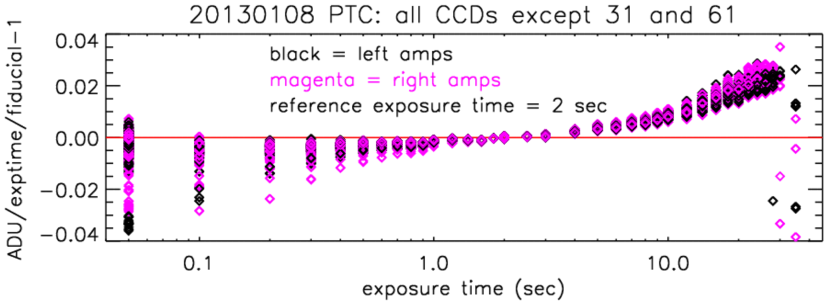
Figure 1: Nonlinearities of 120 DECam amplifiers. The mean signal level of the dome flat (after correction for lamp drift) is plotted against exposure time. The $y$ axis plots the fractional change in ADU per second relative to exposures at $T=2$ s—perfectly linear devices would yield zeros. At high light levels, all amplifiers show mild nonlinearity before the onset of saturation. At low light levels, some amplifiers show signal deficits.

The DECam results in Figure 1 show two classes of nonlinearity before the onset of saturation. All devices show a high-light-level nonlinearity consistent with a quadratic response term. A subset of devices show poorly understood nonlinear behavior at very low illumination levels in which some of the first few tens of electrons “disappear.” One amplifier (#31B) shows unstable nonlinearity and is masked from all images as unsuitable for quantitative analyses. The worst remaining amplifier “loses” $\approx 20e$ of charge. The $\mbox{${\bf Nonlin}$}^{-1}$ function does linearize this response, though one should be cautious about precision photometry at background levels below a few hundred $e$ because the effect is poorly understood.

3.2 Crosstalk

Crosstalk is nominally a linear leakage from “source” amplifier to “victim” channel, and hence there are $140^{2}$ leakage coefficients to determine, since leakage may occur between any of the channels being read out synchronously with the valid science channels (including 5 non-science-quality amplifiers and 16 focus/alignment channels). Each coefficient was evaluated by plotting the median victim amplifier output vs source amplifier signal for a large number of sky images. Fortunately only a handful of inter-CCD amplifiers show detectable ($\gtrsim 10^{-5}$) crosstalk, and always at $<2\times 10^{-4}$ level.

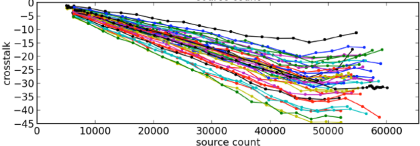
Figure 2: Crosstalk between intra-CCD amplifier pairs. The median “victim” signal is plotted vs source signal for pixel pairs in several hundred low-background sky exposures. Below the source saturation level, crosstalk is linear with coefficient $\leq 10^{-3}$. Nonlinear behavior is apparent when source amplifiers enter their saturation regimes.

Figure 2 shows the victim vs. source trends for all of the intra-CCD amplifier pairs, which have crosstalk coefficients up to $10^{-3}$. It is seen that the crosstalk becomes nonlinear when the source amplifier exceeds its saturation level. These nonlinearities are tabulated and incorporated into the ${\bf XTalk}^{-1}$ operator. Nonlinearity is not significant for the already-small inter-CCD crosstalk.

3.3 Gain and brighter-fatter parameters

The model for the brighter-fatter effect, the determination of its parameters, and the correction algorithm are fully described in Gruen et al. (2015). To summarize: the left, right, top, and bottom ($d\in\{L,R,T,B\}$) edges of pixel $ij$ on the detector are shifted outwards by a distance determined by the charges $q$ in neighboring pixels:

$$\Delta^{d}_{ij}=\sum_{mn}a^{d}_{mn}q_{i+m,j+n}.$$ (27)

The charge in pixel $ij$ is altered as

$$q_{ij}\rightarrow q_{ij}+\Delta^{T}_{ij}\frac{q_{ij}+q_{i,j+1}}{2}+\Delta^{B}_{ij}\frac{q_{ij}+q_{i,j-1}}{2}+\Delta^{L}_{ij}\frac{q_{ij}+q_{i-1,j}}{2}+\Delta^{R}_{ij}\frac{q_{ij}+q_{i+1,j}}{2}.$$ (28)

As the $a$ coefficients are small, the effect can be reversed to good approximation by simply changing the $+$ signs in (28) to minus signs. The correction is fast to calculate since each $\Delta$ array is a convolution of the Charge image with the kernel(s) $a_{mn}$. The convolution is executed by fast Fourier transform; then the charge shifting is a straightforward vector operation on the pixels.

The $a$ coefficients are the parameters of the model. These are determined by measuring the covariance induced by the brighter-fatter effect between the noise on nearby pixels of dome-flat images. These covariances are measured to high precision from 1200 $r$-band dome flats taken over a full season. The covariances (and the $a$ coefficients derived from them) are observed to be constant in time and identical for the A and B amplifiers on a given CCD, as expected for an effect deriving from properties of the wafer and the gate structures.

Another manifestation of the brighter-fatter effect is the suppression of variance in dome flat images. This invalidates the usual method of determining the amplifier $\mathit{Gain}$, which is to note that the noise variance $V$ expected for a pixel with expectation value $\mu$ (measured in ADU² and ADU, respectively) should be the sum of Poisson noise and read noise:

$$V=\frac{\mu}{\mathit{G}ain}+({\rm RN})^{2}.$$ (29)

$\mathit{Gain}$ is typically determined by regressing $V$ against $\mu$ for a series of dome flats of varying exposure time. The brighter-fatter effect, however, introduces a term $\sim a\mu^{2}$ into this equation. The gain is over-estimated if the data are fit without this term—by 5–10% in the case of DECam CCDs. We determine a single gain per amplifier by a fit that includes the brighter-fatter effect.

3.4 Reference flat

We choose to factor the reference flat image as

$$\mbox{${\bf r}$}(t)=\mbox{${\bf Dome}$}\times\mbox{${\bf SFlat}$}\times\mbox{${\bf GRC}$}(t).$$ (30)

The star flat ${\bf SFlat}$ is a parametric function of array coordinates that serves to correct the errors in the dome flat. ${\bf SFlat}$ is held constant for a given filter and observing epoch. The time dependence of $\mbox{${\bf r}$}(t)$ within an epoch is captured by the global relative calibration function $\mbox{${\bf GRC}$}(t)$, that is nearly constant across the field of view but can vary for each exposure, correcting for atmospheric extinction, mirror-coating aging, etc. There are many fewer parameters in ${\bf SFlat}$ and ${\bf GRC}$ than there are pixels in the array, and we can solve for these parameters using purely internal constraints.

3.4.1 Dome flat usage

We have noted that the ${\bf Dome}$ image is a poor approximation to the response $\mbox{${\bf r}$}(t)$ of the array to focused light from a source with the reference spectrum, since it confuses pixel-area variation and scattered light with the desired measure of response to focused light. Not surprisingly, the best way to calibrate the camera’s response to focused starlight is to measure focused starlight, not diffuse light. Early recognition of this principle led to scanning a single source across the (small) arrays of the time (McLeod et al., 1995; Manfroid, 1995), but we can solve for $\mbox{${\bf r}$}(t)$ much more efficiently using the many sources detected by wide-field arrays. If a population of objects with the reference spectrum were spread across the sky, we could determine the reference flat empirically by finding a model of $\mbox{${\bf r}$}(t)$ that produces uniform fluxes for all exposures of a given reference source. The DES photometric calibration relies primarily upon this internal calibration method (dubbed “ubercalibration” by Padmanabhan et al. (2008)). Note that the internal calibration does not actually require us to know either the reference source spectrum $F_{\rm ref}(\lambda)$ or the reference bandpass $r_{\rm ref}(\lambda)$ in order to determine $\mbox{${\bf r}$}(t)$, nor does it offer information on either.

The success of this method depends upon choosing an observation sequence that can constrain, without degeneracy, a model for $\mbox{${\bf r}$}(t)$ that adequately describes its variations. Unfortunately the stellar data in DES are insufficient to estimate ${\bf r}$ at all 500 million DECam pixels, never mind to do so along with time dependence. Even with a huge number of stellar measurements, the fact that stellar images span several pixels precludes the use of stellar data to map response down to single-pixel scales. Therefore we choose to rely on the dome flats to provide small-scale response information for which a parametric form is not readily constructed.

When the small-scale dome flat variations are truly QE effects, this is a good idea, such as for the “spots” visible in Figure 3. But it is detrimental in that pixel-to-pixel variations in subtended sky area, due to imperfections in the CCD lithography, are mistakenly interpreted as QE variations. The latter probably lead to $\approx 1$ mas RMS astrometric errors for DECam. It may in fact be more accurate to replace the ${\bf Dome}$ factor in Equation (30) with a constant or future cameras, these small-scale variations should be determined by laboratory characterization of the devices before deployment (e.g. Baumer & Roodman, 2015, for LSST).

3.4.2 Star flats

The choices of ${\bf SFlat}$ parameterizations, and the assignment of parameters, are described in detail in Bernstein et al. (2017b). We give a short summary here.

The ${\bf SFlat}$ parameterization is expressed as a sum of terms in magnitude space, i.e. multiplicative in $\mbox{${\bf r}$}.$ We begin with independent polynomial variation across each CCD in the mosaic, which essentially replace the large-scale behavior of ${\bf Dome}$ with patterns constrained by stellar data. The ${\bf SFlat}$ model also includes terms to compensate for known pixel-area variations at the edges of the devices (“glowing edges”) and in annular patterns related to inhomogeneities in the silicon wafers (“tree rings”) (Plazas et al., 2014).

The parameters of ${\bf SFlat}$ are chosen to optimize internal agreement of stellar photometry in a series of $\approx 20$ exposures targeted on a rich star field. The exposures are dithered with spacings from 10″ up to the 1° radius of the DECam field, to generate constraints on ${\bf SFlat}$ across this range of spatial scales, using several $\times 10^{5}$ stellar measurements per filter. These “star flat” sequences are taken in each filter every few months during bright time. The ${\bf SFlat}$ for the star flat sequence is taken as the instrumental response for the observing epoch. For processing of the star flat sequences, we model $\mbox{${\bf GRC}$}(t)$ with a single free extinction constant per exposure.

The internal calibration procedure can, if applied to all stars within the well-behaved range of color $p$, also derive the spatial and temporal variation of the color term $\mbox{${\bf c}$}(t)$. As with the reference flat ${\bf r}$, the color term is modeled with a static function of array coordinates, plus a per-exposure term $c_{G}(t)$ that is constant across the array. All stars in the well-behaved range are used to constrain ${\bf SFlat}$ and ${\bf c}$ simultaneously.

The images are first flattened using ${\bf Dome}$, and fluxes for each star are extracted using aperture photometry. The flux $f_{\alpha t}$ of star $\alpha$ in image $t$ is converted to $m_{\alpha t}=m_{0}-2.5\log_{10}f_{\alpha t}$ with some nominal zeropoint $m_{0}$. If $\sigma_{\alpha t}$ is the measurement uncertainty on $m_{\alpha t}$, then we seek to minimize

$$\chi^{2}=\sum_{\alpha}\sum_{t}\frac{\left[m_{\alpha t}-S({\bf x}_{\alpha,t})-p_{\alpha}c({\bf x}_{\alpha t})-G(t)-p_{\alpha}c_{G}(t)-m_{\alpha}\right]^{2}}{\sigma_{\alpha t}^{2}}.$$ (31)

We define $S=-2.5\log_{10}\mbox{${\bf SFlat}$},$ and likewise the scalars $G(t)$ and $c_{G}(t)$ are the logarithms of ${\bf GRC}$ and a color term for each exposure. The observed pixel positions ${\bf x}_{\alpha t}$ and color $p_{\alpha}$ of star $\alpha$ are known, and its true magnitude $m_{\alpha}$ is a free parameter. There are $O(10^{3})$ free parameters in the $S$ and $c$ functions and the $G$ and $c_{G}$ values.

Figure 3 shows the dome flat, star flat, and their product, the reference flat, for one of the DECam filters in one of the observing epochs. The second row of the Figure indicates that the effects measured by the star flat—scattered light, pixel-area variations, and color mismatches between dome lamps and stars—are generally smooth across the array and dominated by a scattered light “doughnut” with a peak-to-peak amplitude of 4%. The structure remaining in the reference flat is dominated by variations in QE from CCD to CCD, with $<0.01$ mag variation within each device. The zoomed images show that most of the “tree-ring” pattern in the domes is suppressed by the star flat, as expected from pixel-size fluctuations, although we do not understand why the tree rings still remain to some extent in the reference flat. The corner “tape bump” features that remain in the reference flat are known to be from pixel-size variations, but our star flat parametric models do not have enough freedom to constrain or remove these from the reference flat. We currently have no means to determine whether the remaining fine-scale features in the reference flat are from QE variations or pixel-size variations, though we suspect primarily the latter.

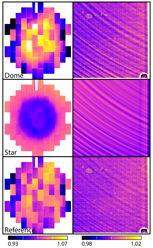
Figure 3: The top row shows a dome flat from DECam through the $z$ filter. At left is a view of the entire focal plane, and at right is 1000-pixel-wide region in the corner of CCD S31 (a.k.a. CCD3). The middle row shows the parametric star flat image derived for this filter, and at bottom is their product, which is our best estimate of the response to focused starlight. In principle the star flat detects and removes structures in the dome flat due to pixel-size variation, scattered light, and color differences between the dome LEDs and stars, leaving only true efficiency variations in the reference flat. On large scales, the star flat removes a scattered-light “doughnut” and the reference flat is very smooth except for CCD-to-CCD variations in QE. On small scales there remain features we believe are pixel-area variation, but our parametric star flat models do not have the freedom to remove them properly. See section 3.4 for details.

The optimized $\chi^{2}$ value is invariant under the transformations $G\rightarrow G+G_{0},$ $c_{G}\rightarrow c_{G}+c_{0}$, and $m_{\alpha}\rightarrow m_{\alpha}+G_{0}+p_{\alpha}c_{0},$ reflecting our inability to determine the absolute magnitude or color scale with purely internal calibrations. External absolute calibrators are needed to set the flux and color scales. There are other degeneracies in the internal calibration process; further details on the derivation of star flats are in Bernstein et al. (2017b).

3.4.3 Global relative calibration and spectral response function

The above processing of specialized “star flat” observation sequences determines the ${\bf SFlat}$ vector for a given epoch and filter. When multiplied by the dome, it yields the ${\bf r}$ which homogenizes the measurements of stellar fluxes across the array at the time the star flat data were acquired. In the DES pipeline, this ${\bf r}$ is used to flatten all images obtained during the epoch, and stellar fluxes are derived from these images.

The next step is to derive the global relative calibration function $\mbox{${\bf GRC}$}(t)$ which can be applied to these cataloged fluxes to homogenize fluxes over all $t$, insuring that a given star would yield the same measured flux when placed at any surveyed sky location at any time during the survey. Starting with Y3A1 reductions, this is done for DES survey exposures by the forward global calibration module (FGCM), described in Burke et al. (2017), which in fact yields a model for the chromatic response function $\mbox{${\bf r}$}(\lambda,t)$ by combining a static model of the telescope/camera spectral response with a time-varying model of the atmospheric transmission $S_{\rm atm}(\lambda,t)$. The atmospheric transmission is in turn modelled with nightly values for the parameters for the major atmospheric optical processes: absorption by water vapor, ozone, and well-mixed molecules; plus Rayleigh scattering and aerosol scattering.

The atmospheric modelling is attempted only for cloudless nights. For data taken through clouds, $\mbox{${\bf GRC}$}(t)$ is derived by finding a distinct zeropoint shift and color term that bring each CCD of each exposure into agreement with overlapping exposures taken on clear nights. This procedure can benefit from the on-site thermal-infrared all-sky imager RASICAM (Reil et al., 2014), which definitively indicates which nights are free of clouds.

As proposed by Stubbs & Tonry (2006), FGCM splits the system spectroscopic response into an atmospheric part (anything outside the dome) and an instrumental function. The atmospheric portion is taken as constant across the field on clear nights and the instrumental function is assumed constant for a given filter during an observing epoch. Both functions are characterized using a mix of auxiliary instrumentation and internal calibrations.

The instrumental response is measured by the DECal narrowband flat-field illumination system (Marshall et al., 2016). DECal directs the output of a monochromator to the dome flat screen via optical fibers and a projector system, which are designed to ensure that the illumination pattern is independent of wavelength. Furthermore the pupil is close to uniform. A calibrated photodiode at the top ring of the telescope measures the brightness of dome illumination as the monochromator is swept across each filter.

Let $\mbox{${\bf DECal}$}(\lambda)$ be the DECam output divided by the photodiode signal, so it gives the response to diffuse light at the top ring. If we multiply this by the atmospheric transmission $S_{\rm atm}(\lambda,t)$, we should obtain the response of the instrument to celestial diffuse light. Because the DECal illuminators do not fill the telescope pupil in the exact same way as the night sky does, the DECal signals differs from the celestial one by a spatial function D. Specializing Equation (16) to a monochromatic source spectrum, and inserting the atmospheric transmission to get the total system response, we get

$$S_{\rm atm}(\lambda,t)\mbox{${\bf DECal}$}(\lambda) \propto r_{\rm ref}(\lambda)\mbox{${\bf r}$}(\lambda,t)\left[1+\mbox{${\bf s_{\rm bg}}$}(\lambda)\right]\times\mbox{\boldmath$\Omega$}\times{\bf D}$$ (32)

$$\Rightarrow\quad r_{\rm ref}(\lambda)\mbox{${\bf r}$}(\lambda,t) \propto S_{\rm atm}(\lambda,t)\times\frac{\mbox{${\bf DECal}$}(\lambda)}{\left[1+\mbox{${\bf s_{\rm bg}}$}(\lambda)\right]\times\mbox{\boldmath$\Omega$}\times{\bf D}}.$$ (33)

DECal is designed to have wavelength dependence of D be small, as is that of $\Omega$. If we ignore the wavelength dependence of the scattered-light fraction $\mbox{${\bf s_{\rm bg}}$}(\lambda)$ across the band of each filter, then the product of ${\bf DECal}$ and $S_{\rm atm}$ give the spectral response $\mbox{${\bf r}$}(\lambda,t)$ up to some time-independent function of pixels. The unknown function is determined by the star-flat measurement of $\mbox{${\bf r}$}(t).$

The scattered-light function $\mbox{${\bf s_{\rm bg}}$}(\lambda)$ is problematic as we have no means to distinguish scattered from focused light in the DECal flats. And unfortunately there is reason to suspect that it does vary within a band: stray light from filter reflections requires (at least) one transmission and one reflection by the filter, so scales as $T(1-T)$ if $T$ is the filter transmission. This signal should peak dramatically as DECal scans across the filter shoulders. In the future we may be able to model this effect and refine the instrument spectral models. Since the transition from 10% to 90% of peak transmission occurs within $\leq 12\%$ of the bandwidth for each DES filter, we do not expect wavelength of variation of $\mbox{${\bf s_{\rm bg}}$}(\lambda)$ to be significantly altering the color corrections, which are already small.

The nightly parameters of the atmospheric transmission $S_{\rm atm}(\lambda,t)$ are constrained by forcing agreement on magnitudes and colors between observations taken on different nights. The atmospheric constituents are further constrained by external data: The barometric pressure and airmass for every observation are recorded and determine the optical depths of the well-mixed molecular components. Synthetic photometry indicates that ozone variations will contribute less than 1 mmag to $\mbox{${\bf C}$}(t;p)$ in the DECam bands, and hence a typical value is assumed for all observations (Li et al., 2016). The ATMCam instrument (Li et al., 2014) continuously monitors a bright star through four narrow filters selected to constrain the remaining aerosol and water vapor components. The latter is also monitored by continuously by a high-precision GPS receiver. These instruments (which are not always in service) are supplemented by internal color constraints to estimate the remaining atmospheric values for each night.

With the ${\bf DECal}$ scans and the nightly atmospheric model in hand, we can integrate any source-spectrum family to derive the spectral flux correction factor $\mbox{${\bf C}$}(\lambda,t;p)$. Recall that the star flat process yields an empirical color term $\mbox{${\bf c}$}(t)$ for stellar spectra. Stellar spectra are well known and hence ${\bf c}$ is a known special case of $\mbox{${\bf C}$}(t;p)$, hence ${\bf c}$ is a consistency check. For example, DECal scans detect a 6 nm center-to-edge change in the blue cutoff of the DES $i$-band filter (Marshall et al., 2016). Synthetic stellar photometry predicts a radial color term that agrees to better than 1 mmag with the values empirically measured from the star flats (Li et al., 2016).

3.5 Absolute calibration

The absolute flux scale $f_{1}$ of the DES natural system in each filter is determined through observations of spectrophotometric standard stars. Current estimates of $f_{1}$ are made using the HST CalSpec standard star C26202, which lies in one of the DES supernova fields (which are observed $\approx$weekly) and is within the dynamic range of our imaging. A sample of DA white dwarf stars in the DES footprint is being measured and modelled for use as absolute calibrators. A more thorough treatment will be presented in a later publication.

3.6 Background templates

The background subtraction technique requires derivation of the component templates $\mbox{${\bf Sky}$}_{k}.$ This is done through a principal-components analysis (PCA) of $\approx 1000$ images taken in a given filter in a given observing epoch. Appendix A describes this procedure.

Figure 4: The first four principal components of the background in the DECam $z$ filter. At the top are subsampled views of the full focal plane, and at bottom are closeups of one of the edge CCDs (S31$=$CCD 3). The first PC (essentially the median sky signal) shows structure on large scales, because the scattered-light doughnut has a different brightness for night-sky illumination than from the dome-flat illumination. The small-scale structure is fringing. The second and third PC’s are nearly pure orthogonal linear gradients with no fringing. The fourth PC has doughnut and fringe structure, consistent with a physical origin in the variation of the ratio of airglow to moonlight.

Figure 4 plots the four sky templates derived for the $z$ band. Here it is apparent that the dominant template (essentially the median sky signal) contains signatures of fringing as well as the scattered-light “doughnut,” and a color difference from the dome flat. Weaker components capture gradients in the sky illumination, and changes in the ratio of airglow to continuum background.

3.7 Astrometric calibration

Determination of the map $(x,y,t)\leftrightarrow(\theta,\phi)$ between pixel and sky coordinates is accomplished by an internal-calibration procedure nearly completely analogous to the photometric methods, using the same star-flat exposure sequences. Degeneracies in the internal calibration are resolved by including stellar positions from the Gaia DR1 catalog in the analysis (Gaia Collaboration, 2016). The full DECam astrometric model and its derivation are described in Bernstein et al. (2017a).

3.8 Bad pixel mask

For each epoch a static bad pixel mask (BPM) is created by noting pixels in the array which have unusually high, low, or noisy levels in the bias and/or dome flat exposures. We also mask the 15 pixels closest to each edge of each CCD, because distortions of the electric field near the device edges cause changes in pixel effective area that are too large, and potentially background-dependent, to be correctable to the desired science accuracy. Pixels with any of these flags set are ignored in all processing.

The BPM additionally flags as “suspect” some other array regions that are useful for most analyses, but have subtle quirks that preclude calibration to the same accuracy as the bulk of the array. The suspect regions include the areas 16–30 pixels from the detector edge; the “tape bump” features on the CCD that have small but highly structured pixel-size variations; and some regions that acquire excess noise when transferring through traps or hot pixels on their way to the readout amplifier. Suspect pixels are detrended and carried through to final images in the normal way, but the flag persists so that the most precise analyses (e.g. weak gravitational lensing, parallax, and proper motion) can ignore these data. Morganson et al. (2017) document the BPM flags and the mask generating process in more detail.

4 The detrending and calibration pipeline

The DES “Final Cut” pipeline takes the ${\bf Raw}$ images from the camera and produces an estimate of the ${\bf Fluence}$ images by inverting the photons-to-ADU model described in Section 2. The output product is a FITS-format file for each CCD containing three images: the ${\bf Science}$ image containing the ${\bf Fluence}$ estimate; a ${\bf Mask}$ bitmap image annotating the reliability of each pixel’s fluence; and a ${\bf Weight}$ image giving the inverse of the noise variance of the pixel excluding the Poisson noise from any astronomical sources in the pixel. In this section we enumerate the operations on these three images that comprise the pipeline. This section provides a mathematical description of the pipeline operations; an operational description is in Morganson et al. (2017).

1. Bias and crosstalk removal: A ${\bf Science}$ image is first created for each CCD by subtracting overscan and bias in the standard way, and applying the crosstalk correction to each set of simultaneously-read pixels:

   $$\mbox{${\bf Science}$}(t)={\bf XTalk}^{-1}\left[\mbox{${\bf Raw}$}(t)-{\bf Overscan}(t)-{\bf Zero}\right].$$ (34)

2. Linearization and gain: The linearization function and gain for each amplifier are applied next:

   $$\mbox{${\bf Science}$}(t)\leftarrow\mbox{${\bf Nonlin}$}^{-1}\left[\mbox{${\bf Science}$}(t)\right]\times\mbox{${\bf Gain}$}.$$ (35)

   At this point, as per Equation (26), the ${\bf Science}$ image should equal the ${\bf Charge}$ image containing the number of photoelectrons collected in each pixel.

3. Defect masking: Some pixels will be known at this point to have inaccurate charge measures. A ${\bf Mask}$ bitmask image is created by combining the pixel defects held in the BPM file with an additional saturation flag set for all pixels whose charge exceeds the saturation level measured for their output amplifier. Morganson et al. (2017) provide a full listing of the mask bits and their meanings.

4. Brighter/fatter correction: The operation

   $$\mbox{${\bf Science}$}(t)\leftarrow{\rm BF}^{-1}\left[\mbox{${\bf Science}$}(t)\right]$$ (36)

   is applied using the model described in section 3.3. The ${\bf Science}$ image now should reflect the number of photoelectrons created, rather than collected, in each pixel. This is equivalent to the ${\bf Rate}$ image, except that we do not divide the ${\bf Science}$ image by the exposure time $T$.

5. Dome flattening: We execute

   $$\mbox{${\bf Science}$}(t)\leftarrow\frac{\mbox{${\bf Science}$}(t)}{\mbox{${\bf Dome}$}}$$ (37)

   at this point, in other words we apply just one of the factors in the reference image defined by Equation (30). None of the processing depends upon this being done, but applying an approximate multiplicative correction makes it easier to inspect the images and identify subtle signals and defects without being visually overwhelmed by flat-field features.

6. Sky subtraction: The coefficients $b_{tk}$ of the background templates $\mbox{${\bf Sky}$}_{k}$ are determined as described in Section A.3, and the background-subtraction operation consists of subtracting the scaled templates:

   $$\mbox{${\bf Science}$}(t)\leftarrow{\bf H}\left[\mbox{${\bf Science}$}(t)\right]=\mbox{${\bf Science}$}(t)-\sum_{k}b_{tk}\mbox{${\bf Sky}$}_{k}.$$ (38)

   The sky templates are constructed from dome-flattened images and hence already have the dome response divided out.

7. Weight creation: Once we have a background estimate we can create the weight image as the inverse of the sum of Poisson and read noise:

   $$\mbox{${\bf Weight}$}(t)=\frac{\mbox{${\bf Dome}$}^{2}}{\mbox{${\bf Dome}$}\times\sum_{k}b_{tk}{\bf Sky}_{k}+{\bf RN}^{2}},$$ (39)

   where RN is the read noise (in electrons). The ${\bf Dome}$ terms appear because the image is no longer quite in units of electrons after the earlier step of dome flattening.

   Note that we include variance from shot noise of the background, but do not include shot noise in the source photons. Analysis programs are responsible for adding the source noise term.

8. Star flattening: With the background now near zero, we apply the next term in the reference flat from Equation (30):

   $$\mbox{${\bf Science}$}(t) \leftarrow\frac{\mbox{${\bf Science}$}(t)}{\mbox{${\bf SFlat}$}}$$ (40)

   $$\mbox{${\bf Weight}$}(t) \leftarrow\mbox{${\bf Weight}$}(t)\times\mbox{${\bf SFlat}$}^{2}.$$ (41)

   This is the output image that is saved to the DES archive. It is not quite equal to the $\mbox{${\bf Fluence}$}(t)$ image that gives fluxes in the reference system - the $\mbox{${\bf GRC}$}(t)$ factor from Equation (30) is missing. $\mbox{${\bf GRC}$}(t)$ are applied to the cataloged fluxes, not to the image pixels themselves. This is a practical consideration: we need to produce the catalog in order to derive the global relative calibration solutions. It is faster to rescale the catalog by ${\bf GRC}$ than to re-scale the images and re-extract the sources.

9. Contaminant masking: Pattern-recognition algorithms are run on ${\bf Science}$ to identify pixels that do not represent celestial fluxes; appropriate bits are set in the ${\bf Mask}$ image.

   • The TRAIL bit is set for CCD bleed trails.

   • The STAR bit is set for a circular region around each very bright star, extending to the radius where the stellar halo fades back to the sky level and will not interfere with identification of faint sources.

   • The EDGEBLEED bit indicates a condition peculiar to the DECam CCDs: if a bright bleed trail reaches the serial register, charge flows along rows and obliterates a large region abutting the serial register for that amplifier. An example is shown in Figure 5.

     

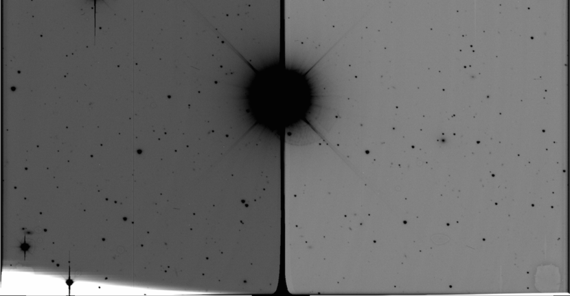
     Figure 5: An “edge bleed” on CCD N29 of exposure 233392, in which a bleeding column from a very bright star reaches the serial register, spreads horizontally, and perturbs the signal chain for up to an entire row’s worth of readouts after the bleed trail. This bleed trail happens to straddle the split between the two output amplifiers.

   • The CRAY bit is set where cosmic rays are detected.

   • The STREAK bit is set where meteor, asteroid, or airplane trails are detected.

   The algorithms for identifying these features are described in Morganson et al. (2017).

10. Cataloging: The ${\bf Science}$ image is analyzed using the SExtractor code (Bertin & Arnouts, 1996), which produces a catalog containing fluxes, positions, and other measurements of each detected source. The details of our use of SExtractor are in Morganson et al. (2017). Information from the ${\bf Mask}$ and ${\bf Weight}$ images are also passed to SExtractor so that it can calculate uncertainties and appropriately flag objects containing invalid or suspect pixels. This catalog and the images then become the basis of DES science analyses. The weak gravitational lensing pipeline, for example, returns to the ${\bf Science}$ images to perform more exacting measures of galaxy shapes than SExtractor does.

11. Global calibration: The cataloged fluxes of high-$S/N$ stellar sources are fed to the global relative calibration algorithms (Burke et al., 2017) to derive the functions $\mbox{${\bf GRC}$}(t)$ (including color terms) that homogenize the full survey magnitudes. As the survey progresses we will recalculate the global solution multiple times with multiple methods. Methods used in previous DES processings/releases are described in Tucker et al. (2007) and Drlica-Wagner et al. (2017). When objects are retrieved from the catalog database, their fluxes/magnitudes can be adjusted using a chosen global solution. Chromatic corrections can be tabulated given an estimate of the source spectral shape $F_{\star}(\lambda),$ or approximated using the source color and the linearized color corrections $\mbox{${\bf c}$}(t)$.

12. Astrometric calibration: The final astrometric calibration, like the global photometric solution, is done at catalog level. The parameters of the global astrometric solution(s) are used to register the images for co-addition as well as for science analyses. Good solutions are derived using scamp, and more detailed solutions (including chromatic terms) are available from the methods described in Bernstein et al. (2017a).

13. Absolute calibration: An overall magnitude zeropoint determination will be the last step in the calibration process. This requires reduction of exposures targeted on spectrophotometric standards, which then must be tied into the global relative calibration of the survey. The resultant magnitude zeropoint from such an analysis can be applied to the full catalog by the object database. Interim zeropoints are in use from synthetic photometry of the HST CalSpec star C26202.

5 Conclusion

We have provided a coherent mathematical model for the output images of DECam in terms of the astronomical brightness distribution, and a series of algorithms to invert the process to determinations of object fluxes. This careful audit shows that dome flats alone are insufficient to determine the response of the array to stars of a given flux: we use on-sky observations of stellar sources to infer “star flat” corrections for scattered light and pixel-area variations in the dome flats. These corrections exceed 0.04 mag for DECam. Bernstein et al. (2017b) demonstrate that these procedures homogenize the photometry to $\approx 2$ mmag accuracy across time periods of hours, We also present a PCA-based method for removing zodiacal light, airglow, and atmospheric scattered light signals from the images. Pixel-area variations and fringing are among the effects that can impart small-scale structure on the detector output from these “backgrounds,” even though they are highly uniform on the sky. This confounds morphological algorithms for distinguishing background from astrophysical signals of interest. Our algorithm instead relies on the repeatability of the background signals to distinguish them.

There are several subtleties in the interpretation of astronomical images from DECam (and other imagers) that one must attend to for precision analyses:

• Are the values in the images representing the fluence in the pixels (total incident photons), or the mean surface brightness in the image? These differ by a factor of pixel area. Aperture magnitude measurements (summations) assume the former, while model-fitting measurements usually assume the latter. The DESDM pipeline produces fluence images.

• The pixel centers do not form a square grid on the sky when pixel areas vary. Model-fitting algorithms and morphological measures must be aware of this even if the images are in surface-brightness normalization.

• The response $\mbox{${\bf r}$}(\lambda,t)$ of the instrument to focused light depends on array position, wavelength, and time. In producing a single calibrated output image for an exposure, we need to designate some nominal source spectral shape $F_{\rm ref}(\lambda)$ to define the reference flat field $\mbox{${\bf r}$}(t)$ that is applied to exposure $t$. The image is only homogeneously calibrated for sources with this spectrum; a position- and time-dependent correction must be applied to homogenize the calibration for sources with different spectral shape. The DES catalogs now model and tabulate these chromatic corrections.

• The PCA sky subtraction algorithm only attempts to remove light from near-Lambertian background sources that repeat in every exposure with only a few degrees of freedom—namely airglow, zodiacal light, and atmospheric scattered light. Episodic contaminants such as stray reflections from bright stars are identified with different algorithms. Downstream codes must make the division between background and signal for diffuse sources such as Galactic dust reflection or intra-cluster light.

• Likewise the weight maps in DESDM outputs present the (inverse) variance only from backgrounds and read noise. The contributions from shot noise in sources should be estimated from a source model, not from the counts in the image.

The model and inversion algorithms we construct for DECam should be generally applicable to wide-field astronomical imagers. Indeed there are commonalities between the DES pipeline and those being used for other current wide-field CCD surveys such as PanSTARRS1 (Magnier et al., 2016), the Kilo-Degree Survey (de Jong et al., 2015), and the Hyper-Suprime Cam survey (Aihara et al., 2017). DECam can be calibrated very reliably (as quantified in other papers) because the optics and detector are very stable and well-behaved. The detectors have very little “personality,” with only mild non-linearities and no known significant hysteresis. The edge bleed phenomenon is the only substantial quirk that affects our high-background exposures. The calibration images, gains, etc., are found to be stable for months at a time, urthermore DECam is on the equatorially mounted Blanco telescope, thus the camera and telescope form a rigid unit. Newer telescopes are exclusively alt-az mounts, so there is continuous rotation between telescope and camera, which may substantially complicate the behavior of the calibrations.

The code implementing these detrending algorithms is all publicly available as part of the DESDM software repository. Most of the detrending steps (2–8 in Section 4), as well as the derivation of the PCA sky templates, are implemented in the pixcorrect Python package and would require minimal alteration, if any, for use on data not adhering to DECam formats. All detrending steps are efficiently implemented as numpy array operations.

Appendix A Principle-component sky subtraction

We start from the assumption in Equation (22) that any given count-rate image $\mbox{${\bf Rate}$}(t)$ is the sum of a sparse component (the astrophysical sources of interest), a zero-mean noise component, and a background component that is a linear function of a small number $K$ of sky “templates.” For this Appendix we will use the notation that ${\bf R}_{t},{\bf S}_{t},$ and ${\bf N}_{t}$ are the count rate, sparse (object) component, and noise components of exposure $t$, expressed as vectors over the $N_{\rm pix}$ pixel positions. We define matrices $R,S,$ and $N$ such that element $t,i$ of each is the value at pixel $i$ in exposure $1\leq t\leq N_{\rm exp}$. We thus seek the $N_{\rm pix}\times K$ matrix $V$ of sky template vectors and the $N_{\rm exp}\times K$ matrix $U$ of coefficients per exposure such that

$$R=S+UV^{T}+N.$$ (A1)

This “robust principle components” problem is common, e.g. in computer vision applications, and the subject of much algorithm development (Candès et al., 2011). But it is quite unmanageable in its native form, since the matrix $R$ is of dimensions $\approx 10^{3}\times 10^{9}$ for the set of exposures from which we wish to build the template set. We will therefore create a decimation operator $D$ which compresses an image vector ${\bf R}$ to a feature vector $\tilde{\bf R}$ of length $N_{f}\ll N_{\rm pix}.$ We will choose $D$ to be linear in the sense that

$$D(a_{1}{\bf R}_{1}+a_{2}{\bf R}_{2})=a_{1}D({\bf R_{1}})+a_{2}D({\bf R}_{2}),$$ (A2)

and that it does not destroy the sparsity, i.e. $\tilde{\bf S}=D({\bf S})$ is also a sparse in the sense of having the majority of its elements be free of source flux. In this case, we can apply $D$ to each row (image) of the $R,N,V,$ and $S$ matrices and transform (A1) to

$$\tilde{R}=\tilde{S}+U\tilde{V}^{T}+\tilde{N},$$ (A3)

with the $U$ vector conserved. As long as $D({\bf V}_{k})\neq 0,$ meaning that the decimation does not project away (or greatly attenuate) the signal of background template ${\bf V}_{k},$ we can as a first step solve for $U$ on the reduced-size problem (A3). Then in step (2), we can obtain the full-resolution templates $V$ with a column-by-column solution to Equation (A1). Step (3) will be to derive coefficients $u_{k}$ to apply to an arbitrary new image ${\bf R}$ that was not part of the $N_{\rm exp}$ images used to construct the templates.

A.1 Deriving coefficients $U$

Our operator $D$ should yield a decimated $\tilde{\bf R}$ which is altered by all of the physical parameters expected to alter the background. We expect changes in the large-scale pattern of focused and scattered background light to arise from changes in lunar phase and the positions of the sun, moon, and telescope. We divide the image into $N_{D}\times N_{D}$ pixel subarrays, and produce as $\tilde{\bf R}$ the medians of each subarray. Typically we take $N_{D}=128.$ The resultant “mini-sky” image is not only smaller, but has greatly reduced noise and is more sparse than the original image. Objects smaller than $N_{D}$ pixels are filtered away by the median, and large disturbances to the background (such as ghosts of bright stars, reflection nebulae, or intra-cluster light) occupy the same fraction of the compressed image’s pixels as in the original.

A concern is that airglow fringing, one of the most important backgrounds to remove, will be largely suppressed by the median at scale $N_{D},$ such that PCA of $\tilde{R}$ cannot recover the elements of $U$ that depend on the strength and excitation state of the airglow. We therefore take an $8\times 8$ block median of one of the CCDs (which still resolves the fringes), and append to the data vector $\tilde{\bf R}$ a $2\times 2$ subsampling of this image. The final feature vector $\tilde{R}$ has $N_{f}\approx 10^{4.5}$ elements and the linear algebra operations are much faster than the disk access times for the exposures.

With a compressed $\tilde{R}$ that should manifest all changes to the background, we proceed to execute a robust PCA decomposition via the following algorithm:

1. Begin a rank-one approximation of $\tilde{R}\approx{\bf u}{\bf v}^{T}$ with vectors ${\bf u}$ and ${\bf v}$ by initializing $v_{k}=1.$

2. Set $u_{t}=\textrm{median}_{i}(\tilde{R}_{ti}/v_{i}).$

3. Set $v_{i}=\textrm{median}_{t}(\tilde{R}_{ti}/u_{t}).$ Iterate with step 2 to convergence of ${\bf u}$ and ${\bf v}.$

4. Rescale $\tilde{R}_{ti}\leftarrow\tilde{R}_{ti}/(u_{t}v_{i})$ so all elements are near unity.

5. Conduct a standard PCA of $\tilde{R}$ and retain the $N_{\rm keep}\sim 20$ most significant components in a trial decomposition $\tilde{R}\approx U\tilde{V}^{T}.$

6. For each exposure $t$, define $\sigma_{t}$ as the RMS value of the residual mini-image $\tilde{\bf R}_{t}-\sum_{k}U_{tk}\tilde{\bf V}_{k}.$

7. For some chosen $\sigma$-clipping threshold $g$, replace all pixels having residual $>g\sigma$ with the value of the rank-$N_{\rm keep}$ approximation. This step excludes super-pixels that remain contaminated by sources and ghosts. Exposures with very large $\sigma$ are discarded from the process as ill-described by the low-rank decomposition.

8. Iterate to step 5 until $U$ converges, typically 3–4 iterations.

9. Rescale $U$ and $\tilde{V}$ with ${\bf u}$ and ${\bf v}$ to make them represent the low-rank decomposition of the original $\tilde{R}$ matrix. We further rescale $U$ and $\tilde{V}$ such that the elements of each row of $\tilde{V}$ (which are decimated sky templates) has RMS value of unity. The $U_{tk}$ elements then give the typical amplitude (in count rate) of the contribution of template $k$ to the background of exposure $t$.

10. Select the number $K$ of templates to retain in the sky model by noting where the amplitudes $U_{tk}$ of the corresponding corrections become insignificant.

A.2 Deriving full-resolution templates $V$

With $U$ in hand, Equation (A1) separates into an independent robust linear regression for each pixel $i$ with unknowns $V_{ki}$:

$$R_{ti}=S_{ti}+\sum_{k=1}^{K}U_{tk}V_{ki}+N_{ti}.$$ (A4)

We solve this system for each $i$ using a standard linear regression with aggressive $\sigma$-clipping of outliers, since we expect a substantial fraction of the $N_{\rm exp}\approx 10^{3}$ samples at this pixel to be “contaminated” by object flux. This is the most time consuming portion of the analysis since there are $5\times 10^{8}$ such solutions to execute per DECam filter. But this operation is trivially parallelized and the computation time is insignificant compared to the DESDM pipeline execution time.

A.3 Fitting coefficients to exposures

Once the sky template matrix $V$ is known for a given filter during a given epoch, we can execute the sky subtraction on any exposure’s data ${\bf R}_{t},$ whether or not it was among the $N_{\rm exp}$ used to derive the templates. This is again a robust linear regression operation, which we conduct on a decimated version of the exposure using the decimated templates $\tilde{V}$:

$$\left[D({\bf R}_{t})\right]_{i}=\tilde{S}_{t}+\sum_{k=1}^{K}u_{tk}\tilde{V}_{ik}+\tilde{N}_{ti}.$$ (A5)

We solve for the $K$ coefficients $u_{tk}$ which best satisfy this equation, once again using a $\sigma$-clipping iteration to exclude super-pixels that are perturbed by large-scale objects or image artifacts.

This fit to the mini-sky image yields valuable diagnostic information as well as the background coefficients $u_{tk}$: the fraction $f_{\rm clip}$ of super-pixels that were clipped away; the RMS variation $\sigma$ of those super-pixels that remained; and the residual of the mini-sky image to the best sky model. A high $f_{\rm clip}$ usually indicates the presence of a large spurious-light source in the image, such as an airplane trail, or ghosts of a bright star. A high $\sigma$ value indicates an aberrant background pattern, such as can occur for images taken through patchy clouds, or with a very bright, nearby moon. These artifacts are readily identified by visual inspection of the mini-sky residuals.

A.4 Results for DECam

For DECam, we find that $>99\%$ of the background signal is described as a linear combination of $K\leq 4$ sky components (except for exposures taken through patchy clouds). Figure 4 shows the first four principle components of background in the DECam $z$ filter. The top row shows the “mini-sky” decimated images for each component row of $\tilde{V}$. The second row shows a closeup of a single CCD to reveal the presence of fringing signals in the full-resolution $V$. All of the signals here are shown relative to the dome flat pattern.

The dominant PC1 is basically the median night-sky signal. The upper left panel reveals that the background signal differs from the dome flat in several respects: first, there is a significant slope, suggesting that there is a gradient in the dome illumination system; second, the donut structure suggests that the scattered light amplitude differs between dome and sky illumination; and we also see CCD-to-CCD step functions, which are likely due to a spectral differences between dome and night sky combined with varying spectral response of the CCDs. The lower left panel reveals the fringing signal, which we expect to be present in the night sky but not in the domes. In the bluer filters there is less fringe signal, but one can see in the sky templates other small-scale deviations between dome and sky signals, which are likely attributable to color differences. A morphology-based sky subtraction would fail to identify such issues.

In all the filters we find that PC2 and PC3 are essentially two orthogonal linear slopes of sky flux across the array. These are readily associated with gradients in brightness expected across the FOV as the distance to the moon or sun varies, or gradients in the zodiacal brightness. Note there are no fringes visible in PC2 or PC3: the airglow is not involved in these gradients. PC2 and PC3 coefficients are found to be usefully diagnostic of problems such as the occultation of the telescope beam by the observatory dome.

Fringes reappear in PC4 for $z$ band, as does a donut pattern. Our hypothesis is that PC4 is generated by a change in the ratio of airglow intensity to the intensity of backgrounds that have nearly-solar continuum spectra (twilight, moonlight, and zodiacal light). PC4 basically allows the fringe amplitude to vary independently of the large-scale patterns, but we see from the upper-right panel that this is accompanied by a change in the overall illumination pattern. Apparently the airglow/solar ratio change is manifested as an overall color shift of the night sky as well as in the fringing patterns. In fact we have found the large-scale sky pattern is fully predictive of the fringe amplitude for this filter: we recover the fringe pattern in PC4 even if we omit from our decimation operator $D$ the secondary small-scale feature vector described above. In practice, therefore, we have found the DECam PCA can be conducted just with the $128\times 128$ median-filtered “mini-sky” images.

Principal components at $k>4$ are found to contain smooth quadratic and increasingly higher-order polynomial variation across the focal plane, with no visible fringe or small-scale components. As such patterns are at most a few $e$ amplitude in normal images, and are getting into the realm where they may be excited by astrophysical sources such as reflection nebulae or bright star ghosts, we truncate our templates at $K=4$ and leave higher-order sky variation to the sky subtraction algorithm executed at the cataloging step.

In the $g,r,$ and $i$ bands the fringes are nearly absent, but other small-scale structures (such as tree rings) are visible in PC1. The DECam detectors have low fringe amplitudes because their thick, deep-depletion bulk and good anti-reflection coatings yield high quantum efficiency to the silicon bandgap cutoff. This makes them weak Fabry-Perot resonators for the airglow lines. Other detectors with stronger fringe patterns may benefit even more than DECam from this PCA-based sky subtraction technique, because their fringe patterns will be stronger and may also exhibit detectable pattern shifts as excitation conditions of the ionospheric radicals change.

References

- Aihara et al. (2017) Aihara, H. et al. 2017, arxiv:1702.08449
- Antilogus et al. (2014) Antilogus, P., Astier, P., Doherty, P., Guyonnet, A., & Regnault, N. 2014, Journal of Instrumentation, 9, C03048
- Baumer & Roodman (2015) Baumer, M. A., & Roodman, A. 2015, Journal of Instrumentation, 10, C05024
- Bernstein et al. (2017a) Bernstein, G. M., Armstrong, R., Plazas, A. A., et al. 2017, PASP, 129, 074503
- Bernstein et al. (2017b) Bernstein, G. M. et al. 2017, in preparation
- Bertin (2006) Bertin, E. 2006, Astronomical Data Analysis Software and Systems XV, 351, 112
- Bertin & Arnouts (1996) Bertin, E., & Arnouts, S. 1996, A&AS, 117, 393
- Burke et al. (2015) Burke, D. L. et al. (2015), AJ, 147, 19
- Burke et al. (2017) Burke, E. et al. (2017), arxiv:1706.01542
- Candès et al. (2011) Candès, E. J., Li, X., Ma, Y., & Wright, J. 2011, Journal of the ACM, 58, 11
- de Jong et al. (2015) de Jong, J. T. A., Verdoes Kleijn, G. A., Boxhoorn, D. R., et al. 2015, A&A, 582, A62
- The Dark Energy Survey Collaboration (2005) The Dark Energy Survey Collaboration 2005, arXiv:astro-ph/0510346
- Desai et al. (2012) Desai, S., Armstrong, R., Mohr, J. J., et al. 2012, ApJ, 757, 83
- Drlica-Wagner et al. (2017) Drlica-Wagner, A. et al. (2017), DES Y1A1 Gold Catalog, (in prep.)
- Flaugher et al. (2015) Flaugher, B., Diehl, H. T., Honscheid, K., et al. 2015, AJ, 150, 150
- Gaia Collaboration (2016) The Gaia Collaboration 2016, A&A, 595, A2
- Gruen et al. (2015) Gruen, D., Bernstein, G. M., Jarvis, M., et al. 2015, Journal of Instrumentation, 10, C05032
- Gunn & Westphal (1981) Gunn, J. E., & Westphal, J. A. 1981, Proc. SPIE, 290, 16
- Gunn (2014) Gunn, J. 2014, Journal of Instrumentation, 9, C04021
- Jacoby et al. (1998) Jacoby, G. H., Liang, M., Vaughnn, D., Reed, R., & Armandroff, T. 1998, Proc. SPIE, 3355, 721
- Laher et al. (2014) Laher, R. R., Surace, J., Grillmair, C. J., et al. 2014, PASP, 126, 674
- Li et al. (2014) Li, T., DePoy, D. L., Marshall, J. L., et al. 2014, Proc. SPIE, 9147, 91476Z
- Li et al. (2016) Li, T. S., DePoy, D. L., Marshall, J. L., et al. 2016, AJ, 151, 157
- Magnier et al. (2016) Magnier, E. A. et al. 2016, arXiv:1612.05242
- Manfroid (1995) Manfroid, J. 1995, A&AS, 113, 587
- Marshall et al. (2016) Marshall, J. L., Rheault, J.-P., DePoy, D. L., et al. 2016, The Science of Calibration, 503, 49
- McLeod et al. (1995) McLeod, B. A., Bernstein, G. M., Rieke, M. J., Tollestrup, E. V., & Fazio, G. G. 1995, ApJS, 96, 117
- Mohr et al. (2012) Mohr, J. J., Armstrong, R., Bertin, E., et al. 2012, Proc. SPIE, 8451, 84510D
- Morganson et al. (2017) Morganson, E. et al. (2017), DESDM paper (in prep.)
- Padmanabhan et al. (2008) Padmanabhan, N., Schlegel, D. J., Finkbeiner, D. P., et al. 2008, ApJ, 674, 1217-1233
- Plazas et al. (2014) Plazas, A. A., Bernstein, G. M., & Sheldon, E. S. 2014, PASP, 126, 750
- Reil et al. (2014) Reil, K., Lewis, P., Schindler, R., & Zhang, Z. 2014, Proc. SPIE, 9149, 91490U
- Schirmer (2013) Schirmer, M. 2013, ApJS, 209, 21
- Sevilla et al. (2011) Sevilla, I., Armstrong, R., Bertin, E., et al. 2011, arXiv:1109.6741
- Stubbs & Tonry (2006) Stubbs, C. W., & Tonry, J. L. 2006, ApJ, 646, 1436
- Tucker et al. (2007) Tucker, D. L., Annis, J. T., Lin, H., et al. 2007, ASPC, 364, 187
- Tyson (1986) Tyson, J. A. 1986, Journal of the Optical Society of America A, 3, 2131
- Tyson (2015) Tyson, J. A. 2015, Journal of Instrumentation, 10, C05022