The Cardassian expansion revisited: constraints from updated Hubble parameter measurements and Type Ia Supernovae data

Abstract

Motivated by an updated compilation of observational Hubble data (OHD) which consist of 51 points in the redshift range $0.07<z<2.36$, we study an interesting model known as Cardassian which drives the late cosmic acceleration without a dark energy component. Our compilation contains 31 data points measured with the differential age method by Jimenez & Loeb (2002), and 20 data points obtained from clustering of galaxies. We focus on two modified Friedmann equations: the original Cardassian (OC) expansion and the modified polytropic Cardassian (MPC). The dimensionless Hubble, $E(z)$, and the deceleration parameter, $q(z)$, are revisited in order to constrain the OC and MPC free parameters, first with the OHD and then contrasted with recent observations of SN Ia using the compressed and full joint-light-analysis (JLA) samples. We also perform a joint analysis using the combination OHD plus compressed JLA. Our results show that the OC and MPC models are in agreement with the standard cosmology and naturally introduce a cosmological-constant-like extra term in the canonical Friedmann equation with the capability of accelerating the Universe without dark energy.

1 Introduction

The cold dark matter with a cosmological constant ($\Lambda$CDM) model is the cornerstone of modern cosmology. It has shown an unprecedented success predicting and reproducing the dynamics and evolution of the Universe. $\Lambda$CDM is based on two important but unknown components, dark matter (DM) and dark energy (DE), which constitute $\sim 96\%$ of the total content of our Universe (Ade et al., 2016). In this standard paradigm, the DE, responsible of the late cosmic acceleration, is supplied by a cosmological constant (CC), which is associated to vacuum energy. Although several cosmological observations favor the CC, some theoretical problems arise when we try a renormalization of the quantum vacuum fluctuations using an appropriate cut-off at the Planck energy. However, the problem becomes insurmountable, giving a difference of $\sim 120$ orders in magnitude between theory and observations (Weinberg, 1989; Zeldovich, 1968). In addition, the problem of coincidence, i.e. the similitude between the energy density of matter and dark energy at the present epoch, remains as an open question (Weinberg, 1989; Zeldovich, 1968).

To overcome these problems, several alternatives to the CC are proposed, such as quintessence, phantom energy, Chaplygin gas, holographic DE, Galileons, among others (see Copeland et al., 2006; Carroll, 2001, for a complete review). Geometrical approaches are also used to explain the DE dynamics (i.e. brane theories) like Dvali, Gabadaze and Porrati (DGP, Deffayet et al., 2002), Randall-Sundrum I and II (RSI,RSII, Randall & Sundrum, 1999a, b) or $f(R)$ theories (Buchdahl, 1970; Starobinsky, 1980; Cembranos, 2009); each one having important pros and cons.

An interesting alternative, closely related to geometrical models, is the Cardassian expansion model for which there is no DE and the late cosmic acceleration is driven by the modification of the Friedmann equation as $H^{2}=f(\rho)$ (Xu, 2012), where $f(\rho)$ is a functional form of the energy density of the Universe. Freese & Lewis (2002) proposed $f(\rho)\propto\rho+\rho^{n}$ in order to obtain a late acceleration stage under certain conditions on the $n$ parameter, naming the model as the Cardassian expansion (hereafter the original Cardassian, OC, model). However, this expression can be naturally deduced from extra dimensional theories (DGP, RSI, RSII, etc.), which imprint the effects of a 5D space-time (the bulk) in our 4D space-time (the brane) at cosmological scales. In the case of the DGP model, a consequence of this kind of geometry is a density parameter that evolves as $(\sqrt{\rho+\alpha}+\beta)^{2}$, where $\alpha$ and $\beta$ are constants related to the threshold between the brane and the bulk, allowing an accelerated epoch driven only by geometry. In the case of RS models, a quadratic term in the energy momentum tensor modifies the right-hand-side of the Friedmann equation as $a\rho+b\rho^{2}$ (Shiromizu et al., 2000), with a correspondence to the Cardassian models when $n=2$. Thus, the topological structure of the brane and the bulk can naturally produce the Cardassian Friedmann equation. Indeed, it is possible to obtain a $n$-energy-momentum tensor from a Gauss equation with a product of $n$-extrinsic curvatures, which leads to the $\rho^{n}$ extra term in the Friedmann equation of the original Cardassian model. Therefore, the model motivation is based on extra dimensions arising from a fundamental theory (for an excellent review of extra dimensions models, see for instance Maartens, 2004, or Maartens 2000 for a cosmological point of view). Another alternative interpretation is to consider a fluid (that may or may not be in an intrinsically four-dimensional metric) with an extra contribution to the energy-momentum tensor (Gondolo & Freese, 2003). Both interpretations are interesting and the standard cosmological dynamics can be mimicked without the need to postulate a dark energy component . In addition, we notice that it is possible to recover a CC when $\rho^{n}\to 1$, without adding it by hand. An OC model generalization can be obtained by considering an additional exponent in the right-hand-side of the Friedmann equation as $f(\rho)\propto\rho(1+\rho^{l(n-1)})^{1/l}$ which is called modified polytropic Cardassian (hereafter MPC) model by analogy with a fluid interpretation (Gondolo & Freese, 2002).

The Cardassian models are extensively studied in the literature. They have been tested with several cosmological observations (see for example Wang et al., 2003; Wei et al., 2015; Liang et al., 2011; Feng & Li, 2010; Xu, 2012; Li et al., 2012, and references therein). Wei et al. (2015) put constraints on the OC model parameters using a joint analysis of gamma ray burst data and Type Ia supernovae (SN Ia) of the Union 2.1 sample (Suzuki et al., 2012). Recently, Magaña et al. (2015) used the strong lensing measurements in the galaxy cluster Abell 1689, baryon acoustic oscillations (BAO), cosmic microwave background (CMB) data from nine-year Wilkinson microwave anisotropy probe (WMAP) observations (Hinshaw et al., 2013), and the SN Ia LOSS sample (Ganeshalingam et al., 2013) to constrain the MPC parameters.

In this work, we revisit the Cardassian expansion models with an universe that contains baryons, DM, together with the radiation component. We explore two functional forms of the Friedmann equation: one with the OC parameter $n$ (following Freese & Lewis, 2002), and the other one considering also the $l$ exponent (following Gondolo & Freese, 2003). These Cardassian models are tested using an update sample of observational Hubble parameter data (OHD) and the compressed joint-light-analysis (cJLA) SN Ia data by Betoule et al. (2014).

As a final comment, while we were finalizing this paper, an arxiv submitted article (Ref. Zhai et al., 2017a) addressed a similar revision of the Cardassian models. While the main focus of Ref. Zhai et al. (2017a) is to match the the Cardassian Friedmann equations to $f(T,\mathcal{T})$ theory through the action principle, our work focus on providing bounds to the Cardassian models using OHD (see also Zhai et al., 2017b). Nonetheless, the authors also provide constraints derived from SN Ia, BAO, and CMB data.

The paper is organized as follows. In Sec. 2 the Cardassian cosmology is revisited, introducing two proposals for the Friedmann equation, which correspond to the OC and MPC models, and the deceleration parameter is calculated. In Sec. 3, we present the data and methodology in order to study the Cardassian models using OHD and SN Ia observations. In Sec. 4, we show the constraints for the free parameters presenting the novel contrast with the updated sample. Finally, Sec. 5 presents our conclusions and the possible outlooks into future studies.

We will henceforth use units in which $c=\hbar=1$ (unless explicitly written).

2 The Cardassian Cosmology

2.1 Original Cardassian model

The original Cardassian model was introduced by Freese & Lewis (2002) to explain the accelerated expansion of the Universe without DE. Motivated by braneworld theory, this model modifies the Friedmann equation as

$$H^{2}=\frac{8\pi G\rho_{t}}{3}+B\rho_{t}^{n},$$ (1)

where $H=\dot{a}/a$ is the Hubble parameter, $a$ is the scale factor of the Universe, $G$ is the Newtonian gravitational constant, $B$ is a dimensional coupling constant that depends on the theory, and the total matter density is $\rho_{t}=\rho_{m}+\rho_{r}$. The recent Planck measurements (Ade et al., 2014; Ade et al., 2016) suggest a curvature energy density $\Omega_{k}\simeq 0$, thus we assume a flat geometry. The conservation equation is maintained in the traditional form:

$$\dot{\rho}+3H(\rho+p)=0.$$ (2)

The matter density (dark matter and baryons), $\rho_{m}=\rho_{m0}a^{-3}$, and the radiation density, $\rho_{r}=\rho_{r0}a^{-4}$, evolution can be computed from Eq. (2). The second term in the right hand side of Eq. (1), known as the Cardassian term, drives the universe to an accelerated phase if the exponent $n$ satisfies $n<2/3$. At early times, this corrective term is negligible and the dynamics of the universe is governed by the canonical term of the Friedmann equation. When the universe evolves, the traditional energy density and the one due to the Cardassian correction becomes equal at redshift $z_{Card}\sim\mathcal{O}(1)$. Later on, the Cardassian term begins to dominate the evolution of the universe and source the cosmic acceleration. The Eq. (1) reproduces the $\Lambda$CDM model for $n=0$. As in the standard case, it is possible to define a new critical density for the OC model, $\rho_{Nc}$, which satisfies the Eq. (1) and can be written as $\rho_{Nc}=\rho_{c}F(B,n)$, where $\rho_{c}=3H^{2}/8\pi G$ is the standard critical density, and $F(B,n)$ is a function which depends on the OC parameters and the components of the Universe.

The Raychaudhuri equation can be written in the form:

$$\frac{\ddot{a}}{a}=-\frac{4\pi G}{3}(\rho_{t}+3p_{t})-B\left[\left(\frac{3n}{2}-1\right)\rho_{t}^{n}+\frac{3}{2}n\rho_{t}^{n-1}p_{t}\right],$$ (3)

where Eqs. (1) and (2) were used. From Eq. (1), it is possible to obtain the dimensionless Hubble parameter $E^{2}(z)\equiv H^{2}(z)/H^{2}_{0}$ as,

$$E(z,\mathbf{\Theta})^{2}=\Omega_{\mathrm{std}}+(1-\Omega_{m0}-\Omega_{r0})\left[\frac{\Omega_{\mathrm{std}}}{\Omega_{m0}+\Omega_{r0}}\right]^{n},$$ (4)

where $\mathbf{\Theta}=(\Omega_{m0},h,n)$ is the free parameter vector to be constrained by the data, $\Omega_{r0}=\rho_{r0}/\rho_{c}$ is the current standard density parameter for the radiation component, $\Omega_{m0}=\rho_{m0}/\rho_{c}$ is the observed standard density parameter for matter (baryons and DM), and we define $\Omega_{\mathrm{std}}\equiv\Omega_{m0}(1+z)^{3}+\Omega_{r0}(1+z)^{4}$. We compute $\Omega_{r0}=2.469\times 10^{-5}h^{-2}(1+0.2271N_{eff})$ (Komatsu et al., 2011), where $N_{eff}=3.04$ is the standard number of relativistic species (Mangano et al., 2002). Notice that we have also imposed a flatness condition on the total content of the Universe (for further details on how to obtain Eq. (4) see Sen & Sen, 2003a, b).

The deceleration parameter, defined as $q\equiv-\ddot{a}/aH^{2}$, can be written as

$$q(z,\mathbf{\Theta})=\frac{\Omega_{\mathrm{std}}-\frac{1}{2}\Omega_{m0}(1+z)^{3}}{E^{2}(z,\mathbf{\Theta})}+\frac{1-\Omega_{m0}-\Omega_{r0}}{(\Omega_{m0}+\Omega_{r0})^{n}}\times$$

$$\left[\left(\frac{3n}{2}-1\right)+\frac{n\Omega_{r0}}{2\Omega_{std}}(1+z)^{4}\right]\frac{\Omega_{\mathrm{std}}^{n}}{E^{2}(z,\mathbf{\Theta})}.$$ (5)

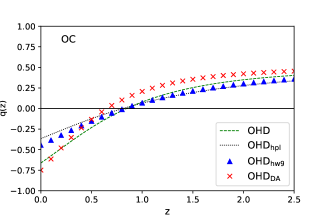
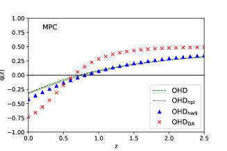
In order to investigate whether the OC model can drive the late cosmic acceleration, it is necessary to reconstruct the $q(z)$ using the mean values for the $\mathbf{\Theta}$ parameters.

2.2 Modified polytropic Cardassian model

Gondolo & Freese (2002, 2003) introduced a simple generalization of the Cardassian model, the modified polytropic Cardassian, by introducing an additional exponent $l$ (see also Wang et al., 2003). The modified Friedmann equation with this generalization can be written as

$$H^{2}=\frac{8\pi G}{3}\rho_{t}\beta^{1/l},$$ (6)

where

$$\beta\equiv 1+\left(\frac{\rho_{Card}}{\rho_{t}}\right)^{l(1-n)},$$ (7)

and $\rho_{Card}$ is the characteristic energy density, with $n<2/3$ and $l>0$. In concordance with the previous Friedmann Eq. (1) and following Ade et al. (2014); Ade et al. (2016), we also assume $\Omega_{k}\simeq 0$. The Eq. (6) reproduce the $\Lambda$CDM model for $l=1$ and $n=0$. Thus, the acceleration equation is

$$\frac{\ddot{a}}{a}=-\frac{4\pi G}{3}\rho_{t}\beta^{1/l}+4\pi G(1-n)\rho_{t}\left(1-\frac{1}{\beta}\right)\beta^{1/l}.$$ (8)

The MPC model (Eq. 9) has been studied by several authors using different data with $\rho_{t}=\rho_{m}$ (see for example Feng & Li, 2010) and also with $\rho_{t}=\rho_{m}+\rho_{r}$ together with a curvature term (Shi et al., 2012). Here we consider a flat MPC with matter and radiation components. After straightforward calculations, the dimensionless $E^{2}(z,\mathbf{\Theta})$ parameter reads as:

$$E^{2}(z,\mathbf{\Theta})=\Omega_{r0}(1+z)^{4}+\Omega_{m0}(1+z)^{3}\beta(z,\mathbf{\Theta})^{1/l},\quad$$ (9)

where

$$\beta(z,\mathbf{\Theta})\equiv 1+\left[\left(\frac{1-\Omega_{r0}}{\Omega_{m0}}\right)^{l}-1\right](1+z)^{3l(n-1)},$$ (10)

being $\mathbf{\Theta}=(\Omega_{m0},h,l,n)$, the free parameter vector to be fitted by the data.

In addition, $q(z,\mathbf{\Theta})$, can be written as

$$q(z,\mathbf{\Theta})=\frac{\Omega_{m0}\beta(z,\mathbf{\Theta})^{1/l}}{2E^{2}(z,\mathbf{\Theta})}\left[1-3(1-n)\left(1-\frac{1}{\beta(z,\mathbf{\Theta})}\right)\right]\times$$

$$(1+z)^{3}+\frac{\Omega_{r0}}{E^{2}(z,\mathbf{\Theta})}(1+z)^{4}.$$ (11)

We use the $\mathbf{\Theta}$ mean values in the last expression to reconstruct the deceleration parameter $q(z)$ and investigate whether the MPC model is consistent with a late cosmic acceleration.

3 Data and Methodology

The OC and MPC model parameters are constrained using an updated OHD sample, which contains $51$ data points, and the compressed SN Ia data set from the JLA full sample by Betoule et al. (2014), which contains $31$ data points. In the following we briefly introduce these data sets.

3.1 Observational Hubble data

The “differential age” (DA) method proposed by Jimenez & Loeb (2002) allows us to measure the expansion rate of the Universe at redshift $z$, i.e. $H(z)$. This technique compares the ages of early-type-galaxies (i.e., without ongoing star formation) with similar metallicity and separated by a small redshift interval (for instance, Moresco et al., 2012, measure $\Delta z\sim 0.04$ at $z<0.4$ and $\Delta z\sim 0.3$ at $z>0.4$). Thus, a $H(z)$ point can be estimated using

$$H(z)=-\frac{1}{1+z}\frac{\mathrm{dz}}{\mathrm{dt}},$$ (12)

where $\mathrm{dz/dt}$ is measured using the $4000\mbox{\AA}$ break ($D4000$) feature as function of redshift. A strong $D4000$ break depends on the metallicity and the age of the stellar population of the early-type galaxy. Thus, the technique by Jimenez & Loeb (2002) offers to directly measure the Hubble parameter using spectroscopic dating of passively-evolving galaxy to compare their ages and metallicities, providing $H(z)$ measurements that are model-independent. These H(z) points are given by different authors as Zhang et al. (2014); Moresco et al. (2012); Moresco (2015); Moresco et al. (2016); Stern et al. (2010), and constitute the majority of our sample (31 points). In addition, we use 20 points from BAO measurements, although some of them being correlated because they either belong to the same analysis or there is overlapping among the galaxy samples, through this work, we assume that they are independent measurements. Moreover, some data points are biased because they are estimated using a sound horizon, $r_{d}$, at the drag epoch, $z_{d}$, which depends on the cosmological model (Melia & López-Corredoira, 2017). Points provided by different authors use different values for the $r_{d}$ in clustering measurements, for instance Anderson et al. (2014) take $153.19$ Mpc while Gaztanaga et al. (2009) choose $153.3$ Mpc, etc.

Table 1 shows an updated compilation of OHD accumulating a total of 51 points (other recent compilations are provided by Farooq et al., 2017; Zhang & Xia, 2016; Yu & Wang, 2016). We have included all the points of the previous references, although priority has been given to the measurements that comes from the DA method and have also been measured with clustering at the same redshift. As reference to compare our results, we also give the data point by Riess et al. (2016b) who measured a Hubble constant $H_{0}$ with $2.4\%$ of uncertainty. Authors argue that this improvement is due to a better calibration (using Cepheids) of the distance to 11 SN Ia host galaxies, reducing the error by almost one percent. We use this sample to constrain the free parameters of the OC and MPC models and look for an alternative solution to the accelerated expansion of the Universe. The figure-of-merit for the OHD is given by

$$\chi_{\mbox{OHD}}^{2}=\sum_{i=1}^{N_{OHD}}\frac{\left[H(z_{i})-H_{obs}(z_{i})\right]^{2}}{\sigma_{H_{i}}^{2}},$$ (13)

where $N_{OHD}$ is the number of the observational Hubble parameter $H_{obs}(z_{i})$ at $z_{i}$, $\sigma_{H_{i}}$ is its error, and $H(z_{i})$ is the theoretical value for a given model.

$z$	$H(z)$	$\sigma_{H}$	Reference	Method
	$\mbox{km\,s}^{-1}\mbox{Mpc}^{-1}$	kms-1Mpc-1
0	73.24	1.74	Riess et al. (2016b)	SN Ia/Cepheid
0.07	69	19.6	Zhang et al. (2014)	DA
0.1	69	12	Stern et al. (2010)	DA
0.12	68.6	26.2	Zhang et al. (2014)	DA
0.17	83	8	Stern et al. (2010)	DA
0.1791	75	4	Moresco et al. (2012)	DA
0.1993	75	5	Moresco et al. (2012)	DA
0.2	72.9	29.6	Zhang et al. (2014)	DA
0.24	79.69	2.65	Gaztanaga et al. (2009)	Clustering
0.27	77	14	Stern et al. (2010)	DA
0.28	88.8	36.6	Zhang et al. (2014)	DA
0.3	81.7	6.22	Oka et al. (2014)	Clustering
0.31	78.17	4.74	Wang et al. (2017)	Clustering
0.35	82.7	8.4	Chuang & Wang (2013)	Clustering
0.3519	83	14	Moresco et al. (2012)	DA
0.36	79.93	3.39	Wang et al. (2017)	Clustering
0.38	81.5	1.9	Alam et al. (2016)	Clustering
0.3802	83	13.5	Moresco et al. (2016)	DA
0.4	95	17	Stern et al. (2010)	DA
0.4004	77	10.2	Moresco et al. (2016)	DA
0.4247	87.1	11.2	Moresco et al. (2016)	DA
0.43	86.45	3.68	Gaztanaga et al. (2009)	Clustering
0.44	82.6	7.8	Blake et al. (2012)	Clustering
0.4497	92.8	12.9	Moresco et al. (2016)	DA
0.47	89	34	Ratsimbazafy et al. (2017)	DA
0.4783	80.9	9	Moresco et al. (2016)	DA
0.48	97	62	Stern et al. (2010)	DA
0.51	90.4	1.9	Alam et al. (2016)	Clustering
0.52	94.35	2.65	Wang et al. (2017)	Clustering
0.56	93.33	2.32	Wang et al. (2017)	Clustering
0.57	92.9	7.8	Anderson et al. (2014)	Clustering
0.59	98.48	3.19	Wang et al. (2017)	Clustering
0.5929	104	13	Moresco et al. (2012)	DA
0.6	87.9	6.1	Blake et al. (2012)	Clustering
0.61	97.3	2.1	Alam et al. (2016)	Clustering
0.64	98.82	2.99	Wang et al. (2017)	Clustering
0.6797	92	8	Moresco et al. (2012)	DA
0.73	97.3	7	Blake et al. (2012)	Clustering
0.7812	105	12	Moresco et al. (2012)	DA
0.8754	125	17	Moresco et al. (2012)	DA
0.88	90	40	Stern et al. (2010)	DA
0.9	117	23	Stern et al. (2010)	DA
1.037	154	20	Moresco et al. (2012)	DA
1.3	168	17	Stern et al. (2010)	DA
1.363	160	33.6	Moresco (2015)	DA
1.43	177	18	Stern et al. (2010)	DA
1.53	140	14	Stern et al. (2010)	DA
1.75	202	40	Stern et al. (2010)	DA
1.965	186.5	50.4	Moresco (2015)	DA
2.33	224	8	Bautista et al. (2017)	Clustering
2.34	222	7	Delubac et al. (2015)	Clustering
2.36	226	8	Font-Ribera et al. (2014)	Clustering

Table 1: 52 Hubble parameter measurements $H(z)$ (in km s^-1Mpc^-1) and their errors, $\sigma_{H}$, at redshift $z$. The first point is not included in the MCMC analysis, it was only considered as a Gaussian prior in some tests. The method column refers as to how to $H(z)$ was obtained: DA stands for differential age method, and clustering comes from BAO measurements.

3.1.1 An homogeneous OHD sample

As mentioned above, the OHD from clustering (BAO features) are biased due to an underlying $\Lambda$CDM cosmology to estimate $r_{d}$. Different authors used different values in the cosmological parameters and obtained different sound horizons at the drag epoch, which are used to break the degeneracy in $Hr_{d}$. Furthermore, the determination of $H(z)$ from BAO features is computed taking into account very conservative systematic errors (see the discussion by Melia & López-Corredoira, 2017; Leaf & Melia, 2017).

As a first attempt to homogenize and achieve model independence for the OHD obtained from clustering, we take the value $Hr_{d}$ for each data point and assume a common value $r_{d}$ for the entire data set. We consider two $r_{d}$ estimations: $r_{\mathrm{dpl}}=147.33\pm 0.49$ Mpc and $r_{\mathrm{dw9}}=152.3\pm 1.3$ Mpc from the most recent Planck (Ade et al., 2016) and WMAP9 (Bennett et al., 2013) measurements respectively. In addition, we also take into account three other sources of errors that could affect $r_{d}$ due to its contamination by a cosmological model. The first one comes from the error of each reported value. The second error considers the possible range of $r_{d}$ values provided by separate CMB measurements, i.e. the difference between the sound horizon given by WMAP9 and Planck. This error is the one producing the largest impact on the $r_{d}$ mean value (3.37 % and 3.26 % for the Planck and WMAP9 data point respectively). The last error to take into account is the difference between $r_{d}$ used to obtain the OHD and the one that would be obtained if we assume another cosmological model instead of $\Lambda$CDM. Hereafter we use the one obtained for a DE constant equation-of-state ($w$) CDM model, $r_{\mathrm{d\omega cdm}}=148.38$ Mpc (the cosmological parameters for this model are provided by Neveu et al., 2017). Adding in quadrature the percentage for these three errors, we obtain $r_{\mathrm{dpl}}=147.33\pm 5.08$ Mpc and $r_{\mathrm{dw9}}=152.3\pm 6.42$ Mpc. Finally, we propagate this new error to the quantity $H(z)$ to secure a new homogenized and model-independent sample (Table 2).

$z$	$H(z)\pm\sigma_{H}(r_{\mathrm{dpl}})$	$H(z)\pm\sigma_{H}(r_{\mathrm{dw9}})$
	$\mbox{km\,s}^{-1}\mbox{Mpc}^{-1}$	$\mbox{km\,s}^{-1}\mbox{Mpc}^{-1}$
0.24	82.37 $\pm$ 3.94	79.69 $\pm$ 4.28
0.3	78.83 $\pm$ 6.58	76.26 $\pm$ 6.63
0.31	78.39 $\pm$ 5.46	75.83 $\pm$ 5.60
0.35	88.10 $\pm$ 9.45	85.23 $\pm$ 9.37
0.36	80.16 $\pm$ 4.37	77.54 $\pm$ 4.63
0.38	81.74 $\pm$ 3.40	79.08 $\pm$ 3.81
0.43	89.36 $\pm$ 4.89	86.44 $\pm$ 5.18
0.44	85.48 $\pm$ 8.59	82.69 $\pm$ 8.55
0.51	90.67 $\pm$ 3.66	87.71 $\pm$ 4.13
0.52	94.61 $\pm$ 4.20	91.52 $\pm$ 4.63
0.56	93.59 $\pm$ 3.96	90.54 $\pm$ 4.42
0.57	96.59 $\pm$ 8.76	93.44 $\pm$ 8.78
0.59	98.75 $\pm$ 4.66	95.53 $\pm$ 5.07
0.6	90.96 $\pm$ 7.04	87.99 $\pm$ 7.14
0.61	97.59 $\pm$ 3.97	94.41 $\pm$ 4.47
0.64	99.09 $\pm$ 4.53	95.86 $\pm$ 4.97
0.73	100.69 $\pm$ 8.03	97.40 $\pm$ 8.12
2.33	223.99 $\pm$ 11.12	216.69 $\pm$ 11.97
2.34	222.105 $\pm$ 10.38	214.85 $\pm$ 11.31
2.36	226.24 $\pm$ 11.18	218.86 $\pm$ 12.05

Table 2: Homogenized model-independent OHD from clustering (in km s^-1Mpc^-1) and its error, $\sigma_{H}$, at redshift $z$. The first and second columns were obtained using the sound horizon in the drag epoch from Planck and WMAP measurements respectively.

3.2 Type Ia Supernovae (SN Ia)

The SN Ia observations supply the evidence of the accelerated expansion of the Universe. They have been considered a perfect standard candle to measure the geometry and dynamics of the Universe and have been widely used to constrain alternatives cosmological models to explain the late-time cosmic acceleration. Currently, there are several compiled SN Ia samples, for instance, the Union 2.1 compilation by Suzuki et al. (2012) which consists of 580 points in the redshift range $0.015<z<1.41$, and the Lick Observatory Supernova Search (LOSS) sample containing $586$ SN Ia in the redshift range $0.01<z<1.4$ (Ganeshalingam et al., 2013). Recently, Betoule et al. (2014) presented the so-called full JLA (fJLA) sample which contains $740$ points spanning a redshift range $0.01<z<1.2$. The same authors also provide the information of the fJLA data in a compressed set (cJLA) of $31$ binned distance modulus $\mu_{b}$ spanning a redshift range $0.01<z<1.3$, which still remains accurate for some models where the isotropic luminosity distance evolves slightly with redshift. For instance, when the cJLA is used in combination with other cosmological data, the difference between fJLA and cJLA in the mean values for the $w$CDM model parameters is at most $0.018\sigma$. Here we use both, the fJLA and cJLA samples, to constrain the parameters of the OC and MPC models.

3.2.1 Full JLA sample

As mentioned, the full JLA sample contains 740 confirmed SN Ia in the redshift interval $0.01<z<1.2$, which is one of the most recent and reliable SN Ia samples. We use this sample to constrain the parameters of both Cardassian models. The function of merit for the fJLA sample is calculated as:

$$\chi^{2}_{\mbox{fJLA}}=\mathbf{\left(\hat{\mu}-\mu_{Card}\right)^{{\dagger}}\mathrm{C_{\eta}^{-1}}\left(\hat{\mu}-\mu_{Card}\right)},$$ (14)

where $\mu_{Card}=5log_{10}\left(d_{L}/10pc\right)$, and $\mathrm{C_{\eta}}$ is the covariance matrix of $\mathbf{\hat{\mu}}$ provided by Betoule et al. (2014), and is constructed using

$$\mathbf{C_{\eta}} =\left(\mathbf{C_{cal}}+\mathbf{C_{model}}+\mathbf{C_{bias}}+\mathbf{C_{host}}+\mathbf{C_{dust}}\right)$$ (15)

$$+\left(\mathbf{C_{pecvel}}+\mathbf{C_{nonIa}}\right)+\mathbf{C_{stat}},$$

where $\mathbf{C_{cal}},\mathbf{C_{model}},\mathbf{C_{bias}},\mathbf{C_{host}},\mathbf{C_{dust}}$ are systematic uncertainty matrices associated with the calibration, the light curve model, the bias correction, the mass step, and dust uncertainties respectively. $\mathbf{C_{pecvel}}$ and $\mathbf{C_{nonIa}}$ corresponds to systematics uncertainties in the peculiar velocity corrections and the contamination of the Hubble diagram by non-Ia events respectively, $\mathbf{C_{stat}}$ corresponds to an statistical uncertainty obtained from error propagation of the light-curve fit uncertainties. Finally $\hat{\mu}$ is given by

$$\hat{\mu}=m_{b}^{\star}-\left(M_{B}-\alpha\times X_{1}+\beta\times C\right),$$ (16)

where $m_{b}^{\star}$ corresponds to the observed peak magnitude, $\alpha$, $\beta$ and $M_{B}$ are nuisance parameters in the distance estimates. The $X_{1}$ and $C$ variables describe the time stretching of the light-curve and the Supernova color at maximum brightness respectively. The absolute magnitude $M_{B}$ is related to the host stellar mass ($M_{stellar}$) by the step function:

$$M_{B}=\left\{\begin{array}[]{cc}M_{B}^{1}&\hskip 14.22636pt\rm{if}\ M_{stellar}<10^{10}M_{\odot}\ ,\\ M_{B}^{1}+\Delta_{M}&\hskip 14.22636pt\rm{otherwise.}\\ \end{array}\right.$$ (19)

By replacing Eq. (4), Eq. (9), Eq. (15) and Eq. (16) in Eq. (14), we obtain the explicit figure-of-merit $\chi^{2}_{\mathrm{fJLA}}$ for the Cardassian models.

3.2.2 Compressed form of the JLA sample

Table 7 shows the $31$ binned distance modulus at the binned redshift $z_{b}$. The function of merit for the cJLA sample is calculated as:

$$\chi^{2}_{\mbox{cJLA}}=\mathbf{r^{{\dagger}}\mathrm{C_{b}^{-1}}r},$$ (20)

where $\mathrm{C_{b}}$ is the covariance matrix provided by Betoule et al. (2014), and $\mathbf{r}$ is given by

$$\mathbf{r}=\mathbf{\mu_{b}}-M-\log_{10}d_{L}(\mathbf{z_{b}},\mathbf{\Theta}),$$ (21)

where $M$ is a nuisance parameter and $d_{L}$ is the luminosity distance given by

$$d_{L}=(1+z)\frac{c}{H_{0}}\int^{0}_{z}\frac{\mathrm{dz}^{\prime}}{E(z^{\prime},\mathbf{\Theta})}.$$ (22)

By replacing Eq. (4) and Eq. (9) in the last expression, we obtain the explicit figure of merit $\chi^{2}_{\mathrm{cJLA}}$ for the OC and MPC models.

4 Results

A MCMC Bayesian statistical analysis was performed to estimate the ($\Omega_{m0}$,$h$,$n$) and the ($\Omega_{m0}$,$h$,$n$,$l$) parameters for the OC and MPC models respectively. The constructed Gaussian likelihood function for each data set are given by $\mathcal{L}_{\mathrm{OHD}}\propto\exp(-\chi_{\mathrm{OHD}}^{2}/2)$, $\mathcal{L}_{\mathrm{cJLA}}\propto\exp(-\chi_{\mathrm{cJLA}}^{2}/2)$, $\mathcal{L}_{\mathrm{fJLA}}\propto\exp(-\chi_{\mathrm{fJLA}}^{2}/2)$, and $\mathcal{L}_{\mathrm{joint}}\propto\exp(-\chi_{\mathrm{tot}}^{2}/2)$, where $\chi_{\mathrm{tot}}^{2}=\chi_{\mathrm{OHD}}^{2}+\chi_{\mathrm{cJLA}}^{2}$. We use the Affine Invariant Markov chain Monte Carlo (MCMC) Ensemble sampler from the emcee Python module (Foreman-Mackey et al., 2013). In all our computations we consider $3000$ steps to stabilize the estimations (burn-in phase), $6000$ MCMC steps and $1000$ walkers which are initialized in a small ball around the expected points of maximum probability, is estimated with a differential evolution method. For both, OC and MPC models, we assume the following flat priors: $\Omega_{m0}[0,1]$, and $n[-1,2/3]$. For the $l$ MPC parameter we consider the flat prior $[0,6]$. For the $h$ parameter three priors are considered: a flat prior $[0,1]$, and two Gaussian priors, one by Riess et al. (2016b, the first point in Table 1), and the other one by Ade et al. (2016) from Planck 2015 measurements ($h=0.678\pm 0.009$). When the cJLA data are used, we also take a flat prior on the nuisance parameter $M[-1,1]$. The following flat priors $\alpha[0,2]$, $\beta[0,4.0]$, $M^{1}_{B}[-20,-18]$, and $\Delta_{M}[-0.1,0.1]$ are considered when the fJLA sample is employed. To judge the convergence of the sampler, we ask that the acceptance fraction is in the $[0.2-0.5]$ range and check the autocorrelation time which is found to be $\mathcal{O}(60-80)$.

We carry out four runs using different OHD sets: the full observational sample given in Table 1, the $31$ data points obtained using the DA method ($\mathrm{OHD_{DA}}$), and two samples containing the DA points plus those homogenized points from clustering using a common $r_{d}$ estimated from Planck and WMAP measurements (Table 2). We also estimate the OC and MPC parameters using both the cJLA and fJLA samples. Moreover, we perform a joint analysis considering each OHD sample and the cJLA sample. Tables 3 and 4 provide the best fits for the OC and MPC parameters respectively using the different data sets and priors on $h$. Tables 5 and 6 give the constraints from the following joint analysis: OHD+cJLA (J1), $\mathrm{OHD_{DA}}$+cJLA (J2), $\mathrm{OHD_{hpl}}$+CJLA (J3), and $\mathrm{OHD_{hw9}}$+CJLA (J4). We also give the minimum chi-square, $\chi_{min}$, and the reduced $\chi_{red}=\chi_{min}/d.o.f$, where the degree of freedom (d.o.f.) is the difference between the number of data points and the free parameters.

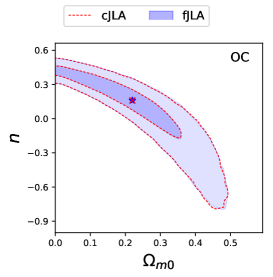
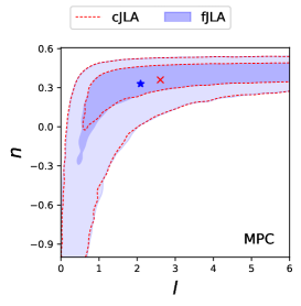
4.1 cJLA vs. fJLA on the Cardassian parameter estimations

The use of the fJLA sample to infer cosmological parameters has a high computational cost when several model are tested. To deal with this, we use the cJLA sample instead of the fJLA. Nevertheless, the former was computed under the standard cosmology. To asses how the Cardassian model constraints are biased when using each SNIa sample, we perform the parameter estimation with different combinations of models, priors, and samples. The several constraints are presented in Tables 3 and 4. Notice that the mean values for the cosmological parameters in the OC model obtained from both SNIa samples are the same. For the MPC model, the largest difference is observed on the $l$ parameter (flat prior on $h$), $\sim 0.18\sigma$. It is smaller for the $n$ parameter when employing a Gaussian prior on $h$. Figure 1 illustrates the comparison of the confidence contours for these parameters using the cJLA and fJLA samples (flat prior on $h$). Figure 2 shows that there is no significant difference in the reconstruction of the $q(z)$ parameter for the OC and MPC models using the constraints obtained from both SNIa samples. Therefore, to optimize the computational time, in the following analysis we only use the compressed JLA sample.

Figure 1: Comparison of the $\Omega_{m0}$-$n$ (top panel) and $n$-$l$ (bottom panel) confidence contours for the OC and MPC parameters within the $1\sigma$ and $3\sigma$ confidence levels using the cJLA (dashed lines) and fJLA (filled and solid lines) samples respectively. In the parameter estimation, a flat prior is considered. The cross and star mark the mean values for each data set.

Figure 2: Reconstruction of the deceleration parameter $q(z)$ for the OC (top panel) and MPC (bottom panel) models using the constraints from the cJLA and fJLA samples when a flat prior on $h$ is considered. Notice that there is no significant differences in the $q(z)$ behavior using each SNIa sample.

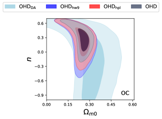
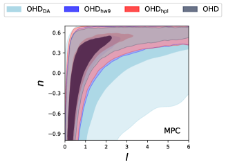
4.2 The effects of the homogeneous OHD subsample in the parameter estimation.

In section §3.1.1, an homogenized and model-independent OHD from clustering was constructed to avoid or reduce biased constraints due to the underlying cosmology or the underestimated systematic errors. Tables 3-4 provide the OC and MPC bounds estimated from the combination of the new computed unbiased OHD from clustering with those obtained from the DA method. The increase on the error of $r_{d}$ also increases the error on $H(z)$, reducing the goodness of the fit ($\chi_{red}$). In spite of this, the advantage of these new limits is that they could be considered unbiased by different cosmological models. Figure 3 shows the contours of the $\Omega_{m0}$-$n$ OC (top panel) and the $n$-$l$ MPC (bottom panel) parameters respectively using the different OHD samples. Note that all the bounds are consistent within the $1\sigma$ and $3\sigma$ C.L. Figure 4 illustrates the $q(z)$ reconstructions using the different OHD data sets. Notice that for the OC model the homogenized OHD samples give slightly different $q(0)$ values than the obtained from the sample in Table 1. For the MPC model, these differences are less significant.

Figure 3: Confidence contours of the $\Omega_{m0}$-$n$ (top panel) and $n$-$l$ (bottom panel) constraints for the OC and MPC models within the $1\sigma$ and $3\sigma$ confidence levels using the OHD sample in Table 1, the OHD_DA data set, and two samples containing the DA points plus those homogenized OHD points from clustering using the $r_{d}$ values from WMAP and Planck measurements. A flat prior on $h$ was considered in the parameter estimation.

Figure 4: Reconstruction of the deceleration parameter $q(z)$ for the OC (top panel) and MPC (bottom panel) models using the constraints from different OHD samples when a flat prior on $h$ is considered.

4.3 The effects of a different Gaussian prior on h.

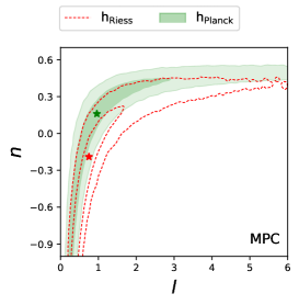
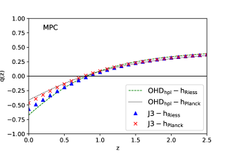
One of the most important problems in cosmology is the tension up to more than $3\sigma$ between the local measurements of the Hubble constant $H_{0}$ and those obtained from the CMB anisotropies (Bernal et al., 2016). The latest estimation by the Planck collaboration (Ade et al., 2016), $h=0.678\pm 0.009$, is in disagreement with the first value given in Table 1. Thus, using different Gaussian priors on $h$ will lead to different constraints on the OC and MPC parameters. Therefore, we carried out all our computations with both priors. Figure 5 illustrates how the confidence contours for the $\Omega_{m0}$-$n$ and $l$-$n$ parameters of the OC (top panel) and MPC (bottom panel) models obtained from OHD_hpl are shifted using each Gaussian prior. Although they are consistent at $3\sigma$, the tension in the constraints is important. In spite of these differences, both results drive the Universe to an accelerated phase but with slightly different transition redshifts (i.e. the redshift at which the Universe passes from a decelerated to an accelerated phase) and amplitude, $q(0)$. In addition, the OC and MPC bounds are consistent with the standard cosmology even when different Gaussian priors are considered.

Figure 5: Comparison of the $\Omega_{m0}$-$n$ (top panel) and $l$-$n$ (bottom panel) confidence contours for the OC and MPC parameters respectively within the $1\sigma$ and $3\sigma$ confidence levels obtained from the OHD_hpl analysis using two Gaussian priors on $h$: $0.732\pm 0.017$ (Riess et al., 2016b) and $0.678\pm 0.009$ (Ade et al., 2016). The stars mark the mean values for each data set.

Figure 6: Reconstruction of the deceleration parameter $q(z)$ for the OC (top panel) and MPC (bottom panel) models using the constraints from the OHD_hpl sample and the joint analysis J3 when a different Gaussian prior on $h$ is considered: $0.732\pm 0.017$ (Riess et al., 2016b) and $0.678\pm 0.009$ (Ade et al., 2016)

4.4 Cosmological implications of the OC and MPC constraints

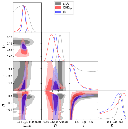
Figure 7b shows the 1D marginalized posterior distributions and the 2D $68\%$, $95\%$, $99\%$ contours for the $\Omega_{m0}$, $h$, and $n$ parameters of the OC model obtained from OHD_hpl, cJLA, and J3 with flat (left panel) and Gaussian (right panel) priors on $h$. Assuming a flat prior on $h$, the $\Omega_{m0}$, $h$ constraints obtained from the different data sets are consistent between them and are in agreement with Planck measurements for the standard model. For the $n$ parameter we found a tension in the constraints obtained from the different data sets. Nevertheless, the bounds have large uncertainties and are consistent among them within the $1\sigma$ CL. Our $n$ constraints are consistent within the $1\sigma$ CL with those estimated by other authors, for instance, $n=-0.04^{+0.07}_{-0.07}$ (Xu, 2012), $n=0.16^{+0.30}_{-0.52}$ (Wei et al., 2015), and $n=-0.022^{+0.05}_{-0.05}$ (Zhai et al., 2017a). It is worth to note that, when the cJLA data are used, $\Omega_{m}$ drop at extremely low values (see the $\Omega_{m0}$-$n$ contour), which is consistent with the results by Wei et al. (2015) who obtained a similar contour using the Union 2.1 data set. In addition, the $\chi_{red}^{2}$ values from the SN Ia data suggest that their errors (cJLA sample) are underestimated.

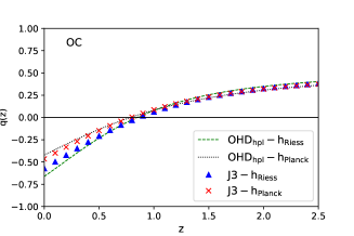
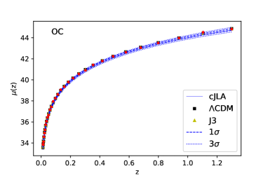
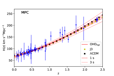
On the other hand, when the Gaussian prior on $h$ by Riess et al. (2016b) is considered, the OHD_hpl provides a better fitting for the OC parameters than those obtained when a flat prior is used (see the $\chi_{red}^{2}$ values). SN Ia data show no important statistical difference in the parameter estimation when flat or Gaussian priors are employed. Notice that we obtain stringent constraints from the joint analysis (see Fig. 7b), which prefers values around $n\sim 0$. Figure 8 shows the fittings to the OHD_hpl (top panel) and cJLA data (bottom panel) using the OHD_hpl, cJLA and J3 constraints for the OC model. A Monte Carlo approach was performed to propagate the error on the $1\sigma$, and $3\sigma$ CL. The comparison between these results and the $\Lambda$CDM fitting reveals that both models are in agreement with the data and there is no significant difference between them. In addition, when the J1, J2, and J4 constraints are used, we found consistent results within the $1\sigma$ confidence level. Therefore, the extra term in the Eq. (1) to the canonical Friedmann equation acts like a CC. However, in the OC models this term can be sourced by an extra dimension instead of the expected vacuum energy.

Table 3: Mean values for the OC parameters ($\Omega_{m0}$, $h$, $n$) derived from OHD and SN Ia data of the cJLA and fJLA sample.

OC model
Parameter	OHD	OHDDA	OHDhpl	OHDhw9	cJLA	fJLA
Flat prior on $h$
$\chi^{2}_{min}$	25.37	15.22	21.25	22.52	32.95	682.28
$\chi^{2}_{red}$	0.52	0.54	0.44	0.46	1.22	0.93
$\Omega_{m0}$	$0.25^{+0.02}_{-0.02}$	$0.30^{+0.06}_{-0.06}$	$0.25^{+0.02}_{-0.03}$	$0.25^{+0.03}_{-0.03}$	$0.22^{+0.11}_{-0.12}$	$0.22^{+0.11}_{-0.12}$
$h$	$0.65^{+0.03}_{-0.03}$	$0.69^{+0.06}_{-0.05}$	$0.66^{+0.04}_{-0.03}$	$0.66^{+0.04}_{-0.03}$	$0.72^{+0.19}_{-0.19}$	$0.72^{+0.18}_{-0.18}$
$n$	$0.26^{+0.16}_{-0.15}$	$-0.19^{+0.51}_{-0.50}$	$0.23^{+0.20}_{-0.20}$	$0.16^{+0.22}_{-0.22}$	$0.16^{+0.17}_{-0.26}$	$0.16^{+0.18}_{-0.26}$
$M(M_{B}^{1})$	–	–	–	–	$0.07^{+0.5}_{-0.66}$	$-18.96^{+0.49}_{-0.64}$
$\Delta_{M}$	–	–	–	–	–	$-0.06^{+0.02}_{-0.01}$
$\alpha$	–	–	–	–	–	$0.14^{+0.006}_{-0.006}$
$\beta$	–	–	–	–	–	$3.10^{+0.08}_{-0.07}$
Gaussian prior on $h=0.732\pm 0.017$
$\chi^{2}_{min}$	28.86	14.47	22.83	23.91	32.95	682.28
$\chi^{2}_{red}$	0.60	0.51	0.47	0.49	1.22	0.93
$\Omega_{m0}$	$0.24^{+0.01}_{-0.01}$	$0.31^{+0.03}_{-0.04}$	$0.24^{+0.01}_{-0.01}$	$0.24^{+0.01}_{-0.01}$	$0.22^{+0.11}_{-0.12}$	$0.22^{+0.11}_{-0.12}$
$h$	$0.71^{+0.01}_{-0.01}$	$0.72^{+0.01}_{-0.01}$	$0.72^{+0.01}_{-0.01}$	$0.72^{+0.01}_{-0.01}$	$0.73^{+0.01}_{-0.01}$	$0.73^{+0.01}_{-0.01}$
$n$	$-0.01^{+0.08}_{-0.08}$	$-0.43^{+0.28}_{-0.30}$	$-0.02^{+0.09}_{-0.10}$	$-0.11^{+0.10}_{-0.11}$	$0.16^{+0.17}_{-0.26}$	$0.16^{+0.18}_{-0.26}$
$M(M_{B}^{1})$	–	–	–	–	$0.10^{+0.05}_{-0.05}$	$-18.94^{+0.05}_{-0.05}$
$\Delta_{M}$	–	–	–	–	–	$-0.06^{+0.02}_{-0.01}$
$\alpha$	–	–	–	–	–	$0.14^{+0.006}_{-0.006}$
$\beta$	–	–	–	–	–	$3.10^{+0.08}_{-0.07}$
Gaussian prior on $h=0.678\pm 0.009$
$\chi^{2}_{min}$	25.24	14.53	20.79	22.04	32.95	–
$\chi^{2}_{red}$	0.52	0.51	0.43	0.45	1.22	–
$\Omega_{m0}$	$0.26^{+0.01}_{-0.01}$	$0.33^{+0.05}_{-0.07}$	$0.26^{+0.02}_{-0.02}$	$0.25^{+0.02}_{-0.02}$	$0.22^{+0.11}_{-0.12}$	–
$h$	$0.67^{+0.008}_{-0.008}$	$0.67^{+0.009}_{-0.009}$	$0.67^{+0.008}_{-0.008}$	$0.67^{+0.008}_{-0.008}$	$0.67^{+0.009}_{-0.009}$	–
$n$	$0.15^{+0.06}_{-0.06}$	$-0.05^{+0.27}_{-0.32}$	$0.17^{+0.08}_{-0.08}$	$0.09^{+0.08}_{-0.09}$	$0.16^{+0.17}_{-0.26}$	–
$M$	–	–	–	–	$-0.06^{+0.03}_{-0.03}$	–

Table 4: Mean values for the MPC parameters ($\Omega_{m0}$, $h$, $n$, $l$) derived from OHD and SN Ia data of the cJLA and fJLA sample.

MPC model
Parameter	OHD	OHDDA	OHDhpl	OHDhw9	cJLA	fJLA
Flat prior on $h$
$\chi^{2}_{min}$	25.31	17.95	21.17	22.98	33.76	682.92
$\chi^{2}_{red}$	0.53	0.66	0.45	0.48	1.29	0.93
$\Omega_{m0}$	$0.25^{+0.04}_{-0.04}$	$0.32^{+0.06}_{-0.07}$	$0.25^{+0.04}_{-0.05}$	$0.25^{+0.04}_{-0.04}$	$0.22^{+0.12}_{-0.13}$	$0.22^{+0.12}_{-0.13}$
$h$	$0.64^{+0.03}_{-0.02}$	$0.68^{+0.07}_{-0.05}$	$0.65^{+0.03}_{-0.03}$	$0.65^{+0.04}_{-0.03}$	$0.72^{+0.18}_{-0.19}$	$0.72^{+0.18}_{-0.18}$
$n$	$0.17^{+0.34}_{-0.68}$	$0.10^{+0.38}_{-0.60}$	$0.25^{+0.29}_{-0.68}$	$0.15^{+0.34}_{-0.65}$	$0.36^{+0.07}_{-0.33}$	$0.33^{+0.09}_{-0.50}$
$l$	$0.77^{+1.45}_{-0.43}$	$2.13^{+2.34}_{-1.33}$	$0.95^{+1.90}_{-0.58}$	$0.92^{+1.66}_{-0.52}$	$2.61^{+2.27}_{-1.83}$	$2.09^{+2.51}_{-1.49}$
$M(M_{B}^{1})$	–	–	–	–	$0.08^{+0.50}_{-0.67}$	$-18.97^{+0.49}_{-0.65}$
$\Delta_{M}$	–	–	–	–	–	$-0.06^{+0.02}_{-0.01}$
$\alpha$	–	–	–	–	–	$0.14^{+0.006}_{-0.006}$
$\beta$	–	–	–	–	–	$3.10^{+0.08}_{-0.07}$
Gaussian prior on $h=0.732\pm 0.017$
$\chi^{2}_{min}$	27.75	14.92	22.40	23.42	33.75	683.17
$\chi^{2}_{red}$	0.59	0.55	0.47	0.49	1.29	0.93
$\Omega_{m0}$	$0.24^{+0.01}_{-0.01}$	$0.32^{+0.03}_{-0.04}$	$0.24^{+0.02}_{-0.02}$	$0.23^{+0.02}_{-0.02}$	$0.22^{+0.12}_{-0.14}$	$0.22^{+0.12}_{-0.13}$
$h$	$0.71^{+0.01}_{-0.01}$	$0.72^{+0.01}_{-0.01}$	$0.72^{+0.01}_{-0.01}$	$0.72^{+0.01}_{-0.01}$	$0.73^{+0.01}_{-0.01}$	$0.73^{+0.01}_{-0.01}$
$n$	$-0.34^{+0.40}_{-0.42}$	$-0.03^{+0.24}_{-0.49}$	$-0.19^{+0.39}_{-0.50}$	$-0.28^{+0.39}_{-0.46}$	$0.36^{+0.07}_{-0.33}$	$0.34^{+0.08}_{-0.47}$
$l$	$0.62^{+0.49}_{-0.20}$	$2.12^{+2.29}_{-1.20}$	$0.75^{+0.80}_{-0.30}$	$0.77^{+0.73}_{-0.28}$	$2.60^{+2.27}_{-1.81}$	$2.26^{+2.44}_{-1.63}$
$M(M_{B}^{1})$	–	–	–	–	$0.10^{+0.05}_{-0.05}$	$-18.94^{+0.05}_{-0.05}$
$\Delta_{M}$	–	–	–	–	–	$-0.06^{+0.02}_{-0.01}$
$\alpha$	–	–	–	–	–	$0.14^{+0.006}_{-0.006}$
$\beta$	–	–	–	–	–	$3.10^{+0.08}_{-0.07}$
Gaussian prior on $h=0.678\pm 0.009$
$\chi^{2}_{min}$	25.03	14.70	20.84	21.96	33.79	–
$\chi^{2}_{red}$	0.53	0.54	0.44	0.46	1.29	–
$\Omega_{m0}$	$0.25^{+0.02}_{-0.02}$	$0.35^{+0.05}_{-0.08}$	$0.26^{+0.03}_{-0.03}$	$0.25^{+0.02}_{-0.03}$	$0.22^{+0.12}_{-0.13}$	–
$h$	$0.67^{+0.008}_{-0.008}$	$0.67^{+0.009}_{-0.009}$	$0.67^{+0.009}_{-0.009}$	$0.67^{+0.009}_{-0.008}$	$0.67^{+0.009}_{-0.009}$	–
$n$	$-0.01^{+0.35}_{-0.57}$	$0.24^{+0.19}_{-0.53}$	$0.16^{+0.26}_{-0.60}$	$0.03^{+0.31}_{-0.58}$	$0.36^{+0.07}_{-0.36}$	–
$l$	$0.71^{+0.95}_{-0.34}$	$2.08^{+2.44}_{-1.37}$	$0.96^{+1.55}_{-0.55}$	$0.87^{+1.22}_{-0.45}$	$2.59^{+2.27}_{-1.8}$	–
$M$	–	–	–	–	$-0.06^{+0.03}_{-0.03}$	–

Table 5: Mean values for the OC parameters ($\Omega_{m0}$, $h$, $n$) derived from a joint analysis OHD$+$cJLA.

OC model
Data set	$\chi^{2}_{min}$	$\chi^{2}_{red}$	$\Omega_{m0}$	$h$	$n$	M
Flat prior on $h$
J1	58.91	$0.71$	$0.25^{+0.01}_{-0.01}$	$0.68^{+0.01}_{-0.01}$	$0.12^{+0.06}_{-0.06}$	$-0.04^{+0.03}_{-0.03}$
J2	48.28	$0.58$	$0.30^{+0.05}_{-0.05}$	$0.68^{+0.02}_{-0.02}$	$-0.001^{+0.15}_{-0.17}$	$-0.03^{+0.06}_{-0.06}$
J3	54.28	$0.66$	$0.25^{+0.02}_{-0.02}$	$0.69^{+0.01}_{-0.01}$	$0.11^{+0.07}_{-0.07}$	$-0.02^{+0.04}_{-0.04}$
J4	55.17	$0.67$	$0.25^{+0.02}_{-0.02}$	$0.67^{+0.01}_{-0.01}$	$0.10^{+0.07}_{-0.08}$	$-0.07^{+0.04}_{-0.04}$
Gaussian prior on $h=0.732\pm 0.017$
J1	63.34	$0.76$	$0.25^{+0.01}_{-0.01}$	$0.70^{+0.01}_{-0.01}$	$0.05^{+0.05}_{-0.05}$	$0.001^{+0.02}_{-0.03}$
J2	50.73	$0.61$	$0.27^{+0.04}_{-0.05}$	$0.71^{+0.01}_{-0.01}$	$0.001^{+0.14}_{-0.15}$	$0.03^{+0.04}_{-0.04}$
J3	57.37	$0.69$	$0.24^{+0.02}_{-0.02}$	$0.70^{+0.01}_{-0.01}$	$0.06^{+0.06}_{-0.07}$	$0.01^{+0.03}_{-0.03}$
J4	60.96	$0.73$	$0.24^{+0.02}_{-0.02}$	$0.70^{+0.01}_{-0.01}$	$0.04^{+0.07}_{-0.07}$	$-0.01^{+0.03}_{-0.03}$
Gaussian prior on $h=0.678\pm 0.009$
J1	59.04	$0.71$	$0.26^{+0.01}_{-0.01}$	$0.67^{+0.007}_{-0.007}$	$0.13^{+0.05}_{-0.05}$	$-0.05^{+0.02}_{-0.02}$
J2	48.53	$0.58$	$0.31^{+0.04}_{-0.05}$	$0.67^{+0.008}_{-0.008}$	$0.001^{+0.15}_{-0.17}$	$0.05^{+0.03}_{-0.03}$
J3	54.80	$0.66$	$0.26^{+0.02}_{-0.02}$	$0.68^{+0.007}_{-0.007}$	$0.13^{+0.06}_{-0.07}$	$-0.04^{+0.02}_{-0.02}$
J4	55.18	$0.65$	$0.25^{+0.02}_{-0.02}$	$0.67^{+0.007}_{-0.007}$	$0.10^{+0.07}_{-0.07}$	$-0.06^{+0.02}_{-0.02}$

Table 6: Mean values for the MPC parameters ($\Omega_{m0}$, $h$, $n$, $l$) derived from a joint analysis OHD$+$cJLA.

MPC model
Data set	$\chi^{2}_{min}$	$\chi^{2}_{red}$	$\Omega_{m0}$	$h$	$n$	$l$	M
Flat prior on $h$
J1	58.61	$0.71$	$0.25^{+0.02}_{-0.02}$	$0.68^{+0.01}_{-0.01}$	$-0.03^{+0.34}_{-0.56}$	$0.74^{+0.90}_{-0.35}$	$-0.04^{+0.03}_{-0.03}$
J2	48.25	$0.58$	$0.32^{+0.05}_{-0.07}$	$0.68^{+0.02}_{-0.02}$	$0.25^{+0.13}_{-0.51}$	$2.00^{+2.244}_{-1.33}$	$-0.03^{+0.06}_{-0.06}$
J3	54.23	$0.66$	$0.25^{+0.03}_{-0.03}$	$0.68^{+0.01}_{-0.01}$	$0.06^{+0.29}_{-0.58}$	$0.89^{+1.29}_{-0.47}$	$-0.02^{+0.04}_{-0.04}$
J4	55.14	$0.67$	$0.25^{+0.03}_{-0.03}$	$0.67^{+0.01}_{-0.01}$	$0.06^{+0.28}_{-0.58}$	$0.91^{+1.29}_{-0.49}$	$-0.07^{+0.04}_{-0.04}$
Gaussian prior on $h=0.732\pm 0.017$
J1	62.91	$0.75$	$0.24^{+0.02}_{-0.02}$	$0.70^{+0.01}_{-0.01}$	$-0.14^{+0.36}_{-0.51}$	$0.70^{+0.72}_{-0.29}$	$-0.0006^{+0.03}_{-0.03}$
J2	50.81	$0.61$	$0.30^{+0.04}_{-0.06}$	$0.71^{+0.01}_{-0.01}$	$0.22^{+0.14}_{-0.54}$	$1.77^{+2.44}_{-1.17}$	$0.03^{+0.04}_{-0.04}$
J3	57.32	$0.69$	$0.24^{+0.02}_{-0.02}$	$0.70^{+0.01}_{-0.01}$	$0.002^{+0.29}_{-0.55}$	$0.88^{+1.12}_{-0.44}$	$0.01^{+0.03}_{-0.03}$
J4	60.91	$0.73$	$0.24^{+0.02}_{-0.02}$	$0.70^{+0.01}_{-0.01}$	$-0.007^{+0.29}_{-0.55}$	$0.89^{+1.15}_{-0.45}$	$-0.01^{+0.03}_{-0.03}$
Gaussian prior on $h=0.678\pm 0.009$
J1	58.85	$0.70$	$0.25^{+0.02}_{-0.02}$	$0.67^{+0.007}_{-0.007}$	$-0.02^{+0.33}_{-0.57}$	$0.74^{+0.92}_{-0.35}$	$-0.05^{+0.02}_{-0.02}$
J2	48.45	$0.58$	$0.33^{+0.04}_{-0.06}$	$0.67^{+0.008}_{-0.008}$	$0.26^{+0.12}_{-0.51}$	$2.10^{+2.42}_{-1.42}$	$0.05^{+0.03}_{-0.03}$
J3	54.82	$0.66$	$0.26^{+0.03}_{-0.03}$	$0.68^{+0.007}_{-0.007}$	$0.09^{+0.28}_{-0.59}$	$0.91^{+1.35}_{-0.49}$	$-0.04^{+0.02}_{-0.02}$
J4	55.19	$0.66$	$0.25^{+0.02}_{-0.03}$	$0.67^{+0.007}_{-0.007}$	$0.06^{+0.27}_{-0.57}$	$0.91^{+1.25}_{-0.48}$	$-0.06^{+0.02}_{-0.032}$

OC model

(a) Flat prior on $h$

(b) Gaussian prior on $h$

Figure 7: 1D marginalized posterior distributions and the 2D $68\%$, $95\%$, $99.7\%$ confidence levels for the $\Omega_{m0}$, $h$, and $n$ parameters of the OC model assuming a flat and Gaussian (h_Riess) prior on $h$

.

Figure 8: Fitting to OHD_hpl (top panel) and cJLA data (bottom panel) using the mean values from the OHD_hpl (red solid lines), cJLA (blue solid lines) and J3 (yellow star and triangle) analysis for $\Lambda$CDM model (black squares) and OC model with a flat prior on $h$. The dashed and the dotted lines represent the $68\%$ and $99.7\%$ confidence levels respectively.

Figure 9: Reconstruction of the deceleration parameter $q(z)$ for the OC model and $\Lambda$CDM using the constraints from OHD_hpl (top panel) and cJLA data (bottom panel) with a flat prior on $h$. The $q(z)$ reconstruction from J3 constraints is shown in both panels. The dashed and the dotted lines represent the $68\%$ and $99.7\%$ confidence levels respectively.

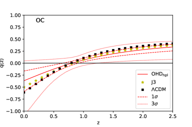
To confirm that the OC model can drive to a late cosmic acceleration, we reconstructed the deceleration parameter using the mean values derived from the different data sets. Figure 9 shows that the $q(z)$ dynamics is similar for the $\Lambda$CDM and OC models when the OHD_hpl, cJLA and J3 constrains are used, i.e., the universe has a late phase of accelerated expansion. Notice that although the confidence levels in the $q(z)$ reconstruction obtained from the SNIa constraints are bigger that those from the OHD_hpl, they are consistent. The difference could be explained by the extra free parameter (nuisance) in the SNIa analysis.

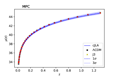
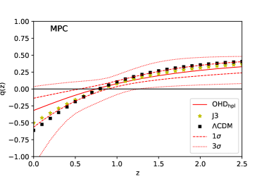
Figure 10 shows the 1D marginalized posterior distributions and the 2D $68\%$, $95\%$, $99\%$ contours for the $\Omega_{m0}$, $h$, $n$ and $l$ parameters of the MPC model obtained from OHD_hpl, cJLA, and J3 with flat (left panel) and Gaussian (right panel) priors on $h$. Considering a flat prior on $h$, the different data sets provide slightly different constraints on $\Omega_{m0}$ and $h$. For instance, the $\mathrm{OHD_{DA}}$ estimates higher (lower) values on $\Omega_{m0}\,(h)$ and SN Ia lower (higher) values. However, the limits are consistent within the $1\sigma$ C. L. For the $n$ and $l$ constraints, we also obtained a marginal tension using different data but they are consistent within the $1\sigma$ C. L. Notice that our constraints include $n=0$ and $l=1$, which reproduces the $\Lambda$CDM dynamics. All our bounds are similar within the $1\sigma$ C.L. to those obtained by other authors, e.g. Li et al. (2012) combining SN Ia, BAO and CMB data measure $n=0.014^{+0.36}_{-0.94}$, $l=1.09^{+1.01}_{-0.46}$, Magaña et al. (2015) using strong lensing features estimate $n=0.41\pm{0.25}$, $l=5.2\pm{2.25}$, Zhai et al. (2017a) provide $n=0.16^{+0.08}_{0.09}$, $l=1.38^{+0.25}_{-0.22}$ from the joint analysis of CMB, BAO plus SN Ia (JLA) data, and Zhai et al. (2017b) give $n=0.02^{+0.26}_{-0.41}$, $l=1.1^{+0.8}_{-0.4}$ from the joint analysis of CMB, BAO, SN Ia, $f\sigma_{8}$ and the $H_{0}$ value from Riess et al. (2016a). In addition, the $\chi_{red}^{2}$ values point out that the $\mathrm{OHD_{DA}}$ provides better (unbiased) MPC constraints and the values from SN Ia data suggest that their errors (cJLA sample) are underestimated. Considering the Gaussian prior on $h$ by Riess et al. (2016b), the OHD, OHD_hpl, and OHD_hw9 probes yield improvements in the MPC constraints (see the $\chi_{red}$ values). For the SN Ia (cJLA) test, there is no significant difference with the flat prior case. Notice that the stringent limits are estimated from the joint analysis (see also Fig. 10). Figure 11 shows the fittings to the OHD_hpl and cJLA data using the OHD_hpl, cJLa and J3 constraints of the MPC parameters and those of the $\Lambda$CDM model with a flat prior on $h$. To propagate the errors on OHD, $\mu(z)$, and $q(z)$, we have used a Monte Carlo approach. For both, OHD and $\mu(z)$ fittings, there is no significant statistical difference between the MPC model and the standard one. In addition, a good agreement at $1\sigma$ is obtained employing the J1, J2 and J4 constraints. In addition, Figure 12 shows the reconstruction of the $q(z)$ parameter using the constraints from the OHD and SN Ia data. For the OHD constraints, the $q(z)$ dynamics for the MPC is in agreement with that of the standard model. When the SN Ia estimations are used, the history of the cosmic acceleration for the MPC model is consistent with the $\Lambda$CDM within the $1\sigma$ and $3\sigma$ C.L. Thus, the MPC scenario is viable to explain the late cosmic acceleration without a dark energy component and its cosmological dynamics is almost indistinguishable from the standard model.

MPC model

(a) Flat prior on $h$

(b) Gaussian prior on $h$

Figure 10: 1D marginalized posterior distributions and the 2D $68\%$, $95\%$, $99.7\%$ confidence levels for the $\Omega_{m0}$, $h$, $n$, and $l$ parameters of the MPC model assuming a flat and Gaussian (h_Riess) prior on $h$.

Figure 11: Fitting to OHD_hpl (top panel) and SN Ia data (bottom panel) using the mean values from the OHD_hpl (red solid lines), cJLA (blue solid lines) and J3 (yellow star and triangle) analysis for $\Lambda$CDM model (black squares) and MPC model when a flat prior on $h$ is considered.

The dashed-lines and dotted-lines represent the $68\%$ and $99.7\%$ confidence levels respectively.

Figure 12: Reconstruction of the deceleration parameter $q(z)$ for the MPC model and $\Lambda$CDM using the constraints from OHD_hpl (top panel) and SN Ia data (bottom panel) when a flat prior on $h$ is considered. The $q(z)$ reconstruction from J3 constraints is shown in both panels. The dashed-lines and dotted-lines represent the $68\%$ and $99.7\%$ confidence levels respectively.

5 Conclusions and Outlooks

In this paper we analyze two alternatives to explain the late cosmic acceleration without a dark energy component: the original (OC) and modified polytropic Cardassian (MPC) models which are also excellent laboratories to study deviations from GR. The Cardassian models establish the modification of the canonical Friedmann equation as a consequence of a braneworld dynamics which emerges from novel ideas of the space-time dimensions and is based on a generalized Einstein-Hilbert action.

To constrain the exponents $n$ and the $n-l$ of the OC and MPC models, we used 51 observational Hubble data, 740 SNIa data points of the JLA sample (fJLA) and 31 binned distance modulus of the compressed JLA sample (cJLA). The OHD compilation contains $31$ points measured using the differential age technique in early-type-galaxies and $20$ points from clustering. These last points are biased due to an underlying $\Lambda$CDM cosmology to estimate the sound horizon at the drag epoch, which is used to compute $H(z)$. Moreover, these data points are estimated taking into account very conservative systematic errors. Therefore, we constructed two homogenized and model-independent samples for the clustering points using a common $r_{d}$ obtained from Planck and WMAP measurements.

We found that the different OHD samples provide consistent constraints on the OC and MPC parameters. In addition, there is no significant differences on the constraints obtained from the cJLA and those estimated from fJLA. Furthermore, we obtained consistent constraints at $3\sigma$ confidence level when different Gaussian priors on $h$ are employed. We performed a joint analysis with the combination of cJLA and one homogenized OHD sample. Our results shown that the OC and MPC free parameters are consistent with the traditional dynamics dictated by the Friedmann equation (see Tables 3-6) containing a cosmological constant (CC). However, in the Cardassian models the extra terms in the canonical Friedmann equation mimic the CC but it comes from the n-term of the energy momentum tensor, unlike in the traditional form where the CC is added by hand in the Friedmann equation. Of course, those problems affecting the CC will be transferred to the interpretation of n-dimensional geometry and, as a consequence, to the emerging of the n-term of the energy-momentum tensor. Therefore, the idea is to interpret and to know the global topology of our Universe to generate a solution for the DE problem and the current Universe acceleration.

Appendix A Compressed JLA sample

$z_{b}$	$\mu_{b}$
0.010	32.953886976
0.012	33.8790034661
0.014	33.8421407403
0.016	34.1185670426
0.019	34.5934459829
0.023	34.9390265264
0.026	35.2520963261
0.031	35.7485016537
0.037	36.0697876073
0.043	36.4345704737
0.051	36.6511105942
0.060	37.1580141133
0.070	37.4301732516
0.082	37.9566163488
0.097	38.2532540406
0.114	38.6128693372
0.134	39.0678507056
0.158	39.3414019038
0.186	39.7921436157
0.218	40.1565346033
0.257	40.5649560582
0.302	40.9052877824
0.355	41.4214174356
0.418	41.7909234574
0.491	42.2314610669
0.578	42.6170470706
0.679	43.0527314851
0.799	43.5041508283
0.940	43.9725734093
1.105	44.5140875789
1.300	44.8218674621

Table 7: Compressed JLA sample which contains 31 binned distance modulus fitted to the full JLA sample by Betoule et al. (2014). The first column is the binned redshift and the second column is the binned distance modulus.

References

- Ade et al. (2014) Ade P. A. R., et al., 2014, Astron. Astrophys., 571, A16
- Ade et al. (2016) Ade P. A. R., et al., 2016, Astron. Astrophys., 594, A13
- Alam et al. (2016) Alam S., et al., 2016, Submitted to: Mon. Not. Roy. Astron. Soc.
- Anderson et al. (2014) Anderson L., et al., 2014, Mon. Not. Roy. Astron. Soc., 439, 83
- Bautista et al. (2017) Bautista J. E., et al., 2017
- Bennett et al. (2013) Bennett C. L., et al., 2013, Astrophys. J. Suppl., 208, 20
- Bernal et al. (2016) Bernal J. L., Verde L., Riess A. G., 2016, J. Cosmology Astropart. Phys., 10, 019
- Betoule et al. (2014) Betoule M., et al., 2014, Astron. Astrophys., 568, A22
- Blake et al. (2012) Blake C., et al., 2012, Mon. Not. Roy. Astron. Soc., 425, 405
- Buchdahl (1970) Buchdahl H. A., 1970, MNRAS, 150, 1
- Carroll (2001) Carroll S. M., 2001, Living Reviews in Relativity, 4, 1
- Cembranos (2009) Cembranos J. A. R., 2009, Phys. Rev. Lett., 102, 141301
- Chuang & Wang (2013) Chuang C.-H., Wang Y., 2013, Mon. Not. Roy. Astron. Soc., 435, 255
- Copeland et al. (2006) Copeland E. J., Sami M., Tsujikawa S., 2006, International Journal of Modern Physics D, 15, 1753
- Deffayet et al. (2002) Deffayet C., Dvali G., Gabadadze G., 2002, Phys. Rev. D, 65, 044023
- Delubac et al. (2015) Delubac T., et al., 2015, Astron. Astrophys., 574, A59
- Farooq et al. (2017) Farooq O., Madiyar F. R., Crandall S., Ratra B., 2017, Astrophys. J., 835, 26
- Feng & Li (2010) Feng C.-J., Li X.-Z., 2010, Phys. Lett., B692, 152
- Font-Ribera et al. (2014) Font-Ribera A., et al., 2014, JCAP, 1405, 027
- Foreman-Mackey et al. (2013) Foreman-Mackey D., Hogg D. W., Lang D., Goodman J., 2013, Publications of the Astronomical Society of the Pacific, 125, 306
- Freese & Lewis (2002) Freese K., Lewis M., 2002, Physics Letters B, 540, 1
- Ganeshalingam et al. (2013) Ganeshalingam M., Li W., Filippenko A. V., 2013, Mon. Not. Roy. Astron. Soc., 433, 2240
- Gaztanaga et al. (2009) Gaztanaga E., Cabre A., Hui L., 2009, Mon. Not. Roy. Astron. Soc., 399, 1663
- Gondolo & Freese (2002) Gondolo P., Freese K., 2002, ArXiv High Energy Physics - Phenomenology e-prints,
- Gondolo & Freese (2003) Gondolo P., Freese K., 2003, Phys. Rev. D, 68, 063509
- Hinshaw et al. (2013) Hinshaw G., et al., 2013, ApJS, 208, 19
- Jimenez & Loeb (2002) Jimenez R., Loeb A., 2002, Astrophys. J., 573, 37
- Komatsu et al. (2011) Komatsu E., et al., 2011, Astrophys. J. Suppl., 192, 18
- Leaf & Melia (2017) Leaf K., Melia F., 2017, preprint, (arXiv:1706.02116)
- Li et al. (2012) Li Z., Wu P., Yu H., 2012, ApJ, 744, 176
- Liang et al. (2011) Liang N., Wu P.-X., Zhu Z.-H., 2011, Research in Astronomy and Astrophysics, 11, 1019
- Maartens (2000) Maartens R., 2000, Phys. Rev. D, 62, 084023
- Maartens (2004) Maartens R., 2004, Living Rev. Rel., 7, 7
- Magaña et al. (2015) Magaña J., Motta V., Cárdenas V. H., Verdugo T., Jullo E., 2015, ApJ, 813, 69
- Mangano et al. (2002) Mangano G., Miele G., Pastor S., Peloso M., 2002, Physics Letters B, 534, 8
- Melia & López-Corredoira (2017) Melia F., López-Corredoira M., 2017, International Journal of Modern Physics D, 26, 1750055
- Moresco (2015) Moresco M., 2015, Mon. Not. Roy. Astron. Soc., 450, L16
- Moresco et al. (2012) Moresco M., et al., 2012, JCAP, 1208, 006
- Moresco et al. (2016) Moresco M., et al., 2016, JCAP, 1605, 014
- Neveu et al. (2017) Neveu J., Ruhlmann-Kleider V., Astier P., Besançon M., Guy J., Möller A., Babichev E., 2017, A&A, 600, A40
- Oka et al. (2014) Oka A., Saito S., Nishimichi T., Taruya A., Yamamoto K., 2014, Mon. Not. Roy. Astron. Soc., 439, 2515
- Randall & Sundrum (1999a) Randall L., Sundrum R., 1999a, Physical Review Letters, 83, 3370
- Randall & Sundrum (1999b) Randall L., Sundrum R., 1999b, Physical Review Letters, 83, 4690
- Ratsimbazafy et al. (2017) Ratsimbazafy A. L., Loubser S. I., Crawford S. M., Cress C. M., Bassett B. A., Nichol R. C., Väisänen P., 2017, Mon. Not. Roy. Astron. Soc., 467, 3239
- Riess et al. (2016a) Riess A. G., et al., 2016a
- Riess et al. (2016b) Riess A. G., et al., 2016b, Astrophys. J., 826, 56
- Sen & Sen (2003a) Sen A., Sen S., 2003a, Phys. Rev. D, 68, 023513
- Sen & Sen (2003b) Sen S., Sen A. A., 2003b, ApJ, 588, 1
- Shi et al. (2012) Shi K., Huang Y. F., Lu T., 2012, MNRAS, 426, 2452
- Shiromizu et al. (2000) Shiromizu T., Maeda K., Sasaki M., 2000, Phys. Rev. D, 62, 024012
- Starobinsky (1980) Starobinsky A., 1980, Physics Letters B, 91, 99
- Stern et al. (2010) Stern D., Jimenez R., Verde L., Kamionkowski M., Stanford S. A., 2010, JCAP, 1002, 008
- Suzuki et al. (2012) Suzuki N., et al., 2012, ApJ, 746, 85
- Wang et al. (2003) Wang Y., Freese K., Gondolo P., Lewis M., 2003, ApJ, 594, 25
- Wang et al. (2017) Wang Y., et al., 2017, MNRAS, 469, 3762
- Wei et al. (2015) Wei J.-J., Ma Q.-B., Wu X.-F., 2015, Adv. Astron., 2015, 576093
- Weinberg (1989) Weinberg S., 1989, Reviews of Modern Physics, 61
- Xu (2012) Xu L., 2012, Eur. Phys. J., C72, 2134
- Yu & Wang (2016) Yu H., Wang F. Y., 2016, Astrophys. J., 828, 85
- Zeldovich (1968) Zeldovich Y. B., 1968, Soviet Physics Uspekhi, 11
- Zhai et al. (2017a) Zhai X.-h., Lin R.-h., Feng C.-j., Li X.-z., 2017a, preprint, (arXiv:1705.09490)
- Zhai et al. (2017b) Zhai Z., Blanton M., Slosar A., Tinker J., 2017b, preprint, (arXiv:1705.10031)
- Zhang & Xia (2016) Zhang M.-J., Xia J.-Q., 2016, JCAP, 1612, 005
- Zhang et al. (2014) Zhang C., Zhang H., Yuan S., Zhang T.-J., Sun Y.-C., 2014, Res. Astron. Astrophys., 14, 1221