Triggering Collapse of the Presolar Dense Cloud Core and Injecting Short-Lived Radioisotopes with a Shock Wave. V. Nonisothermal Collapse Regime

Abstract

Recent meteoritical analyses support an initial abundance of the short-lived radioisotope ⁶⁰Fe that may be high enough to require nucleosynthesis in a core collapse supernova, followed by rapid incorporation into primitive meteoritical components, rather than a scenario where such isotopes were inherited from a well-mixed region of a giant molecular cloud polluted by a variety of supernovae remnants and massive star winds. This paper continues to explore the former scenario, by calculating three dimensional, adaptive mesh refinement, hydrodynamical code (FLASH 2.5) models of the self-gravitational, dynamical collapse of a molecular cloud core that has been struck by a thin shock front with a speed of 40 km/sec, leading to the injection of shock front matter into the collapsing cloud through the formation of Rayleigh-Taylor fingers at the shock-cloud intersection. These models extend the previous work into the nonisothermal collapse regime using a polytropic approximation to represent compressional heating in the optically thick protostar. The models show that the injection efficiencies of shock front material are enhanced compared to previous models, which were not carried into the nonisothermal regime and so did not reach such high densities. The new models, combined with the recent estimates of initial ⁶⁰Fe abundances, imply that the supernova triggering and injection scenario remains as a plausible explanation for the origin of the short-lived radioisotopes involved in the formation of our solar system.

1 Introduction

The discovery of reproducible evidence for live ²⁶Al (Lee et al. 1976), with a half-life of 0.72 Myr, in Ca, Al-rich refractory inclusions (CAIs) from the Allende meteorite led directly to the hypothesis of the injection of core-collapse supernova-derived (CCSN) short-lived radioisotopes (SLRIs) such ²⁶Al (as well as ⁶⁰Fe) into the presolar cloud and the triggering of the collapse of the cloud to form the solar nebula (Cameron & Truran 1977). However, ²⁶Al is also produced in abundance during the Wolf-Rayet (WR) star phase, prior to the supernova explosion of massive stars (e.g., Young 2016), whereas ⁶⁰Fe, with a half-life of 2.6 Myr, is only produced in significant amounts by CCSN and AGB stars. As a result, a high initial level of ⁶⁰Fe is often considered the smoking gun for the supernova triggering and injection hypothesis.

Early estimates of the initial amount of ⁶⁰Fe in chondrules from ordinary chondritic (OC) meteorites implied a ratio of ⁶⁰Fe/⁵⁶Fe $\sim 5-10\times 10^{-7}$ (Tachibana et al. 2006), high enough to require a CCSN for its nucleosynthesis shortly before its incorporation into the earliest solids in the solar nebula. However, subsequent analyses of bulk samples of different meteorite types produced a much lower initial ratio of ⁶⁰Fe/⁵⁶Fe $\sim 1.15\times 10^{-8}$ (Tang & Dauphas 2012), seemingly refuting the smoking gun theory. Using that lower ratio, Young (2014, 2016) argued that there was no need for a recent SN injection, and that the initial abundances of a dozen SLRIs could be explained by the contributions of massive star winds to the general interstellar medium in regions of star formation. However, other studies continued to find high initial ⁶⁰Fe/⁵⁶Fe ratios, now in unequilibrated OC (UOC), of $\sim 7\times 10^{-7}$, $\sim 2-8\times 10^{-7}$, and $\sim 8-11\times 10^{-7}$, respectively (Mishra & Goswami 2014; Mishra & Chaussidon 2014; Mishra et al. 2016). As a result, a mystery arose regarding ⁶⁰Fe analyses of individual chondrules compared to bulk samples.

The puzzling situation with regard to ⁶⁰Fe seems to have been resolved by the work of Telus et al. (2016). Telus et al. (2016) found that the bulk sample estimates were skewed toward low initial ⁶⁰Fe/⁵⁶Fe ratios because of fluid transport of Fe and Ni along chondrule fractures during aqueous alteration on the parent body or during terrestrial weathering. While the initial ⁶⁰Fe/⁵⁶Fe value is still somewhat uncertain, Telus et al. (2017) have found that UOCs appear to have levels of ⁶⁰Ni consistent with initial ratios of ⁶⁰Fe/⁵⁶Fe as high as $5.6\times 10^{-7}$. This value supports a CCSN supernova as a plausible source for many of the SLRIs, and refutes the scenario advanced by Young (2014, 2016), at least regarding ⁶⁰Fe. Furthermore, CCSN nucleosynthesis models by Banerjee et al. (2016) have shown that neutrino spallation reactions can produce the requisite amount of live ¹⁰Be (half-life of 1.4 Myr) found in certain CAIs in a supernova that occurred about 1 Myr prior to CAI formation. Given these recent cosmochemical results, the supernova trigger hypothesis continues to be worthy of detailed investigation.

One variation on the shock-triggered collapse scenario is the injection of CCSN-derived material directly into an already-formed solar nebula (e.g., Oullette et al. 2007, 2010). Parker & Dale (2016) concluded that such a scenario is probably more likely to occur than the original scenario of injection into a pre-collapse cloud core, while Nicolson & Parker (2017) found that disk enrichment was as likely to occur in low mass star clusters as in more massive clusters. Given that we only know about the presence of possibly high initial levels of certain SLRIs in meteorites from our own solar system [cf., Jura et al. (2013) for a different point of view, based on observations of metal-rich white dwarf stars], it is unclear how one can use probabilistic arguments to constrain the formation of a single planetary system in a galaxy that contains billions of planetary systems (cf. Lichtenberg et al. 2016). The crucial question is whether the scenario is possible, rather than if it is probable, given our sample of one. Oullette et al. (2007, 2010) studied SN shock wave injection into the solar nebula, and found that only solid particles larger than $\sim$ 1 $\mu$m can be injected; smaller particles and gas in the SN shock front are unable to penetrate into the much higher density protoplanetary disk. Goodson et al. (2016) performed a similar study of particle injection, but into a molecular cloud rather than a disk, and also found that particles larger than $\sim$ 1 $\mu$m were preferentially injected deep with the target cloud. However, analysis of Al and Fe dust grains in SN ejecta constrain their sizes to be less than 0.01 $\mu$m (Bocchio et al. 2016), effectively severely limiting the value of both of these injection mechanism scenarios.

Vasileiadis et al. (2013) and Kuffmeier et al. (2016) have modeled the evolution of a $\sim 10^{5}M_{\odot}$ Giant Molecular Cloud (GMC), and shown how the SLRI’s ejected by CCSN in the GMC can pollute the surrounding gas to highly variable levels, ranging from ²⁶Al/²⁷Al $\sim 10^{-7}$ to $\sim 10^{-1}$, much higher than the canonical solar system ratio of ²⁶Al/²⁷Al $\sim 5\times 10^{-5}$ (Lee et al. 1976). Ratios of ⁶⁰Fe/⁵⁶Fe were as high $\sim 10^{-3}$ (Kuffmeier et al. 2016), again much higher than any meteoritical estimates. Given that the GMC simulation covered a 3D region 40 pc in extent, with computational cell densities no higher than $\sim 10^{-16}$g cm^-3, data sampled every 0.05 Myr, and minimum grid spacings of 126 AU, this ambitious simulation was unable to follow in detail the interactions of specific supernova shock fronts with any dense molecular cloud cores. Such interactions are the focus of the present series of studies, where SN shocks with $\sim$ 60 AU thicknesses strike clouds and within 0.1 Myr trigger collapse to densities of over $\sim 10^{-11}$ g cm^-3. In fact, star formation in the Vasileiadis et al. (2013) and Kuffmeier et al. (2016) GMC calculation is not the result of SN shock wave triggering, but rather the eventual self-gravitational collapse of pre-stellar cores formed by GMC turbulence over 4 Myr of GMC evolution.

Balazs et al. (2004) presented observational evidence that a supernova shock front triggered the formation of T Tauri stars in the L1251 cloud. As reviewed by Boss (2016), the numerical study of the shock-triggered collapse and injection scenario for the origin of the solar system SLRIs began with the relatively crude three dimensional (3D) models of Boss (1995). Subsequent theoretical models retreated to the higher spatial resolution afforded by axisymmetric, two dimensional (2D) models (e.g., Foster & Boss 1996; Vanhala & Boss 2000), which revealed the role of Rayleigh-Taylor (RT) fingers in the injection mechanism. Boss et al. (2008, 2010) introduced the use of the FLASH adaptive mesh refinement (AMR) code in order to better resolve the thin shock fronts and RT fingers with a reasonable number of spatial grid points, and FLASH has been the basis of our modeling ever since. Boss & Keiser (2013) used 2D FLASH AMR models to study rotating presolar clouds that collapsed to form disks. Boss & Keiser (2014, 2015) extended those models to 3D, with rotational axes either parallel to, or perpendicular to, the direction of propagation of the SN shock front, respectively. Li et al. (2014) and Falle et al. (2017) used AMR codes to study the triggering of collapse by isothermal shocks striking non-rotating, isothermal, Bonnor-Ebert spheres.

All of the previous FLASH AMR code models have been restricted to optically thin regimes ($<10^{-13}$ g cm^-3) where molecular line cooling by H₂O, CO, and H₂ are effective at cooling the shock-compressed regions (Boss et al. 2008, 2010; Boss & Keiser 2013, 2014, 2015). The Vasileiadis et al. (2013) and Kuffmeier et al. (2016, 2017) GMC calculations have a similar limitation to optically thin regimes. In our case, this restriction allows one to learn if a given target cloud can be shocked into collapse, but it prohibits following the calculation to much later times, after the central protostar forms, surrounded by infalling, rotating gas and dust that will form the solar nebula. To a first approximation, nonisothermal effects in optically thick regimes can be approximated by the use of a simple polytropic ($\gamma=7/5$) pressure law, mimicking the compressional heating in molecular hydrogen encountered at densities above $\sim 10^{-13}$ g cm^-3 (e.g., Boss 1980). Adding this new handling of the equation of state in the nonisothermal regime is the motivation for the 3D models presented in this paper.

2 Numerical Hydrodynamics Code

As with the previous papers in this series, the models were calculated with the FLASH2.5 AMR hydrodynamics code (Fryxell et al. 2000). Full details about the implementation of FLASH 2.5 may be found in Boss et al. (2010). We restrict ourselves here to noting what has been changed in the present models compared to the most recent previous 3D models (i.e., Boss & Keiser 2014, 2015). As before, a color field is used to follow the transport of the gas and dust initially residing in the shock front.

Initially, the low density target cloud and the surrounding gas are isothermal at 10 K, whereas the SN shock front and post-shock gas are isothermal at 1000 K. The FLASH code follows the subsequent compressional heating as well as cooling of the interaction between the shock and the cloud by the molecular species H₂O, CO, and H₂, resulting in a radiative cooling rate appropriate for rotational and vibrational transitions of optically thin, warm molecular gas (Boss et al. 2010). As a result, the shock front temperatures are unchanged from those in the previous simulations. The primary change is then the use of a polytropic equation of state when densities high enough to produce an optically thick cloud core arise, i.e., for densities above some critical density $\rho_{cr}\sim 10^{-13}$ g cm^-3 (Boss 1980). Molecular gas cooling is then prohibited for densities greater than $\rho_{cr}$, when the gas pressure $p$ depends on the gas density $\rho$ as $p\propto\rho^{\gamma}$, where the polytropic exponent $\gamma$ equals 7/5 for molecular hydrogen gas. We tested several different variations in $\rho_{cr}$ in order to find the value that was best able to reproduce the dependence of the central temperature on the central density found in the spherically symmetrical collapse models of Vaytet et al. (2013), who performed detailed multigroup radiative hydrodynamics calculations of the collapse of solar-mass uniform density spheres.

3 Initial Conditions

Table 1 lists the variations in the initial conditions for the models, which are all variations on two rotating models considered previously in this series (e.g., Boss & Keiser 2014): a 2.2 $M_{\odot}$ cloud with a radius of 0.053 pc and a Bonnor-Ebert radial density profile, with solid body rotation about the $\hat{y}$ axis (the direction of propagation of the shock wave) at an angular frequency of $\Omega_{i}=10^{-14}$ or $10^{-13}$ rad s^-1. The shock wave propagates toward the $-\hat{y}$ direction with a shock speed of 40 km s^-1 with an initial shock width of $3\times 10^{-4}$ pc and an initial shock density of $7.2\times 10^{-18}$ g cm^-3. In order to test the sensitivity of the results to the presence of noisy initial conditions, two models were run with random noise in the interval of [0,1] inserted in the ambient gas surrounding the uniform density target cloud, resulting in the ambient medium having density variations ranging from a maximum density of $1.2\times 10^{-20}$ g cm^-3 to a minimum density 40 times lower, $3\times 10^{-22}$ g cm^-3.

Boss et al. (2010) studied the effect of shock wave speeds ranging from 1 km s^-1 to 100 km s^-1, finding that sustained triggered collapse was only possible for shock speeds in the range of 5 km s^-1 to 70 km s^-1: slower shocks failed to inject shock wave material, while faster shocks shredded the clouds and did not trigger collapse. Boss & Keiser (2010) presented results for shock speeds of 40 km s^-1 and varied shock thicknesses, as high as 100 times thicker than used here, in order to distinguish between relatively thin SN shocks and relatively thick planetary nebula winds from AGB stars. They found that 40 km/s shocks thicker than those considered here shredded the target clouds without inducing sustained collapse, even when the shock densities were lower than assumed here, and so concluded that an AGB star was an unlikely source of the solar system SLRIs. Boss et al. (2010) noted out that these simulations are meant to represent the radiative phase of SN shock wave evolution, which occurs after the Sedov blast wave phase (Chevalier 1974). In the radiative phase, the shock sweeps up gas and dust while radiatively cooling, as is modeled here.

The FLASH 2.5 code AMR numerical grids start with 6 grid blocks along the $\hat{x}$ and $\hat{z}$ directions, and either 9 or 12 grid blocks in the $\hat{y}$ direction (the latter for the six models with $y_{min}=-2.0\times 10^{17}$ cm), with each grid block consisting of $8^{3}$ cells. Models started with either 3 or 4 levels of refinement (with each level refined by a factor of two) on the initial grid blocks. The number of levels of grid refinement was increased during the evolutions to as many as 8 levels when permitted by the memory limitations of the flash cluster nodes used for the computations. The initial grid blocks thus have 48 cells in $x$ and $z$, and 72 or 96 in $y$. With 4 levels of refinement, i.e., 3 levels beyond the initial grid blocks, there are $2^{3}\times 48=384$ cells initially in $x$ and $z$, yielding an initial cell size of $10^{15}$ cm $\approx 3\times 10^{-4}$ pc in all three coordinate directions (the cells are cubical). With the maximum of 8 levels of refinement used, the minimum cell size drops by a factor of 16 to $\approx 6\times 10^{13}$ cm $\approx 2\times 10^{-5}$ pc.

4 Results

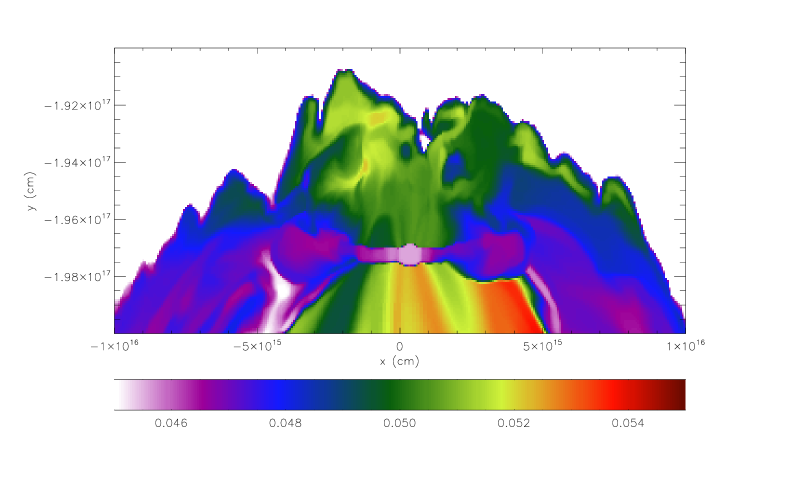
Figure 7: Model J color field (shock front matter) cross-section ($z$ = 0) at 0.0868 Myr.

Models A through I varied primarily in the assumed value of $\rho_{cr}$, in order to assess the best choice for approximating the results obtained for a full radiative transfer solution for a collapsing dense cloud core. Vaytet et al. (2013) found that the evolution of the central temperature of a collapsing solar-mass cloud did not differ greatly between multigrid radiative transfer simulations with 20 different radiation frequency bands and grey simulations with a single effective frequency band (cf. their Figure 7), that is, at a given central density, the central temperatures in the two simulations agreed to within about 10%. They found that central temperatures $T_{c}$ began to rise above the initial cloud temperature of 10 K for central densities above $\rho_{c}\sim 10^{-13}$ g cm^-3, as expected (e.g., Boss 1980), with $T_{c}\approx 26$ K at $\rho_{c}=10^{-12}$ g cm^-3. In fact, the dependence of $T_{c}$ on $\rho_{c}$ in Figure 7 of Vaytet et al. (2013) is almost exactly $T_{c}\propto\rho_{c}^{2/5}$, as expected for a polytropic gas composed primarily of molecular hydrogen with $\gamma=7/5$.

Model A was calculated with $\rho_{cr}=10^{-14}$ g cm^-3, resulting in a rotationally flattened disk orbiting around a dense central protostar, but with a central temperature $T_{c}\approx 300$ K when $\rho_{c}\sim 10^{-13}$ g cm^-3, much too hot compared to the Vaytet et al. (2013) results. Similarly, models B and C, both with $\rho_{cr}=10^{-13}$ g cm^-3 but with different initial rotation rates, produced disks with $T_{c}\approx 200$ K and $\approx 100$ K, respectively, when $\rho_{c}\sim 10^{-13}$ g cm^-3, again too hot. Models D and E, both with $\rho_{cr}=3\times 10^{-13}$ g cm^-3, were also too hot, with $T_{c}\approx 150$ K at $\rho_{c}\sim 10^{-13}$ g cm^-3. On the other hand, models H and I, both with $\rho_{cr}=10^{-12}$ g cm^-3, were much too cool, with $T_{c}\approx 10$ K when $\rho_{c}\sim 10^{-12}$ g cm^-3, considerably lower than the Vaytet et al. (2013) value of $\approx$ 26 K at that density. As a result, yet another two models were calculated, models F and G, with $\rho_{cr}=5\times 10^{-13}$ g cm^-3, and these models finally yielded a reasonable central temperature of $\approx$ 20 K when $\rho_{c}\sim 3\times 10^{-13}$ g cm^-3. As a result, $\rho_{cr}=5\times 10^{-13}$ g cm^-3 was adopted as the best approximation for reproducing the Vaytet et al. (2013) results.

While these models were able to calibrate the choice of $\rho_{cr}$, it became clear that a second set of models would need to be calculated with a longer box in the $y$ direction. This is because the use of the new handling of the thermodynamics in the optically thick central protostar meant that the calculations could be carried forward farther in time than in the past, beyond when the collapsing protostars and disks, accelerated by the shock to speeds of several km/sec, reached the ends of the computational volume in models A through I. As a result, models J through O were calculated with the total computational volume expanded by about a third along the direction of the shock wave propagation. In order to preserve the same grid resolution, this meant that the number of computational blocks in the $\hat{y}$ direction had to be increased from 9 to 12 (Table 1). Each of these models required about two months of time to run while using 88 cores on the DTM flash cluster, for a total of about 130K core-hours.

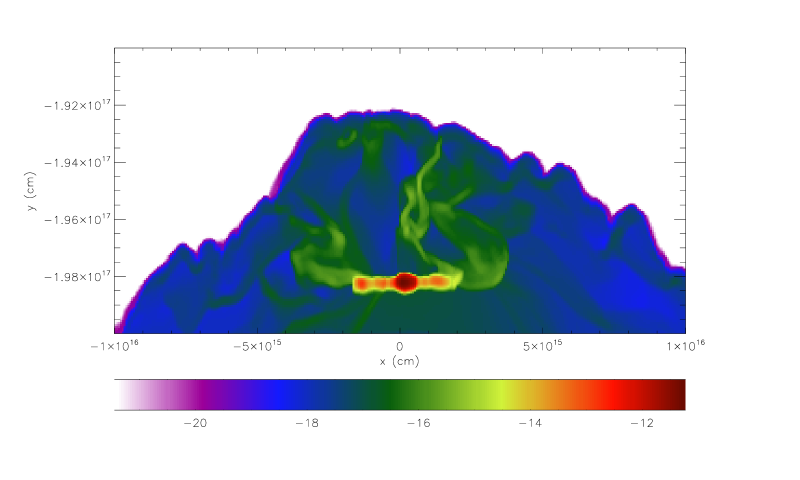
Figure 1: Model L log density cross-section ($z$ = 0) at 0.0869 Myr.

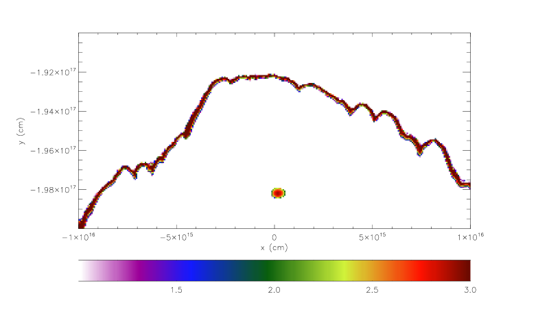
Figure 2: Model L log temperature cross-section ($z$ = 0) at 0.0869 Myr. The corrugated structure is a reflection of the Rayleigh-Taylor fingers responsible for shock wave matter injection.

Model L is indicative of the results for all six models with the extended computational grid. Figure 1 shows that the model L cloud has collapsed and formed a well-resolved central protostar orbited by a rotating, flattened protostellar disk, aligned perpendicular to the rotation axis ($\hat{y}$) of the initial target cloud (see Boss & Keiser 2015 for the results of models when the initial rotation axis of the cloud is perpendicular to the direction of motion of the shock front). The disk in Figure 1 is very similar in size to the corresponding disk seen in Figure 2 of Boss & Keiser 2015. The disk mass is about 0.3 $M_{\odot}$, while the central protostar has a mass of about 0.5 $M_{\odot}$, implying that this is still a protostellar disk. The maximum density in the protostar has risen to $\sim 10^{-11}$ g cm^-3, well within the nonisothermal regime, and continues to rise slowly. Figure 2 shows the temperature distribution for model L at the same time as Figure 1. The highest temperatures (up to 1000 K) occur in the shock front, while the maximum temperature at the center of the protostar is $\sim$ 750 K. This central temperature is considerably higher than that expected at this central density, based on the spherically symmetric collapse models of Vaytet et al. (2013), where the relevant central temperature was only about 56 K. Evidently the FLASH 2.5 implementation of the simple polytropic approximation fails to be valid at such high densities. Even though the model could be computed farther in time than shown in Figures 1 and 2 by extending the computational grid even further in the $-\hat{y}$ direction, the limited validity of the polytropic approximation argues against such a continuation. Clearly then these models provide a bounding model compared to our previous models, where the central protostellar temperature remained fixed at 10 K as the nonisothermal regime was approached and entered: these models show what happens when the protostar eventually becomes hotter than it should in a proper calculation with radiative transfer. In either case, the shock wave is able to trigger the formation and sustained self-gravitational collapse of a central protostar, accompanied by the formation of a rotating protostellar disk. The models with higher initial rotation rates (models K and M) formed disks roughly twice as wide as in model L, and the models with random noise in the initial density distribution (models N and O) evolved very much like the corresponding models without any initial noise.

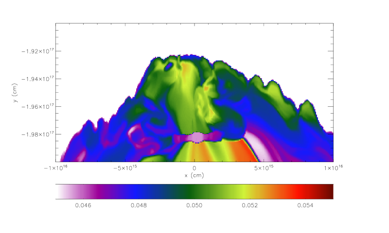
Figure 3: Model L color field (shock front matter) cross-section ($z$ = 0) at 0.0869 Myr.

The second requirement for the success of the supernova triggering and injection scenario is to examine the injection of material originally residing in the shock front into the collapsing protostar and disk. Figure 3 shows that this requirement has been met as well in these nonisothermal regime models. Figure 3 shows that the color field, which is derived from the shock front, where it originally had unit space density, is distributed throughout the protostar, disk, and surrounding envelope. The color field space density is on the order of 0.05 units, meaning it has been diluted by about a factor of 20 compared to its original space density in the shock front. Interestingly, the color field is significantly smaller inside the central protostar than in the surrounding envelope, implying that the outer protoplanetary disk should be endowed with a higher space density of SLRIs than the central protostar and the innermost disk, as suggested by early 2D models by Foster & Boss (1996, 1997).

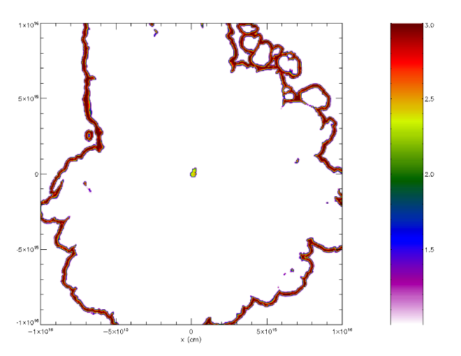
Figure 5: Model L log temperature cross-section in midplane ($y=-1.98\times 10^{17}$ cm) of disk at 0.0869 Myr. The corrugated structure is a reflection of the Rayleigh-Taylor fingers responsible for shock wave matter injection.

Figures 4, 5, and 6 display the cloud density, temperature, and color fields for model L at the same time as in Figures 1, 2, and 3, plotted now in the midplane of the edge-on disk evident in the first three figures. The central protostar is seen clearly in Figure 4, along with a large scale, $\sim$ 200 AU radius, swirling disk in the process of forming and reaching quasi-equilibrium. Figure 5 shows that while the central protostar has heated appreciably, the disk is largely isothermal at 10 K, as expected, as this disk is composed of gas well below the assumed nonisothermal regime critical density $\rho_{cr}=5\times 10^{-13}$ g cm^-3 for model L. The contours of the hot shock front gas in Figure 5 give an indication of the remnants of the Rayleigh-Taylor fingers responsible for shock front injection. Figure 6 again shows that the central protostar does not receive as large a dose of SLRIs as the forming disk, or the envelope material that is on the periphery of the disk. Figures 3 and 6 imply that SLRIs doses could vary by as much as 20% between the central and outer regions of this protostar and disk system.

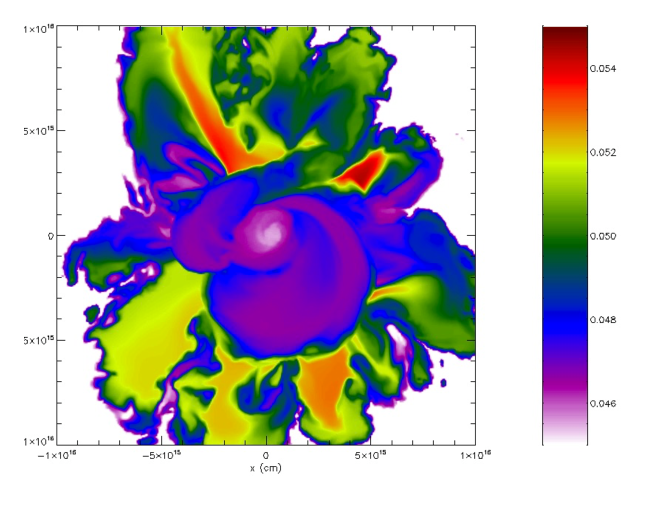
Figure 8: Model J color field (shock front matter) cross-section in midplane ($y=-1.973\times 10^{17}$ cm) of disk at 0.0868 Myr.

In order to test the sensitivity of the above results to the choice of $\rho_{cr}$, we now consider model J, which is identical to model L, except for having $\rho_{cr}=10^{-12}$ g cm^-3 instead of $\rho_{cr}=5\times 10^{-13}$ g cm^-3. Figures 7 and 8 depict the color field distributions in the same two projections as for model L in Figures 3 and 6, respectively. It can be seen by comparison that the color field distributions are quite similar overall, differing only in the fine detail. Evidently the precise choice of $\rho_{cr}$ has little effect on the outcome of the collapse, and in particular on the degree and extent of the injection of shock front SLRIs into the resulting protostar and disk system.

Figures 3 and 7 show that the space density of the color field inside the collapsing protostar and disk is $\approx 0.046$ (dimensionless units) for both models. Model 40-200-0.1-14 of Boss & Keiser (2014) shows that for the same model parameters, but without the nonisothermal heating, the color field in the collapsing region (their Figure 6) is $\approx 0.025$. Given that the present models have been advanced farther in time as a result of the nonisothermal handling of the densest regions, to densities roughly ten times higher, the new models show that the injection efficiency tends to increase with time. As noted by Boss & Keiser (2015), injection efficiencies also tend to increase along with the amount of mass contained in the collapsing region. This is to be expected by noting that the color field surrounding and falling onto the disks seen in Figure 3 and 7 is largely more enriched in SLRIs than the material already injected into the disk, implying that the amount of injected SLRIs should continue to increase as the collapse proceeds, at least to a certain extent. Defining the injection efficiency factor $f_{i}$ as the fraction of the incident shock wave material that is injected into the collapsing cloud core, leads to an estimate of $f_{i}\approx 0.045$ for models L and J, somewhat higher than the value of $f_{i}\approx 0.034$ for the comparable isothermal model from Boss & Keiser (2014). Given that the values of $f_{i}$ found by Boss & Keiser (2014) led to dilution factors at the low end of the range estimated by Takigawa et al. (2008) to be necessary to explain the initial SLRI abundances when derived from a core collapse SNe, the evidence for an increase in $f_{i}$ found in the present models, as well as those of Boss & Keiser (2015), lends further support in favor of the Type II supernova triggering and injection scenario for the solar system.

5 Dilution Factors

The geometric dilution factor $D_{g}$ may be defined as the fraction of the total amount of mass in the SNR that is incident upon a target cloud of radius $r$ lying at a distance $R$ from the stellar remnant and is given by $D_{g}=r^{2}/4R^{2}$. For our target cloud with $r=0.053$ pc, and assuming a nominal distance $R=5$ pc (e.g., the radius of the Cygnus loop SNR, Blair et al. 1999), $D_{g}\approx 3\times 10^{-5}$. $D_{g}$ is the maximum fraction of the total amount of SN-ejected material that can be injected into the target cloud, assuming 100% injection efficiency. For a 25 $M_{\odot}$ pre-supernova star and a neutron star remnant, then, at most $\approx 7.2\times 10^{-4}M_{\odot}$ of SN-derived matter can be injected into the target cloud, based on geometric dilution alone, assuming a nominal distance of 5 pc.

Boss & Keiser (2014) noted that geometric dilution is not the dilution factor used their previous studies and in cosmochemical estimates of initial SLRI abundances (e.g., Takigawa et al. 2008). This latter dilution factor $D$ is defined as the ratio of the amount of mass derived from the supernova to the amount of mass derived from the target cloud. A SNR with an initial speed of $\sim 4000$ km s^-1 must be slowed down considerably by snowplowing the intervening interstellar medium (ISM) in order to reach speeds of $\sim 40$ km s^-1 that do not result in cloud shredding (e.g., Boss et al. 2010). The factor $\beta$ is defined as the ratio of shock front mass originating in the SN to the mass swept-up in the intervening ISM, leading to $\beta\approx 0.01$ for a SNR shock slowed down by a factor of $\sim$ 100 (e.g., Boss & Keiser 2012). For the models considered here, the amount of mass in the shock front that is incident on the target cloud is 0.31 $M_{\odot}$, so that the amount of shock front mass from the SN that is injected into the cloud is 0.31 $f_{i}\beta M_{\odot}$. For a solar-mass protostar, then, $D\approx 0.31f_{i}\beta$. Given that models L and J led to $f_{i}\approx 0.045$, and taking $\beta\approx 0.01$, we get $D\approx 1.4\times 10^{-4}$. This dilution factor is on the lower end of cosmochemical estimates of $D$ in the range of $1.3\times 10^{-4}$ to $1.9\times 10^{-3}$ for pre-supernova stars with masses of 25 $M_{\odot}$ and 20 $M_{\odot}$, respectively (Takigawa et al. 2008).

If $D\approx 1.4\times 10^{-4}$, then for a solar-mass total system mass, the total amount of SN material must be $\approx 1.4\times 10^{-4}$ $M_{\odot}$, which is 5.1 times smaller than the maximum permitted by geometric dilution of $\approx 7.2\times 10^{-4}M_{\odot}$, for the parameters assumed in these estimates. Given that $f_{i}\approx 0.045$, this implies that geometric dilution would limit the amount of SN material to be at most $\approx 3.2\times 10^{-5}M_{\odot}$, i.e., about 4.4 times less is required for $D\approx 1.4\times 10^{-4}$. This implies that in order for this $D$ value to agree with $D_{g}$, the target cloud must have been closer than 5 pc away, e.g., at a distance of $\sim 2.4$ pc, in order to increase $D_{g}$ by a factor of 4.4. A consistent result for the injection efficiency based on estimates of both $D$ and $D_{g}$, at least for a 25 $M_{\odot}$ pre-supernova star, might then require that the target cloud lie about 2.4 pc from the pre-supernova star, or perhaps that the pre-supernova star was more massive than 25 $M_{\odot}$.

The W44 SNR is observed to be compressing an adjacent molecular cloud at a phase when the W44 SNR has a radius of about 11 pc (Reach et al. 2005), considerably more distant than the 2.4 pc suggested above. The Cas A SNR has a radius of only about 1.5 pc (e.g., Krause et al. 2008), but is not close to a GMC region. A consistent result may require a close association between a target molecular cloud core and a massive, pre-supernova star. Oullette et al. (2010), e.g., proposed having a SN inject SLRIs into an already formed protoplanetary disk lying only 0.3 pc away. Such a close association is supported by observations of the Eagle Nebula (M16), where dense cloud cores are being irradiated by a cluster of O stars (some as massive as 80 $M_{\odot}$) only about 1 pc away.

Yet another plausible possible solution to the consistency problem involves the fact that SN ejecta are quite clumpy, with large variations in the abundances of SLRIs such as ⁴⁴Ti (factors of 4 or more) having been observed in the Cas A SNR (Grefenstette et al. 2014), implying that core collapse SN explosions can be highly asymmetric. Hence discrepancies on the order of factors of 4 or more in SLRI abundances could be simply explained as a result of the presolar cloud having been triggered into collapse by a particularly SLRI-rich, dense portion of a SNR. Clearly there are several plausible means for reconciling differing estimates of $D_{g}$ and $D$.

6 Discussion

Sahijpal & Goswami (1998) proposed that the absence of evidence for live ²⁶Al in the rare FUN (Fractionation Unknown Nuclear) CAIs was a result of the formation of the FUN inclusions prior to normal CAIs from collapsing gas and dust interior to the outer collapsing regions containing the freshly injected SN SLRIs, as had been suggested by the early shock triggered collapse models of Foster & Boss (1996, 1997) and as can be seen to a lesser extent in Figures 3 and 7 for the present models. MacPherson & Boss (2011) suggested instead that the FUN inclusions may have originated in a SLRI-poor young stellar object (YSO), ejected by the YSO’s bipolar outflow, and transported to a presolar cloud core in the same star-forming region. Kuffmeier et al. (2016) have argued against both of these suggestions, in the latter case on the basis that the inclusions would have to come from more than $\sim$ 0.25 pc away, which they judged to be unrealistic. With regard to the former suggestion, Kuffmeier et al. (2016) included as a second step zoom-in calculations of the GMC regions where eleven low mass stars formed, represented in the GMC code as sink particles, with a focus on the SLRI levels in the immediate vicinity (50 AU or 1000 AU) of the sink particles. The SLRI ratios were uniformly homogeneous at varied levels, implying there should be no variation in the SLRI ratios during the accretion process. However, Kuffmeier et al. (2016) did find SLRI ratio variations during the late phases, $\sim$ 0.1 Myr after sink particle formation. For one star, the ²⁶Al/²⁷Al ratio of accreted material increased by a factor of 2 after 0.16 Myr, but this heterogeneity was attributed to the fact that the sink particle had already accreted most of the gas in its vicinity, allowing more distant gas to be accreted. In fact, because shock-triggered star formation does not occur in the Kuffmeier et al. (2016) models, there is little mixing between the hot, low density GMC regions with fresh SLRIs, and the cool, high density gas in pre-stellar cores. The models presented here, on the other hand, are specifically intended to explore RT injection of fresh SLRIs carried by SN shocks into pre-stellar cores, a process not studied by the Kuffmeier et al. (2016) simulation. Kuffmeier et al. (2017) presented further zoom-in analysis of the Vasileiadis et al. (2013) and Kuffmeier et al. (2016) GMC simulation, showing evidence for strongly heterogeneous accretion of gas and dust in space and time, though they did not address the question of the possible implications of this heterogeneity for the FUN inclusions.

Larsen et al. (2016) presented analyses of achondritic meteorites, and a few chondrites, which they interpreted as evidence of initial spatial heterogeneity of the ²⁶Al/²⁷Al ratio. Larsen et al. (2016) proposed that ²⁶Al was fractionated by thermal processing of the carrier dust grains into gas and dust, which thereafter separated and retained different ²⁶Al/²⁷Al ratios, resulting in a solar nebula with a heterogeneous ²⁶Al distribution, with initial ²⁶Al/²⁷Al ratios varying from $\sim 1-2\times 10^{-5}$ in the inner nebula to $\geq 2.7\times 10^{-5}$ in the outer nebula, compared to an initial canonical ratio of $5.25\times 10^{-5}$ in CAIs. This interpretation relies on the mechanism suggested by Trinquier et al. (2009) and Schiller et al. (2015), who claimed that newly-synthesized SLRIs would be carried by grains that are more thermally labile than the older grains carrying more ancient nucleosynthetic products, resulting in the nebular gas being enriched in ²⁶Al compared to the dust. Kuffmeier et al. (2016) appealed to this same explanation to account for the lack of evidence for live ²⁶Al in FUN inclusions, and extended this argument to the case of ⁶⁰Fe, which they found to be highly overabundant in their sink particles compared to the solar system’s initial inventory. They argued that the carrier phase of the ⁶⁰Fe must be even more volatile than that for the ²⁶Al, so that both SLRIs could be selectively removed from the dust grains that would go on to form the CAIs. However, given that nearly all SNR dust grains are expected to be sub-micron in size (Bocchio et al. 2016), even if some of these grains were thermally evaporated in the infalling presolar cloud, or in the solar nebula, and others were not, to first order these small grains will be transported and mixed along with the gas (e.g., Bate & Loren-Aguilar 2017), eliminating the chance of any large-scale isotopic fractionation that might survive in the solar nebula. Solid particles need to grow to roughly cm-size before appreciable decoupling of their orbital motions from that of the disk gas occurs (e.g., Boss 2015).

7 Conclusions

These 3D triggering and injection models have investigated the effects of the loss of molecular line cooling once the target cloud becomes optically thick at densities above $\sim 10^{-13}$ g cm^-3, when the collapsing regions begin to heat above 10 K, but continue their collapse toward the formation of the first protostellar core at a central density of $\sim 10^{-10}$ g cm^-3 (e.g., Boss & Yorke 1995). The models show that the SLRI injection efficiencies ($f_{i}$) tend to increase as the amount of collapsing matter increases, and as the central density approaches that of the formation of the first protostellar core. These new values of $f_{i}\approx 0.045$, combined with previously estimated dilution factors for core collapse SNRs (Boss & Keiser 2014), produce an improved agreement with the predicted dilution factors needed to explain the solar system’s SLRIs (Takigawa et al. 2008) in the context of the supernova triggering and injection scenario. Ideally, these models will be able to tie a SNR producing similar injection efficiencies to a specific core-collapse SNe nucleosynthesis model, rather than having to invoke a generic GMC scenario (e.g., Kuffmeier et al. 2016) involving a mixture of SNe contributions and massive star winds (e.g., Young 2014, 2016), over a time period of several Myr, to explain the origin of the solar system SLRIs.

The FLASH 4.3 code allows the use of sink particles to represent the central protostars, sidestepping the issue of resolving the thermal evolution of the growing protostar beyond the first core. Given the evident need to further explore the implications for the triggering and injection scenario, a set of FLASH 4.3 calculations with sink particles is presently underway on the flash cluster, and the results will be presented in a future paper.

Table 1: Initial conditions for the models: initial target cloud rotation rates ($\Omega_{i}$, in rad s^-1), critical density for polytropic pressure law ($\rho_{cr}$, in g cm^-3), number of initial grid blocks in $\hat{y}$ direction ($N_{y}$), minimum $y$ grid value ($y_{min}$, in cm), initial number of levels of refinement ($N_{i}$), final number of levels of refinement ($N_{f}$), and whether the initial ambient density distributions were uniform or had random noise.

Model	$\Omega_{i}$	$\rho_{cr}$	$N_{y}$	$y_{min}$	$N_{i}$	$N_{f}$	density
A	$10^{-14}$	$10^{-14}$	9	0.0	4	6	uniform
B	$10^{-14}$	$10^{-13}$	9	0.0	4	6	uniform
C	$10^{-13}$	$10^{-13}$	9	0.0	4	5	uniform
D	$10^{-14}$	$3\times 10^{-13}$	9	0.0	4	5	uniform
E	$10^{-13}$	$3\times 10^{-13}$	9	0.0	4	5	uniform
F	$10^{-14}$	$5\times 10^{-13}$	9	0.0	4	8	uniform
G	$10^{-13}$	$5\times 10^{-13}$	9	0.0	4	7	uniform
H	$10^{-14}$	$10^{-12}$	9	0.0	4	5	uniform
I	$10^{-13}$	$10^{-12}$	9	0.0	4	5	uniform
J	$10^{-14}$	$10^{-12}$	12	$-2.0\times 10^{17}$	4	8	uniform
K	$10^{-13}$	$10^{-12}$	12	$-2.0\times 10^{17}$	4	7	uniform
L	$10^{-14}$	$5\times 10^{-13}$	12	$-2.0\times 10^{17}$	4	8	uniform
M	$10^{-13}$	$5\times 10^{-13}$	12	$-2.0\times 10^{17}$	4	6	uniform
N	$10^{-14}$	$5\times 10^{-13}$	12	$-2.0\times 10^{17}$	3	7	noise
O	$10^{-13}$	$5\times 10^{-13}$	12	$-2.0\times 10^{17}$	3	8	noise

Figure 4: Model L log density cross-section in midplane ($y=-1.98\times 10^{17}$ cm) of disk at 0.0869 Myr.

Figure 6: Model L color field (shock front matter) cross-section in midplane ($y=-1.98\times 10^{17}$ cm) of disk at 0.0869 Myr.

References

- (1)
- (2) Balazs, L. G., Abraham, P., Kun, M., Kelemen, J., & Toth, L. V. 2004, A&A, 425, 133
- (3)
- (4) Bate, M. R., & Loren-Aguilar, P. 2017, MNRAS, 465, 1089
- (5)
- (6) Banerjee, P., Qian, Y.-Z., Heger, A., & Haxton, W. C. 2016, Nature Communications, 7:13639
- (7)
- (8) Blair, W. P., Sankrit, R., Raymond, J. C., & Long, K. S. 1999, AJ, 118, 942
- (9)
- (10) Bocchio, M., Marassi, S., Schneider, R., Bianchi, S., Limongi, M., & Chieffi, A., 2016, A&A, 587, A157
- (11)
- (12) Boss, A. P. 1980, ApJ, 242, 699
- (13)
- (14) Boss, A. P. 1995, ApJ, 439, 224
- (15)
- (16) Boss, A. P. 2015, ApJ, 807, 10
- (17)
- (18) Boss, A. P. 2016, in Handbook of Supernovae, eds. A. W. Alsabti, P. Murdin (Switzerland: Springer)
- (19)
- (20) Boss, A. P., & Keiser, S. A. 2010, ApJL, 717, L1
- (21)
- (22) Boss, A. P., & Keiser, S. A. 2013, ApJ, 770, 51
- (23)
- (24) Boss, A. P., & Keiser, S. A. 2014, ApJ, 788, 20
- (25)
- (26) Boss, A. P., & Keiser, S. A. 2015, ApJ, 809, 103
- (27)
- (28) Boss, A. P., & Yorke, H. A. 1995, ApJ, 439, L55
- (29)
- (30) Boss, A. P., Ipatov, S. I., Keiser, S. A., Myhill, E. A., & Vanhala, H. A. T. 2008, ApJ, 686, L119
- (31)
- (32) Boss, A. P., Keiser, S. A., Ipatov, S. I., Myhill, E. A., & Vanhala, H. A. T. 2010, ApJ, 708, 1268
- (33)
- (34) Cameron, A. G. W., & Truran, J. W. 1977, Icarus, 30, 447
- (35)
- (36) Chevalier, R. 1974, ApJ, 188, 501
- (37)
- (38) Falle, S. A. E. G., Vaidya, B., & Hartquist, T. W. 2017, MNRAS, 465, 260
- (39)
- (40) Foster, P. N., & Boss, A. P. 1996, ApJ, 468, 784
- (41)
- (42) Foster, P. N., & Boss, A. P. 1997, ApJ, 489, 346
- (43)
- (44) Fryxell, B., Olson, K., Ricker, P., et al. 2000, ApJS, 131, 273
- (45)
- (46) Goodson, M. D., Luebbers, I., Heitsch, F., & Frazer, C. C. 2016, MNRAS, 462, 2777
- (47)
- (48) Grefenstette, B. W., et al. 2014, Nature, 506, 339
- (49)
- (50) Jura, M., Xu, S., & Young, E. D. 2013, ApJL, 775, L41
- (51)
- (52) Krause, O., et al. 2008, Science, 320, 1195
- (53)
- (54) Kuffmeier, M., Mogensen, T. F., Haugbolle, T., Bizzarro, M., & Nordlund, A. 2016, ApJ, 826, 22
- (55)
- (56) Kuffmeier, M., Haugbolle, T., & Nordlund, A. 2017, ApJ, in revision
- (57)
- (58) Larsen, K. K., Schiller, M., & Bizzarro, M. 2016, Geochim. Cosmochim. Acta, 176, 295
- (59)
- (60) Lee T., Papanastassiou, D. A., & Wasserburg, G. J. 1976, Geophys. Res. Lett., 3, 109
- (61)
- (62) Li, S., Frank, A., & Blackman, E. G. 2014, MNRAS, 444, 2884
- (63)
- (64) Lichtenberg, T., Parker, R. J., & Meyer, M. R. 2016, MNRAS, 462, 3979
- (65)
- (66) MacPherson, G. J., & Boss, A. P. 2011, PNAS,108, 19152
- (67)
- (68) Mishra, R. K., & Chaussidon, M. 2014, EPSL, 398, 90
- (69)
- (70) Mishra, R. K., & Goswami, J. N. 2014, Geochim. Cosmochim. Acta, 132, 440
- (71)
- (72) Mishra, R. K., Marhas, K. K., & Sameer 2016, EPSL, 436, 71
- (73)
- (74) Nicholson, R. B., & Parker, R. J. 2017, MNRAS, 464, 4318
- (75)
- (76) Ouellette, N., Desch, S. J., & Hester, J. J. 2007, ApJ, 662, 1268
- (77)
- (78) Ouellette, N., Desch, S. J., & Hester, J. J. 2010, ApJ, 711, 597
- (79)
- (80) Parker, R. J., & Dale, J. E. 2016, MNRAS, 456, 1066
- (81)
- (82) Reach, W. T., Rho, J., & Jarrett, T. H. 2005, ApJ, 618, 297
- (83)
- (84) Sahijpal, S., & Goswami, J. N. 1998, ApJL, 509, L137
- (85)
- (86) Schiller, M., Paton, C., & Bizzarro, M. 2015, Geochim. Cosmochim. Acta, 149, 88
- (87)
- (88) Tachibana, S., Huss, G. R., Kita, N. T., Shimoda, G., & Morishita, Y. 2006, ApJ, 639, L87
- (89)
- (90) Takigawa, A., Miki, J., Tachibana, S., et al. 2008, ApJ, 688, 1382
- (91)
- (92) Tang, H., & Dauphas, N. 2012, EPSL, 59, 248
- (93)
- (94) Telus, M., et al. 2016, Geochim. Cosmochim. Acta, 178, 87
- (95)
- (96) Telus, M., Huss, G. R., Nagashima, K., Ogliore, R. C., & Tachibana, S. 2017, Geochim. Cosmochim. Acta, in revision
- (97)
- (98) Trinquier, A., et al. 2009, Science, 324, 374
- (99)
- (100) Vanhala, H. A. T., & Boss, A. P. 2000, ApJ, 538, 911
- (101)
- (102) Vasileiadis, A., Nordlund, A., & Bizzarro, M. 2013, ApJ, 769, L8
- (103)
- (104) Vaytet, N., et al. 2013, A&A, 557, A90
- (105)
- (106)
- (107)