New Concept for Studying the Classical and Quantum Three-Body Problem: Fundamental Irreversibility and Time’s Arrow of Dynamical Systems

Abstract

The article formulates the classical three-body problem in conformal-Euclidean space (Riemannian manifold), and its equivalence to the Newton three-body problem is mathematically rigorously proved. It is shown that a curved space with a local coordinate system allows us to detect new hidden symmetries of the internal motion of a dynamical system, which allows us to reduce the three-body problem to the 6th order system. A new approach makes the system of geodesic equations with respect to the evolution parameter of a dynamical system (internal time) fundamentally irreversible. To describe the motion of three-body system in different random environments, the corresponding stochastic differential equations (SDEs) are obtained. Using these SDEs, Fokker-Planck-type equations are obtained that describe the joint probability distributions of geodesic flows in phase and configuration spaces.

The paper also formulates the quantum three-body problem in conformal-Euclidean space. In particular, the corresponding wave equations have been obtained for studying the three-body bound states, as well as for investigating multichannel quantum scattering in the framework of the concept of internal time. This allows us to solve the extremely important quantum-classical correspondence problem for dynamical Poincaré systems.

I Introduction

One geometry cannot be more accurate than

another, it may only be more convenient …

A. Poincaré

The general three-body classical problem is one of the oldest and most complex problems in classical mechanics HP ; Whitt ; Chen ; Valt ; Lin ; Lema . Briefly, the meaning of the task is to study the motion of three bodies in space under the influence of pairwise interactions of bodies in accordance with Newton’s theory of gravitation.

As Bruns Brun showed, the problem under consideration is described in an 18 - dimensional phase space and has 10 integrals of motion. Note that this property does not allow to solve the problem in the same way as it does for two bodies, and therefore it is believed that it belongs to the class of non-integrable classical systems or the so-called Poincaré systems. Recall that the three-body problem in Euclidean space has well-defined symmetries, which in general case generate only 10 integrals of motion. The procedure for reducing the number of equations of a dynamical system is based on the use of these integrals of motion, which allows us to reduce the three-body problem to the system of 8th order. Recall that the latter means that the evolution of a dynamical system in phase space is described using 8th ordinary differential equations of 1st order.

It is important to note that the three-body problem has served as the most important source for the development of scientific thought in many areas of mathematics, mechanics and physics since Newton. However, it was Poincaré who opened a new era, developing geometric, topological and probabilistic methods for studying a nontrivial and highly complex behavior of this dynamical problem. The three-body problem arising from celestial mechanics AKN ; Marchal ; Bruno , remains extremely urgent even now in connection with the search for stable new periodic trajectories that cannot be calculated by analytical methods Suv ; Li ; Orlov ; Xi . Note that analysis of current trends in technology development indicates that there is increasing need for accurate data on elementary atomic-molecular collisions occurring in various physicochemical processes Hersch ; Levine ; Cross ; Guichardet ; Iwai ; Lin1 . This fact additionally motivates a comprehensive theoretical and algorithmic studies of this problem. It is important to note that significant number of elementary atomic-molecular processes, including chemical reactions that take into account external effects, are described and can be described in the framework of this seemingly simple classical model.

Thus, new mathematical studies are fundamentally important for the creation of effective algorithms allowing to calculate complex multichannel processes from the first principles of classical mechanics. It should be noted that the problems of atomic-molecular collisions have their own quit subtle features, which can stimulate the development of fundamentally new ideas in the theory of dynamical systems. In particular, one of the important and insufficiently studied problems of the theory of collisions is the accurate account of the contribution of multichannel scattering to a specific elementary atomic-molecular process.

Another unsolved problem, which is of great importance for modern chemistry, is to take into account the regular and stochastic effects of the medium on the dynamics of elementary atomic-molecular processes, the ultimate goal of which is to control these processes.

When solving complex dynamical problems, it is important not only to perform convenient coordinate transformations, but also to choose the appropriate geometry for solving a specific problem. In this sense, Krylov made one of the first successful attempts to study the dynamics of $N$ classical bodies on a Riemannian manifold, which is the hypersurface of the energy of the system of bodies Kry . Recall that the main goal of the study was to substantiate statistical mechanics based on the first principles of classical mechanics. Note that later this method was successfully used to study the statistical properties of the non-Abelian Yang-Mills gauge fields Sav1 and the relaxation properties of stellar systems Gurz1 ; Gurz2 .

In this work we significantly develop the above geometric and other ideas for studying the classical and quantum three-body problem in order to find new theoretical and algorithmic possibilities for the effective solution of these problems. Unlike previous authors, we solved the complex problem of mapping Euclidean geometry to Riemann geometry, which allowed us to make the theory consistent and mathematically rigorous gev . In other words, we prove the equivalence of the original Newton three-body problem to the problem of geodesic flows on a Riemannian manifold.

As shown in a series of works AshGev ; gev ; gev1 ; gev0 , a representation developed on the basis of Riemannian geometry allows one to detect new hidden internal symmetries of dynamical systems. The latter allows one to realize a more complete integration of the three-body problem, which in the general case in the sense of Poincaré is a non-integrable dynamical system. However, more importantly, this formulation of the problem allows us to answer the following fundamental question concerning the foundations of quantum physics, namely: is the irreversibility fundamental for describing the classical world Brig ? In particular, the proof of the irreversibility of the general three-body problem with respect to the internal time of the system allows us to solve the fundamentally important problem of quantum-classical correspondence for dynamical Poincaré systems.

In the work, classical and quantum three-body problems are considered in a more general formulation. In particular, in addition to the potentials of two- and three-particle interactions, the contribution of external regular and random forces to elementary processes is also taken into account. The latter creates new opportunities and prospects for studying the three-body problem, taking into account its wide application in various applied problems of physics, chemistry and material science.

The manuscript is organized as follows:

Section II briefly describes the general classical three-body problem and proves that it reduces to the problem of the motion of an imaginary point with effective mass $\mu_{0}$ in the configuration space $6D$ under the influence of an external field.

In Section III, the classical three-body problem is formulated as the problem of geodesic flows on a $6D$ Riemannian manifold. A system of six geodesic equations is obtained, three of which are exactly solved. As a result of this, the problem was reduced to the system of order $6th$, and in the case of fixed energy, to the system of $5th$ order. In this section, the reduced Hamiltonian of the three-body system is obtained, which is defined in the $6D$ phase space. This Hamiltonian is later used to formulate the quantum three-body problem in the framework of the concept of internal time in section 10.

In Section IV, the proposition on homeomorphism between the subspace $\mathbb{E}^{6}\in\mathbb{R}^{6}$ and the $6D$ Riemannian manifold $\mathcal{M}$ in detail is proved, which plays a key role in proving the equivalence of the developed representation with the Newtonian three-body problem. This section analyzes the connection of the above proposition with the well-known Poincaré conjecture (see Millennium Challenges kly ).

In Section V, transformations between the global and local coordinate systems in differential form are obtained. The peculiarities of internal time are discussed in detail, as a result of which its key role in the occurrence of irreversibility even in a closed classical three-body system is revealed, contrary to the well-known Poincaré’s return theorem.

In Section VI, the restricted classical three-body problems with holonomic connections are studied. The possibility of finding all families of stable solutions by algebraic and geometrical methods is proved.

In Section VII, an equation for deviation of the geodesic trajectories of one family is obtained, which makes it possible to study the important characteristics of the motion of a dynamical system.

In Section VIII, the three-body problem in a random environment is considered, taking into account various conditions. Various equations of the Fokker- Planck type are obtained, which describe the evolution of geodesic trajectories flows in the phase and configuration spaces.

In Section IX, a new criterion for assessing chaos in the classical statistical system is substantiated using the Kullback - Leibler idea of the distance of two continuous distributions (in considered case, between two tubes of probabilistic currents). An expression is constructed for the deviation of two different tubes of probability currents in phase space. The mathematical expectation of the transition between two asymptotic states $(in)$ and $(out)$ is constructed using rigorous probabilistic reasoning.

In Section X, the quantum problem is formulated for the case of a three-particle bound state and scattering with rearrangement of particles. The corresponding equations are obtained that describe the evolution of the wave state of a quantum system with the possibility of occurrence quantum-wave chaos both for a coupled system and for a scattering one. To describe the scattering process with rearrangement of particles, $\mathbf{S}$ - matrix elements of transitions are constructed. The necessity of additional averaging of $\mathbf{S}$ - matrix elements in connection with the quantum-chaotic behavior of the system in the case of multichannel scattering is substantiated.

In Section XI, the obtained results are discussed in detail and further ways of development of the problems under consideration are indicated.

In Section XIII which includes appendices A, B, C, D, E, F and G, provides important proof supporting the mathematical rigor of the developed approaches.

II The classical three-body problem

As already mentioned, the classical three-body problem is still rather associated with the problems of celestial mechanics, the purpose of which studying the relative motion of three bodies interacting according to Newton’s law (for example, the Sun, Earth and the Moon) HP . Recall that for celestial mechanics, the solutions that lead to the appearance of periodic or spatially bounded trajectories are especially interesting and important, and are currently and being intensively studied (see Xi ).

However, if we consider the three-body problem for an atomic-molecular collision, then this is a typical problem of multichannel scattering, where interactions between particles can be arbitrary. On this basis, the three-body collision in the most general case, taking into account a number of possible asymptotic results, can be represented schematically as:

$$1\,\,+\,(23)\quad\longrightarrow\quad\begin{cases}1\,\,+\,(23),\\ 1+2+3,\\ (12)\,\,+\,3,\\ (13)\,\,+\,2,\\ \quad(123)^{\star}\quad\longrightarrow\quad\begin{cases}1\,\,+\,(23),\\ 1+2+3,\\ (12)\,\,+\,3,\\ (13)\,\,+\,2,\\ (123)^{\star\star}\to\begin{cases}...\end{cases},\end{cases}\end{cases}$$

Scheme 1. Where 1, 2 and 3 indicate single bodies, the bracket $(\cdot\cdot\cdot)$ denotes the two-body bound state, while ^"⋆" and ^"⋆⋆" denote, respectively, some short-lived bound states of three bodies, which in the chemical literature are also called transition states.

Definition 1. The classical three-body dynamics in the laboratory coordinate system is described by the Hamiltonian of the form:

$$H\bigl{(}\{\emph{{r}}\};\{\emph{{p}}\}\bigr{)}=\sum_{i=1}^{3}\frac{||\emph{{p}}_{i}||^{2}}{2m_{i}}+V\bigl{(}\{\emph{{r}}\}\bigr{)},$$ (1)

where $\{\emph{{r}}\}=(\emph{{r}}_{1},\emph{{r}}_{2},\emph{{r}}_{3})\in\mathbb{R}^{3}\times\mathbb{R}^{3}\times\mathbb{R}^{3}$ and $\{\emph{{p}}\}=(\emph{{p}}_{1},\emph{{p}}_{2},\emph{{p}}_{3})\in\mathbb{R^{\ast}}^{3}\times\mathbb{R^{\ast}}^{3}\times\mathbb{R^{\ast}}^{3}$ are the sets of radius vectors and momenta of bodies with masses $m_{1},m_{2}$ and $m_{3},$  respectively, here the sign above the symbol $\,\,\,"^{\ast}"$ denotes the transposed space, $||\cdot\cdot\cdot||$ is the Euclidean norm, and $\,\,"\times"$ denotes a direct product of subspaces.

We will consider the most general form of the total interaction potential, depending on the relative distances between the bodies:

$$V(\{\emph{{r}}\})=\bar{V}\bigl{(}||\emph{{r}}_{12}||,||\emph{{r}}_{13}||,||\emph{{r}}_{23}||\bigr{)},$$ (2)

where $\emph{{r}}_{12}=\emph{{r}}_{1}-\emph{{r}}_{2}$, $\emph{{r}}_{13}=\emph{{r}}_{1}-\emph{{r}}_{3}$, and $\emph{{r}}_{23}=\emph{{r}}_{2}-\emph{{r}}_{3}$ are relative displacements between the bodies, in addition, the set of radius vectors $(\emph{{r}}_{12},\emph{{r}}_{13},\emph{{r}}_{23})\in\mathbb{R}^{3}\times\mathbb{R}^{3}\times\mathbb{R}^{3}\setminus\oslash$ (where $\oslash$ denotes an empty set), which means the impossibility of a situation where two bodies occupy the same position. Note that the potential (2), in addition to two-particle interactions, can also taking into account the contribution of three-particle interactions and as well as the influence of external fields. The latter circumstance significantly expands the range of problems studied related to the classical three-body problem. Obviously, the configuration space for describing the dynamics of three bodies without any restrictions should be $\mathbb{R}^{9}$. In this regard, it is important to note that; $V:\mathbb{R}^{9}\to\mathbb{R}^{1}$ and $\bar{V}:\mathbb{R}^{3}\to\mathbb{R}^{1}$, in addition, $H:\mathbb{R}^{18}\to\mathbb{R}^{1}$. Recall that the not reduced Hamiltonian of three-body problem (1) is a function of the 18 -dimensional phase space $\mathbb{R}^{18}$.

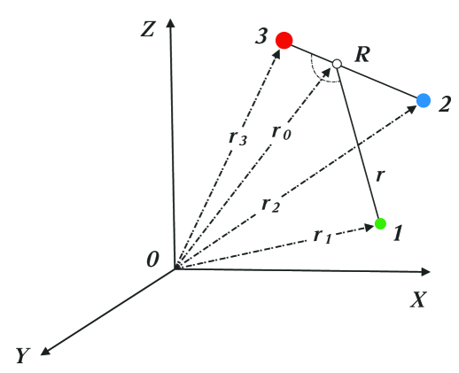
Figure 1: The Cartesian coordinate system where the set of radius vectors $\textbf{\emph{r}}_{1},\textbf{\emph{r}}_{2}$ and $\textbf{\emph{r}}_{3}$ denote positions of the 1, 2 and 3 bodies, respectively. The circle $"\circ"$ denotes the center of mass of pair (23) which in the Cartesian system is denoted by $\textbf{\emph{r}}_{0}$. The radius vectors R and r determine the Jacobi coordinate system, and $\theta$ denotes the scattering angle.

The three-body Hamiltonian (1), after the Jacobi coordinate transformations Delves1 acquires the form:

$$\breve{H}=\sum_{i=1}^{3}\frac{\textbf{P}^{2}_{i}}{2\mu_{i}}+\breve{V}\bigl{(}||\emph{{r}}-\lambda_{-}\emph{{R}}||,||\emph{{R}}||,||\emph{{r}}+\lambda_{+}\emph{{R}}||\bigr{)},$$ (3)

where the radius vector R denotes the relative displacement between 2 and 3 bodies (see FIG. 1), ${\textbf{\emph{r}}}=\emph{{r}}_{1}-\emph{{r}}_{0}$ is the relative displacement between the particle 1 and center of mass of the pair of particles (2, 3), while $\emph{{r}}_{0}=(m_{2}\emph{{r}}_{2}+m_{3}\emph{{r}}_{3})/(m_{1}+m_{2})$ is the radius vector of the center of mass of the pair (2, 3). In addition, the following notations are made in the equation (3) (see also AshGev ):

$$\textbf{P}_{1}=\emph{{p}}_{1}+\emph{{p}}_{2}+\emph{{p}}_{3},\quad\textbf{P}_{2}=\frac{m_{3}\emph{{p}}_{2}-m_{2}\emph{{p}}_{3}}{m_{2}+m_{3}},\quad\textbf{P}_{3}=\frac{(m_{2}+m_{3})\emph{{p}}_{1}-m_{1}(\emph{{p}}_{2}+\emph{{p}}_{3})}{\mu_{1}},$$

$$\mu_{1}=m_{1}+m_{2}+m_{3},\quad\mu_{2}=\frac{m_{2}m_{3}}{m_{2}+m_{3}},\quad\mu_{3}=\frac{m_{1}(m_{2}+m_{3})}{\mu_{1}},\quad\lambda_{-}=\frac{\mu_{2}}{m_{2}},\quad\lambda_{+}=\frac{\mu_{2}}{m_{3}}.$$

Removing the motion of the center of mass of the three-body system, that is equivalent to the condition $\textbf{P}_{1}=0$, leads the equation (3) to the form (see gev1 ):

$$\tilde{H}=\frac{1}{2\mu_{0}}\Bigl{(}\tilde{\textbf{P}}^{2}_{2}+\tilde{\textbf{P}}^{2}_{3}\Bigr{)}+\breve{V}\bigl{(}||\emph{{r}}-\lambda_{-}\emph{{R}}||,||\emph{{R}}||,||\emph{{r}}+\lambda_{+}\emph{{R}}||\bigr{)}.$$ (4)

In the equation (4) the following notations are made:

$$\mu_{0}=\Bigl{(}\frac{m_{1}m_{2}m_{3}}{\mu_{1}}\Bigr{)}^{1/2},\qquad\tilde{\textbf{P}}_{2}=\sqrt{\mu_{2}\mu_{0}}\dot{\emph{{R}}},\qquad\tilde{\textbf{P}}_{3}=\sqrt{\mu_{3}\mu_{0}}\dot{\emph{{r}}},$$

where $\dot{\emph{{x}}}=d\emph{{x}}/dt$ and $\emph{{x}}=(\emph{{R}},\emph{{r}}).$

Finally, the Hamiltonian (4) can be written as:

$$\mathbb{H}(\textbf{r},\textbf{p})=\frac{1}{2\mu_{0}}{\textbf{p}}^{2}+\mathbb{V}(\textbf{r}),$$ (5)

where $\mathbb{V}(\textbf{r})=\breve{V}\bigl{(}||\emph{{r}}-\lambda_{-}\emph{{R}}||,||\emph{{R}}||,||\emph{{r}}+\lambda_{+}\emph{{R}}||\bigr{)}$.
Note that (5) can be interpreted as a single-particle Hamiltonian with effective mass $\mu_{0}$ in a $12D$ phase space. In addition (5) the following notations are made:

$$\textbf{r}=\textbf{\emph{r}}\oplus{\textbf{\emph{R}}}\in{\mathbb{R}}^{6},\qquad\textbf{p}=\tilde{\textbf{\emph{P}}}_{2}\oplus\tilde{{\textbf{\emph{P}}}}_{3}\in{\mathbb{R}^{\ast}}^{6},$$ (6)

where $"\oplus"$ denotes the direct sum of the $3D$ vectors and, accordingly, r and p are the radius vector and the momentum of an imaginary point in the $6D$ configuration space. It is obvious that; $\mathbb{V}:\mathbb{R}^{3}\to\mathbb{R}^{1}$ and $\mathbb{H}:\mathbb{R}^{12}\to\mathbb{R}^{1}$.

Let us consider the following system of hyper-spherical coordinates:

$$\rho_{1}=r=||\textbf{\emph{r}}||,\quad\rho_{2}=R=||\textbf{\emph{R}}||,\quad\rho_{3}=\theta,\quad\rho_{4}=\Theta,\quad\rho_{5}=\Phi,\quad\rho_{6}=\Omega,$$ (7)

where the first set of three coordinates (coordinates of the internal space or the internal coordinates) $\{\bar{\rho}\}=(\rho_{1},\rho_{2},\rho_{3})$ determines the position of the effective mass $\mu_{0}$ (imaginary point) on the plane formed by three bodies. Note that the domain of definition of these coordinates, respectively, are $(\rho_{1},\rho_{2})\in[0,\infty]$ and $\theta\in[0,\pi].$ The set of coordinates $\{\underline{\rho}\}=(\Theta,\Phi,\Omega)$ will be called external coordinates. The domain of definition of these coordinates, respectively, are $\Theta\in(-\pi,+\pi]$,  $\Phi=(-\pi,+\pi]$ and $\Omega\in[0,\pi]$. Note that the external coordinates are the Euler angles describing the rotation of the plane in $3D$ space.

As was shown Klar ; Johonson ; Johonson1 ; Smor ; Kup ; Schatz ; Vinit ; Gusev , it is convenient to represent the motion of a three-body system as translational and rotational motion of a three-body triangle $\triangle(1,2,3)$, and also deformation of sides of the same triangle gev ; gev1 ; gev0 . In particular, the kinetic energy in this case can be written in the form Fiz :

$$T=\frac{\mu_{0}}{2}\bigl{\{}\dot{{\textbf{\emph{R}}}}^{2}+\dot{{\textbf{\emph{r}}}}^{2}\bigr{\}}=\frac{\mu_{0}}{2}\Bigl{\{}\dot{\emph{R}}^{2}+{\emph{R}}^{2}\bigl{[}\bm{\omega}\times\textbf{k}\bigr{]}^{2}+\bigl{(}\dot{{\textbf{\emph{r}}}}+[\bm{\omega}\times{\textbf{\emph{r}}}]\bigr{)}^{2}\Bigr{\}},$$ (8)

where the direction of the unit vector k in the moving reference frame $\{\rho\}$ is determined by the expression ${\emph{{R}}}{||\emph{{R}}||}^{-1}=\pm\textbf{k}$. Below we will assume that the vector $\textbf{k}=(0,0,1)$ is directed toward the positive direction of the axis $OZ$ (below will be designated as the axis $z$ ), and the angular velocity $\bm{\omega}$ describes the rotation of the frame $\{\bar{\rho}\}$ relative to the laboratory system.

Having carried out simple calculations in the expression (8) it is easy to find:

$$T=\frac{\mu_{0}}{2}\Bigl{\{}\dot{{{\emph{R}}}}^{2}+\dot{{{\emph{r}}}}^{\,2}+r^{2}\dot{\theta}^{2}+A{{{\emph{R}}}}^{2}+B{{{\emph{r}}}}^{\,2}\Bigr{\}},$$ (9)

where the following notations are made:

$$A=\omega_{x}^{2}+\omega_{y}^{2},\qquad B=\omega^{2}_{y}+\bigl{(}\omega_{x}\cos\theta-\omega_{z}\sin\theta\bigr{)}^{2}.$$

Note that when deriving the expression (9) we used the definition of a moving system $\{\bar{\varrho}\}$, suggesting that the unit vector $\bm{\gamma}=\textbf{\emph{r}}||\textbf{\emph{r}}||^{-1}$ lies on the plane $OXZ$ at the angle $\theta$ relative to the axis $OZ$, that is; $\bm{\gamma}=(\sin\theta,0,\cos\theta)$. As for angular velocity projections, they satisfy the following equations:

$$\omega_{x}=\dot{\Phi}\sin\Theta\sin\Omega+\dot{\Theta}\cos\Omega,$$

$$\omega_{y}=\dot{\Phi}\sin\Theta\cos\Omega-\dot{\Theta}\sin\Omega,$$

$$\omega_{z}=\dot{\Phi}\cos\Theta-\dot{\Omega}.$$ (10)

Taking into account (9) and (10), the kinetic energy of the three-body system in Euclidean space can be written in the tensor form:

$$T=\frac{\mu_{0}}{2}\gamma^{\alpha\beta}\frac{d\rho_{\alpha}}{dt}\frac{d\rho_{\beta}}{dt},\qquad\alpha,\beta=(1,2,...,6)=\overline{1,6},$$

where $\gamma^{\alpha\beta}$ is the metric tensor, which has the form:

$$\gamma^{\alpha\beta}=\left(\begin{array}[]{cccccc}\gamma^{11}&\,0&0&0&\,0&\,0\\ 0&\gamma^{22}&\,0&0&\,0&\,0\\ 0&\,0&\gamma^{33}&0&\,0&\,0\\ 0&\,0&\,0&\gamma^{44}&\gamma^{45}&\gamma^{46}\\ 0&\,0&\,0&\gamma^{54}&\gamma^{55}&\gamma^{56}\\ 0&\,0&\,0&\gamma^{64}&\gamma^{65}&\gamma^{66}\\ \end{array}\right),$$ (11)

in addition, the following notations are made (see Appendix A):

$$\gamma^{11}=\gamma^{22}=1,\quad\gamma^{33}=r^{2},\quad\gamma^{44}=R^{2}+\,r^{2}\bigl{(}1\,-\sin^{2}\theta\cos^{2}\Omega\bigr{)},\quad\gamma^{55}\,=R^{2}\sin^{2}\Theta\,\,+$$

$$r^{2}\bigl{\{}\sin^{2}\Theta(1-\sin^{2}\theta\sin^{2}\Omega)+\sin^{2}\theta\cos^{2}\Theta+(1/2)\sin 2\theta\sin 2\Theta\sin\Omega\bigr{\}},\quad\gamma^{66}=r^{2}\sin^{2}\theta,$$

$$\gamma^{45}=\gamma^{54}\,=\,-(1/2)r^{2}\,\bigl{(}\sin^{2}\theta\sin\Theta\sin 2\Omega+\sin 2\theta\cos\Theta\cos\Omega\bigr{)},\quad\gamma^{46}=\gamma^{64}=(1/2)\,\times$$

$$r^{2}\sin 2\theta\cos\Omega,\qquad\gamma^{56}=\gamma^{65}=-(1/2)r^{2}\bigl{(}\sin 2\theta\sin\Theta\sin\Omega-2\sin^{2}\theta\cos\Theta\bigr{)}.$$

Using the metric tensor (11), one can write a linear infinitesimal element of Euclidean space in hyperspherical coordinates:

$$(ds)^{2}=\gamma^{\alpha\beta}(\{\rho\})d\rho_{\alpha}d\rho_{\beta},\qquad\alpha,\beta=\overline{1,6}.$$ (12)

Definition 2. Let $(F,G):\mathbb{R}^{12}\to\mathbb{R}^{1}$ be functions of 12 variables $(r_{\alpha},p_{\alpha}),$where $\alpha=\overline{1,6}.$ The Poisson bracket on the phase space $\mathcal{P}\cong\mathbb{R}^{12}$ is defined by the following form:

$$\{F,G\}=\sum_{\alpha=1}^{6}\biggl{(}\frac{\partial F}{\partial r_{\alpha}}\frac{\partial G}{\partial p_{\alpha}}-\frac{\partial F}{\partial p_{\alpha}}\frac{\partial G}{\partial r_{\alpha}}\biggr{)}.$$ (13)

Note that the variables $r_{\alpha}$ and $p_{\alpha}$ denote the projections of 6D radius vector $\textbf{r}\in\mathbb{R}^{6}$ and the momentum $\textbf{p}\in\mathbb{R}^{\ast 6},$ respectively (see equation (6), and also the Definition 1).

Definition 3. Let $\mathbb{H}:\mathbb{R}^{12}\to\mathbb{R}^{1}$ be the Hamiltonian of the imaginary point with the mass $\mu_{0}$ in the 12-dimensional phase space. The Hamiltonian vector field $\textbf{X}_{\mathbb{H}}:\mathbb{R}^{12}\to\mathbb{R}^{12}$ satisfies the equation:

$$\textbf{X}_{\mathbb{H}}(\textbf{z})=\{\textbf{z},\mathbb{H}\},\qquad\textbf{z}\in\mathbb{R}^{12}.$$ (14)

Definition 4. The Hamiltonian equations in the phase space $\mathcal{P}\cong\mathbb{R}^{12}$ will be defined as follows:

$$\dot{\textbf{z}}=\textbf{X}_{\mathbb{H}},\qquad\dot{\textbf{z}}=\frac{d\textbf{z}}{dt}\in\mathbb{R}^{12},$$ (15)

or, equivalently:

$$\dot{r}_{\alpha}=\frac{\partial\mathbb{H}}{\partial p_{\alpha}},\qquad\dot{p}_{\alpha}=-\frac{\partial\mathbb{H}}{\partial r_{\alpha}}.$$ (16)

Without going into well-known details, we note that the problem under consideration, having in the general case 10 independent integrals of motion, reduces to the system of 8th order. In the case when the total energy is fixed, the reduction of the problem leads to the system of 7th order system (see Whitt , and also Chen ).

Note that only in very few specific cases, the problem of the gravity of three bodies is exactly integrated.

III Three-body problem as a problem of geodesic flows on Riemannian manifold

The classical three-body system moving in the Euclidean $3D$ space continuously forms a triangle, and, therefore, Newton’s equations describe a dynamical system on the space of such triangles Fiz . The latter means that we can formally divide the motion into two parts, the first of which is the rotational motion of the triangle of bodies in $3D$ Euclidean space, and the second is the internal motion of bodies in the plane of the triangle.

As well-known, the configuration space of the solid body $\mathbb{R}^{6}$ can be represented as a direct product of two subspaces Arnold1 :

$$\mathbb{R}^{6}:\Leftrightarrow\mathbb{R}^{3}\times\mathbb{S}^{3},$$ (17)

where $:\Leftrightarrow$ by definition denotes equivalence, ${\mathbb{R}}^{3}$ is a manifold that is defined as the orthonormal space of relative distances between bodies, and $\mathbb{S}^{3}$ denotes the space of the rotation group $SO(3)$. Note that in the considered problem the connections between the bodies are not holonomic, and therefore the representation (17) for the configuration space is incorrect.

Definition 5. Let $\mathcal{M}$ be a 6D Riemannian manifold on which the local coordinate system is defined:

$$\overline{x^{1},x^{6}}=\{x\}=(x^{1},...,x^{6})\in\mathcal{M},$$ (18)

where the set $\{\bar{x}\}=(x^{1},x^{2},x^{3})$ will be called the internal coordinates, and the set $\{\underline{x}\}=(x^{4},x^{5},x^{6})$, respectively, the external coordinates.
It is assumed that $\mathcal{M}$ is a conformal-Euclidean manifold or Weyl space (see Nord ) immersed in the Euclidean space $\mathbb{R}^{6}$, which is determined by the metric tensor:

$$g_{\mu\nu}(\{\bar{x}\})=g(\{\bar{x}\})\delta_{\mu\nu},\qquad g(\{\bar{x}\})=\bigl{[}\mathrm{E}-U(\{\bar{x}\})\bigr{]}U^{-1}_{0}\neq 0,\qquad\mu,\nu=\overline{1,6},$$ (19)

where $\delta_{\mu\nu}$ denotes the Kronecker symbol, $\mathrm{E}$ is the total energy of three-body system, $U(\{\bar{x}\})$ is the total interaction potential between bodies and $U_{0}=max|U(\{\bar{x}\})|$.

Proposition 1. If 6D manifold $\mathcal{M}$ is described by the metric tensor (19), then it can be represented as a direct product of two subspaces:

$$\mathcal{M}:\Leftrightarrow\mathcal{M}^{(3)}\times\mathcal{S}^{3}_{M_{k}}.$$ (20)

where $\mathcal{M}^{(3)}$ denotes $3D$ Riemannian manifold defined as follows:

$$\mathcal{M}^{(3)}=\bigl{[}\{\bar{x}\}=(x^{1},x^{2},x^{3})\in\mathcal{M}^{(3)}_{t};\,g_{ij}(\{\bar{x}\})=g(\{\bar{x}\})\delta_{ij};\,\,g(\{\bar{x}\})\neq 0\bigr{]}.$$

In addition, $\mathcal{M}^{(3)}_{t}\cong\bigcup_{k}M_{k}$ denotes the atlas of the manifold $\mathcal{M}^{(3)}$ (internal space) and $M_{k}\ni(x^{1},x^{2},x^{3})_{k}$ is the $k$-$th$ card. Note that the atlas $\mathcal{M}^{(3)}_{t}$, immersed in the manifold $\mathcal{M}$, is invariant under the local rotations group $SO(3)_{M_{k}}$ (external space $\mathcal{S}_{M_{k}}^{3}\ni(x^{4},x^{5},x^{6})_{M_{k}}$).
Proof.

Using the Maupertuis’ variational principle, one can derive equations for geodesic trajectories on the Riemannian manifold $\mathcal{M}$ (see Arnold1 ; BubrNovFom ):

$$\ddot{x}^{\mu}+\Gamma^{\mu}_{\nu\gamma}(\{\bar{x}\})\dot{x}^{\,\nu}\dot{x}^{\,\gamma}=0,\qquad\mu,\nu,\gamma=\overline{1,6},$$ (21)

where

$$\dot{x}^{\,\mu}=\frac{dx^{\mu}}{ds},\qquad\ddot{x}^{\,\mu}=\frac{d^{\,2}x^{\mu}}{ds^{2}},\qquad s=\int\sqrt{g_{\mu\nu}(\{\bar{x}\})dx^{\mu}dx^{\nu}}.$$ (22)

Recall that $\dot{x}^{\mu}$ and $\ddot{x}^{\,\mu}$ denote the geodesic velocity and acceleration, respectively, while $``s"$ denotes the length of a curve along a geodesic trajectory. Note that it plays the role of a chronological parameter, which orders the sequence of stages of the dynamical system motion, and in further will be called internal time of the system. In the equations (21) $\Gamma^{\mu}_{\nu\gamma}(\{x\})$ denotes the Christoffel symbol:

$$\Gamma^{\mu}_{\nu\gamma}(\{\bar{x}\})=\frac{1}{2}g^{\mu\mu}\bigl{(}{\partial_{\gamma}g_{\mu\nu}}+\partial_{\nu}g_{\gamma\mu}-\partial_{\mu}g_{\nu\gamma}\bigr{)},\qquad\partial_{\mu}\equiv\partial_{x^{\mu}}.$$

Taking into account (19) and (21), one can obtain the following equations for geodesic trajectories:

$$\ddot{x}^{1}=a_{1}\Bigl{\{}\bigl{(}\dot{x}^{1}\bigr{)}^{2}-\sum_{\mu\neq 1,\,\mu=2}^{6}\bigl{(}\dot{x}^{\mu}\bigr{)}^{2}\Bigr{\}}+2\dot{x}^{1}\Bigl{\{}a_{2}\dot{x}^{2}+a_{3}\dot{x}^{3}\Bigr{\}},$$

$$\ddot{x}^{2}=a_{2}\Bigl{\{}\bigl{(}\dot{x}^{\,2}\bigr{)}^{2}-\sum_{\mu=1,\,\mu\neq 2}^{6}\bigl{(}\dot{x}^{\mu}\bigr{)}^{2}\Bigr{\}}+2\dot{x}^{2}\Bigl{\{}a_{3}\dot{x}^{3}+a_{1}\dot{x}^{1}\Bigr{\}},$$

$$\ddot{x}^{3}=a_{3}\Bigl{\{}\bigl{(}\dot{x}^{3}\bigr{)}^{2}-\sum_{\mu=1,\,\mu\neq 3}^{6}\bigl{(}\dot{x}^{\mu}\bigr{)}^{2}\Bigr{\}}+2\dot{x}^{3}\Bigl{\{}a_{1}\dot{x}^{1}+a_{2}\dot{x}^{2}\Bigr{\}},$$

$$\qquad\qquad\qquad\qquad\quad\,\ddot{x}^{4}=2\dot{x}^{4}\Bigl{\{}a_{1}\dot{x}^{1}+a_{2}\dot{x}^{2}+a_{3}\dot{x}^{3}\Bigr{\}},$$

$$\ddot{x}^{5}=2\dot{x}^{5}\Bigl{\{}a_{1}\dot{x}^{1}+a_{2}\dot{x}^{2}+a_{3}\dot{x}^{3}\Bigr{\}},$$

$$\ddot{x}^{6}=2\dot{x}^{6}\Bigl{\{}a_{1}\dot{x}^{1}+a_{2}\dot{x}^{2}+a_{3}\dot{x}^{3}\Bigr{\}},$$ (23)

where

$$a_{i}(\{\bar{x}\})=-\partial_{x^{i}}\ln\sqrt{g(\{\bar{x}\})},\qquad\partial_{x^{i}}\equiv\partial/\partial x^{i},$$ (24)

in addition, the metric $g_{\mu\nu}$ is the conformal-Euclidean and, therefore, $g(\{\bar{x}\})=g_{11}(\{\bar{x}\})=...=g_{66}(\{\bar{x}\})$.

It is easy to show that in the system (23) the last three equations can be exactly integrated:

$$\dot{x}^{\mu}=J_{\mu-3}/g(\{\bar{x}\}),\quad J_{\mu-3}=const_{\mu-3},$$ (25)

where $\mu=\overline{4,6}.$

Note that $J_{1},J_{2}$ and $J_{3}$ are integrals of the motion of the problem. They can be interpreted as projections of the total angular momentum of the three-body system $J=\sqrt{\sum_{i=1}^{3}J^{2}_{i}}=const$ on the corresponding three orthogonal local axes $\bigl{(}x^{1},x^{2},x^{3}\bigr{)}$. Recall that for the classical problem these projections can continuously change and take arbitrary values.

Substituting (25) into the equations (23), we obtain the following system of second-order nonlinear ordinary differential equations:

$$\ddot{x}^{1}=a_{1}\bigl{\{}(\dot{x}^{1})^{2}-(\dot{x}^{2})^{2}-(\dot{x}^{3})^{2}-\Lambda^{2}\bigr{\}}+2\dot{x}^{1}\bigl{\{}a_{2}\dot{x}^{2}+a_{3}\dot{x}^{3}\bigr{\}},$$

$$\ddot{x}^{2}=a_{2}\bigl{\{}(\dot{x}^{2})^{2}-(\dot{x}^{3})^{2}-(\dot{x}^{1})^{2}-\Lambda^{2}\bigr{\}}+2\dot{x}^{2}\bigl{\{}a_{3}\dot{x}^{3}+a_{1}\dot{x}^{1}\bigr{\}},$$

$$\ddot{x}^{3}=a_{3}\bigl{\{}(\dot{x}^{3})^{2}-(\dot{x}^{1})^{2}-(\dot{x}^{2})^{2}-\Lambda^{2}\bigr{\}}+2\dot{x}^{3}\bigl{\{}a_{1}\dot{x}^{1}+a_{2}\dot{x}^{2}\bigr{\}},\,$$ (26)

where $a_{i}\equiv a_{i}(\{\bar{x}\})$ and $\Lambda^{2}\equiv\Lambda^{2}(\{\bar{x}\})=\bigl{(}J/g(\{\bar{x}\})\bigr{)}^{2}.$

The system of equations (26) describes motion of geodesic flows on an oriented $3D$ submanifold $\mathcal{M}^{(3)}_{\{\bar{J}\}}\,$(the set of projections $\{\bar{J}\}=(J_{1},J_{2},J_{3})$ defines the submanifold orientation), which is immersed in the $6D$ manifold (space) $\mathcal{M}$.

The system of equations (26) can be represented as a 6th order system, that is, a system consisting of six first order differential equations:

$$\dot{\xi^{1}}=a_{1}\bigl{\{}(\xi^{1})^{2}-(\xi^{2})^{2}-(\xi^{3})^{2}-\Lambda^{2}\bigr{\}}+2\xi^{1}\bigl{\{}a_{2}\xi^{2}+a_{3}\xi^{3}\bigr{\}},\qquad\xi^{1}=\dot{x}^{1},$$

$$\dot{\xi}^{2}=a_{2}\bigl{\{}(\xi^{2})^{2}-(\xi^{3})^{2}-(\xi^{1})^{2}-\Lambda^{2}\bigr{\}}+2\xi^{2}\bigl{\{}a_{3}\xi^{3}+a_{1}\xi^{1}\bigr{\}},\qquad\xi^{2}=\dot{x}^{2},$$

$$\dot{\xi}^{3}=a_{3}\bigl{\{}(\xi^{3})^{2}-(\xi^{1})^{2}-(\xi^{2})^{2}-\Lambda^{2}\bigr{\}}+2\xi^{3}\bigl{\{}a_{1}\xi^{1}+a_{2}\xi^{2}\bigr{\}},\,\qquad\xi^{3}=\dot{x}^{3}.$$ (27)

Thus, we proved that the last three equations in (23) describing the external three coordinates $\{\underline{x}\}$ are exactly integrated and form a local rotation group $SO(3)_{M_{i}}$. The latter means that the 6$D$ manifold $\mathcal{M}$ can be continuously filled with the submanifold $\mathcal{M}^{(3)}_{\{\bar{J}\}}$, rotating it according to the law of the local symmetry group $SO(3)_{M_{i}}$ and therefore the representation (20) is true.

Proposition 1 is proved.

III.1 Reduced Hamiltonian in the internal space $\mathbb{E}^{3}\subset\mathbb{R}^{3}$

Taking into account (19) and (25), we can reduce the Hamiltonian and obtain the following representation for it:

$$\mathcal{H}\bigl{(}\{\bar{x}\};\{\bar{p}\}\bigr{)}=\frac{1}{2\mu_{0}}g^{\mu\nu}(\{\bar{x}\}p_{\mu}p_{\nu}=\frac{1}{2\mu_{0}g(\{\bar{x}\})}p_{\mu}p_{\nu}\delta^{\mu\nu}\,\,\,\,$$

$$=\frac{1}{2}\mu_{0}g(\{\bar{x}\})\Biggl{\{}\sum_{i=1}^{3}\bigl{(}\dot{x}^{i}\bigr{)}^{2}\,+\,\biggl{(}\frac{J}{g(\{\bar{x}\})}\biggr{)}^{2}\Biggr{\}},$$ (28)

where $\{\bar{p}\}=(p_{\,1},p_{\,2},p_{\,3})$ and $\mu,\nu=\overline{1,6}.$
Note that the reduced Hamiltonian (28) is clearly independent of the mass of the bodies. If we analyze the stages of obtaining the expression (28), we will see that the representation contains a dependence on the masses, however it is hidden in coordinate transformations (see transformations above (3)). The system of geodesic equations (26) can be obtained using the Hamilton equations:

$$\dot{x}^{i}=\frac{\partial\mathcal{H}}{\partial p_{i}}=g^{ik}(\{\bar{x}\})p_{k},\qquad\dot{p}_{i}=-\frac{\partial\mathcal{H}}{\partial x^{i}}=-\frac{1}{2\mu_{0}}\frac{\partial g^{kl}(\{\bar{x}\})}{\partial x^{i}}p_{k}p_{l},$$ (29)

where $i,k,l=\overline{1,3}$.

Finally, assuming that in the three-body system the total energy is fixed:

$$\mathrm{E}=\mathcal{H}\bigl{(}\{\bar{x}\};\{\bar{p}\}\bigr{)}=const,$$ (30)

the problem can be reduced to the 5th order system.

Thus, the system of equations (27) is the 6th order system, which describes the dynamics of an imaginary point with an effective mass $\mu_{0}$ on the 3D Riemannian manifold $\mathcal{M}^{(3)}_{\{\bar{J}\}}$. Note that the system of equations (27) can also be obtained from the Hamilton equations (29) using the reduced Hamiltonian (28). Using the system of equations (27), we can study in detail the behavior of geodesic flows of various elementary atom-molecular processes in the internal space $\mathbb{E}^{3}\subset\mathbb{R}^{3}$.

IV The mappings between 6D Euclidean and 6D conformal-Euclidean subspaces

Now the main problem is to prove that the 6th order system (27) is equivalent to the original three-particle Newtonian problem (16). Recall, that both representations will be equivalent, if we prove that there exists continuous one-to-one mappings between the two following manifolds $\mathbb{E}^{6}$ and $\mathcal{M}$, where $\mathbb{E}^{6}\subset\mathbb{R}^{6}$ is a subspace allocated from the Euclidean space $\mathbb{R}^{6}$ taking into account the condition:

$$\breve{g}(\{\bar{\rho}\})=\mathrm{E}-\mathbb{V}(\{\bar{\rho}\})\neq 0.$$ (31)

In other words, we must prove that between two sets of coordinates $\overline{\rho^{1},\rho^{6}}=\{\rho\}\in\mathbb{E}^{6}$ and $\overline{x^{1},x^{6}}=\{x\}\in\mathcal{M}$, there are continuous direct and inverse one-to-one mappings.

In this regard, it makes sense to consider three cases:

a. When $\breve{g}(\{\bar{\rho}\})<0$, the system of equations (27) obviously describes a restricted three-body problem.

b. When $\breve{g}(\{\bar{\rho}\})>0$, we are dealing with a typical scattering problem in a three-body system.

c. When $\breve{g}(\{\bar{\rho}\})=0$. This is a special and very important case, which, generally speaking, requires an extension of the Maupertuis-Hamilton principle of least action on the case of complex-classical trajectories. In this article, we will touch upon this problem problem when considering a restricted three-body problem.

IV.1 On a homeomorphism between the subspace $\mathbb{E}^{6}\subset\mathbb{R}^{6}$ and the manifold $\mathcal{M}$

Proposition 2. If the interaction potential between the three bodies has the form (2) and, moreover, it belongs to the class $\mathbb{V}(\{\bar{\rho}\})\in\mathbb{C}^{1}(\mathbb{R}^{6})$, then the Euclidean subspace $\mathbb{E}^{6}\subset\mathbb{R}^{6}$ is homeomorphic to the manifold $\mathcal{M}$.
Proof.

Let us consider a linear infinitesimal element $(ds)$ in both coordinate systems $\{\rho\}\in\mathbb{E}^{6}$ and $\{x\}\in\mathcal{M}$. Equating them, we can write:

$$(ds)^{2}=\gamma^{\alpha\beta}(\{\mathrm{\rho}\})d\mathrm{\rho}_{\alpha}d\mathrm{\rho}_{\beta}=g_{\mu\nu}(\{\bar{x}\})dx^{\mu}{dx^{\nu}},\quad\alpha,\beta,\mu,\nu=\overline{1,6},$$ (32)

from which one can obtain the following system of algebraic equations:

$$\gamma^{\alpha\beta}(\{\mathrm{\rho}\})\rho_{\alpha,\mu}\rho_{\beta,\nu}=g_{\mu\nu}(\{\bar{x}\})=g(\{\bar{x}\})\delta_{\mu\nu},$$ (33)

where it is necessary to prove that the coefficients $\mathrm{\rho}_{\alpha,\mu}(\{x\})=\partial\mathrm{\rho}_{\alpha}/\partial{x}^{\mu}$ have the meaning of derivatives. In this regard, we must prove that the function $\mathrm{\rho}_{\alpha}(\{x\})$ is twice differentiable and continuous in the whole domain of its definition and satisfy the symmetry condition:

$$\mathrm{\rho}_{\alpha,\mu\nu}(\{x\})=\mathrm{\rho}_{\alpha,\nu\mu}(\{x\}),\qquad\qquad\forall\,\,\mu,\nu=\overline{1,6},$$ (34)

(Schwartz’s theorem on the symmetry of second derivatives).

Recall that the set of coefficients $\mathrm{\rho}_{\alpha,\mu}(\{x\})$ allows us to perform coordinate transformations $\{\rho\}\mapsto\{x\}$, which we shall call direct transformations.

Similarly, from (32), one can obtain a system of algebraic equations defining inverse transformations:

$$\gamma_{\alpha\beta}(\{\rho\})g^{-1}(\{\bar{x}\})=x^{\mu}_{\,\,,\,\alpha}x^{\nu}_{\,\,,\,\beta}\,\delta_{\mu\nu},$$ (35)

where $x^{\mu}_{\,\,,\,\alpha}(\{\rho\})=\partial x^{\mu}/\partial{\rho}^{\alpha}$ and $\gamma_{\alpha\beta}(\{{\rho}\})=\gamma_{\alpha\bar{\alpha}}(\{{\rho}\})\,\gamma_{\beta\bar{\beta}}(\{{\rho}\})\,\gamma^{\bar{\alpha}\bar{\beta}}(\{{\rho}\})$.

At first we consider the system of equations (33), which is related to direct coordinate transformations. It is not difficult to see that the system of algebraic equations (33) is underdetermined with respect to the variables $\mathrm{\rho}_{\alpha,\mu}(\{x\})$, since it consists of 21 equations, while the number of unknown variables is 36. Obviously, when these equations are compatible, then the system of equations (33) has an infinite number of real and complex solutions. Note that for the classical three-body problem, the real solutions of the system (33) are important, which form a 15 -dimensional manifold. Since the system of equations (35) is still defined in a rather arbitrary way we can impose additional conditions on it in order to find the minimal dimension of the manifold allowing a separation of the base $\mathcal{M}^{(3)}_{\{\bar{J}\}}$ from the layer $\bigcup_{i}\mathcal{S}^{3}_{M_{i}}$ (see expression (20)).

Let us make a new notations:

$$\alpha_{\mu}=\rho_{1,\mu},\quad\beta_{\mu}=\rho_{2,\mu},\quad\zeta_{\mu}=\rho_{3,\mu},\quad u_{\mu}=\rho_{4,\mu},\quad v_{\mu}=\rho_{5,\mu},\quad w_{\mu}=\rho_{6,\mu}.$$ (36)

We also require that the following additional conditions be met:

$$\alpha_{4}=\alpha_{5}=\alpha_{6}=0,\qquad\beta_{4}=\beta_{5}=\beta_{6}=0,\qquad\zeta_{4}=\zeta_{5}=\,\zeta_{6}\,=0,$$

$$u_{1}=u_{2}=u_{3}=0,\qquad v_{1}=v_{2}=v_{3}=0,\qquad w_{1}=w_{2}=w_{3}=0.$$ (37)

Using (11), (36) and conditions (37) from the equation (33) we can obtain two independent systems of algebraic equations:

$$\alpha_{1}^{2}+\beta_{1}^{2}+\gamma^{33}\zeta_{1}^{2}\,=\,\breve{g}(\{\bar{\rho}\}),\qquad\alpha_{1}\alpha_{2}+\beta_{1}\beta_{2}+\gamma^{33}\zeta_{1}\zeta_{2}=0,$$

$$\alpha_{2}^{2}+\beta_{2}^{2}+\gamma^{33}\zeta_{2}^{2}\,=\,\breve{g}(\{\bar{\rho}\}),\qquad\alpha_{1}\alpha_{3}+\beta_{1}\beta_{3}+\gamma^{33}\zeta_{1}\zeta_{3}=0,$$

$$\alpha_{3}^{2}+\beta_{3}^{2}+\gamma^{33}\zeta_{3}^{2}\,=\,\breve{g}(\{\bar{\rho}\}),\qquad\alpha_{2}\alpha_{3}+\beta_{2}\beta_{3}+\gamma^{33}\zeta_{2}\zeta_{3}=0,$$ (38)

and, correspondingly:

$$\gamma^{44}u_{4}^{2}+\gamma^{55}v_{4}^{2}+\gamma^{66}w_{4}^{2}+2(\gamma^{45}u_{4}v_{4}+\gamma^{46}u_{4}w_{4}+\gamma^{56}v_{4}w_{4})=\breve{g}(\{\bar{\rho}\}),$$

$$\gamma^{44}u_{5}^{2}+\gamma^{55}v_{5}^{2}+\gamma^{66}w_{5}^{2}+2(\gamma^{45}u_{5}v_{5}+\gamma^{46}u_{5}w_{5}+\gamma^{56}v_{5}w_{5})=\breve{g}(\{\bar{\rho}\}),$$

$$\gamma^{44}u_{6}^{2}+\gamma^{55}v_{6}^{2}+\gamma^{66}w_{6}^{2}+2(\gamma^{45}u_{6}v_{6}+\gamma^{46}u_{6}w_{6}+\gamma^{56}v_{6}w_{6})=\breve{g}(\{\bar{\rho}\}),$$

$$a_{4}u_{4}+a_{5}v_{4}+a_{6}w_{4}=0,$$

$$b_{4}u_{5}+b_{5}v_{5}+b_{6}w_{5}=0,$$

$$c_{4}u_{6}+c_{5}v_{6}+c_{6}w_{6}=0.$$ (39)

In equations (39) the following notations are made:

$$a_{i}=\gamma^{i4}u_{5}+\gamma^{i5}v_{5}+\gamma^{i6}w_{5},\quad b_{j}=\gamma^{j4}u_{6}+\gamma^{j5}v_{6}+\gamma^{j6}w_{6},\quad c_{k}=\gamma^{k4}u_{4}+\gamma^{k5}v_{4}+\gamma^{k6}w_{4},$$

where $i,j,k=\overline{4,6}.$

It should be noted that the solutions of algebraic systems (38) and (39) form two different 3$D$ manifolds $\mathfrak{S}^{(3)}$ and $\mathfrak{R}^{(3)}$, respectively. Since the manifold $\mathfrak{S}^{(3)}$ play a key role in the proofs and the theoretical constructions of representation, the features of its structure are studied in detail (see Appendix B). Note that the manifold $\mathfrak{S}^{(3)}$ is in a one-to-one mapping on the one hand with the subspace $\mathbb{E}^{3}\ni\{\bar{\rho}\}$ (where $\mathbb{E}^{3}\subset\mathbb{E}^{6}$ the internal space in the hyperspherical coordinate system), and on the other hand with the submanifold $\mathcal{M}^{(3)}_{\{\bar{J}\}}$ (see FIG. 2). Note that this statement follows from the fact that all points of the submanifold $\mathcal{M}^{(3)}_{\{\bar{J}\}}$ and the subspace $\mathbb{E}^{3}\subset\mathbb{R}^{3}$, are pairwise connected through the corresponding derivatives (see (33)), which, as unknown variables, enter the algebraic equations (38), and, in addition, as shown there exist also inverse coordinate transformations (see Appendix C).

Now we prove continuity of these mappings. Recall that the unknowns in the equations (38) are in fact functions of coordinates $\{\bar{\rho}\}$. By making infinitely small coordinate shifts $\{\bar{\rho}\}\to\{\bar{\rho}\}+\{\delta\bar{\rho}\}$ in (38), we get the following system of equations:

$$\bar{\alpha}_{1}^{2}+\bar{\beta}_{1}^{2}+\bar{\gamma}^{33}\bar{\zeta}_{1}^{2}=\bar{g}(\{\bar{\rho}\}),\qquad\bar{\alpha}_{1}\bar{\alpha}_{2}+\bar{\beta}_{1}\bar{\beta}_{2}+\bar{\gamma}^{33}\bar{\zeta}_{1}\bar{\zeta}_{2}=0,$$

$$\bar{\alpha}_{2}^{2}+\bar{\beta}_{2}^{2}+\bar{\gamma}^{33}\bar{\zeta}_{2}^{2}=\bar{g}(\{\bar{\rho}\}),\qquad\bar{\alpha}_{1}\bar{\alpha}_{3}+\bar{\beta}_{1}\bar{\beta}_{3}+\bar{\gamma}^{33}\bar{\zeta}_{1}\bar{\zeta}_{3}=0,$$

$$\bar{\alpha}_{3}^{2}+\bar{\beta}_{3}^{2}+\bar{\gamma}^{33}\bar{\zeta}_{3}^{2}=\bar{g}(\{\bar{\rho}\}),\qquad\bar{\alpha}_{2}\bar{\alpha}_{3}+\bar{\beta}_{2}\bar{\beta}_{3}+\bar{\gamma}^{33}\bar{\zeta}_{2}\bar{\zeta}_{3}=0,$$ (40)

where

$$\bar{g}(\{\bar{\rho}\})=\breve{g}\bigl{(}\{\bar{\rho}\}+\{\delta\bar{\rho}\}\bigr{)},\qquad\{\delta\bar{\rho}\}=(\delta\rho^{1},\delta\rho^{2},\delta\rho^{3}).$$

Assuming that the displacement $||\,\delta\{\bar{\rho}\}||\ll 1$, in the equations (40), we can expand the functions in a Taylor series, and further, taking into account the equations system (38), we can get:

$$\delta\rho^{i}\bigl{\{}2(\alpha_{1}\alpha_{1\,i}+\beta_{1}\beta_{1\,i}+\gamma^{33}\zeta_{1}\zeta_{1\,i})+\gamma^{33}_{,\,i}\zeta_{1}^{2}-\breve{g}_{,\,i}(\{\bar{\rho}\})\bigr{\}}+O(||\,\delta\{\bar{\rho}\}||^{2})=0,\,\,\,$$

$$\delta\rho^{i}\bigl{\{}2(\alpha_{2}\alpha_{2\,i}+\beta_{2}\beta_{2\,i}+\gamma^{33}\zeta_{2}\zeta_{2\,i})+\gamma^{33}_{,\,i}\zeta_{2}^{2}-\breve{g}_{,\,i}(\{\bar{\rho}\})\bigr{\}}+O(||\delta\{\bar{\rho}\}||^{2})=0,\,\,\,$$

$$\delta\rho^{i}\bigl{\{}2(\alpha_{3}\alpha_{3\,i}+\beta_{3}\beta_{3\,i}+\gamma^{33}\zeta_{3}\zeta_{3,i})+\gamma^{33}_{,\,i}\zeta_{3}^{2}-\breve{g}_{,\,i}(\{\bar{\rho}\})\bigr{\}}\,+\,O(||\delta\{\bar{\rho}\}||^{2})=0,\,\,\,$$

$$\delta\rho^{i}\bigl{\{}{\alpha}_{1}{\alpha}_{2\,i}+{\alpha}_{2}{\alpha}_{1\,i}+{\beta}_{1}{\beta}_{2\,i}+{\beta}_{2}{\beta}_{1\,i}+\gamma^{33}({\zeta}_{1}{\zeta}_{2\,i}+{\zeta}_{2}{\zeta}_{1\,i})+{\gamma}^{33}_{,\,i}{\zeta}_{1}{\zeta}_{2}\bigl{\}}+O(||\,\delta\{\bar{\rho}\}||^{2})=0,\,\,\,$$

$$\delta\rho^{i}\bigl{\{}{\alpha}_{1}{\alpha}_{3\,i}+{\alpha}_{3}{\alpha}_{1\,i}+{\beta}_{1}{\beta}_{3\,i}+{\beta}_{3}{\beta}_{1\,i}+\gamma^{33}({\zeta}_{1}{\zeta}_{3\,i}+{\zeta}_{3}{\zeta}_{1\,i})+{\gamma}^{33}_{,\,i}{\zeta}_{1}{\zeta}_{3}\bigl{\}}+O(||\,\delta\{\bar{\rho}\}||^{2})=0,\,\,\,$$

$$\delta\rho^{i}\bigl{\{}{\alpha}_{2}{\alpha}_{3,\,i}+{\alpha}_{3}{\alpha}_{2\,i}+\beta_{2}{\beta}_{3\,i}+{\beta}_{3}{\beta}_{2\,i}+\gamma^{33}({\zeta}_{2}\zeta_{3\,i}+{\zeta}_{3}{\zeta}_{2\,i})+\gamma^{33}_{,\,i}{\zeta}_{2}{\zeta}_{3}\bigl{\}}+O(||\,\delta\{\bar{\rho}\}||^{2})=0,\,\,\,$$ (41)

where $i=\overline{1,3}$ and, in addition, summation is performed by dummy indices.
If we require that the expressions with the same increments be equal to zero, then from (41) one can obtain an underdetermined system of algebraic equations, i.e. 18 equations for finding 27 unknowns variables:

$$2(\alpha_{1}\alpha_{1\,i}+\beta_{1}\beta_{1\,i}+\gamma^{33}\zeta_{1}\zeta_{1\,i})+\gamma^{33}_{,\,i}\zeta_{1}^{2}-\breve{g}_{,\,i}(\{\bar{\rho}\})=0,$$

$$2(\alpha_{2}\alpha_{2\,i}+\beta_{2}\beta_{2\,i}+\gamma^{33}\zeta_{2}\zeta_{2\,i})+\gamma^{33}_{,\,i}\zeta_{2}^{2}-\breve{g}_{,\,i}(\{\bar{\rho}\})=0,$$

$$2(\alpha_{3}\alpha_{3\,i}+\beta_{3}\beta_{3\,i}+\gamma^{33}\zeta_{3}\zeta_{3\,i})+\gamma^{33}_{,\,i}\zeta_{3}^{2}-\breve{g}_{,\,i}(\{\bar{\rho}\})=0,$$

$${\alpha}_{2}{\alpha}_{1\,i}+{\alpha}_{1}{\alpha}_{2\,i}+{\beta}_{2}{\beta}_{1\,i}+{\beta}_{1}{\beta}_{2\,i}+\gamma^{33}({\zeta}_{2}{\zeta}_{1\,i}+{\zeta}_{1}{\zeta}_{2\,i})+{\gamma}^{33}_{,\,i}{\zeta}_{1}{\zeta}_{2}=0,$$

$${\alpha}_{3}{\alpha}_{1\,i}+{\alpha}_{1}{\alpha}_{3\,i}+{\beta}_{3}{\beta}_{1\,i}+{\beta}_{1}{\beta}_{3\,i}+\gamma^{33}({{\zeta}_{3}{\zeta}_{1\,i}+\zeta}_{1}{\zeta}_{3\,i})+{\gamma}^{33}_{,\,i}{\zeta}_{1}{\zeta}_{3}=0,$$

$${\alpha}_{3}{\alpha}_{2\,i}+{\alpha}_{2}{\alpha}_{3\,i}+{\beta}_{3}{\beta}_{2\,i}+{\beta}_{2}{\beta}_{3\,i}+\gamma^{33}({\zeta}_{3}{\zeta}_{2\,i}+{\zeta}_{2}{\zeta}_{3\,i})+{\gamma}^{33}_{,\,i}{\zeta}_{2}{\zeta}_{3}=0.$$ (42)

Recall that the set of coefficients $\{\sigma\}=(\sigma_{1},...,\sigma_{9})=[\alpha=(\alpha_{1},\alpha_{2},\alpha_{3}),\,\beta=(\beta_{1},\beta_{2},\beta_{3}),\,\zeta=(\zeta_{1},\zeta_{2},\zeta_{3})]$ belongs to the 3$D$ manifold $\mathfrak{S}^{(3)}$.

Now, we can require that the second derivatives be symmetric $\sigma_{ij}=\sigma_{ji}$, where $\{\sigma\}=(\alpha,\beta,\zeta)$ and $i,j=\overline{1,3}$. This, as can be easily seen, allows us to reduce the number of unknown variables and make the system of equations definite, i.e. 18 equations for 18 unknowns variables.

The system of equations (42) can be written in canonical form:

$$\mathbb{A}{\bf X}=\mathbb{B},\qquad\mathbb{A}=(d_{\mu\nu}),\qquad\mu,\nu=\overline{1,18},$$ (43)

where $\mathbb{A}\in\mathbb{R}^{18\times 18}$ is the basic matrix of the system, $\mathbb{B}\in\mathbb{R}^{18}$ and $\textbf{X}\in\mathbb{R}^{18}$ are columns of free terms and solutions of the system, respectively (see Appendix D). Note that, for an arbitrary point $\{\bar{\rho}_{i}\}\in\mathbb{E}^{3}$, the system of equations (38) generates sets of solutions $\{\sigma\}$ that continuously fill a region of $\mathbb{E}^{3}$ space, forming 3$D$ manifold $\mathfrak{S}^{(3)}$. As for the system of equations (43), it has a solution if the determinant of the basic matrix $\mathbb{A}$ is nonzero:

$$\det(d_{\mu\nu})\neq 0,\qquad\mu,\nu=\overline{1,18}.$$

On the other hand, the algebraic system (43) does not have a solution when $\det(d_{\mu\nu})=0$. In this case, at each point $\{\bar{\rho}_{i}\}$ there exists a countable set $\mathfrak{W}$ consisting of the coefficients $\{\sigma\}=[\alpha,\beta,\zeta]$, on which the matrix degenerates. It is easy to verify that the measure of this set in comparison with the measure of the $\mathfrak{S}^{(3)}$ for which $\det(d_{\mu\nu})\neq 0$, is equal to zero, i.e. $\mathfrak{W}=\{0\}$. In other words, for the case under consideration Schwartz’s theorem holds, and $\sigma_{\varsigma}$, where $\varsigma=\overline{1,9}$, and $d_{\mu\nu}$ (see (42)) have the sense of the first and second derivatives, respectively.

Figure 2: In this diagram all spaces are homeomorphic to each other, i.e. $\mathbb{E}^{3}\simeq\mathfrak{S}^{(3)}\simeq\mathcal{M}^{(3)}.$

The same is easy to prove for inverse mappings (see Appendix C).
Let us consider the open set $\forall\,G=\cup_{\alpha}G_{\alpha}$, consisting of the union of cards $G_{\alpha}$ arising at continuously mappings $f:\{\bar{\rho}\}\mapsto\{\bar{x}\}$ using algebraic equations (38). Proceeding from the foregoing, it is obvious that the maps can be chosen so that the immediate neighbors have intersections comprising at least one common point, that is a necessary condition for the continuity of the mappings. Using the above arguments, we assert that the atlas $G$ can be widened up to $G\cong\mathcal{M}^{(3)}$.

Thus, all the conditions of the theorem on homeomorphism between the metric spaces $\mathbb{E}^{3}$ and $\mathcal{M}^{(3)}_{\{\bar{J}\}}$ are satisfied, and therefore we can say that these spaces are homeomorphic or topologically equivalent, which means $f:\mathbb{E}^{3}\mapsto\mathcal{M}^{(3)}_{\{\bar{J}\}}$ and $f^{-1}:\mathcal{M}^{(3)}_{\{\bar{J}\}}\mapsto\mathbb{E}^{3}$ (see Appendix B).

As for the system of algebraic equations (39), then at each point of the internal space $M_{k}(x^{1},x^{2},x^{3})_{k}\in\mathcal{M}^{(3)}$, it generates $3D$ manifold $\mathfrak{R}^{(3)}$ that is a local analogue of the Euler angles and, consequently, $\cup_{k}\mathcal{S}^{3}_{M_{k}}\simeq\mathfrak{R}^{(3)}$. The layer, $\mathfrak{R}^{(3)}$ continuously passing through all points of the basis $\mathcal{M}^{(3)}_{\{\bar{J}\}}$, fills the subspace $\mathbb{E}^{6}$.

Finally, taking into account the above, we can conclude that the Euclidean subspace $\mathbb{E}^{6}\subset\mathbb{R}^{6}$ and the Riemannian manifold $\mathcal{M}$, are also homeomorphic.

Proposition 2 is proved.

IV.2 The classical three-body problem and the Poincaré conjecture

It well known that Poincaré was the first to attempt to study of $3D$ manifolds in connection with problems of classical Hamiltonian systems. As a result of this study, in 1904, he formulated his famous hypothesis (the Poincaré conjecture), which in the framework of modern mathematical conceptions could be formulated as follows:

If a smooth compact 3D manifold $\mathfrak{K}^{3}$ has the property that every simple closed curve within the manifold can be deformed continuously to a point, it follow that $\mathfrak{K}^{3}$ is homeomorphic to the sphere $\mathbb{S}^{3}$.

Recall that $3D$ unit sphere $\mathbb{S}^{3}$, that is, the locus of all points $(x,y,z,w)$ in $4D$ Euclidean space which have distance exactly 1 from the origin Papak :

$$x^{2}+y^{2}+z^{2}+w^{2}=1.$$

In 2002, Perelman proved Poincaré’s conjecture without any connection to dynamical systems Per . In this sense it will be interesting to understand the relationship of this Poincaré conjecture to the classical three-body problem.

For this, in the equation (38) it is useful to make change of variables. In particular, the new variables will be determined by the following formulas:

$$\tilde{\alpha}_{1}=\frac{\alpha_{1}+\alpha_{2}}{\sqrt{\sigma}_{1}},\qquad\tilde{\beta}_{1}=\frac{\beta_{1}+\beta_{2}}{\sqrt{\sigma}_{1}},\qquad\tilde{\zeta}_{1}=\frac{\sqrt{\gamma^{33}}\zeta_{1}}{\sqrt{\sigma}_{1}},\qquad\tilde{\zeta}_{2(1)}=\frac{\sqrt{\gamma^{33}}\zeta_{2}}{\sqrt{\sigma}_{1}},$$

$$\tilde{\alpha}_{2}=\frac{\alpha_{2}+\alpha_{3}}{\sqrt{\sigma}_{2}},\qquad\tilde{\beta}_{2}=\frac{\beta_{2}+\beta_{3}}{\sqrt{\sigma}_{2}},\qquad\tilde{\zeta}_{2}=\frac{\sqrt{\gamma^{33}}\zeta_{2}}{\sqrt{\sigma}_{2}},\qquad\tilde{\zeta}_{3(2)}=\frac{\sqrt{\gamma^{33}}\zeta_{3}}{\sqrt{\sigma}_{2}},$$

$$\tilde{\alpha}_{3}=\frac{\alpha_{3}+\alpha_{1}}{\sqrt{\sigma}_{3}},\qquad\tilde{\beta}_{3}=\frac{\beta_{3}+\beta_{1}}{\sqrt{\sigma}_{3}},\qquad\tilde{\zeta}_{3}=\frac{\sqrt{\gamma^{33}}\zeta_{3}}{\sqrt{\sigma}_{3}},\qquad\tilde{\zeta}_{1(3)}=\frac{\sqrt{\gamma^{33}}\zeta_{1}}{\sqrt{\sigma}_{3}},$$ (44)

where

$$\sigma_{1}(\{\bar{x}\})=2\bigl{[}g(\{\bar{x}\})-\gamma^{33}(\{\bar{x}\})\,\zeta_{1}\zeta_{2}\bigr{]}>0,\quad\sigma_{2}(\{\bar{x}\})=2\bigl{[}g(\{\bar{x}\})-\gamma^{33}(\{\bar{x}\})\,\zeta_{2}\zeta_{3}\bigr{]}>0,$$

$$\quad\sigma_{3}(\{\bar{x}\})=2\bigl{[}g(\{\bar{x}\})-\gamma^{33}(\{\bar{x}\})\,\zeta_{3}\zeta_{1}\bigr{]}>0.$$ (45)

Now taking into account new notations (44), the system of algebraic equations (38) can be represented in the form:

$$\tilde{\alpha}_{1}^{2}+\tilde{\beta}_{1}^{2}+\tilde{\zeta}_{1}^{2}+\tilde{\zeta}_{2(1)}^{2}=1,\qquad\sigma_{1}\varrho_{1}^{2}-\sigma_{2}\varrho_{2}^{2}-\sigma_{3}\varrho_{3}^{2}+\varrho_{23}=0,$$

$$\tilde{\alpha}_{2}^{2}+\tilde{\beta}_{2}^{2}+\tilde{\zeta}_{2}^{2}+\tilde{\zeta}_{3(2)}^{2}=1,\qquad\sigma_{1}\varrho_{1}^{2}+\sigma_{2}\varrho_{2}^{2}-\sigma_{3}\varrho_{3}^{2}-\varrho_{12}=0,$$

$$\tilde{\alpha}_{3}^{2}+\tilde{\beta}_{3}^{2}+\tilde{\zeta}_{3}^{2}+\tilde{\zeta}_{1(3)}^{2}\,=1,\qquad\sigma_{1}\varrho_{1}^{2}-\sigma_{2}\varrho_{2}^{2}+\sigma_{3}\varrho_{3}^{2}-\varrho_{13}=0,$$ (46)

where the following notations are made:

$$\varrho_{i}^{2}=\tilde{\alpha}_{i}^{2}+\tilde{\beta}_{i}^{2}+\tilde{\zeta}_{i}^{2},\qquad\varrho_{ij}=2\sqrt{\sigma_{i}\sigma_{j}}(\tilde{\alpha}_{i}\tilde{\alpha}_{j}+\tilde{\beta}_{i}\tilde{\beta}_{j}+\tilde{\zeta}_{i}\tilde{\zeta}_{j}).$$

As it can be seen, the (46) is an underdetermined system of algebraic equations consisting of six equations and nine unknowns. Recall that in the set of six variables $\{\tilde{\zeta}\}=\bigl{(}\tilde{\zeta}_{1},\tilde{\zeta}_{2},\tilde{\zeta}_{3},\tilde{\zeta}_{1(2)},\tilde{\zeta}_{3(2)},\tilde{\zeta}_{1(3)}\bigr{)}$ only three variables are linearly independent. Unlike the system of equations (38), whose domain of definition is limited by the condition (31), the domain of definition of the system (46) besides is limited by additional conditions (45). As a result, the algebraic system (46) generates a manifold in the form of $3D$ sphere with unit radius $\mathbb{S}^{3}\subset\mathfrak{S}^{(3)}$ for each group of variables $(\tilde{\alpha}_{1},\tilde{\beta}_{1},\tilde{\zeta}_{1})$, $(\tilde{\alpha}_{2},\tilde{\beta}_{2},\tilde{\zeta}_{2})$ and $(\tilde{\alpha}_{3},\tilde{\beta}_{3},\tilde{\zeta}_{3})$.

In other words, the Poincaré conjecture for the Hamiltonian system, more precisely for the classical three-body problem, is a special case of the Proposition 1.

V Transformations between global and local coordinate systems and features of internal time

To complete the proof of the equivalence of the developed representation (26) - (27) with the original Newtonian problem, it is necessary to determine the coordinate transformations between the two sets of coordinates $\{\bar{x}\}$ and $\{\bar{\rho}\}$.

As the analysis shows, the transformations between the noted two sets of coordinates can be represented only in differential form gev0 :

$$d\rho_{1}=\alpha_{1}dx^{1}+\alpha_{2}dx^{2}+\alpha_{3}dx^{3},$$

$$d\rho_{2}=\beta_{1}dx^{1}+\beta_{2}dx^{2}+\beta_{3}dx^{3},$$

$$\qquad d\rho_{3}=\zeta_{1}dx^{1}+\zeta_{2}dx^{2}+\zeta_{3}dx^{3},\,\,$$ (47)

where the coefficients $(\alpha_{1},...,\beta_{1},...,\zeta_{3})$ are defined from the system of underdetermined algebraic equations (38).

Recall that a Riemannian manifold is defined in the framework of the local coordinate system $\{\bar{x}\}\in\mathcal{M}^{(3)}_{t}$. A feature of this representation is that when choosing a local coordinate system, it is necessary to take into account the system of algebraic equations (38). As for the timing parameter $``s"$ (see (22)), it can be interpreted as some trajectory in the internal space $\mathbb{E}^{3}\ni(\rho_{1},\rho_{2},\rho_{3})$, which stretches from the initial asymptotic subspace, where the bodies form the configuration $1+(23)$, to one of the finite asymptotic scattering subspaces (see Sch. 1). Note that this parameter characterizes the measure and nature of elementary atomic-molecular processes occurring in the system and indicates the directions of their development, that is, it is characterized by time arrow. As can be seen from this scheme, there are four types of elementary processes, each of which is characterized by its own internal time $s_{i}$.

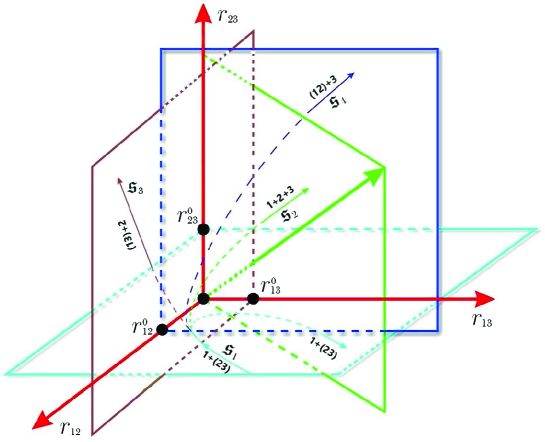
Figure 3: The set of smooth curves ${\mathfrak{s}}=({\mathfrak{s}}_{1},...,{\mathfrak{s}}_{4})$ connecting $(in)$ asymptotic subspace, where the three-body system is in a state $1+(23)$, with $(out)$ asymptotic subspaces, where the following configurations of bodies are formed; $1+(23)$,  $2+(13)$,  $3+(12)$ and $1+2+3$, respectively. The $r_{ij}(\{\bar{\rho}\})\,(i,j=\overline{1,3},\,i\neq{j})$ denotes distance between $i$ and $j$ bodies, and $r^{0}_{ij}$ - the average distance between bodies in the corresponding pair. Note that all the curves $\overline{\mathfrak{s}_{1},\mathfrak{s}_{4}}$ in the subspace $(in)$ merges, which in the figure is shown by continuous blue.

Depending on which particular elementary process is being implemented, the corresponding internal time $s_{i}$ is localized around one of the four smooth curves $\mathfrak{s}_{i}\simeq\mathbb{R}^{1}(i=\overline{1,4}\,)$ connecting two asymptotic scattering subspaces (see FIG. 3).

When scattering between bodies occurs through the formation of a metastable transition complex of bodies $(123)^{\ast}$, the internal time $s_{i}$ can be represented in the form of complex graph $\mathbb{G}=(\mathbb{T},\mathbb{L})$, where $\mathbb{T}=\{\hat{s}_{0},\hat{s}_{1},...,\hat{s}_{n}\}$ denotes a set of tops (turning points of a trajectory $s_{i}$) of graph and $\mathbb{L}$ is a set of ribs of graph $\{\underline{\hat{s}_{0}\hat{s}_{1}},\underline{\hat{s}_{1}\hat{s}_{2}},...,\underline{\hat{s}_{n-1}\hat{s}_{n}}\}$. Recall that, the position of each node in the internal space $\mathbb{E}^{3}$ is determined by three coordinates $\hat{s}_{i}=\hat{s}_{i}(\rho_{1},\rho_{2},\rho_{3})$. Obviously, if to project the graph $\mathbb{G}_{i}$ of corresponding elementary process onto the curve $\mathfrak{s}_{i}$, then the sequence of nodes will be violated, for example, as $\mathfrak{s}_{i}\ni(\breve{\mathfrak{s}}_{0},...\breve{\mathfrak{s}}_{9},\breve{\mathfrak{s}}_{1},...\breve{\mathfrak{s}}_{7},...\breve{\mathfrak{s}}_{8},...\breve{\mathfrak{s}}_{2},...\breve{\mathfrak{s}}_{5},...\breve{\mathfrak{s}}_{4},...)$, where the point $\breve{\mathfrak{s}}_{i}$ denotes the projection of the turning point (node) $\hat{s}_{i}$ on the curve $\mathfrak{s}_{i}.$ It is important to note that, depending on the initial conditions of the problem, internal time $s_{i}$ very often may not have a unequivocal graph representation; moreover, these graphs can be random.

Now, regarding the behavior of a dynamical system depending on the internal time $``s"$. Formally, if in the system of equations (26) we make the replacement $s\to-s$, then it will not change. However, this does not mean at all that the system of equations is invariant with respect to this transformation and, accordingly, is invertible with respect to the timing parameter $``s"$. The fact is that internal time $``s"$ in its structure and sense is very different from ordinary time $t$, the arrow of which is directed forward all the time, connecting the events of the past with the future through the present. In particular, it follows from the above that the points internal time, generally speaking, are not equivalent. This is due to the fact that not only the distances from the origin, but also on which branches of the internal time they are located are important for their determination. Recall that the internal time of a dynamical system $``s"$, after leaving a region where all bodies interact strongly with each other, is divided into four different branches $s=(\overline{s_{1},s_{4}})$, each of which characterizes a specific elementary process. It should be noted that the choice between the marked branches of further evolution of system occurs randomly, for well-known reasons (see the system of equations (38)). In other words, with respect to the transformation $s\to-s$, the system of equations (26) in the general case cannot be invariant.

Finally, to answer the question, the system of equations (26) with respect to the parameter $``s"$ is reversible or not, we will analyze the evolution of the dynamical system from the point of view of the Poincaré’s recurrence theorem Poinc1 ; Poinc2 ; Car1 ; Car2 . To do this, we consider two possible cases $g(\{x\})>0$ and $g(\{x\})\leq 0$.

The case a. (see sec IV) $g(\{x\})>0$ or is equivalently to $\breve{g}(\{\rho\})>0$ (see sec IV), as known corresponds to the three-body scattering problem for which the configuration space $\mathbb{E}^{3}$ is unrestricted, i.e. infinite. Note that for this case, Poincaré’s recurrence theorem is clearly not applicable.

When $g(\{x\})\leq 0$ (or $\breve{g}(\{\rho\})\leq 0$), as mentioned above, we are dealing with a restricted three-body problem. In this case, it it would be natural to expect that the Poincaré’s theorem should be satisfied. Namely, the system should have returned to a state arbitrarily close to its initial state (for systems with a continuous state), after a sufficiently long but finite time. However, even in this case, the Poincaré theorem cannot be is satisfied if we assume the possibility of the existence of various metastable states characterized by distinct groupings of bodies (see Sch.1). In this case, we can only say with some probability that the dynamical system will return close to the initial state for a long, but finite time.

Thus, analyzing the above arguments, it can be stated that irreversibility lies in the very nature of internal time $s=(\overline{s_{1},s_{4}})$, and therefore the system of equations (26) with respect to the timing parameter $``s"$, generally speaking, is irreversible.

VI The restricted three-body problem with holonomic connections

An important class of solutions of the classical three-body problem describes the bound state of three bodies $(123)$, when the motion of bodies occurs in a restricted space. In particular, for gravitating bodies, an exact solutions from this class were founded by a number of outstanding researchers of the 19th and 20th centuries, such as Euler Eul1 ; Eul2 ; Eul3 , Lagrange Lag , Hill Hill ; H1 ; H2 . In the mid-1970s, the new Brooke-Heno-Hadjidemetriu family of orbits was discovered BrB ; HC ; Hen , and in 1993 Moore showed the existence of stable orbits, eights, in which three bodies always catch up with each other. In 2013, by numerical search, 13 new particular solutions were found for the three-body problem, in which the movement of a system of three bodies of the same mass occurs in a repeating cycle Suv . Finally, in 2018, more than 1800 new solutions to the restricted three-body problem were calculated on a supercomputer Xi .

As we will see below, the developed representation has new features and symmetries, which allows us to obtain important information about the restricted three-body problem by analyzing systems of algebraic equations.

Note that the state which will be spatially restricted regardless of the length of time the interaction of bodies cannot be formed as a result of scattering (see Sch. 1) due to the lack of a mechanism for removing energy from the system. Nevertheless, it is clear that the character of the motions of bodies in the states $(123)$ and $(123)^{\star}$ in many of features should be similar. In any case, the solutions of the system (27) must satisfy the energy conservation law (30) that defines $5D$ hypersurface in the $6D$ phase space.

Some important properties of this problem can be studied by algebraic methods without solving the equations of motion (26) or (27). In particular, it is very interesting to find solutions for which the connections between bodies remain holonomic throughout the movement. Recall that this situation is especially interesting for three gravitating bodies.

Proposition 3. The three-body system can forms a stable configuration with holonomic connections, if in the equations system (27) all projections of geodetic acceleration are equal to zero $\ddot{x}^{i}=0\,\,(i=\overline{1,3}\,)$, and if there is non-empty continuous set $\mathbb{E}^{3}\supset\Xi\neq\oslash$, on which the determinant of the obtained algebraic system is equal to zero.

Proof.

Let consider the case when the center of mass (imaginary point) of a system of bodies moves along the manifold $\mathcal{M}^{(3)}_{\{\bar{J}\}}$ without acceleration, i.e. $\ddot{x}^{i}=0\,\,(i=\overline{1,3}\,)$. This means, we can simplify the system of equations (27) by writing their in the form:

$$a_{1}\bigl{\{}(\xi^{1})^{2}-(\xi^{2})^{2}-(\xi^{3})^{2}-\Lambda^{2}\bigr{\}}+2\xi^{1}\bigl{\{}a_{2}\xi^{2}+a_{3}\xi^{3}\bigr{\}}=0,$$

$$a_{2}\bigl{\{}(\xi^{2})^{2}-(\xi^{3})^{2}-(\xi^{1})^{2}-\Lambda^{2}\bigr{\}}+2\xi^{2}\bigl{\{}a_{3}\xi^{3}+a_{1}\xi^{1}\bigr{\}}=0,$$

$$a_{3}\bigl{\{}(\xi^{3})^{2}-(\xi^{1})^{2}-(\xi^{2})^{2}-\Lambda^{2}\bigr{\}}+2\xi^{3}\bigl{\{}a_{1}\xi^{1}+a_{2}\xi^{2}\bigr{\}}=0.$$ (48)

From the conditions of the absence of acceleration it follows that the projections of the geodetic velocity $\xi^{1},\,\xi^{2}$ and $\xi^{3}$ are constants and, accordingly, equations (48) can be solved with respect to three unknown coefficients:

$$a_{i}(\{\bar{x}\})=\Delta_{i}(\{\bar{x}\})\Delta^{-1}(\{\bar{x}\}),\qquad i=\overline{1,3},$$ (49)

where the determinant $\Delta(\{\bar{x}\})$ has the form:

$$\Delta(\{\bar{x}\})=\left|\begin{array}[]{ccc}K_{1}&2\xi^{1}\xi^{2}&2\xi^{1}\xi^{3}\\ 2\xi^{1}\xi^{2}&K_{2}&2\xi^{2}\xi^{3}\\ 2\xi^{1}\xi^{3}&2\xi^{2}\xi^{3}&K_{3}\end{array}\right|,\qquad\begin{array}[]{ccc}K_{1}(\{\bar{x}\})=(\xi^{1})^{2}-(\xi^{2})^{2}-(\xi^{3})^{2}-\Lambda^{2}(\{\bar{x}\}),\\ K_{2}(\{\bar{x}\})=(\xi^{2})^{2}-(\xi^{3})^{2}-(\xi^{1})^{2}-\Lambda^{2}(\{\bar{x}\}),\\ K_{3}(\{\bar{x}\})=(\xi^{3})^{2}-(\xi^{1})^{2}-(\xi^{2})^{2}-\Lambda^{2}(\{\bar{x}\}).\end{array}$$ (56)

As for the determinant $\Delta_{i}(\{\bar{x}\})$, they can be found from the third-order determinant (56), replacing the elements of the $i$-th column with zeros. In other words; $\Delta_{1}(\{\bar{x}\})=\Delta_{2}(\{\bar{x}\})=\Delta_{3}(\{\bar{x}\})=0$, and, respectively, the system of equations (48) will have a non-trivial solution if the determinant of the system (48) is equal to zero too, i.e. $\Delta(\{\bar{x}\})=0$. More precisely, the system of equations (48) will have solutions if in expressions (49), uncertainties of the type $0/0$ can be eliminated. As the study shows, there always exists a non-empty continuous set $\Xi\neq\oslash$, on which the determinant of algebraic equations (48) is equal to zero and, accordingly, the above uncertainty is eliminated (see Appendix E for details).

Proposition 3 is proved.

VII Deviation of geodesic trajectories of one family

Studying the linear deviations of the geodesic trajectories of one family, one can get valuable information about the properties of a dynamical system and, very importantly, about the relationship between the behavior of a dynamical system and the geometric features of a Riemannian space.

Definition 6. Let $x^{i}=x^{i}(s,\eta)$ be the equation of a one-parameter family of geodesics on the Riemannian manifold $\mathcal{M}^{(3)}_{\bar{J}}$, where $s$ is an affine parameter along geodesic the trajectory, whereas the symbol $\eta$ denotes the family parameter. The vector $\mathbf{j}(\{\zeta\})$ in the direction of the normal of the geodesic $\mathbf{l}(\{\bar{x}\})$ with components:

$$\frac{\delta x^{i}(s,\eta)}{\delta\eta}=\zeta^{i}(s,\eta),\qquad\{\zeta\}=(\zeta^{1},\zeta^{2},\zeta^{3}),\quad i=\overline{1,3},$$ (57)

will be called the linear deviation of close geodesics.

The components of the deviation vector $\mathbf{j}(\{\zeta\})$ satisfy the following equations BubrNovFom :

$$\frac{\mathcal{D}^{2}\zeta^{i}}{\mathcal{D}s^{2}}=-\mathcal{R}^{i}_{jkl}(\{\bar{x}\})x^{j}\zeta^{k}x^{l},\qquad i,j,k,l=\overline{1,3},$$ (58)

where $\mathcal{R}^{i}_{jkl}(\{\bar{x}\})$ is the Riemann tensor, which has the form:

$$\mathcal{R}^{i}_{jkl}=\Gamma^{i}_{lj,\,k}-\Gamma^{i}_{jk,\,l}+\Gamma^{i}_{k\lambda}\Gamma^{\lambda}_{lj}-\Gamma^{i}_{l\lambda}\Gamma^{\lambda}_{jk},\qquad\Gamma^{i}_{jk,\,l}(\{\bar{x}\})=\partial\Gamma^{i}_{jk}(\{\bar{x}\})/\partial x^{l}.$$ (59)

The equation (58) can be written in the form of an ordinary second-order differential equation:

$$\ddot{\zeta}^{i}+2\Gamma^{i}_{j\,l}\dot{x}^{j}\dot{\zeta}^{l}+\bigl{(}\dot{\Gamma}^{i}_{j\,l}\dot{x}^{j}-\Gamma^{i}_{j\,l}\Gamma^{j}_{k\,p}\dot{x}^{k}\dot{x}^{p}+\Gamma^{i}_{j\,n}\Gamma^{n}_{k\,p}\,\dot{x}^{j}\dot{x}^{k}\delta_{l}^{p}\bigr{)}\zeta^{l}=-\mathcal{R}^{i}_{jkl}\,x^{j}\zeta^{k}x^{l},$$ (60)

The explicit form of specific terms of the equation (60) can be found in the appendix F. Solving equation (60) together with the equations systems (26) and (38), we can get a full view on deviation properties of close geodesic trajectories of a one-parameter family, which is a very important characteristic of a dynamical system.

VIII Three-body system in a random environment

Let us suppose that a three-body system is subject to external influences that have regular and random components. The causes of such impacts can be different. For example, when a system of bodies is immersed in the environment - gas, liquid, etc. In this case, the total energy of the system of bodies changes due to random collisions. Given the new conditions, the three-body problem can be mathematically generalized if to assume that in the system of equations (27) the metric tensor $g_{ij}(\{\bar{x}\})$ is random.

When studying atomic-molecular processes even in a vacuum, it is often important to take into account the influence of quantum fluctuations on the classical dynamics of interacting bodies.

In the simplest case, when an external random force acts on the dynamical system without deformation of the metric tensor $g_{ij}(\{\bar{x}\})$, using the system of equations (27), we can write the following system of stochastic differential equations (SDE) to describe the motion of three bodies:

$$\dot{\chi}^{\mu}=A^{\mu}(\{\chi\})+\eta^{\mu}(s),\qquad\mu=\overline{1,6},$$ (61)

where the independent variables $\{\chi\}=\bigl{(}\{\bar{x}\},\{\bar{\xi}\}\bigr{)}=\overline{\chi^{1},\chi^{6}}$ form the Euclidean $6D$ space, in addition, the following notations are made:

$$\chi^{1}={\xi}^{1},\qquad\chi^{2}={\xi}^{2},\qquad\chi^{3}={\xi}^{3},\qquad\chi^{4}=x^{1},\qquad\chi^{5}={x}^{2},\qquad\chi^{6}={x}^{3}.$$

In addition, in (61), the coefficients $A^{\mu}(\{\chi\})$ are defined by the expressions:

$$A^{1}\bigl{(}\{\chi\}\bigr{)}=a_{1}\bigl{\{}(\xi^{1})^{2}-(\xi^{2})^{2}-(\xi^{3})^{2}-\Lambda^{2}\bigr{\}}+2\xi^{1}(a_{2}\xi^{2}+a_{3}\xi^{3}),\qquad A^{4}\bigl{(}\{\chi\}\bigr{)}=\xi^{1},$$

$$A^{2}\bigl{(}\{\chi\}\bigr{)}=a_{2}\bigl{\{}(\xi^{2})^{2}-(\xi^{1})^{2}-(\xi^{3})^{2}-\Lambda^{2}\bigr{\}}+2\xi^{2}(a_{3}\xi^{3}+a_{1}\xi^{1}),\qquad A^{5}\bigl{(}\{\chi\}\bigr{)}=\xi^{2},$$

$$A^{3}\bigl{(}\{\chi\}\bigr{)}=a_{3}\bigl{\{}(\xi^{3})^{2}-(\xi^{2})^{2}-(\xi^{1})^{2}-\Lambda^{2}\bigr{\}}+2\xi^{3}(a_{1}\xi^{1}+a_{2}\xi^{2}),\qquad A^{6}\bigl{(}\{\chi\}\bigr{)}=\xi^{3}.$$

Recall that $A^{\mu}(\{\chi\})$ are regular functions.

For simplicity, we assume that the stochastic functions $\eta^{\mu}(s)$ satisfy the correlation relations of white noise:

$$\langle\eta^{\mu}(s)\rangle=0,\qquad\langle\eta^{\mu}(s)\eta^{\mu}(s^{\prime})\rangle=2\epsilon\delta(s-s^{\prime}),$$ (62)

where $\epsilon$ denotes the power of random fluctuations and $\delta(s-s^{\prime})$ is the Dirac delta function.

Now we can move on to the problem of deriving the equation of joint probability density (JPD) for the independent variables $\{\chi\}$.

For further analytical study of the problem, it is convenient to present JPD in the form:

$$P\bigl{(}\{\chi\},s\bigr{)}=\prod_{\mu=1}^{6}\bigl{\langle}\delta\bigl{[}\chi^{\mu}(s)-\chi^{\mu}\bigr{]}\bigr{\rangle}.$$ (63)

Using a well-known technique (see Kljat ; Lif ), we can differentiate the expression (63) by internal time $``s"$ and taking into account (61) and (62) get the following second-order partial differential equation (PDF):

$$\frac{\partial P}{\partial s}=\sum_{\mu=1}^{6}\frac{\partial}{\partial\chi^{\mu}}\Bigl{[}A^{\mu}\bigl{(}\{\chi\}\bigr{)}+\epsilon\frac{\partial}{\partial\chi^{\mu}}\Bigr{]}P.$$ (64)

It is easy to see the function (64) determines the probability of the position and momentum of imaginary point characterizing the three-body system in the $6D$ phase space. In the case when $\epsilon=\hbar$, the function $P\bigl{(}\{\chi\},s\bigr{)}$ in principle play the same role as the Wigner quasi-probability distribution Wig ; Weil . However, unlike the Wigner function, which in some regions of the phase space can take negative values, and therefore is not a probability distribution, the solution of the equation (64) is positive definite in the entire phase space. In other words, the function $P\bigl{(}\{\chi\},s\bigr{)}$ really has the meaning of a probability distribution, which describes the probabilistic evolution of the classical three-body system in phase space taking into account the influence of quantum fluctuations.

Developing the same ideology, we can obtain the equation of probability distribution of an elementary process in momentum and coordinate representations, taking into account the influence of the environment.

In particular, for the probability current in the momentum representation $P^{(m)}_{\{\bar{x}\}}\bigl{(}\{\bar{\xi}\}\bigr{)}$, at the point $\{\bar{x}\}\ni\mathbb{E}^{3}$ we obtain the following second-order PDF:

$$\dot{P}^{(m)}_{\{\bar{x}\}}=\sum_{i=1}^{3}\frac{\partial}{\partial\xi^{i}}\Bigl{[}A^{i}\bigl{(}\{\bar{x}\},\{\bar{\xi}\}\bigr{)}+\epsilon\frac{\partial}{\partial\xi^{i}}\Bigr{]}P^{(m)}_{\{\bar{x}\}},\qquad\dot{P}^{(m)}_{\{\bar{x}\}}=\partial{P}^{(m)}_{\{\bar{x}\}}/\partial{s}.$$ (65)

In other words, by calculating equation (65) at a given point $\{\bar{x}\}$, we can find the distribution of the velocity (momentum) $\{\bar{\xi}\}$ of the imaginary point depending on the internal time $``s"$. We can also trace the evolution of the momentum distribution along the trajectory by substituting $\{\bar{x}\}\to\{\bar{x}(s)\}$ in the equation (65). Note that in this case the equation (65) is solved in combination with the system of equations (27).

Now we consider the case when the metric of the internal space $\mathbb{E}^{3}$ depending on the internal time $``s"$ is continuous, however its first derivative is already a random function. The above task will be mathematically equivalent to random mappings of the type:

$$R_{f}:a_{i}\bigl{(}\{\bar{x}\}\bigr{)}\mapsto\tilde{a}_{i}\bigl{(}s,\{\bar{x}\}\bigr{)}=\frac{d}{dx^{i}}\ln g\bigl{(}s,\{\bar{x}\}\bigr{)},\qquad i=\overline{1,3},$$

or more detail:

$$\tilde{a}_{i}\bigl{(}s,\{\bar{x}\}\bigr{)}=\frac{\partial\ln\tilde{g}\bigl{(}s,\{\bar{x}\}\bigr{)}}{\partial x^{i}}+\frac{\partial s}{\partial x^{i}}\frac{\partial\ln\tilde{g}\bigl{(}s,\{\bar{x}\}\bigr{)}}{\partial s}=\tilde{a}_{i}(s,\{\bar{x}\}\bigr{)}+\frac{\dot{\tilde{g}}(s,\{\bar{x}\}\bigr{)}}{\sqrt{\tilde{g}(s,\{\bar{x}\}\bigr{)}}},$$ (66)

where $\tilde{a}_{i}\bigl{(}s,\{\bar{x}\}\bigr{)}$ are regular functions, $R_{f}$ denotes the operator of random mappings and $\tilde{\eta}\bigl{(}s,\{\bar{x}\}\bigr{)}=\dot{\tilde{g}}/\sqrt{\tilde{g}}$ is a random function, which will be defined below. Taking into account the above, the system of equations (27) can be decomposed and presented in the form of stochastic Langevin type equations:

$$\dot{\xi}^{\mu}=A^{\mu}\bigl{(}\{\chi\}\bigr{)}+B^{\mu}\bigl{(}\{\chi\}\bigr{)}\eta\bigl{(}s,\{\bar{x}\}\bigr{)},\qquad\mu=\overline{1,6},$$ (67)

where

$$B^{1}\bigl{(}\{\chi\}\bigr{)}=\bigl{(}\xi^{1}\bigr{)}^{2}-\bigl{(}\xi^{2}\bigr{)}^{2}-\bigl{(}\xi^{3}\bigr{)}^{2}+2\xi^{1}\bigl{(}\xi^{2}+\xi^{3}\bigr{)}-{\Lambda}^{2}(\{\bar{x}\}),\qquad B^{4}\bigl{(}\{\chi\}\bigr{)}=0,$$

$$B^{2}\bigl{(}\{\chi\}\bigr{)}=\bigl{(}\xi^{2}\bigr{)}^{2}-\bigl{(}\xi^{1}\bigr{)}^{2}-\bigl{(}\xi^{3}\bigr{)}^{2}+2\xi^{2}\bigl{(}\xi^{1}+\xi^{3}\bigr{)}-{\Lambda}^{2}(\{\bar{x}\}),\qquad B^{5}\bigl{(}\{\chi\}\bigr{)}=0,$$

$$B^{3}\bigl{(}\{\chi\}\bigr{)}=\bigl{(}\xi^{3}\bigr{)}^{2}-\bigl{(}\xi^{2}\bigr{)}^{2}-\bigl{(}\xi^{1}\bigr{)}^{2}+2\xi^{3}\bigl{(}\xi^{1}+\xi^{2}\bigr{)}-{\Lambda}^{2}(\{\bar{x}\}),\qquad B^{6}\bigl{(}\{\chi\}\bigr{)}=0.$$

The JPD for the independent variables $\{\chi\}$ again can be represented in the form (63). For simplicity we will assume that a random generator $\tilde{\eta}\bigl{(}s,\{\bar{x}\}\bigr{)}=\eta\bigl{(}s\bigr{)}/\sqrt{g}$ and, in addition, that it satisfy the correlation properties of the white noise with fluctuation power $\epsilon$ (see (62)). Further, performing calculations similar to (63)-(64) using the SDE (67), we get the following second-order PDE for JPD:

$$\frac{\partial P}{\partial s}=\sum_{\mu=1}^{6}\frac{\partial}{\partial\xi^{\mu}}\bigl{(}A^{\mu}P\bigr{)}+\epsilon g^{-1/2}\sum_{i,j=1}^{3}\frac{\partial}{\partial\xi^{i}}\Bigl{[}B^{i}\frac{\partial}{\partial\xi^{j}}\bigl{(}B^{j}P\bigr{)}\Bigr{]}.$$ (68)

Finally, for the probabilistic current in the momentum representation at the given point $\{\bar{x}\}\in\mathbb{E}^{3}$ we get the following second-order PDF:

$$\dot{P}^{(m)}_{\{\bar{x}\}}=\sum_{i=1}^{3}\frac{\partial}{\partial\xi^{i}}\bigl{(}A^{i}P\bigr{)}+\epsilon g^{-1/2}\sum_{i,j=1}^{3}\frac{\partial}{\partial\xi^{i}}\Bigl{[}B^{i}\frac{\partial}{\partial\xi^{j}}\bigl{(}B^{j}{P}^{(m)}_{\{\bar{x}\}}\bigr{)}\Bigr{]}.$$ (69)

Substituting $\{\bar{x}\}\to\{\bar{x}(s)\}$ into the equation (69), we can study the evolution of the momentum distribution along the trajectory of a dynamical system.

Thus, we have obtained equations describing geodesic flows in the phase space (64) and (68), as well as in the momentum space (65) and (69), which must be solved in combination with a system of differential equations of the first order (27). Recall that the method used to obtain the noted equations can be attributed to Nelson’s type stochastic quantization Nelson , with the only difference being that internal time $``s"$ cardinally changes the sense of the developed approach. In particular, in the limit $\epsilon\to 0$, the representation allows a continuous transition from the statistical (see (64) and (68)) to the dynamical description (see (27)) of the problem.

IX A new criterion for estimating chaos in classical systems

When the three-body system is in an environment that has both regular and random influences on it, then it makes sense to talk about a statistical system. In this case, the main task is to construct the mathematical expectations of different elementary atomic-molecular processes occurring during multichannel scattering (see Sch. 1). Recall that the evolution equations (64) and (68), describing of geodesic flows depending on internal time $``s"$ have an important feature. The latter circumstance makes it necessary to introduce new criteria for determining the measure of deviation of probabilistic current tubes of various elementary processes.

In particular, following the definition of Kullback-Leibler definition of the distance between two continuous distributions, we can determine the criterion characterizing the deviation between the corresponding tubes of probabilistic currents Kul .

Definition 7. The deviation between two different tubes of probabilistic currents in the phase space will be defined by the expression:

$$d(s_{a},s_{b})=\int_{\mathcal{P}^{6}}P\bigl{(}\{\chi\},s_{a}\bigr{)}\ln\biggl{|}\frac{P\bigl{(}\{\chi\},s_{a}\bigr{)}}{P\bigl{(}\{\chi\},s_{b}\bigr{)}}\biggr{|}\sqrt{g(\{\bar{x}\})}\prod_{\nu=1}^{6}d\chi^{\nu},$$ (70)

where $P_{a}\equiv P\bigl{(}\{\chi\},s_{a}\bigr{)}$ and $P_{b}\equiv P\bigl{(}\{\chi\},s_{b}\bigr{)}$ are two different probabilistic currents, which at the beginning of development of elementary processes are closely located or have an intersection.

In the case when the distance between two flows depending on internal times $s\sim s_{a}\sim s_{b}$ grows linearly, that is:

$$d(s)\sim ks,\qquad k=const>0,$$

there is reason to believe that a dynamical system exhibits chaotic behavior, i.e. it is chaotic.

Definition 8. Let $P_{if}(s_{n})$ be the transition probability between the $(in)$ and $(out)$ asymptotic channels with the internal time $s_{n}$, then the total mathematical expectation of the transition between two asymptotic states $P_{ab}^{tot}$ will be defined as:

$$P_{if}^{tot}=\lim_{N\to\infty}\biggl{[}\frac{1}{N}\sum_{n=1}^{N}\Bigl{(}\lim_{s_{n}\to\,\infty}P_{if}(s_{n})\Bigr{)}\biggr{]},$$ (71)

where $N$ denotes the number of various solutions of the Cauchy problem for the system (27).

X The quantum three-body problem on conformal-Euclidean manifold

If the classical three-body problem plays a fundamental role for understanding the dynamics of complex classical systems, then a similar problem in quantum mechanics is the key to studying the atomic and subatomic nature of matter. In this regard, it is obvious that a mathematically rigorous description of the system of interacting atoms is a task of primary importance. Note that the first work on this problem was carried out by Skorniakov and Ter-Martirosian Ter . Recall that they derived equations for determining the wave function of a system of three identical particles in the limiting case of zero-range forces. The approach was generalized by Faddeev for arbitrary particles and the finite-range forces Faddeev . Scattering in three-particle atomic-molecular systems is characterized by both two-particle and three-particle interactions, which makes the Faddeev approach inaccurate for describing such processes. In this regard, subsequently, various approaches and corresponding algorithms were developed for studying atomic-molecular processes in the framework of the three-body scattering problem (see for example Kosloff ; Balint-Kurti ). However, on the way to the description of quantum multichannel scattering, in our opinion, a new fundamental ideological problem arose related to the paper of Hanney and Berry Hannay (see also Schuster ). Namely, as the authors proved in this paper, in the limit $\hbar\to 0$ there is no transition from the $Q$ system (quantum systems) to the $P$-system (Poincaré systems) (see FIG. 4 ).

To solve the open problem of quantum-classical correspondence, the three-body problem is an ideal model, since this system very often exhibits strongly developed chaotic behavior in the classical limit. Recall that by strongly developed chaos we imply a such state of the classical system, when the chaotic region in the $2n$ -dimensional phase space occupies a larger volume than the volume of the quantum cell - ${\hbar}^{n}$. Obviously, in this case the so-called quantum suppression of chaos does not occur, and we must observe chaos in the behavior of the wave function itself.

Using the reduced classical Hamiltonian (28), we can write the following non-stationary quantum for the three-body system in conformal-Euclidean space (internal space) $\mathcal{M}^{(3)}$:

$$i\hbar\frac{\partial\Psi}{\partial s}=\hat{\mathcal{H}}\bigl{(}\{\bar{x}\};\{\bar{p}\}\bigr{)}\Psi,$$ (72)

where $\hat{\mathcal{H}}$ is the Hamiltonian of the quantum problem.

By making the following substitutions in the reduced classical Hamiltonian (28):

$$\dot{x}^{i}\to-i\hbar\partial/\partial x^{i}\quad and\quad J^{2}\to J(J+1),$$

which is equivalent to the transition to the quantum Hamiltonian (see Zom ), we get:

$$\hat{\mathcal{H}}\bigl{(}\{\bar{x}\};\{\bar{p}\}\bigr{)}=\frac{1}{2\mu_{0}}\biggl{\{}-\hbar^{2}g(\{\bar{x}\})\sum_{i=1}^{3}\frac{\partial^{2}}{(\partial x^{i})^{2}}+\frac{J(J+1)}{g(\{\bar{x}\})}\biggr{\}}.$$ (73)

In the case when the energy of the three-body system is fixed, that is, $\mathrm{E}=const$, we can go to the stationary equation for the wave function.

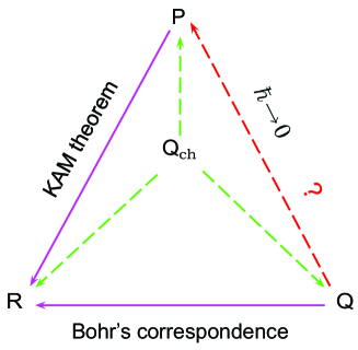
Figure 4: The figure shows a diagram of the interconnections between the three well-known regions of matter motion ${\mathbf{R}},{\mathbf{P}},{\mathbf{Q}}$ and the new region ${\mathbf{Q}}_{ch}$, which is strictly defined in this paper. Recall that ${\mathbf{R}}$ denotes classical regular systems (Newton systems), ${\mathbf{P}}$ denotes classical dynamically or chaotic systems (Poincaré systems), ${\mathbf{Q}}$ denotes regular quantum systems and ${\mathbf{Q}}_{ch}$ - quantum chaotic systems. There is a possibility of passing from the ${\mathbf{P}}$ system to the ${\mathbf{R}}$ system, which is ensured by the KAM-theorem Poschel . From the system ${\mathbf{Q}}$, a transition to the system ${\mathbf{R}}$ is possible, but not to the system ${\mathbf{P}}$, while from the system ${\mathbf{Q}}_{ch}$ there is the possibility of transition to all three ${\mathbf{R}},{\mathbf{P}}$ and ${\mathbf{Q}}$ systems.

In particular, substituting the wave function:

$$\Psi\bigl{(}\{\bar{x}\},s\bigr{)}=\exp\bigl{(}-i\mathrm{E}s/{\hbar}\bigr{)}\bar{\Psi}\bigl{(}\{\bar{x}\}\bigr{)},$$

into the equation (72) - (73), we obtain the following stationary equation:

$$\Biggl{\{}\sum_{i=1}^{3}\frac{\partial^{2}}{(\partial x^{i})^{2}}+\frac{2\mu_{0}}{\hbar^{2}g(\{\bar{x}\})}\biggl{[}\mathrm{E}-\frac{J(J+1)}{g(\{\bar{x}\})}\biggr{]}\Biggr{\}}\bar{\Psi}(\{\bar{x}\})=0.$$ (74)

Recall that $J^{2}=\sum_{i=1}^{3}J^{2}_{i}=const$ is the total angular momentum of the system of bodies, which in this case is quantized.

For any fixed $\bf J$, there is a countable number of submanifolds:

$$\mathcal{M}^{(3)}_{\{\bf J\}}=\bigl{\{}\mathcal{M}^{(3)}_{\{\alpha\}}\bigr{\}}_{\alpha\in\mathcal{B}_{\bf J}},$$

on which various quantum processes flow, where $\mathcal{B}_{\bf J}$ is the family of sets with different projections of $J_{z}$. Recall that these submanifolds differ by its orientations in the $6D$ manifold (space) $\mathcal{M}$, which we can determine with two commutated quantum numbers ${\{\bf J\}}=(J,J_{z})$. In other words, in the developed approach when quantizing a dynamical problem, a typical example of which is the three-body problem, geometry is also quantized.

In particular, when ${\bf J}=0$ there is only one submanifold $\mathcal{M}^{(3)}_{\{\bf{0}\}}$, where ${\{\bf{0}\}}=(0,0)$. In the case when ${\bf J}=\bf 1$, there exists a family of three oriented submanifolds, on each of which the Schrödinger equation is invariant:

$$\mathcal{M}^{(3)}_{\{\bf{1}\}}=\bigl{\{}\mathcal{M}^{(3)}_{\{\alpha\}}\bigr{\}}_{\alpha\in\mathcal{B}_{\bf 1}},\qquad\mathcal{B}_{\bf 1}=\bigl{\{}(1,+1),\,(1,0),\,(1,-1)\bigr{\}},$$

We can combine submanifolds of a family with a given full rotational momentum $\bf J$, as is done in the case of a family of sets:

$$\mathcal{M}^{(3)}_{\bm{1}}=\bigcup_{\alpha\in\mathcal{B}_{\bm{1}}}\mathcal{M}^{(3)}_{\{\alpha\}}=\bigl{\{}\{\bar{x}\}|\,\exists\,\alpha\in\mathcal{B}_{\bm{1}},\,\{\bar{x}\}\in\mathcal{M}^{(3)}_{\alpha}\bigr{\}}.$$

For further analytical constructions of the problem, it is useful to introduce a new coordinate systems on the cards $G_{\alpha}$, arising at continuously mappings $f:\{\bar{\rho}\}\mapsto\{\bar{x}\}$.
We will consider two important cases:

a. When three bodies form a bound state, i.e. $g(\{\bar{x}\})\leq 0$, and, accordingly,

b. when scattering in a system occurs with a rearrangement of bodies, for example; $1+(23)\to(12)+3$ (see Sch. 1). Recall that in this case the scattering processes in the system occur under the condition $g(\{\bar{x}\})>0.$

X.1 The three-body coupled states

First, consider the case a., when three bodies form a bound state. For this case, it is convenient to use a local spherical coordinate system (LSCS) (see FIG. 5):

$$\{\bar{\mathrm{r}}\}=\bigl{(}\mathrm{r},\theta,\varphi\bigr{)},\qquad\mathrm{r}^{2}=\bigl{(}x^{1}\bigr{)}^{2}+\bigl{(}x^{2}\bigr{)}^{2}+\bigl{(}x^{3}\bigr{)}^{2},\qquad\theta\in\bigl{[}0,\pi\bigr{]},\qquad\varphi\in\bigl{[}0,2\pi\bigr{]}.$$

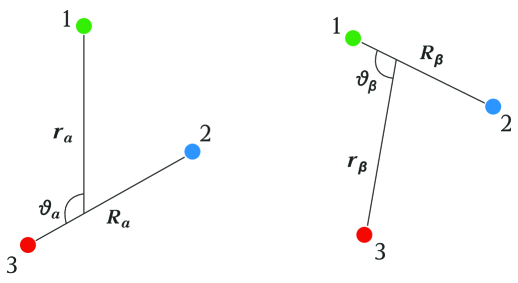
Figure 6: The set of Jacobi coordinates $(\textbf{R}_{\alpha},\textbf{r}_{\alpha},\vartheta_{\alpha})$ is convenient for describing the asymptotic states $1+(23)_{njK}$, whereas another set of Jacobi coordinates $(\textbf{R}_{\beta},\textbf{r}_{\beta},\vartheta_{\beta})$ is convenient for describing the asymptotic states $(12)_{n^{\prime}j^{\prime}K^{\prime}}+3.$

Note that this is firstly due to the fact that, in a geometric sense, bound states are localized on 2$D$ closed surfaces that are homeomorphic with isolated spheres having topological features (Appendix D, family ${\breve{\mathcal{A}}}$ see FIG. 6 ).

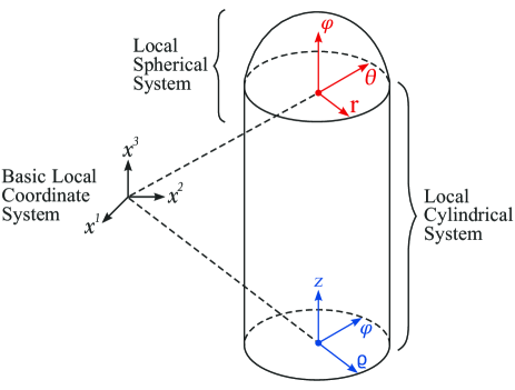
Figure 5: When constructing the representation on the atlas card, a rectangular local coordinate system (we call the basic local coordinate system) $\{\bar{x}\}=(x^{1},x^{2},x^{3})$ is determined. However, for further studies of the quantum problem it is useful to use the local spherical coordinate system $\{\bar{\mathrm{r}}\}=(\mathrm{r},\theta,\varphi)$ to describe the bound quantum state, and the local cylindrical coordinate system $\{\bar{\mathrm{\varrho}}\}=(\mathrm{\varrho},z,\varphi)$, respectively, to describe multichannel quantum scattering.

Within the framework of LSCS, the equation (74) can be written as:

$$\Biggl{\{}\Delta+\frac{2\mu_{0}}{\hbar^{2}g_{\varepsilon}\bigl{(}\{\bar{\mathrm{r}}\}\bigr{)}}\biggl{[}\mathrm{E}-\frac{J(J+1)}{g_{\varepsilon}\bigl{(}\{\bar{\mathrm{r}}\}\bigr{)}}\biggr{]}\Biggr{\}}\bar{\Psi}=0.$$ (75)

where $\Delta$ denotes Laplace operator in the LSCS, in addition, $f:g(\{\bar{x}\})\mapsto g_{\varepsilon}(\{\bar{\mathrm{r}}\})$:

$$\Delta=\frac{1}{\mathrm{r}^{2}}\frac{\partial}{\partial\mathrm{r}}\biggl{(}\mathrm{r}^{2}\frac{\partial}{\partial\mathrm{r}}\biggr{)}+\frac{1}{\mathrm{r}^{2}\sin\theta}\frac{\partial}{\partial\theta}\biggl{(}\sin\theta\frac{\partial}{\partial\theta}\biggr{)}+\frac{1}{\mathrm{r}^{2}\sin^{2}\theta}\frac{\partial^{2}}{\partial\varphi^{2}}.$$

Recall that the function $g_{\varepsilon}\bigl{(}\{\bar{\mathrm{r}}\}\bigr{)}$ is obtained from $g(\{\bar{x}\};\varepsilon)=\bigl{[}\mathrm{E}+i\varepsilon-U(\{\bar{x}\})\bigr{]}U^{-1}_{0}\neq 0$, where $\varepsilon\ll 1$ (see (19)), after transition into the LSCS. Note that the small parameter $\varepsilon$ has a physical meaning, namely, it characterizes the width of the energy level of the quantum state. Since the Laplace spherical harmonics $Y_{l}^{m}(\theta,\varphi)$ form an orthonormal basis of the Hilbert space of quadratically integrable functions Arfken , we can use this property and write equation (75) in the form:

$$\Biggl{\{}\Delta+\frac{2\mu_{0}}{\hbar^{2}}\sum_{\bar{l}=0}^{\infty}\sum_{\bar{m}=-\bar{l}}^{\bar{l}}\Omega_{\bar{l}\bar{m}}({\mathrm{r}};\,\mathrm{E},J,\varepsilon)Y_{\bar{l}}^{\bar{m}}(\theta,\varphi)\Biggr{\}}\bar{\Psi}=0,$$ (76)

where

$$\Omega_{\bar{l}\bar{m}}({\mathrm{r}};\,\mathrm{E},J,\varepsilon)=\bigl{[}\mathrm{E}\,\mathfrak{g}^{(1)}_{\bar{l}\bar{m}}(\mathrm{r};\varepsilon)-J(J+1){g}^{(2)}_{\bar{l}\bar{m}}(\mathrm{r};\varepsilon)\bigr{]},$$

$${g^{-k}_{\varepsilon}\bigl{(}\{\bar{\mathrm{r}}\}\bigr{)}}=\sum_{\bar{l}=0}^{\infty}\sum_{\bar{m}=-\bar{l}}^{\bar{l}}\mathfrak{g}^{(k)}_{\bar{l}\bar{m}}(\mathrm{r};\,\varepsilon)\,Y_{\bar{l}}^{\bar{m}}(\theta,\varphi),\qquad k=1,2.$$

It is easy to find the functions $\mathfrak{g}^{(1)}_{\bar{l}\bar{m}}(\mathrm{r};\,\varepsilon)$ and $\mathfrak{g}^{(2)}_{\bar{l}\bar{m}}(\mathrm{r};\,\varepsilon)$. For this we need to multiply the corresponding expressions for the functions $g^{-1}_{\varepsilon}\bigl{(}\{\bar{\mathrm{r}}\}\bigr{)}$ and $g^{-2}_{\varepsilon}\bigl{(}\{\bar{\mathrm{r}}\}\bigr{)}$ on the complex conjugation of a spherical function $Y_{\bar{l}^{\prime}}^{\bar{m}^{\prime}\ast}(\theta,\varphi)$, and then to integrate over the sphere of unit radius:

$$\mathfrak{g}^{(k)}_{\bar{l}\bar{m}}(\mathrm{r};\,\varepsilon)=\int_{0}^{2\pi}\int_{0}^{\pi}g^{-k}_{\varepsilon}\bigl{(}\{\bar{\mathrm{r}}\}\bigr{)}Y_{\bar{l}}^{\bar{m}\ast}(\theta,\varphi)\sin\theta{d\theta d\varphi},\qquad k=1,2.$$

We can consider the problem of finding solutions in the form:

$$\bar{\Psi}\bigl{(}\mathrm{r},\theta,\varphi;\,\varepsilon\bigr{)}=\Upsilon(\mathrm{r};\varepsilon)Y_{l}^{m}(\theta,\varphi).$$ (77)

where $\Upsilon(\mathrm{r};\varepsilon)$ describes a radial wave function.

Substituting (77) into the equation (76) and performing simple calculations, we can find the following ordinary differential equation (ODE) (see Appendix G):

$$\biggl{\{}\frac{1}{{\mathrm{r}}^{2}}\frac{\mathrm{d}}{\mathrm{d}\mathrm{r}}\biggl{(}{\mathrm{r}}^{2}\frac{\mathrm{d}}{\mathrm{d}{{\mathrm{r}}}}\biggr{)}-\frac{l(l+1)}{{\mathrm{r}}^{2}}+\frac{2\mu_{0}}{\hbar^{2}}\sum_{\bar{l}=0}^{2l}\sum_{\bar{m}=\,0}^{\bar{l}}\overline{\mathcal{W}}_{m,\bar{m}\,;\,l,\bar{l}}\,\Omega_{\bar{l}\bar{m}}\bigl{(}{\mathrm{r}};\,\mathrm{E},J,\varepsilon\bigr{)}\biggr{\}}\Upsilon=0,$$ (78)

where $l=0,1,2,...$ is the quantum number of angular momentum in the internal space $\mathcal{M}^{(3)}$, in addition:

$$\overline{\mathcal{W}}_{m,\bar{m};\,l,\bar{l}}=\sqrt{\frac{2\bar{l}+1}{\pi}}\biggl{(}l+\frac{1}{2}\biggr{)}\biggl{(}\begin{array}[]{ccc}l&l&\bar{l}\\ 0&0&0\end{array}\biggr{)}\biggl{(}\begin{array}[]{ccc}l&l&\bar{l}\\ -|m|&-|m|&|\bar{m}|\end{array}\biggr{)}.$$ (83)

Thus, we have obtained a one-dimensional equation for the radial wave function of the coupled three-body system. It is easy to see that this equation is a bit like a hydrogen-like atom and can be quantized for certain energy values. If we solve this equation taking into account the system of algebraic equations (38) and coordinate transformations (47), then we obtain the full wave function of the system of bodies as; in global $\{\bar{\rho}\}$ (see (7)), as well as in local $\{\bar{x}\}$ coordinate systems.

X.2 Quantum multichannel scattering in a three-body system

In this section, we will consider the case b., i.e. quantum scattering with particles rearrangement (see Sch. 1). Recall that all coupled pairs in this scheme are described by two quantum numbers $n$- (vibrational quantum number), $j$- (rotational quantum number) and $K$- ($z$-projection of the total angular momentum ${\bf J}$ in space-fixed coordinate system). The regrouping process, obviously, will occur through manifolds of the family $\breve{\mathcal{C}}$ (see FIG. 10), which have cylindrical symmetry. This fact dictates us to use local cylindrical coordinates (LCC) (see FIG. 5):

$$\{\bar{\mathrm{\varrho}}\}=\bigl{(}\mathrm{\varrho},z,\varphi\bigr{)},\qquad\mathrm{r}=\sqrt{z^{2}+\mathrm{\varrho}^{2}},\quad\mathrm{\varrho}\leq L,\quad z\in\bigl{(}-\infty,+\infty\bigr{)},\quad\varphi\in\bigl{[}0,\pi\bigr{]},$$ (84)

where $x^{1}=\varrho\sin\varphi$ and $x^{2}=\varrho\cos\varphi$, in addition, $L>0$ is some finite length.

In these coordinates, the quantum motion of bodies is described by the following PDE:

$$\biggl{\{}\frac{1}{\mathrm{\varrho}}\frac{\partial}{\partial\mathrm{\varrho}}\biggl{(}\mathrm{\varrho}\frac{\partial}{\partial\mathrm{\varrho}}\biggr{)}+\frac{\partial^{2}}{\partial z^{2}}+\frac{1}{\mathrm{\varrho}^{2}}\frac{\partial^{2}}{\partial\varphi^{2}}+\frac{2\mu_{0}}{\hbar^{2}\widetilde{g}\bigl{(}\{\bar{\mathrm{\varrho}}\}\bigr{)}}\biggl{[}\mathrm{E}-\frac{J(J+1)}{\widetilde{g}\bigl{(}\{\bar{\mathrm{\varrho}}\}\bigr{)}}\biggr{]}\biggr{\}}\widetilde{\Psi}^{J}_{K}=0,$$ (85)

where $f:g\bigl{(}\{\bar{x}\})\mapsto\widetilde{g}\bigl{(}\{\bar{\mathrm{\varrho}}\}\bigr{)}$.

For further study of the problem, it is convenient to represent the function; $\widetilde{g}^{\,-k}\bigl{(}\{\bar{\mathrm{\varrho}}\}\bigr{)},\,\,(k=1,2)$ in the form of expansion in the orthogonal Legendre functions:

$$\widetilde{g}^{\,-k}\bigl{(}\{\bar{\mathrm{\varrho}}\}\bigr{)}=\sum_{m=0}^{\infty}\widetilde{\mathfrak{g}}^{\,(k)}\bigl{(}\varrho,z\bigr{)}P_{m}\bigl{(}\zeta\bigr{)},\qquad\zeta=\cos\varphi,$$ (86)

and, correspondingly;

$$\widetilde{\mathfrak{g}}^{\,(k)}_{m}\bigl{(}\varrho,z\bigr{)}=\Bigl{(}m+\frac{1}{2}\Bigr{)}\int^{1}_{-1}\widetilde{g}^{\,-k}\bigl{(}\{\bar{\mathrm{\varrho}}\}\bigr{)}P_{m}\bigl{(}\zeta\bigr{)}d\zeta.$$

Representing the solution of the equation (85) in the form:

$$\widetilde{\Psi}^{J}_{K}\bigl{(}\{\bar{\mathrm{\varrho}}\}\bigr{)}=\widetilde{\Upsilon}\bigl{(}\varrho,z\big{)}\Theta^{j}_{K}\bigl{(}\zeta\bigr{)},$$ (87)

with consideration (86), we get the following second-order PDE:

$$\biggl{\{}\Theta^{j}_{K}\biggl{[}\frac{1}{\mathrm{\varrho}}\frac{\partial}{\partial\mathrm{\varrho}}\biggl{(}\mathrm{\varrho}\frac{\partial}{\partial\mathrm{\varrho}}\biggr{)}+\frac{\partial^{2}}{\partial z^{2}}+\frac{2\mu_{0}}{\hbar^{2}}\widetilde{\Omega}\bigl{(}\{\bar{\varrho}\}\big{)}\biggr{]}+\frac{1}{\mathrm{\varrho}^{2}}\frac{\partial^{2}\Theta^{j}_{K}}{\partial\varphi^{2}}\biggr{\}}\widetilde{\Upsilon}=0,$$ (88)

where $\widetilde{\Omega}\bigl{(}\{\bar{\varrho}\}\big{)}=\sum_{m=0}^{\infty}\bigl{[}\mathrm{E}\widetilde{\mathfrak{g}}^{\,(1)}_{m}-J(J+1)\widetilde{\mathfrak{g}}^{\,(2)}_{m}\bigr{]}\Theta^{j}_{m}\bigl{(}\zeta\bigr{)},$ in addition, $\Theta^{j}_{K}\bigl{(}\zeta\bigr{)}$ denotes the associated Legendre functions Arfken .

Now, having performed simple calculations, we finally obtain the following ODE for the wave function (seel Appendix H):

$$\biggl{\{}\biggl{[}\frac{1}{\mathrm{\varrho}}\frac{\partial}{\partial\mathrm{\varrho}}\biggl{(}\mathrm{\varrho}\frac{\partial}{\partial\mathrm{\varrho}}\biggr{)}+\frac{\partial^{2}}{\partial z^{2}}\biggr{]}+\frac{\mathbf{Q}_{jK}}{\mathrm{\varrho}^{2}}+\frac{2\mu_{0}}{\hbar^{2}}\widetilde{\mathbf{\Omega}}_{jK}\bigl{(}\varrho,z\big{)}\biggr{\}}\widetilde{\Upsilon}=0,$$ (89)

where the following notations are made:

$$\mathbf{Q}_{jK}=\widetilde{\Omega}\bigl{(}\{\bar{\varrho}\}\big{)}=\bigl{(}\Theta^{j}_{k}(1)\bigr{)}^{2}+\frac{(K+j)!}{(K-j)!}\biggl{[}\frac{K^{2}}{j}-\frac{1+2j(j+1)}{2K+1}\biggr{]},\qquad j\neq 0,$$

$$\widetilde{\mathbf{\Omega}}_{jK}\bigl{(}\varrho,z\big{)}=\sum_{m=0}^{\infty}I_{mK}^{j}\bigl{[}\mathrm{E}\,\widetilde{\mathfrak{g}}^{\,(1)}_{m}-J(J+1)\widetilde{\mathfrak{g}}^{\,(2)}_{m}\bigr{]},\quad\,I_{mK}^{j}=\int_{-1}^{1}\bigl{[}\Theta^{j}_{K}\bigl{(}\zeta\bigr{)}\bigr{]}^{2}\Theta^{0}_{m}\bigl{(}\zeta\bigr{)}d\zeta.$$

The term $I_{mK}^{j}\equiv I_{mKK}^{j}$ exactly is calculated (see Appendix H).

It is obvious that in the limit of $z\to-\infty$ or in the $(in)$ asymptotic state $\lim_{z\to-\infty}\widetilde{\mathbf{\Omega}}_{jK}\bigl{(}\varrho,z\big{)}=\widetilde{\mathbf{\Omega}}^{-}_{jK}\bigl{(}\varrho\big{)}$, the motion of the three-body quantum system breaks up into vibrational-rotational and translational components. This means that we can write the following representation for an asymptotic wave function:

$$\widetilde{\Psi}^{+(J)}_{njK}\bigl{(}\{\bar{\mathrm{\varrho}}\}\bigr{)}\quad{}_{\overrightarrow{\,\,z\to-\infty\,\,}}\quad\widetilde{\Psi}^{(in)J}_{njK}\bigl{(}\{\bar{\mathrm{\varrho}}\}\bigr{)}=\frac{1}{\sqrt{2\pi}}\exp\Bigl{\{}-\frac{i}{\hbar}p^{-}_{n(jK)}\,z\Bigr{\}}\Theta^{j}_{K}\bigl{(}\varphi\bigr{)}\widetilde{\Upsilon}_{njK}^{(in)}\bigl{(}\mathrm{\varrho}\bigr{)},$$ (90)

where $p_{n(jK)}^{-}=\sqrt{2\mu_{0}\bigl{[}\mathrm{E}-\mathcal{E}^{(in)}_{n(j,K)}\bigr{]}}$ is the momentum of the imaginary point in the $(in)$ asymptotic subspace of scattering, and the wave function $\widetilde{\Upsilon}_{njK}^{(in)}\bigl{(}\mathrm{\varrho}\bigr{)}$ denotes the bound state of a three-body system that satisfies the following equation:

$$\biggl{\{}\frac{1}{\mathrm{\varrho}}\frac{\mathrm{d}}{\mathrm{d}\mathrm{\varrho}}\biggl{(}\mathrm{\varrho}\frac{\mathrm{d}}{\mathrm{d}\mathrm{\varrho}}\biggr{)}+\frac{\mathbf{Q}_{jK}}{\mathrm{\varrho}^{2}}+\frac{2\mu_{0}}{\hbar^{2}}\widetilde{\mathbf{\Omega}}^{-}_{jK}\bigl{(}\varrho\big{)}\biggr{\}}\widetilde{\Upsilon}^{(in)}=0,$$ (91)

where $\mathcal{E}^{(in)}_{n(j,K)}$ is the quantized energy of the coupled system $(23)_{njK}$, which takes into account the influence of the vibrational-rotational motion of the system. The spectrum of the energy $\mathcal{E}_{n(j,K)}$ can be calculate by solving the equation (91).

The total wave function $\widetilde{\Psi}^{+(J)}_{njK}$ in the limit $z\to+\infty$ goes into the $(out)$ asymptotic state, where it can be represented as:

$$\widetilde{\Psi}^{+(J)}_{njK}\bigl{(}\{\bar{\mathrm{\varrho}}\}\bigr{)}\quad{}_{\overrightarrow{\,\,z\to+\infty\,\,}}\quad\sum_{n^{\prime}j^{\prime}K^{\prime}}\mathbf{S}^{J}_{njK\,\rightarrow\,n^{\prime}j^{\prime}K^{\prime}}\bigl{(}\mathrm{E}_{c}\bigr{)}\widetilde{\Psi}^{(out)J}_{n^{\prime}j^{\prime}K^{\prime}}\bigl{(}\{\bar{\mathrm{\varrho}}\}\bigr{)},$$ (92)

where $\mathbf{S}^{J}_{n^{\prime}j^{\prime}K^{\prime}\,\leftarrow\,njK}\bigl{(}\mathrm{E}_{c}\bigr{)}$ is the $\mathbf{S}$ - matrix element of the rearrangement process, which depends on the collision energy $\mathrm{E}_{c}=\bigl{[}\mathrm{E}-\mathcal{E}^{(in)}_{n(j,K)}\bigr{]}$ of particles and the quantum numbers of asymptotic states. The total wave function of the system of bodies also satisfies the following boundary conditions:

$$\lim_{|\varrho\,|\to\,\infty}\widetilde{\Psi}^{+(J)}_{njK}\bigl{(}\{\bar{\mathrm{\varrho}}\}\bigr{)}=\lim_{|\varrho\,|\to\,\infty}\frac{\partial}{\partial\varrho}\widetilde{\Psi}^{+(J)}_{njK}\bigl{(}\{\bar{\mathrm{\varrho}}\}\bigr{)}=0.$$ (93)

As is known, the main goal of quantum scattering theory is to construct $\mathbf{S}$ - matrix elements of different quantum transitions. In the body-fixed LCC system, we can write the following exact representation connecting two different representations of the full wave function New :

$$\widetilde{\Psi}^{+(J)}_{njK}\bigl{(}\{\bar{\mathrm{\varrho}}\}\bigr{)}=\sum_{n^{\prime}j^{\prime}K^{\prime}}\mathbf{S}^{J}_{njK\,\rightarrow\,n^{\prime}j^{\prime}K^{\prime}}\widetilde{\Psi}^{-(J)}_{n^{\prime}j^{\prime}K^{\prime}}\bigl{(}\{\bar{\mathrm{\varrho}}\}\bigr{)},$$ (94)

where $\widetilde{\Psi}^{+(J)}_{njK}\bigl{(}\{\bar{\mathrm{\varrho}}\}\bigr{)}$ and $\widetilde{\Psi}^{-(J)}_{njK}\bigl{(}\{\bar{\mathrm{\varrho}}\}\bigr{)}$ are total stationary wave functions that develop, respectively, from pure $(in)$ and $(out)$ asymptotic states. Recall that this case the coordinate $z$ plays role of timing parametr.

As for asymptotic wave functions, it is convenient to represent them in global coordinates $\{\bar{\rho}\}\in\mathbb{E}^{3}$, and then display them on a manifold $\mathcal{M}^{(3)}_{t}\ni\{\bar{x}\}$. In order to implement the mapping $f:\Psi^{(in)J}_{njK}\bigl{(}\{\bar{\rho}\}\bigr{)}\mapsto\widetilde{\Psi}^{(in)J}_{njK}\bigl{(}\{\bar{\mathrm{\varrho}}\}\bigr{)}$, in the function $\Psi^{(in)J}_{njK}\bigl{(}\{\bar{\rho}\}\bigr{)}$, we need to perform a coordinate transformation using the expressions (47) and (84). Recall that for the asymptotic state $1+(23)_{njK}$ the wave function in global system $\{\bar{\rho}\}\in\mathbb{E}^{3}$ can be represented as:

$$\Psi^{(in)J}_{njK}\bigl{(}\{\bar{\rho}\}\bigr{)}=\frac{1}{\sqrt{2\pi}}\exp\Bigl{\{}-\frac{i}{\hbar}p^{-}_{nj}\rho_{1}\Bigr{\}}\Pi^{(in)}_{n(j)}(\rho_{2})\Theta^{j}_{K}(\rho_{3}),\quad p^{-}_{n(j)}=\sqrt{2\mu_{0}\bigl{[}\mathrm{E}-\mathcal{E}^{(in)}_{n(j)}\bigr{]}},$$ (95)

where $\mathcal{E}^{(in)}_{n(j)}$ is the vibration-rotational energy of the coupled state $(23)_{njK}$, and the function $\Pi^{(in)}_{n(j)}(\rho_{2})$, which describes the wave state satisfying the following ODE GBN :

$$\biggl{[}-\frac{\hbar^{2}}{2\mu_{0}}\frac{\mathrm{d}^{2}}{\mathrm{d}\rho_{2}^{2}}+U^{(in)}(\rho_{2})+\frac{\hbar^{2}j(j+1)}{2\mu_{0}\rho_{2}^{2}}\biggr{]}\Pi^{(in)}_{n(j)}=\mathcal{E}^{-}_{n(j)}\Pi^{(in)}_{n(j)}.$$

Note that in the $(in)$ asymptotic state: $\lim_{\rho_{1}\to\,\infty}\mathbb{V}(\textbf{r})=U^{(in)}(\rho_{2})$ (see expression (5)).

It is easy to verify that the asymptotic wave functions (90) and (95), despite being represented in different coordinate systems, however, consist of similar functions.

Finally, based on the foregoing, we can construct the full stationary wave function of the scattering process on the $6D$ manifold $\{x\}\sim\bigl{(}\{\bar{\varrho}\};\{\underline{x}\}\bigr{)}\in\mathcal{M}$:

$${\bf{\Psi}}^{+}\bigl{(}\{\bar{\varrho}\};\{\underline{x}\}\bigr{)}=\sum^{J}_{K=-J}\widetilde{\Psi}^{+(J)}_{K}\bigl{(}\{\bar{\mathrm{\varrho}}\}\bigr{)}\emph{D}^{J}_{KM}\bigl{(}\{\underline{x}\}\bigr{)},\qquad\{\underline{x}\}=(x^{4},x^{5},x^{6}),$$ (96)

where $\emph{D}^{J}_{KM}$ is the Wigner $D$ -matrix Ed ; Zar , in addition, $K$ and $M$ are space-fixed and body-fixed $z$ projections of the angular momentum $\bf J$.

Returning to the problem of constructing of $S$-matrix elements, it should be noted that each of the scattering channels in the global coordinate system is conveniently described by its own coordinate system. In other words, it is convenient to describe quantum states in the initial $(in)$ and final $(out)$ channels by various Jacobi coordinate systems. In this regard, it is obvious that local systems associated with the corresponding global systems must also be different. For example, if the wave function $\widetilde{\Psi}^{+(J)}_{njK}$ is conveniently described using the coordinate system $\{\bar{\varrho}_{\alpha}\}\in\mathcal{M}^{(3)}_{\alpha}\simeq\mathbb{E}^{3}_{\alpha}\ni\{\bar{\rho}_{\alpha}\}$, then the wave function $\widetilde{\Psi}^{-(J)}_{njK}$ will naturally be described using the coordinate system $\{\bar{\varrho}_{\beta}\}\in\mathcal{M}^{(3)}_{\beta}\simeq\mathbb{E}^{3}_{\beta}\ni\{\bar{\rho}_{\beta}\}$ (see FIG. 5).

The correspondence conditions between the asymptotic wave functions written in two various global coordinate systems $\{\bar{\rho}_{\alpha}\}$ and $\{\bar{\rho}_{\beta}\}$ can be specified using the equation Ed ; Zar :

$${\Psi}^{(out)J}_{K^{\prime}}\bigl{(}\{\bar{\mathrm{\rho}_{\beta}}\}\bigr{)}=\sum_{\bar{K}}d^{J}_{K^{\prime}\bar{K}}(\vartheta){\Psi}^{(out)J}_{K^{\prime}}\bigl{(}\{\bar{\mathrm{\rho}_{\alpha}}\}\bigr{)},$$ (97)

where $d^{J}_{K^{\prime}\bar{K}}(\vartheta)$ is the Wigner’s small matrix, which has the following form Wig0 :

$$d^{J}_{K^{\prime}\bar{K}}(\vartheta)=D^{J}_{KK^{\prime}}(0,\vartheta,0)=\bigl{[}(J+K^{\prime})!(J-K^{\prime})!(J+K^{\prime})!(J-K^{\prime})!\bigr{]}^{1/2}\times\,$$

$$\quad\qquad\qquad\sum_{s}\Biggl{[}\frac{(-1)^{K^{\prime}-K+s}\bigl{[}\cos(\vartheta/2)\bigr{]}^{K-K^{\prime}+2(J-s)}\bigl{[}\sin(\vartheta/2)\bigr{]}^{K^{\prime}-K+2s}}{(J+K-s)!s!(K^{\prime}-K+s)!(J-K^{\prime}-s)!}\Biggr{]},$$

where the sum over $``s"$ exceeds such values that factorials are non-negative, in addition, $\vartheta$ is the angle between the vectors $\textbf{r}_{\alpha}$ and $\textbf{r}_{\beta}$, that is $\textbf{r}_{\alpha}\textbf{r}_{\beta}=r_{\alpha}r_{\beta}\cos\vartheta$, which are distances of free particle from the center of mass of coupled pair in the Jacobi coordinates of the initial $(in)$ and final $(out)$ channels, respectively.

Now we have all the necessary mathematical objects for constructing of the $\mathbf{S}$- matrix elements of a quantum reactive process.

Taking into account the fact that the coordinate $z$ is the timing parameter of the problem, we can obtain a new exact representation for the transition $\mathbf{S}$ - matrix elements in terms of stationary wave functions (this idea was first implemented for the collinear model ASG ; GaKG ):

$$\mathbf{S}^{J}_{njK\,\rightarrow\,n^{\prime}j^{\prime}K^{\prime}}\bigl{(}\mathrm{E}_{c}\bigr{)}=\lim_{z\,\,\to\,\,+\infty}\Bigl{\langle}\widetilde{\Psi}^{+(J)}_{njK}\bigl{(}\{\bar{\mathrm{\varrho}_{\alpha}}\}\bigr{)}{\widetilde{\Psi}^{(out)J}_{n^{\prime}j^{\prime}K^{\prime}}\bigl{(}\{\bar{\mathrm{\varrho}_{\beta}}\}\bigr{)}}^{\ast}\Bigr{\rangle}=$$

$$\sum_{\bar{K}}\Bigl{\langle}d^{J}_{K^{\prime}\bar{K}}(\vartheta)\widetilde{\Psi}^{+(J)}_{njK}\bigl{(}\{\bar{\mathrm{\varrho}_{\alpha}}\}\bigr{)}{\widetilde{\Psi}^{(out)J}_{n^{\prime}j^{\prime}K^{\prime}}\bigl{(}\{\bar{\mathrm{\varrho}_{\alpha}}\}\bigr{)}}^{\ast}\Bigr{\rangle},$$ (98)

where is the sign $``\,{}^{\ast}"$ denotes the complex conjugation of a function, in addition:

$$f:{{\Psi}^{(out)J}_{n^{\prime}j^{\prime}K^{\prime}}\bigl{(}\{\bar{\mathrm{\rho}_{\alpha}}\}\bigr{)}}\mapsto{\widetilde{\Psi}^{(out)J}_{n^{\prime}j^{\prime}K^{\prime}}\bigl{(}\{\bar{\mathrm{\varrho}_{\alpha}}\}\bigr{)}},\qquad\bigl{\langle}\cdot\cdot\cdot\bigr{\rangle}=\int_{0}^{\pi}d\vartheta\int_{0}^{\infty}\int_{0}^{\pi}\sqrt{\widetilde{g}\bigl{(}\{\bar{\mathrm{\varrho}}_{\alpha}\}\bigr{)}}\varrho_{\alpha}d\varrho_{\alpha}\mathrm{d}\varphi_{\alpha}.$$

Note that in the limit $z\to-\infty$ as the initial asymptotic condition for $\widetilde{\Psi}^{+(J)}_{njK}\bigl{(}\{\bar{\mathrm{\varrho}_{\alpha}}\}\bigr{)}$, we must choose an asymptotic wave function in the global system ${{\Psi}^{(in)J}_{njK}\bigl{(}\{\bar{\mathrm{\rho}_{\alpha}}\}\bigr{)}}$. In other words, we have to do a mapping $f:{\widetilde{\Psi}^{(in)J}_{njK}\bigl{(}\{\bar{\mathrm{\varrho}_{\alpha}}\}\bigr{)}}\mapsto{{\Psi}^{(in)J}_{njK}\bigl{(}\{\bar{\mathrm{\rho}_{\alpha}}\}\bigr{)}}$, which we can implement using coordinate transformations (47) and (84).

It is often convenient to obtain equations for $\mathbf{S}$ - matrix elements. Let us consider the following representation for a complete wave function that uses the time-independent coupled-channel approach Wal :

$$\widetilde{\Psi}^{+(J)}_{\bar{K},[\mathcal{K}]}\bigl{(}\{\bar{\mathrm{\varrho}}\}\bigr{)}=\sum_{\bar{n}\bar{j}}\mathbf{\Xi}^{+(J)}_{[\mathcal{K}]\,[\bar{\mathcal{K}}]}(z)\Pi_{\bar{n}(\bar{j}\bar{K})}(\varrho;z)\Theta_{\bar{K}}^{\bar{j}}(\zeta),\qquad[\mathcal{K}]=(n,j,K).$$ (99)

Substituting (99) into the equation (85) and performing not complicated calculations, we obtain:

$$\biggl{\{}\frac{\mathrm{d}^{2}}{\mathrm{d}z^{2}}+\overline{\mathcal{E}}_{n^{\prime}(j^{\,{}^{\prime}}K^{\prime})}(z)\biggr{\}}\mathbf{\Xi}^{+(J)}_{[{\mathcal{K}}]\,[\mathcal{K}^{\prime}]}(z)=0,$$ (100)

where $\overline{\mathcal{E}}_{n^{\prime}(j^{\,{}^{\prime}}K^{\prime})}(z)\equiv\overline{\mathcal{E}}_{n^{\prime}(j^{\,{}^{\prime}}K^{\prime})}^{\,n^{\prime}(j^{\,{}^{\prime}}K^{\prime})}(z)$ is a regular function (for more details see Appendix H).

It is easy to verify that the solutions of equation (100) in the limit $z\to+\infty$ go over to the corresponding $\mathbf{S}$ - matrix elements:

$$\lim_{z\to+\infty}\mathbf{\Xi}^{+(J)}_{[{\mathcal{K}}]\,[\mathcal{K}^{\prime}]}(z)=\mathbf{S}^{J}_{[{\mathcal{K}}]\,\rightarrow\,[{\mathcal{K}}^{\prime}]}\bigl{(}\mathrm{E}_{c}\bigr{)},\qquad[{\mathcal{K}}]=(njK).$$ (101)

Returning to the quantum equations, both non-stationary (72) and stationary (74), we note that they are solved together with the classical equations (27) taking into account coordinate transformations (47) and (84). It is important to note that the meaning of additional classical equations and coordinate transformations is that they generate trajectory tubes with various geometric and topological features, which are quantized using equations (72) and (74). In view of the foregoing, it is obvious that non-integrability and, moreover, the randomness in behavior of the classical problem will affect the quantum problem. In the case of strongly developed chaos, this can lead to chaos generation and, in the main object of quantum mechanics, in the wave function. Recall that this significantly distinguishes our understanding of quantum chaos from the interpretation of this phenomenon by other authors (see for example Gut ). This means that in the limit $\hbar\to 0$ the dynamical quantum system (conditionally ${\mathbf{Q}_{ch}}$ - quantum chaotic system) will be goes over to the classical dynamical system (${\mathbf{P}}$ - system), without violating the quantum generalization of Arnold’s theorem Hannay (see FIG. 4). In other words, in connection with the statement of M. Gutswiller that ”the concept of quantum chaos is a mystery, not a well-formulated problem”, we argue that quantum chaos - $Q_{ch}$ a separate, more general and well-defined area-of-motion is represented.

Recent studies by the authors have shown that quantum chaotic behavior even manifests itself in a low-dimensional model problem, such as a collinear collision of three bodies AshG , on the example of the bimolecular chemical reaction with the rearrangement $Li+(FH)\to(LiF)+H$. In particular, as shown by numerical calculations, the total wave function for the system under study exhibits strongly chaotic behavior, which also affects the amplitude of quantum transitions ${\bf\mathcal{A}}^{J}_{[{\mathcal{K}}]\,\rightarrow\,[{\mathcal{K}}^{\prime}]}=\bigl{|}\mathbf{S}^{J}_{[{\mathcal{K}}]\,\rightarrow\,[{\mathcal{K}}^{\prime}]}\bigl{(}\mathrm{E}_{c}\bigr{)}\bigr{|}^{2}$. In other words, to calculate the mathematical expectation of the amplitude of the quantum transition, it is necessary to carry out additional averaging, which is done using formula (71) based on the idea of Definition 8.

In the end, we note that, as the study showed, not all bimolecular reactions show chaotic behavior. For example, as shown by numerical simulation of the reacting systems $N+N_{2},\,\,O+O_{2},\,\,N+O_{2}$ in the framework of the collinear model ASG , these systems are generally regular in the behavior of wave functions and, accordingly, in transition amplitudes, which indicates insufficient development of chaos in the corresponding classical counterparts.

XI Conclusion

The study of the classical three-body problem with the aim of revealing new regularities of both celestial mechanics and elementary atomic-molecular processes, is still of great interest. In addition, it is very important to answer the fundamental question for quantum foundations, namely: is irreversibility fundamental for describing the classical world Brig ? Recall that the answer to this question on the example of the three-body problem can significantly deepen our understanding regarding the type and nature of complexities that arise in dynamical systems.

Note that if the main task for celestial mechanics is finding stable trajectories, for atomic-molecular collisions the studying of multichannel scattering processes are of primary importance.

Following the Krylov’s idea, we considered the general classical three-body problem on a conformal-Euclidean-Riemann manifold. The new formulation of the known problem made it possible to identify a number of important and still unknown fundamental features of the dynamical system. Below we list only the four most important ones:

• The Riemannian geometry with its local coordinate system in the most general case allows us to reveal additional hidden symmetries of the internal motion of a dynamical system. This circumstance makes it possible to reduce the dynamical system from the 18th to the 6th order (see Eqs. (27)) instead of the generally accepted 8th order. In case when the energy of the system is fixed, the dynamical problem is reduced to a 5th-order system. Obviously, the fact of a more complete reduction of the equations system is very useful for creating efficient algorithms for numerical simulation. Note that the obtained system of differential equations differs in principle from the Newtonian equations in that it is symmetric with respect to all variables and is non-linear since it includes quadratic terms of the velocity projections. These equations play a crucial role in deriving equations for a probability distributions of geodesic flows both in the phase and configuration spaces.

• The equivalence between the Newtonian three-body problem (16) and the problem of geodesic flows on the Riemannian manifold (27) provides the coordinate transformations (47) together with the system of algebraic equations (38). Note that due to the algebraic system, which is absent in Krylov’s representation, the chronological parameter of the $s$ dynamical system, conventionally called internal time $s$ (see FIG. 3), can branch and fluctuate. Moreover, in some intervals it may show a chaotic character that essentially distinguishes it from usual time $t$. As the analysis shows, the internal time in this microscopic classical problem has the same non-trivial behavior as the time’s arrow of more complex systems Misra . Obviously, internal time $``s"$ makes the system of equations (27) irreversible, because it has a structure and an arrow of development, which significantly distinguishes it from ordinary time $t$. The latter radically changes our understanding of time as a trivial parameter that chronologizing events in a dynamical system and connects the past with the future through the present. And, in spite of the pessimistic statements of Bergson and Prigogine Eric ; Henri ; Ilya , a new approach, in our view, will allow classical mechanics to describe the whole spectrum of various phenomena, including the irreversibility inherent of elementary atomic-molecular processes.

• The developed representation allows taking into account external regular and random forces on the evolution of the dynamical system without using perturbation theory methods. In particular, equations have been obtained that describe the propagation of probabilistic flows of geodesic trajectories in both the phase space (64) and the configuration space (68). Note that this makes it possible to calculate the probabilities of elementary transitions between different asymptotic subspaces taking into account the multichannel character of scattering with all its complexities.

• The quantization of the reduced Hamiltonian (28), taking into account algebraic equations (38) and coordinate transformations (47) makes the quantum-mechanical equations (72) and (74) irreversible. This circumstance is a necessary condition for generating chaos in the wave function. The latter without violating the quantum generalization of Arnold’s theorem, in the limit $\hbar\to 0$ allows us to make the transition from the quantum region to the region of classical chaotic motion, that solves an important open problem of the quantum-classical correspondence (see Schuster ; Hannay ).

Lastly, it is important to note that, despite Poincaré’s pessimism regarding the usefulness of using non-Euclidean geometry in physics, this study rather shows the truthfulness of his other statement. Namely, Poincaré believed that geometry and physics are closely related, and therefore the choice of geometry to solve the problem should be made based on the convenience of describing the problem under consideration.

We are confident that the ideas discussed will be useful and promising for study, especially for more complex dynamical problems, both classical and quantum.

XII acknowledgment

The author is grateful to Profs. L. Beklaryan and A. A. Saharian for detailed discussions of various aspects of the considered problem and for useful comments.

XIII Appendix

XIII.1

Let us consider vector product of vectors encountered in the expression of the kinetic energy (8). Taking into account the fact that the direction $\textbf{k}=\textbf{\emph{R}}||\textbf{\emph{R}}||^{-1}$ coincides with the axis $z$ we get:

$$[\bm{\omega}\times\textbf{k}]=(\hat{x}\omega_{x}+\hat{y}\omega_{y}+\hat{z}\omega_{z})\times(\hat{x}\cdot 0+\hat{y}\cdot 0+\hat{z}\cdot k_{z})=\hat{x}\omega_{y}-\hat{y}\omega_{x},\quad\textbf{k}=\hat{z}\cdot k_{z},$$ (102)

and respectively,

$$[\bm{\omega}\times\textbf{k}]^{2}=\omega_{x}^{2}+\omega_{y}^{2},\qquad||\hat{x}||=||\hat{y}||=||\hat{z}||=1.$$ (103)

Similarly, we can calculate the second term:

$$[\bm{\omega}\times{\bf{r}}]=\hat{x}\omega_{y}r\cos\theta+\hat{y}r(\omega_{z}\sin\theta-\omega_{x}\cos\theta)-\hat{z}r\omega_{y}\sin\theta,\quad{\bf{r}}=||{\bf{r}}||{\bm{\gamma}}=r\bm{\gamma},$$ (104)

using which we can get:

$$[\bm{\omega}\times{\bf{r}}]^{2}=r^{2}\bigr{\{}\omega_{y}^{2}+(\omega_{z}\sin\theta-\omega_{x}\cos\theta)^{2}\bigl{\}},\quad{\bf{\dot{r}}}^{2}=\bigl{(}||\bf{r}||\dot{\bm{\gamma}}+||\bf{\dot{r}}||{\bm{\gamma}}\bigr{)}^{2}=r^{2}\dot{\bm{\gamma}}^{2}+$$

$$2r\dot{r}{\bm{\gamma}}\dot{\bm{\gamma}}+\dot{r}^{2}{\bm{\gamma}}^{2}=r^{2}\dot{\theta}^{2}+\dot{r}^{2},\quad\bm{\gamma}=(\sin\theta,0,\cos\theta),\quad{\bm{\gamma}}\dot{\bm{\gamma}}=0,\qquad{\bf\dot{r}}\cdot[\bm{\omega}\times{\bf{r}}]=$$

$$(r\dot{\bm{\gamma}}+\dot{r}{\bm{\gamma}})\cdot[\bm{\omega}\times{\bf{r}}]=r\dot{r}\omega_{y}\sin\theta\cos\theta-r\dot{r}\omega_{y}\sin\theta\cos\theta=0.\qquad\qquad\qquad$$ (105)

Taking into account (102)-(105), the expression of the kinetic energy (8) can be written in the form (9).

Now it is important to calculate the terms $A$ and $B$ that enter in the expression (9). Taking into account the equations system (10), it is easy to calculate:

$$A=\omega_{x}^{2}+\omega_{y}^{2}=(\dot{\Phi}\sin\Theta\sin\Psi+\dot{\Theta}\cos\Psi)^{2}+(\dot{\Phi}\sin\Theta\cos\Psi-\dot{\Theta}\sin\Psi)^{2}=$$

$$\dot{\Phi}^{2}\sin^{2}\Theta\sin^{2}\Psi+2\dot{\Phi}\dot{\Theta}\sin\Theta\sin\Psi\cos\Psi+\dot{\Theta}^{2}\cos^{2}\Psi+\dot{\Phi}^{2}\sin^{2}\Theta\cos\Psi^{2}$$

$$-2\dot{\Phi}\dot{\Theta}\sin\Theta\cos\Psi\sin\Psi+\dot{\Theta}^{2}\sin^{2}\Psi=\dot{\Phi}^{2}\sin^{2}\Theta+\dot{\Theta}^{2},$$ (106)

and

$$B=\omega^{2}_{y}+\bigl{(}\omega_{x}\cos\theta-\omega_{z}\sin\theta\bigr{)}^{2}=(\dot{\Phi}\sin\Theta\cos\Psi-\dot{\Theta}\sin\Psi)^{2}+(\dot{\Phi}\sin\Theta\sin\Psi+$$

$$\dot{\Theta}\cos\Psi)^{2}\cos^{2}\theta-2(\dot{\Phi}\sin\Theta\sin\Psi+\dot{\Theta}\cos\Psi)(\dot{\Phi}\cos\Theta-\dot{\Psi})\sin\theta\cos\theta+$$

$$(\dot{\Phi}\cos\Theta-\dot{\Psi})^{2}\sin^{2}\theta=\dot{\Phi}^{2}\sin^{2}\Theta\cos^{2}\Psi-\dot{\Phi}\dot{\Theta}\sin\Theta\sin 2\Psi+\dot{\Theta}^{2}\sin^{2}\Psi$$

$$+\,\dot{\Phi}^{2}\sin^{2}\Theta\sin^{2}\Psi\cos^{2}\theta\,+\dot{\Phi}\dot{\Theta}\sin\Theta\sin 2\Psi\cos^{2}\theta+\dot{\Theta}^{2}\cos^{2}\Psi\cos^{2}\theta\,-$$

$$\frac{1}{2}\,\dot{\Phi}^{2}\sin 2\Theta\sin\Psi\sin 2\theta+\dot{\Phi}\dot{\Psi}\sin\Theta\sin\Psi\sin 2\theta-\dot{\Phi}\dot{\Theta}\cos\Theta\cos\Psi\sin 2\theta$$

$$+\,\,\dot{\Theta}\dot{\Psi}\cos\Psi\sin 2\theta\,+\,\dot{\Phi}^{2}\cos^{2}\Theta\sin^{2}\theta\,-\,2\dot{\Phi}\dot{\Psi}\,\cos\Theta\sin^{2}\theta\,+\,\dot{\Psi}^{2}\sin^{2}\theta.$$ (107)

Finally, taking into account the calculations (106) and (107), it is easy to calculate the components of the tensor $\gamma^{\alpha\beta}$ (see expression (11)).

XIII.2

As we saw in section IV, the manifold $\mathfrak{S}^{(3)}$ plays a key role at proofing direct one-to-one transformation between the manifolds $\mathcal{M}^{(3)}$ and $\mathbb{E}^{3}$. In particular, a set of nine unknown parameters $(\alpha_{1},...,\zeta_{3})$ forms $9D$ space $\mathbb{R}^{9}$. In the case when we impose additional restrictions on these variables in the form of a system of six algebraic equations (see Eqs. (38)), we are thereby isolate the set of 3$D$ manifolds $\mathfrak{S}^{(3)}$ in $\mathbb{R}^{9}$ space.

Now let us see how these 3$D$ manifolds are formed and what their geometric and topological features are. Using simple notations, we can rewrite the system of equations (38) in a universal form:

$$\tilde{\alpha}_{1}^{2}+\tilde{\beta}_{1}^{2}+\tilde{\zeta}_{1}^{2}\,=1,\qquad\quad\tilde{\alpha}_{1}\tilde{\alpha}_{2}+\tilde{\beta}_{1}\tilde{\beta}_{2}+\tilde{\zeta}_{1}\tilde{\zeta}_{2}=0,$$

$$\tilde{\alpha}_{2}^{2}+\tilde{\beta}_{2}^{2}+\tilde{\zeta}_{2}^{2}\,=1,\qquad\quad\tilde{\alpha}_{1}\tilde{\alpha}_{3}+\tilde{\beta}_{1}\tilde{\beta}_{3}+\tilde{\zeta}_{1}\tilde{\zeta}_{3}=0,$$

$$\tilde{\alpha}_{3}^{2}+\tilde{\beta}_{3}^{2}+\tilde{\zeta}_{3}^{2}\,=\,1,\qquad\quad\tilde{\alpha}_{2}\tilde{\alpha}_{3}+\tilde{\beta}_{2}\tilde{\beta}_{3}+\tilde{\zeta}_{2}\tilde{\zeta}_{3}=0,$$ (108)

where $\tilde{\alpha}_{i}=\alpha_{i}/\sqrt{\breve{g}(\{\bar{\rho}\}}),\,\,\tilde{\beta}_{i}=\beta_{i}/\sqrt{\breve{g}(\{\bar{\rho}\}})$ and $\tilde{\zeta}_{i}=\zeta_{i}\sqrt{{\gamma}^{33}(\{\bar{\rho}\}})/\sqrt{\breve{g}(\{\bar{\rho}\}})$. It is well known that the number of combinations $C_{n}^{k}$ from the $n$-elements in $k$ is determined by the expression $C^{k}_{n}=\frac{n!}{k!(n-k)!}$. In our case, if we take into account the fact that the number of algebraic equations is 6 and the number of unknowns is 9, then it is obvious that the system of equations (108) will generate $C^{6}_{9}=84$ oriented smooth $3D$ -manifolds $\mathfrak{S}^{(3)}_{\{\alpha\}}$, which are immersed in the space $\mathbb{R}^{9}$. Note that $\{\alpha\}$ denotes the certain family of manifolds. Recall that the symmetry of the equations (108) suggests that only four families of manifolds are possible $\{\alpha\}\in\bigl{(}\mathcal{\breve{A}},\mathcal{\breve{B}},\mathcal{\breve{C}},\mathcal{\breve{D}}\bigr{)}$, where in each family there is a different number of manifolds.

Figure 7: The left figure shows $3D$ submanifold typical of the $\breve{\mathcal{A}}$ family with six topological features. The right figure shows the projection of this submanifold onto the plane $(\alpha_{2},\alpha_{3})$. Recall that similar pictures arise when we projecting manifold on the plane $(\alpha_{1},\alpha_{2})$ and $(\alpha_{1},\alpha_{3})$.

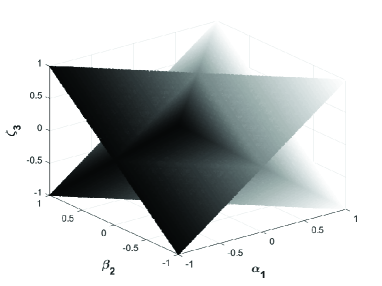
Figure 8: The left image shows a typical $3D$ submanifold of the $\breve{\mathcal{B}}$ family. As seen, a submanifold is smooth and has no topological features. The right figure shows the projection of this manifold on the plane $(\alpha_{1},\zeta_{3})$. Recall that similar pictures arise when we projecting manifold on the plane $(\alpha_{1},\beta_{2})$ and $(\beta_{2},\zeta_{3})$.

The first family $\breve{\mathcal{A}}$ consists of six submanifolds $\breve{\mathcal{A}}=\overline{\breve{\mathcal{A}}_{1},\,\breve{\mathcal{A}}_{6}}$ (see FIG. 7).

Figure 9: The left image shows a typical $3D$ submanifold of the $\breve{\mathcal{C}}$ family that has a topology. The right figure shows the projection of this submanifold on the plane $(\alpha_{1},\beta_{1})$. Recall that the projections of the submanifold on the plane $(\beta_{1},\beta_{2})$ and $(\alpha_{1},\beta_{2})$ do not contain topologies.

Figure 10: The left image shows a typical $3D$ submanifold of the $\breve{\mathcal{D}}$ family that has a topology. The right figure shows the projection of this submanifold on the plane $(\alpha_{1},\alpha_{2})$. Recall that the projections of the submanifold on the plane $(\alpha_{2},\beta_{3})$ and $(\alpha_{1},\beta_{3})$ do not contain topologies.

We can combine the submanifolds of this family similarly to the family of sets and form $3D$ - manifold immersed in the space $\mathbb{R}^{9}$:

$$\mathfrak{S}^{(3)}_{\breve{\mathcal{A}}}=\bigcup_{\alpha\in{\breve{\mathcal{A}}}}\mathfrak{S}^{(3)}_{\alpha}=\bigl{\{}\{\mathcal{x}\}|\,\exists\,\alpha\in{\breve{\mathcal{A}}},\,\{\mathfrak{x}\}\in{\breve{\mathcal{A}}}\bigr{\}},$$ (109)

where $\{\mathfrak{x}\}=\bigl{[}(\alpha_{1},\alpha_{2},\alpha_{3}),(\beta_{1},\beta_{2},\beta_{3}),(\zeta_{1},\zeta_{2},\zeta_{3}),(\alpha_{1},\beta_{1},\zeta_{1}),(\alpha_{2},\beta_{2},\zeta_{2}),(\alpha_{3},\beta_{3},\zeta_{3})\bigr{]}.$

The second family of $\breve{\mathcal{B}}$ also consists of six submanifolds $\breve{\mathcal{B}}=\overline{\breve{\mathcal{B}}_{1},\,\breve{\mathcal{B}}_{6}}$ (see FIG. 8). The united manifold in this case has the form:

$$\mathfrak{S}^{(3)}_{\breve{\mathcal{B}}}=\bigcup_{\alpha\in{\breve{\mathcal{B}}}}\mathfrak{S}^{(3)}_{\alpha}=\bigl{\{}\{\mathfrak{y}\}|\,\exists\,\alpha\in{\breve{\mathcal{B}}},\,\{\mathfrak{y}\}\in{\breve{\mathcal{B}}}\bigr{\}},$$ (110)

where $\{\mathfrak{y}\}=\bigl{[}(\alpha_{1},\beta_{2},\zeta_{3}),(\alpha_{1},\beta_{3},\zeta_{2}),(\alpha_{2},\beta_{3},\zeta_{1}),(\alpha_{2},\beta_{1},\zeta_{3}),(\alpha_{3},\beta_{1},\zeta_{2}),(\alpha_{3},\beta_{2},\zeta_{1})\bigr{]}.$

The third $\breve{\mathcal{C}}=\overline{\breve{\mathcal{C}}_{1},\,\breve{\mathcal{C}}_{36}}$ and fourth $\breve{\mathcal{D}}=\overline{\breve{\mathcal{D}}_{1},\,\breve{\mathcal{D}}_{36}}$ families (see FIG. 9 and FIG. 10), each of which individually consists of 36 submanifolds, can be combined similarly to the previous cases. In particular:

$$\mathfrak{S}^{(3)}_{\breve{\mathcal{G}}}=\bigcup_{\alpha\in{\breve{\mathcal{G}}}}\mathfrak{S}^{(3)}_{\alpha}=\bigl{\{}\{\mathfrak{t}\}|\,\exists\,\alpha\in{\breve{\mathcal{G}}},\,\{\mathfrak{t}\}\in{\breve{\mathcal{G}}}\bigr{\}},$$ (111)

where ${\breve{\mathcal{G}}}=({\breve{\mathcal{C}}},{\breve{\mathcal{D}}})$ and $\{\mathfrak{t}\}=\bigl{(}\{\mathfrak{u}\},\{\mathfrak{v}\}\bigr{)}$, in addition:

$$\{\mathfrak{u}\}=\bigl{[}(\alpha_{1},\alpha_{2},\beta_{3}),(\beta_{3},\zeta_{1},\zeta_{2}),(\beta_{2},\zeta_{1},\zeta_{3}),(\beta_{2},\beta_{3},\zeta_{1}),(\beta_{1},\zeta_{2},\zeta_{3}),(\beta_{1},\beta_{3},\zeta_{2}),(\beta_{1},\beta_{2},\zeta_{3}),$$

$$\quad\qquad(\alpha_{3},\zeta_{1},\zeta_{2}),(\alpha_{3},\beta_{3},\zeta_{2}),(\alpha_{3},\beta_{3},\zeta_{1}),(\alpha_{3},\beta_{2},\zeta_{3}),(\alpha_{3},\beta_{2},\zeta_{2}),(\alpha_{3},\beta_{1},\zeta_{3}),(\alpha_{3},\beta_{1},\zeta_{1}),$$

$$\qquad\quad(\alpha_{3},\beta_{1},\zeta_{2}),(\alpha_{2},\zeta_{1},\zeta_{3}),(\alpha_{2},\beta_{3},\zeta_{3}),(\alpha_{2},\beta_{3},\zeta_{2}),(\alpha_{2},\beta_{2},\zeta_{3}),(\alpha_{2},\beta_{2},\zeta_{1}),(\alpha_{2},\beta_{1},\zeta_{2}),$$

$$\qquad\quad(\alpha_{2},\beta_{1},\zeta_{1}),(\alpha_{2},\beta_{1},\beta_{3}),(\alpha_{2},\alpha_{3},\zeta_{1}),(\alpha_{2},\alpha_{3},\beta_{1}),(\alpha_{1},\zeta_{2},\zeta_{3}),(\alpha_{1},\beta_{3},\zeta_{3}),(\alpha_{1},\beta_{3},\zeta_{1}),$$

$$\quad\qquad(\alpha_{1},\beta_{2},\zeta_{2}),(\alpha_{1},\beta_{2},\zeta_{1}),(\alpha_{1},\beta_{2},\beta_{3}),(\alpha_{1},\beta_{1},\zeta_{3}),(\alpha_{1},\beta_{1},\zeta_{2}),(\alpha_{1},\alpha_{3},\zeta_{2}),(\alpha_{1},\alpha_{3},\beta_{2}),$$

$$(\alpha_{1},\alpha_{2},\zeta_{3})\bigr{]},$$

and

$$\{\mathfrak{v}\}=\bigl{[}(\alpha_{1},\beta_{1},\beta_{2}),\,(\alpha_{1},\alpha_{2},\beta_{2}),\,(\alpha_{1},\alpha_{2},\beta_{1}),(\beta_{3},\zeta_{2},\zeta_{3}),(\beta_{3},\zeta_{1},\zeta_{3}),(\beta_{2},\zeta_{2},\zeta_{3}),(\beta_{2},\zeta_{1},\zeta_{2}),$$

$$\quad\qquad(\beta_{2},\beta_{3},\zeta_{3}),\,(\beta_{2},\beta_{3},\zeta_{2}),\,(\beta_{1},\zeta_{1},\zeta_{3}),\,(\beta_{1},\zeta_{1},\zeta_{2}),\,(\beta_{1},\beta_{3},\zeta_{3}),\,(\beta_{1},\beta_{3},\zeta_{1}),(\beta_{1},\beta_{2},\zeta_{2}),$$

$$\qquad\quad(\beta_{1},\beta_{2},\zeta_{1}),\,(\alpha_{3},\zeta_{2},\zeta_{3}),\,(\alpha_{3},\zeta_{1},\zeta_{3}),\,(\alpha_{3},\beta_{2},\beta_{3}),\,(\alpha_{3},\beta_{1},\beta_{3}),(\alpha_{2},\zeta_{2},\zeta_{3}),\,(\alpha_{2},\zeta_{1},\zeta_{2}),$$

$$\qquad\quad(\alpha_{2},\beta_{2},\beta_{3}),(\alpha_{2},\beta_{1},\beta_{2}),(\alpha_{2},\alpha_{3},\zeta_{3}),(\alpha_{2},\alpha_{3},\zeta_{2}),(\alpha_{2},\alpha_{3},\beta_{3}),(\alpha_{2},\alpha_{3},\beta_{2}),(\alpha_{1},\zeta_{1},\zeta_{3}),$$

$$\quad\qquad(\alpha_{1},\zeta_{1},\zeta_{2}),(\alpha_{1},\beta_{1},\beta_{3}),(\alpha_{1},\alpha_{3},\zeta_{3}),(\alpha_{1},\alpha_{3},\zeta_{1}),(\alpha_{1},\alpha_{3},\beta_{3}),(\alpha_{1},\alpha_{3},\beta_{1}),(\alpha_{1},\alpha_{2},\zeta_{2}),$$

$$(\alpha_{1},\alpha_{2},\zeta_{1})\bigr{]}.$$

Finally, we can combine all the manifolds and find the $3D$ manifold that is immersed in the configuration space $9D$:

$$\mathfrak{S}^{(3)}=\bigcup_{\alpha\in(\breve{\mathcal{A}},\breve{\mathcal{B}},\breve{\mathcal{C}},\breve{\mathcal{D}})}\mathfrak{S}^{(3)}_{\alpha}=\bigl{\{}\{\mathfrak{l}\}|\,\exists\,\alpha\in({\breve{\mathcal{A}}},{\breve{\mathcal{B}}},{\breve{\mathcal{C}}},{\breve{\mathcal{D}}}),\,\{\mathfrak{l}\}\in({\breve{\mathcal{A}}},{\breve{\mathcal{B}}},{\breve{\mathcal{C}}},{\breve{\mathcal{D}}})\bigr{\}},$$ (112)

where $\{\mathfrak{l}\}=\bigl{(}\{\mathfrak{x}\},\{\mathfrak{y}\},\{\mathfrak{u}\},\{\mathfrak{v}\}\bigr{)}.$

XIII.3

Since the existence of inverse coordinate transformations is very important for the proof of the proposition, we now consider the system of algebraic equations (35).

Let us make the following notations:

$$\bar{\alpha}_{\mu}=x^{1}_{\,\,,\,\mu},\quad\bar{\beta}_{\mu}=x^{2}_{\,\,,\,\mu},\quad\bar{\zeta}_{\mu}=x^{3}_{\,\,,\,\mu},\quad\bar{u}_{\mu}=x^{4}_{\,\,,\,\mu},\quad\bar{v}_{\mu}=x^{5}_{\,\,,\,\mu},\quad\bar{w}_{\mu}=x^{6}_{\,\,,\,\mu}.$$ (113)

In addition, we require the following conditions to be fulfilled:

$$\bar{\alpha}_{4}=\bar{\alpha}_{5}=\bar{\alpha}_{6}=0,\quad\bar{\beta}_{4}=\bar{\beta}_{5}=\bar{\beta}_{6}=0,\quad\bar{\zeta}_{4}=\bar{\zeta}_{5}=\bar{\zeta}_{6}=0,\,$$

$$\bar{u}_{1}=\bar{u}_{2}=\bar{u}_{3}=0,\quad\bar{v}_{1}=\bar{v}_{2}=\bar{v}_{3}=0,\quad\bar{w}_{1}=\bar{w}_{2}=\bar{w}_{3}=0.$$ (114)

Now, performing similar arguments and calculations, as in the case of direct coordinate transformations, from (35) it is easy to get the following two systems of algebraic equations:

$$\bar{\alpha}_{1}^{2}+\bar{\beta}_{1}^{2}+\bar{\zeta}_{1}^{2}=\frac{1}{{g}(\{\bar{x}\})},\qquad\bar{\alpha}_{1}\bar{\alpha}_{2}+\bar{\beta}_{1}\bar{\beta}_{2}+\bar{\zeta}_{1}\bar{\zeta}_{2}=0,$$

$$\bar{\alpha}_{2}^{2}+\bar{\beta}_{2}^{2}+\bar{\zeta}_{2}^{2}=\frac{1}{{g}(\{\bar{x}\})},\qquad\bar{\alpha}_{1}\bar{\alpha}_{3}+\bar{\beta}_{1}\bar{\beta}_{3}+\zeta_{1}\zeta_{3}=0,$$

$$\bar{\alpha}_{3}^{2}+\bar{\beta}_{3}^{2}+\bar{\zeta}_{3}^{2}=\frac{\zeta^{33}}{{g}(\{\bar{x}\})},\qquad\bar{\alpha}_{2}\bar{\alpha}_{3}+\bar{\beta}_{2}\bar{\beta}_{3}+\bar{\zeta}_{2}\zeta_{3}=0,$$ (115)

and, correspondingly:

$$\bar{u}_{4}^{2}+\bar{v}_{4}^{2}+\bar{w}_{4}^{2}=\gamma^{44}{g}^{-1}(\{\bar{x}\}),\qquad\bar{u}_{4}\bar{u}_{5}+\bar{v}_{4}\bar{v}_{5}+\bar{w}_{4}\bar{w}_{5}=\gamma^{45}{g}^{-1}(\{\bar{x}\}),$$

$$\bar{u}_{5}^{2}+\bar{v}_{5}^{2}+\bar{w}_{5}^{2}=\gamma^{55}{g}^{-1}(\{\bar{x}\}),\qquad\bar{u}_{4}\bar{u}_{6}+\bar{v}_{4}\bar{v}_{6}+\bar{w}_{4}\bar{w}_{6}=\gamma^{46}{g}^{-1}(\{\bar{x}\}),$$

$$\bar{u}_{6}^{2}+\bar{v}_{6}^{2}+\bar{w}_{6}^{2}=\gamma^{66}{g}^{-1}(\{\bar{x}\}),\qquad\bar{u}_{5}\bar{u}_{6}+\bar{v}_{5}\bar{v}_{6}+\bar{w}_{5}\bar{w}_{6}=\gamma^{56}{g}^{-1}(\{\bar{x}\}),$$ (116)

where $f^{-1}:g(\{\bar{x}\})\mapsto\breve{g}(\{\bar{\rho}\})$.
In particular, systems of algebraic equations (115) and (116), as in the case direct coordinate transformations (see (38) and (39)), generate two 3$D$ manifolds $\bar{\mathfrak{S}}^{(3)}$ and $\bar{\mathfrak{R}}^{(3)}$, respectively.

Thus, we have proved that there are also inverse coordinate transformations.

XIII.4

As mentioned (see (43)), the vector X consists of 18 independent components. Its transposed form looks like this:

$$\textbf{X}^{T}=\bigl{(}\alpha_{11},\alpha_{12},\alpha_{13},\alpha_{22},\alpha_{23},\alpha_{33},\beta_{11},\beta_{12},\beta_{13},\beta_{22},\beta_{23},\beta_{33},\zeta_{11},\zeta_{12},\zeta_{13},\zeta_{22},\zeta_{23},\zeta_{33}\bigr{)}.$$

Taking into account the form of the vector X, we can write the explicit form of the basic matrix:

$$\mathbb{A}=\left(\begin{array}[]{cccccccccccccccccc}d_{\,1}^{\,1}&0&0&0&0&0&d_{\,1}^{\,7}&0&0&0&0&0&d_{\,1}^{13}&0&0&0&0&0\\ 0&d_{\,2}^{\,2}&0&0&0&0&0&d_{\,2}^{\,8}&0&0&0&0&0&d_{\,2}^{14}&0&0&0&0\\ 0&0&d_{\,3}^{\,3}&0&0&0&0&0&d_{\,3}^{\,9}&0&0&0&0&0&d_{\,3}^{15}&0&0&0\\ 0&d_{\,4}^{\,2}&0&0&0&0&0&d_{\,4}^{\,8}&0&0&0&0&0&d_{\,4}^{14}&0&0&0&0\\ 0&0&0&d_{\,5}^{\,4}&0&0&0&0&0&d_{\,5}^{10}&0&0&0&0&0&d_{\,5}^{16}&0&0\\ 0&0&0&0&d_{\,6}^{\,5}&0&0&0&0&0&d_{\,6}^{11}&0&0&0&0&0&d_{\,6}^{17}&0\\ 0&0&d_{\,7}^{\,3}&0&0&0&0&0&d_{\,7}^{\,9}&0&0&0&0&0&d_{\,7}^{15}&0&0&0\\ 0&0&0&0&d_{\,8}^{\,5}&0&0&0&0&0&d_{\,8}^{11}&0&0&0&0&0&d_{\,8}^{17}&0\\ 0&0&0&0&0&d_{9}^{\,6}&0&0&0&0&0&d_{\,9}^{12}&0&0&0&0&0&d_{\,9}^{18}\\ d_{10}^{\,1}&d_{10}^{\,2}&0&0&0&0&d_{10}^{\,7}&d_{10}^{\,8}&0&0&0&0&d_{10}^{13}&0&0&0&d_{10}^{17}&0\\ 0&d_{11}^{\,2}&0&d_{11}^{\,4}&0&0&0&d_{11}^{\,8}&0&d_{11}^{10}&0&0&0&d_{11}^{14}&0&d_{11}^{16}&0&0\\ 0&0&d_{12}^{\,3}&0&d_{12}^{\,5}&0&0&0&d_{12}^{\,9}&0&d_{12}^{11}&0&0&0&d_{12}^{15}&0&d_{12}^{17}&0\\ d_{13}^{\,1}&0&d_{13}^{\,3}&0&0&0&d_{13}^{\,7}&0&d_{13}^{\,9}&0&0&0&d_{13}^{13}&0&d_{13}^{15}&0&0&0\\ 0&d_{14}^{\,2}&0&0&d_{14}^{5}&0&0&d_{14}^{\,8}&0&0&d_{14}^{11}&0&0&d_{14}^{14}&0&0&d_{14}^{17}&0\\ 0&0&d_{15}^{\,3}&0&0&d_{15}^{\,6}&0&0&d_{15}^{\,9}&0&0&d_{15}^{12}&0&0&d_{15}^{15}&0&0&d_{15}^{18}\\ 0&d_{16}^{\,2}&d_{16}^{\,3}&0&0&0&0&d_{16}^{\,8}&d_{16}^{\,9}&0&0&0&0&d_{16}^{14}&d_{16}^{15}&0&0&0\\ 0&0&0&d_{17}^{\,4}&d_{17}^{5}&0&0&0&0&d_{17}^{10}&d_{17}^{11}&0&0&0&0&d_{17}^{16}&d_{17}^{17}&0\\ 0&0&0&0&d_{18}^{\,5}&d_{18}^{\,6}&0&0&0&0&d_{18}^{11}&d_{18}^{12}&0&0&0&0&d_{18}^{17}&d_{18}^{18}\\ \end{array}\right),$$ (117)

where the superscript indicates the column number, while the subscript indicates the line number. As for the explicit form of elements $d^{\,\nu}_{\mu}=d_{\mu\nu}$, where $\mu,\nu=\overline{1,18}$, then we can find they by multiplying the basic matrix $\mathbb{A}$ with the vector X (see equation (43)) and comparing with the system of equations (42).

In particular, it is easy to verify these terms are equal:

$$d^{\,1}_{\,1}\,=\,d^{\,2}_{\,2}\,=\,d^{\,3}_{\,3}\,=2d^{\,2}_{\,10}=2d^{\,4}_{11}=2d^{\,5}_{12}=2d^{\,3}_{13}=\,2d^{\,5}_{14}=2d^{\,6}_{15}=2\alpha_{1},\quad\,$$

$$d^{\,2}_{\,4}\,=\,d^{\,4}_{\,5}\,=\,d^{\,5}_{\,6}\,=\,2d^{\,1}_{10}=2d^{\,2}_{11}=2d^{\,3}_{12}=2d^{\,3}_{16}=2d^{\,5}_{17}=2d_{18}^{\,6}=2\alpha_{2},\quad\,$$

$$d^{\,3}_{\,7}\,=\,d^{\,5}_{\,8}\,=\,d^{\,6}_{\,9}\,=\,2d^{\,1}_{13}=2d^{\,2}_{14}=2d^{\,3}_{15}=2d^{\,2}_{16}=2d^{\,4}_{17}=2d^{\,5}_{18}=2\alpha_{3},\quad\,$$

$$d^{\,1}_{\,7}\,=\,d^{\,2}_{\,8}\,=\,d_{\,9}^{\,3}=\,2d^{\,8}_{10}\,=2d^{10}_{11}=2d^{11}_{12}=2d^{\,9}_{13}=2d^{11}_{14}=2d^{12}_{15}=2\beta_{1},\quad\,$$

$$d^{\,8}_{\,4}=d^{10}_{\,5}=d_{11}^{\,6}=2d^{\,7}_{10}=2d^{\,8}_{11}=2d^{\,9}_{12}=2d^{\,9}_{16}\,=2d^{11}_{17}\,=2d^{12}_{18}=2\beta_{2},\quad\,$$

$$d^{\,9}_{\,7}\,=d^{11}_{\,6}=\,d_{12}^{\,6}=2d^{\,7}_{13}=2d^{\,8}_{14}=2d^{\,9}_{15}=2d^{\,8}_{16}=2d^{10}_{17}=2d^{11}_{18}=2\beta_{3},\quad\,$$

$$d^{\,1}_{13}=d^{\,2}_{14}=d_{15}^{\,3}=2d^{17}_{10}=2d^{16}_{11}=2d^{17}_{12}=2d^{15}_{13}=2d^{17}_{14}=2d^{18}_{15}=2\gamma^{33}\zeta_{1},$$

$$d^{14}_{\,4}=d^{16}_{5}=d_{17}^{\,6}=2d^{13}_{\,10}=2d^{14}_{11}=2d^{15}_{12}=2d^{13}_{13}=2d^{14}_{14}=2d^{15}_{15}=2\gamma^{33}\zeta_{2},$$

$$d^{15}_{\,7}=d^{17}_{\,8}=d_{18}^{\,9}=2d^{14}_{16}=2d^{16}_{17}=2d^{17}_{18}=2d^{15}_{16}=2d^{17}_{17}=2d^{18}_{18}=\,2\gamma^{33}\zeta_{3}.$$ (118)

As is known, the algebraic system (42) or (43) does not have a solution in the case when the determinant of the matrix is zero $\det(\mathbb{A})=\det(d_{\mu\nu})=0.$ A class consisting of sets of coefficients $\{\sigma\}$ for which the determinant is zero can be countable and the measure, respectively, will be equal to zero $\mathfrak{W}=\oslash$.

XIII.5

Let us consider third-order matrices $\Delta_{i}(\{\bar{x}\})\,\,(i=\overline{1,3}\,)$, that are included in the solutions of the system of algebraic equations (48):

$$\Delta_{1}=\left|\begin{array}[]{ccc}\delta&2\xi^{1}\xi^{2}&2\xi^{1}\xi^{3}\\ \delta&K_{2}&2\xi^{2}\xi^{3}\\ \delta&2\xi^{2}\xi^{3}&K_{3}\end{array}\right|,\,\,\Delta_{2}=\left|\begin{array}[]{ccc}K_{1}&\delta&2\xi^{1}\xi^{3}\\ 2\xi^{1}\xi^{2}&\delta&2\xi^{2}\xi^{3}\\ 2\xi^{1}\xi^{3}&\delta&K_{3}\end{array}\right|,\,\,\Delta_{3}=\left|\begin{array}[]{ccc}K_{1}&2\xi^{1}\xi^{2}&\delta\\ 2\xi^{1}\xi^{2}&K_{2}&\delta\\ 2\xi^{1}\xi^{3}&2\xi^{2}\xi^{3}&\delta\end{array}\right|.$$ (128)

By calculating these determinants we get:

$$\Delta_{1}(\{\bar{x}\})=\delta\cdot\bigl{\{}K_{2}K_{3}-2\xi^{1}[\xi^{2}K_{3}+\xi^{3}K_{2}]+4\xi^{2}\xi^{3}[\xi^{1}(\xi^{2}+\xi^{3})-\xi^{2}\xi^{3}]\bigr{\}},$$

$$\Delta_{2}(\{\bar{x}\})=\delta\cdot\bigl{\{}K_{1}K_{3}-2\xi^{2}[\xi^{1}K_{3}+\xi^{3}K_{1}]+4\xi^{1}\xi^{3}[\xi^{2}(\xi^{1}+\xi^{3})-\xi^{1}\xi^{3}]\bigr{\}},$$

$$\Delta_{3}(\{\bar{x}\})=\delta\cdot\bigl{\{}K_{1}K_{2}-2\xi^{3}[\xi^{2}K_{1}+\xi^{1}K_{2}]+4\xi^{1}\xi^{2}[\xi^{3}(\xi^{1}+\xi^{2})-\xi^{1}\xi^{2}]\bigr{\}}.$$ (129)

The main determinant $\Delta(\{\bar{x}\})$ (see (56)) is easy to to calculate:

$$\Delta(\{\bar{x}\})=K_{1}K_{2}K_{3}-4\bigl{[}(\xi^{2}\xi^{3})^{2}K_{1}+(\xi^{1}\xi^{3})^{2}K_{2}+(\xi^{1}\xi^{2})^{2}K_{3}\bigl{]}+16(\xi^{1}\xi^{2}\xi^{3})^{2}.$$ (130)

In a coupled system, given the conditions $\ddot{x}^{i}=0\,\,(i=\overline{1,3}\,)$, bodies can have different constant velocities $\xi^{i}=const_{i}\,\,(i=\overline{1,3})$ depending on their mass. To simplify the determinant $\Delta(\{\bar{x}\})$, it is useful to introduce two new parameters; $\alpha=(const_{2})^{2}=(\xi^{2}/\xi^{1})^{2}$ and $\beta=(const_{3})^{2}=(\xi^{3}/\xi^{1})^{2}$, and also notation $(\xi^{1})^{2}=(const_{1})^{2}=y>0$. In addition, we assume that; $(\xi^{1})^{2}\geq[(\xi^{2})^{2},(\xi^{3})^{2}]$, from which follows that parameters $\alpha,\beta\in[0,1]$.

Using these notations, we can represent the expression (130) in the form of a third-order polynomial:

$$\Delta(\{\bar{x}\})=\mathcal{A}y^{3}+\mathcal{B}y^{2}+\mathcal{C}y-\Lambda^{6},$$ (131)

where

$$\mathcal{A}=\bigl{\{}12\alpha^{2}\beta^{2}+(1-\alpha^{2}-\beta^{2})(1+\alpha^{2}-\beta^{2})(1-\alpha^{2}+\beta^{2})+4(\alpha^{2}+\beta^{2})(1+\alpha^{2}\beta^{2})+4(\alpha^{2}-\beta^{2})^{2}\bigr{\}},$$

$$\mathcal{B}=\bigl{\{}1+2(\alpha^{2}+\beta^{2})+(\alpha^{2}+\beta^{2})^{2}\bigr{\}}\Lambda^{2},\qquad\mathcal{C}=-(1+\alpha^{2}+\beta^{2})\Lambda^{4}.$$

Now to eliminate uncertainties like $0/0$ in expressions (49), we need to find the conditions, that is, the parameters $\alpha$ and $\beta$, for which $\Delta(\{\bar{x}\})\sim\delta$, and later $\delta\to 0$.

Let us consider the cubic equation:

$$\Delta(\{\bar{x}\})=0.$$ (132)

To find the roots of the cubic equation (132), it is convenient to use the Vieta trigonometric formula. Recall that the determinant of the equation (132) has the following form:

$$\mathcal{D}=\mathcal{Q}^{3}-\mathcal{R}^{2},$$

where $\mathcal{Q}=\bigl{(}[\mathcal{B}/\mathcal{A}]^{3}-3[\mathcal{C}/\mathcal{A}]\bigr{)}/9$ and $\mathcal{R}=\bigl{(}2[\mathcal{B}/\mathcal{A}]^{2}-9[\mathcal{B}\mathcal{C}/\mathcal{A}^{2}]-27\Lambda^{6}/\mathcal{A}\bigr{)}/54$.
According to the analysis, depending on the values of the parameters $\alpha$ and $\beta$, three cases are possible for determinant $\mathcal{D}$.

Case 1: When $\mathcal{D}>0$, there are three real solutions:

$$y_{1}=-2\sqrt{\mathcal{Q}}\cos(\phi)-\mathcal{B}/(3\mathcal{A}),\qquad\qquad\qquad\qquad\qquad\qquad\qquad\quad\,\,\,$$

$$y_{2}=-2\sqrt{\mathcal{Q}}\cos(\phi+2\pi/3)-\mathcal{B}/(3\mathcal{A}),\qquad\qquad\qquad\qquad\qquad\qquad\,$$

$$y_{3}=-2\sqrt{\mathcal{Q}}\cos(\phi-2\pi/3)-\mathcal{B}/(3\mathcal{A}),\quad\phi=\bigl{[}\arccos(\mathcal{R}/\mathcal{Q}^{3/2})\bigr{]}/3.\,\,$$ (133)

Case 2: When $\mathcal{D}<0$, depending on the sign of the parameter $\mathcal{Q}$, there are three possible solutions.

$\bullet\,\,\mathcal{Q}>0$, there is one real solution:

$$y=-2\mathrm{sgn}(\mathcal{R})|\mathcal{Q}|^{1/2}\cosh(\phi)-\mathcal{B}/(3\mathcal{A}),\quad\phi=\bigr{[}\mathrm{Arch}\bigl{(}|\mathcal{R}|/|\mathcal{Q}|^{3/2}\bigr{)}\bigr{]}/3.$$ (134)

$\bullet\,\,\mathcal{Q}<0$, in this case, the real solution is:

$$y=-2\mathrm{sgn}(\mathcal{R})|\mathcal{Q}|^{1/2}\sinh(\phi)-\mathcal{B}/(3\mathcal{A}),\quad\phi=\bigr{[}\mathrm{Arsh}\bigl{(}|\mathcal{R}|/|\mathcal{Q}|^{3/2}\bigr{)}\bigr{]}/3.$$ (135)

$\bullet\,\,\mathcal{Q}=0$, in this case, the real solution, accordingly, has the form:

$$y=\Bigl{(}{\Lambda^{6}}/{\mathcal{A}}+\bigl{[}{\mathcal{B}/}{3\mathcal{A}}\bigr{]}^{3}\Bigr{)}^{1/3}.$$ (136)

Case 3: When $\mathcal{D}=0$, there are three real solutions, however, two of them coincide:

$$y_{1}=-2\mathcal{R}^{1/3}-\mathcal{B}/(3\mathcal{A}),\qquad y_{2}=y_{3}=\mathcal{R}^{1/3}-\mathcal{B}/(3\mathcal{A}).$$ (137)

Below, as an example, we will analyze case 1, i.e. when $\mathcal{D}>0$.
Taking into account the solutions (133), the determinant $\Delta(\{\bar{x}\})$ can be represented as:

$$\Delta(\{\bar{x}\})=(y-y_{1})(y-y_{2})(y-y_{3}).$$ (138)

Consider solutions (56) near the value:

$$y=y_{1}\pm\delta.$$ (139)

Using (139) and (129)-(130) for solutions (49), we obtain the following expressions:

$$a_{1}(\{\bar{x}\})=\pm\frac{K_{2}K_{3}-2(y_{1}\pm\delta)^{2}[\alpha K_{3}+\beta K_{2}]+4\alpha\beta(y_{1}\pm\delta)^{4}[\alpha+\beta-\alpha\beta]}{(y_{2}-y_{1}\pm\delta)(y_{3}-y_{1}\pm\delta)},$$

$$a_{2}(\{\bar{x}\})=\,\pm\,\frac{K_{1}K_{3}-2\alpha(y_{1}\pm\delta)^{2}[K_{3}\,+\beta K_{1}]+4\beta(y_{1}\pm\delta)^{4}[\alpha-\beta+\alpha\beta]}{(y_{2}-y_{1}\pm\delta)(y_{3}-y_{1}\pm\delta)},$$

$$a_{3}(\{\bar{x}\})=\pm\,\frac{K_{1}K_{2}-2\beta(y_{1}\pm\delta)^{2}[\alpha K_{1}\,+K_{2}]\,+\,4\alpha(y_{1}\pm\delta)^{4}[\beta-\alpha+\alpha\beta]}{(y_{2}-y_{1}\pm\delta)(y_{3}-y_{1}\pm\delta)}.$$ (140)

Now, making the transition to the limit $\delta\to 0$ in the expressions (140) for the coefficients (56), we get clearly defined regular expressions. Assuming that $y_{1}(\{\bar{x}\})=\lambda_{1}=const$, we can generate by this equation 2$D$ surface in the internal space $\mathbb{E}^{3}$, on which the system of equations (48) has a solution. Similarly, we can find solutions of the system of algebraic equations (56) on $2D$ manifolds generated by equations $y_{2}(\{\bar{x}\})=\lambda_{2}=const$ and $y_{3}(\{\bar{x}\})=\lambda_{3}=const$, respectively.

To analyze the problem, of particular interest is the case when all the masses are the same. In this case, obviously, $\alpha=\beta=1$, using which from the equation (131), taking into account (132), it is easy to find the following cubic equation:

$$27y^{3}+9\Lambda^{2}y^{2}-3\Lambda^{4}y-\Lambda^{6}=0,$$ (141)

which can be written as:

$$(3y+\Lambda^{2})^{2}(3y-\Lambda^{2})=0.$$ (142)

From the equation (142) it follows that there is only one real solution:

$$y=\Lambda^{2}(\{\bar{x}\})/3,\quad or\quad\xi^{1}=const_{1}=\Lambda(\{\bar{x}\})/\sqrt{3}.$$ (143)

Finally, using (49), (129)-(130) and (143), we can find the coefficients of algebraic equation (48):

$$a_{1}(\{\bar{x}\})=a_{2}(\{\bar{x}\})=a_{3}(\{\bar{x}\})=\biggl{(}\frac{K-2y}{\Lambda^{2}+3y}\biggr{)}^{2}=1.$$

Solving the second equation in (143) for a specific value of $\xi^{1}=const_{1}$, we can find a 2$D$ surface $\Xi$ on which a restricted three-body system with holonomic connections is localized.

For other cases, also using similar reasoning, we can find surfaces on which configurations with holonomic connections are localized.

XIII.6

The equation for the covariant derivative (60) can be written as:

$$\frac{\mathcal{D}F^{i}}{\mathcal{D}s}=\dot{F}^{i}+Y^{i},\qquad Y^{i}=\Gamma^{i}_{j\,l}(\{\bar{x}\})\dot{x}^{j}F^{l},\qquad\dot{q}=\frac{dq}{ds},\quad i,j,l=\overline{1,3},$$ (144)

where $Y^{i}\in\mathcal{M}^{(3)}$ is a component of the 3$D$ vector.

Using (144), we can calculate the covariant derivative of the second order:

$$\frac{\mathcal{D}^{2}\zeta^{i}}{\mathcal{D}s^{2}}\,=\,\ddot{\zeta}^{i}\,+\,\Gamma^{i}_{j\,l}\dot{x}^{j}\dot{\zeta}^{l}+\dot{Y}^{i}\,+\,\Gamma^{i}_{j\,l}\dot{x}^{j}Y^{l}\,=\,\ddot{\zeta}^{i}\,+\Gamma^{i}_{j\,l}\dot{x}^{j}\dot{\zeta}^{l}\,+\,\frac{d}{ds}\bigl{(}\Gamma^{i}_{j\,l}\dot{x}^{j}\zeta^{l}\bigr{)}\,+\qquad$$

$$\Gamma^{i}_{j\,l}\Gamma^{l}_{k\,p}\dot{x}^{j}\dot{x}^{k}\zeta^{p}=\ddot{\zeta}^{i}+2\Gamma^{i}_{j\,l}\dot{x}^{j}\dot{\zeta}^{l}+\dot{\Gamma}^{i}_{j\,l}\dot{x}^{j}\zeta^{l}+\Gamma^{i}_{j\,l}\ddot{x}^{j}\zeta^{l}+\Gamma^{i}_{j\,l}\Gamma^{l}_{k\,p}\dot{x}^{j}\dot{x}^{k}\zeta^{p}\,\quad$$

$$=\ddot{\zeta}^{i}+2\Gamma^{i}_{j\,l}\dot{x}^{j}\dot{\zeta}^{l}+(\dot{\Gamma}^{i}_{j\,l}\dot{x}^{j}\zeta^{l}-\Gamma^{i}_{j\,l}\Gamma^{j}_{k\,p}\dot{x}^{k}\dot{x}^{p}\zeta^{l}+\Gamma^{i}_{j\,n}\Gamma^{n}_{k\,p}\dot{x}^{j}\dot{x}^{k}\zeta^{p}),\quad$$ (145)

where $k,n,p=\overline{1,3}$. In addition:

$$\Gamma^{i}_{j\,l}=\frac{1}{2}g^{ip}\bigl{(}\partial_{l}g_{pj}+\partial_{j}g_{lp}-\partial_{p}g_{jl}\bigr{)}=-\delta_{l}^{i}a_{j}-\delta_{j}^{i}a_{l}+\delta^{ip}\delta_{jl}a_{p},\quad a_{k}=-\frac{1}{2}\partial_{x_{k}}\ln g,$$ (146)

$$\dot{\Gamma}^{i}_{j\,l}=\frac{d\Gamma^{i}_{j\,l}}{ds}=\frac{1}{2}\dot{g}^{ip}\bigl{(}\partial_{l}g_{pj}+\partial_{j}g_{lp}-\partial_{p}g_{jl}\bigr{)}+\frac{1}{2}{g}^{ip}\bigl{(}\partial_{l}\dot{g}_{pj}+\partial_{j}\dot{g}_{lp}-\partial_{p}\dot{g}_{jl}\bigr{)}\,$$

$$=\frac{1}{g}\Bigl{(}\sum_{k=1}^{3}a_{k}\dot{x}^{k}\Bigr{)}\Bigl{[}\bigl{(}\delta^{i}_{j}a_{l}+\delta^{i}_{p}a_{j}-\delta^{ip}\delta_{j\,l}a_{p}\bigr{)}-\bigl{(}\delta^{i}_{j}b_{l}+\delta^{i}_{p}b_{j}-\delta^{ip}\delta_{jl}b_{p}\bigr{)}\Bigl{]}\,$$

$$=\frac{1}{g}\Bigl{(}\sum_{k=1}^{3}a_{k}\dot{x}^{k}\Bigr{)}\Bigl{[}\bigl{(}\delta^{i}_{j}(a_{l}-b_{l})+\delta^{i}_{p}(a_{j}-b_{j})-\delta^{ip}\delta_{jl}(a_{p}-b_{p})\Bigl{]},$$ (147)

where $b_{k}=-(1/2)\partial_{x_{k}}\ln\bigl{|}\sum_{i=1}^{3}g_{;i}\dot{x}^{i}\bigr{|}$ and $g_{;\,k}=\partial g/\partial x^{k}.$

XIII.7

Substituting (77) into the equation (76), we get:

$$\Biggl{\{}\frac{1}{{\mathrm{r}}^{2}}\frac{\mathrm{d}}{\mathrm{d}\mathrm{r}}\biggl{(}{\mathrm{r}}^{2}\frac{\mathrm{d}}{\mathrm{d}{{\mathrm{r}}}}\biggr{)}-\frac{{l(l+1)}}{{\mathrm{r}}^{2}}+\frac{2}{\hbar^{2}}\sum_{\bar{l}=0}^{\infty}\sum_{\bar{m}=-\bar{l}}^{\bar{l}}\Omega_{\bar{l}\bar{m}}({\mathrm{r}}\,;\,\mathrm{E},J,\varepsilon)Y_{\bar{l}}^{\bar{m}}(\theta,\varphi)\Biggr{\}}\bar{\Psi}=0,$$ (148)

where $\Omega_{\bar{l}\bar{m}}({\mathrm{r}}\,;\,\mathrm{E},J,\varepsilon)=\bigl{[}\mathrm{E}\,\mathfrak{g}^{(1)}_{\bar{l}\bar{m}}(\mathrm{r};\varepsilon)-J(J+1)\mathfrak{g}^{(2)}_{\bar{l}\bar{m}}(\mathrm{r};\varepsilon)\bigr{]}$.

To simplify the equation (148), we first multiply it by the complex conjugate of the spherical function, that is $Y_{l^{\prime}}^{m^{\prime}\ast}(\theta,\varphi)$ then using the well-known orthogonal properties of the spherical functions Hob :

$$\int_{0}^{2\pi}\int_{0}^{\pi}{Y_{l}^{m}(\theta,\varphi){Y_{l^{\prime}}^{m^{\prime}}}^{\ast}(\theta,\varphi)}\sin\theta d\theta d\varphi=\delta_{mm^{\prime}}\delta_{ll^{\prime}},$$

we obtain the following ordinary differential equation (ODE) for the radial component of the wave function:

$$\Biggl{\{}\frac{1}{{\mathrm{r}}^{2}}\frac{\mathrm{d}}{\mathrm{d}\mathrm{r}}\biggl{(}{\mathrm{r}}^{2}\frac{\mathrm{d}}{\mathrm{d}{{\mathrm{r}}}}\biggr{)}-\frac{l(l+1)}{{\mathrm{r}}^{2}}\Biggr{\}}\delta_{mm^{\prime}}\delta_{ll^{\prime}}\,\Upsilon=-\frac{2}{\hbar^{2}}\sum_{\bar{l}=0}^{\infty}\sum_{\bar{m}=-\bar{l}}^{\bar{l}}\mathcal{W}_{m,m^{\prime},\bar{m}\,;\,l,l^{\prime},\bar{l}}\,\Omega_{\bar{l}\bar{m}}({\mathrm{r}};\,\mathrm{E},J)\Upsilon,$$ (149)

where

$$\mathcal{W}_{m_{1},m_{2},m_{3}\,;\,l_{1},l_{2},l_{3}}=\int_{0}^{2\pi}\int_{0}^{\pi}Y_{l_{1}}^{m_{1}}(\theta,\varphi)Y_{l_{2}}^{m_{2}\ast}(\theta,\varphi)Y_{l_{3}}^{m_{3}}(\theta,\varphi)\sin\theta{d\theta}d\varphi.$$

For calculation the integral of the product of three spherical harmonics $\mathcal{W}_{m_{1},m_{2},m_{3}\,;\,l_{1},l_{2},l_{3}}$ we will use the following formula Zar :

$$\int_{0}^{2\pi}\int_{0}^{\pi}Y_{l_{1}m_{1}}(\theta,\varphi)Y_{l_{2}m_{2}}(\theta,\varphi)Y_{l_{3}m_{3}}(\theta,\varphi)\sin\theta{d\theta}d\varphi=\qquad$$

$$\sqrt{\frac{(2l_{1}+1)(2l_{2}+1)(2l_{3}+1)}{4\pi}}\,\biggl{(}\begin{array}[]{ccc}l_{1}&l_{2}&l_{3}\\ 0&0&0\end{array}\biggr{)}\biggl{(}\begin{array}[]{ccc}l_{1}&l_{2}&l_{3}\\ m_{1}&m_{2}&m_{3}\end{array}\biggr{)},$$ (154)

where $Y_{lm}(\theta,\varphi)$ is the real spherical function, which can be represented by a complex spherical function $Y_{l}^{m}(\theta,\varphi)$ (see Hob ) and $\biggl{(}\begin{array}[]{ccc}l_{1}&l_{2}&l_{3}\\ m_{1}&m_{2}&m_{3}\end{array}\biggr{)}$ denotes the Wigner $3j$ symbol (see Wigner ). Using the transform:

$$Y_{l}^{m}(\theta,\varphi)=\left\{\begin{array}[]{ll}\,\,\,\frac{1}{\sqrt{2}}\,\bigl{(}Y_{l|m|}\,-\,iY_{l,-|m|}\bigr{)},&m<0,\\ \,\,\,Y_{0m},&m=0,\\ \frac{(-1)^{m}}{\sqrt{2}}\bigl{(}Y_{l|m|}+iY_{l,-|m|}\bigr{)},&m>0,\end{array}\right.$$

we can calculate the function $\mathcal{W}_{m_{1},m_{2},m_{3}\,;\,l_{1},l_{2},l_{3}}$.

As follows from (149), this equation, depending on the ratios of the quantum numbers $m,m^{\prime},l$ and $l^{\prime}$, can go over into two different equations:

1. Into the algebraic equation:

$$\sum_{\bar{l}=0}^{\infty}\sum_{\bar{m}=-\bar{l}}^{\bar{l}}\mathcal{W}_{m,m^{\prime},\bar{m}\,;\,l,l^{\prime},\bar{l}}\,\Omega_{\bar{l}\bar{m}}({\mathrm{r}};\,\mathrm{E},J,\varepsilon)=0,$$ (155)

when one of the inequalities holds; $m\neq m^{\prime}$ or $l\neq l^{\prime}$, or when take place of both inequalities $m\neq m^{\prime}$ and $l\neq l^{\prime}$, and, accordingly,

2. into the ODE for the radial wave function of bodies system (see (78) ), if $m=m^{\prime}$ and $l=l^{\prime}$.

Note that the algebraic equation (155) generates the discrete set of points $\mathcal{Y}$ at which the wave function is not defined. However, the cardinality of the set $\mathcal{Y}$ with respect to the cardinality of the set that forms the internal space $\mathcal{M}^{(3)}$ is equal to zero. The latter means that the wave function of a dynamical system is defined in the space $\mathcal{M}^{(3)}\setminus\mathcal{Y}.$

Based on this, below we will calculate only those $3j$ symbols that will be needed to determine the ODE for the quantum motion (see (78)).

Case 1. Assuming that $m=m^{\prime}<0$ and $l=l^{\prime}$, as well as taking into account the selection rules for the Wigner $3j$ symbol, we obtain:

$$\mathcal{W}_{m,m,\bar{m};\,l,\,l,\,\bar{l}}=(-1)^{\bar{m}}\frac{2l+1}{4}\sqrt{\frac{2\bar{l}+1}{\pi}}\biggl{(}\begin{array}[]{ccc}l&l&\bar{l}\\ 0&0&0\end{array}\biggr{)}\biggl{(}\begin{array}[]{ccc}l&l&\bar{l}\\ -|m|&-|m|&|\bar{m}|\end{array}\biggr{)},\quad\bar{m}>0,$$ (160)

$$\mathcal{W}_{m,m,\bar{m};\,l,\,l,\,\bar{l}}=\frac{2l+1}{4}\sqrt{\frac{2\bar{l}+1}{\pi}}\biggl{(}\begin{array}[]{ccc}l&l&\bar{l}\\ 0&0&0\end{array}\biggr{)}\biggl{(}\begin{array}[]{ccc}l&l&\bar{l}\\ -|m|&-|m|&|\bar{m}|\end{array}\biggr{)},\quad\bar{m}<0.$$ (165)

It is easy to see that the second $3j$ symbol in (165) is not equal to zero only if the equality $\bar{m}=2m$ holds. Recall that it follows directly from selection rules. From this condition, in particular, it follows that the first and second expressions in (165) are equal.

Case 2. When $m=m^{\prime}>0$ and $l=l^{\prime}$, the Wigner $3j$ symbol is calculated in the same way and gives the result similarly (165).

Case 3. When $\bar{m}=0$, in addition, $m=m^{\prime}$ and $l=l^{\prime}$. For this case we obtain:

$$\mathcal{W}_{0,0,0;\,l,l,\bar{l}}=\frac{2l+1}{2}\sqrt{\frac{2\bar{l}+1}{\pi}}\biggl{(}\begin{array}[]{ccc}l&l&\bar{l}\\ 0&0&0\end{array}\biggr{)}^{2}.$$ (168)

To calculate the $3j$ symbol, we turn to the well-known general representation Ed :

$$\biggl{(}\begin{array}[]{ccc}l_{1}&l_{2}&l_{3}\\ m_{1}&m_{2}&m_{3}\end{array}\biggr{)}=\biggl{[}\frac{(l_{1}+l_{2}-l_{3})!(l_{1}-l_{2}+l_{3})!(-l_{1}+l_{2}+l_{3})!}{(l_{1}+l_{2}+l_{3}+1)!}\biggr{]}^{1/2}\times$$ (171)

$$\bigl{[}(l_{1}+m_{1})!(l_{1}-m_{1})!(l_{2}+m_{2})!(l_{2}-m_{2})!(l_{3}+m_{3})!(l_{3}-m_{3})!\bigr{]}^{1/2}\,\,\times$$

$$\sum_{\nu}\Bigl{\{}\bigl{(}-1\bigr{)}^{\nu+l_{1}-l_{2}-m_{1}}\,\bigl{[}\nu!(l_{1}+l_{2}-l_{3}-\nu)!(l_{1}-m_{1}-\nu)!\,\times$$

$$(l_{2}+m_{2}-\nu)!(l_{3}-l_{1}-m_{2}+\nu)!(l_{3}-l_{2}+m_{1}+\nu)!\bigr{]}^{-1}\Bigr{\}},$$ (172)

where summation over $\nu$ is carried out over all integers.

Using (172) and the selection rules for the Wigner $3j$ symbol, we can calculate the following specific $3j$ symbols:

$$\Biggl{(}\begin{array}[]{ccc}l&l&\bar{l}\\ -|m|&-|m|&|\bar{m}|\end{array}\Biggr{)}\,=\,\biggl{[}\frac{(2l-\bar{l}\,)!(\bar{l}+|\bar{m}|)!(\bar{l}-|\bar{m}|)!}{(2l+\bar{l}+1)!}\biggr{]}^{1/2}\,\bar{l}!\,(l+|m|)!\,(l-|m|)!\times$$ (175)

$$\sum_{\nu}\frac{\bigl{(}-1\bigr{)}^{\nu+|m|}}{\nu!(2l-\bar{l}-\nu)!(l+|m|-\nu)!(l-|m|-\nu)!(\bar{l}-l+|m|+\nu)!(\bar{l}-l-|m|+\nu)!},$$ (176)

and correspondingly:

$$\biggl{(}\begin{array}[]{ccc}l&l&\bar{l}\\ 0&0&0\end{array}\biggr{)}=\biggl{[}\frac{(2l-\bar{l}\,)!}{(2l+\bar{l}+1)!}\biggr{]}^{1/2}\bigl{(}\bar{l}!l!\bigr{)}^{2}\sum_{\nu}\frac{\bigl{(}-1\bigr{)}^{\nu}}{\nu!(2l-\bar{l}-\nu)!\bigl{[}(l-\nu)!(\bar{l}-l+\nu)!\bigr{]}^{2}}.$$ (179)

Based on the above analysis and selection rules for $3j$ symbols, the quantum equation (149) can be written as:

$$\Biggl{\{}\frac{1}{{\mathrm{r}}^{2}}\frac{\mathrm{d}}{\mathrm{d}\mathrm{r}}\biggl{(}{\mathrm{r}}^{2}\frac{\mathrm{d}}{\mathrm{d}{{\mathrm{r}}}}\biggr{)}-\frac{l(l+1)}{{\mathrm{r}}^{2}}\Biggr{\}}\Upsilon=-\frac{2l+1}{\hbar^{2}}\sum_{\bar{l}=\,0}^{2l}\sum_{\bar{m}=\,0}^{\bar{l}}\sqrt{\frac{2\bar{l}+1}{\pi}}\times$$

$$\biggl{(}\begin{array}[]{ccc}l&l&\bar{l}\\ 0&0&0\end{array}\biggr{)}\biggl{(}\begin{array}[]{ccc}l&l&\bar{l}\\ -|m|&-|m|&|\bar{m}|\end{array}\biggr{)}\Omega_{\bar{l}\bar{m}}({\mathrm{r}};\,\mathrm{E},J)\Upsilon.$$ (184)

Note that the upper limit of summation over $\bar{l}$ is the value $2l$. Recall that this fact is related to the selection rules, according to which the symbol $3j$ is not equal to zero, in particular, if $|l-l^{\prime}|\leq\bar{l}\leq l+l^{\prime}$. Since in the case under consideration $l=l^{\prime}$, therefore, $0\leq\bar{l}\leq 2l$.

XIII.8

If we assume that $\zeta=\cos\varphi$, then the second-order derivative $\mathrm{d}^{2}\Theta_{K}^{j}/(\mathrm{d}\varphi)^{2}$ will have the following form:

$$\frac{\mathrm{d}^{2}\Theta^{j}_{K}}{\mathrm{d}\varphi^{2}}=-\zeta\frac{\mathrm{d}\Theta^{j}_{K}}{\mathrm{d}\zeta}+\bigl{(}1-\zeta^{2}\bigr{)}\frac{\mathrm{d}^{2}\Theta^{j}_{K}}{\mathrm{d}\zeta^{2}}=\zeta\frac{\mathrm{d}\Theta^{j}_{K}}{\mathrm{d}\zeta}-\biggl{[}j(j+1)-\frac{K^{2}}{1-\zeta^{2}}\biggr{]}\Theta^{j}_{K}.$$ (185)

Using (185), we can calculate the following integral, which will play an important role in further calculations:

$$\mathbf{Q}_{jKK^{\prime}}=\int_{-1}^{1}\,\Theta^{j}_{K^{\prime}}\frac{\mathrm{d}^{2}\Theta^{j}_{K}}{\mathrm{d}\varphi^{2}}\,\mathrm{d}\zeta=\int_{-1}^{1}\,\zeta\Theta^{j}_{K^{\prime}}\frac{\mathrm{d}\Theta^{j}_{K}}{\mathrm{d}\zeta}\,\mathrm{d}\zeta-\int_{-1}^{1}\biggl{[}j(j+1)-\frac{K^{2}}{1-\zeta^{2}}\biggr{]}\Theta^{j}_{K^{\prime}}\Theta^{j}_{K}\,d\zeta.$$ (186)

Multiplying the equation (88) by the associated Legendre function $\Theta^{j}_{K^{\prime}}\bigl{(}\zeta\bigr{)}$ and integrating it over the variable $\zeta$ in the range $[1,-1]$ we get:

$$\biggl{\{}\delta_{KK^{\prime}}\biggl{[}\frac{1}{\mathrm{\varrho}}\frac{\partial}{\partial\mathrm{\varrho}}\biggl{(}\mathrm{\varrho}\frac{\partial}{\partial\mathrm{\varrho}}\biggr{)}+\frac{\partial^{2}}{\partial z^{2}}\biggr{]}+\frac{\mathbf{Q}_{jKK^{\prime}}}{\mathrm{\varrho}^{2}}+\frac{2\mu_{0}}{\hbar^{2}}\widetilde{\mathbf{\Omega}}_{jKK^{\prime}}\bigl{(}\varrho,z\big{)}\biggr{\}}\widetilde{\Upsilon}=0,$$ (187)

where

$${\mathbf{Q}}_{jKK^{\prime}}=\sum_{m=0}^{\infty}I^{j}_{mKK^{\prime}},\qquad I^{j}_{mKK^{\prime}}=\int_{-1}^{1}\Theta^{j}_{K}\bigl{(}\zeta\bigr{)}\Theta^{j}_{K^{\prime}}\bigl{(}\zeta\bigr{)}\Theta^{0}_{m}\bigl{(}\zeta\bigr{)}d\zeta,$$

$$\widetilde{\mathbf{\Omega}}_{jKK^{\prime}}\bigl{(}\varrho,z\big{)}=\bigl{[}\mathrm{E}\widetilde{\mathfrak{g}}^{\,(1)}_{m}-J(J+1)\widetilde{\mathfrak{g}}^{\,(2)}_{m}\bigr{]}.\qquad\qquad$$ (188)

To calculate the term $I(j,K;j,K^{\prime};0,m)\equiv I^{j}_{mKK^{\prime}}$, we can use the following general formula Mav ; Shi :

$$I(m_{1},j_{1};m_{2},j_{2};m_{3},j_{3})=\qquad\qquad\qquad\qquad\qquad\qquad\qquad\qquad$$

$$\int_{-1}^{+1}\Theta^{m_{1}}_{j_{1}}(x)\Theta^{m_{2}}_{j_{2}}(x)\Theta^{m_{3}}_{j_{3}}(x)dx=\sqrt{\frac{(j_{2}+m_{2})!(j_{1}+m_{1})!}{(j_{2}-m_{2})!(j_{1}-m_{1})!}}\sum_{n}\biggl{[}(-1)^{m_{1}+m_{2}}(2n+1)\times\quad$$

$$\biggl{(}\begin{array}[]{ccc}j_{1}&j_{2}&n\\ 0&0&0\end{array}\biggr{)}\biggl{(}\begin{array}[]{ccc}j_{1}&j_{2}&n\\ m_{1}&m_{2}&-m_{1}-m_{2}\end{array}\biggr{)}\sqrt{\frac{(n-m_{1}-m_{2})!}{(n+m_{1}+m_{2})!}}\int_{-1}^{+1}\Theta^{m_{3}}_{j_{3}}(x)\Theta^{m_{1}+m_{2}}_{n}(x)dx\biggr{]},\quad$$ (193)

where it is assumed that; $j_{1}+m_{1}+j_{2}+m_{2}+j_{3}+j_{3},$ is even in addition, also are even $|j_{1}-j_{2}|\leq n\leq j_{1}+j_{2},\,j_{1}+j_{2}+n$ and $n+m_{1}+m_{2}+m_{3}+j_{3}$. As for the integral from two associated Legendre polynomials, it is calculated exactly for an arbitrary case:

$$\int_{-1}^{+1}\Theta^{m_{1}}_{j_{1}}(x)\Theta^{m_{2}}_{j_{2}}(x)dx=\frac{(-1)^{m_{2}}2^{-2|m_{2}-m_{1}|-1}\pi}{\Gamma(1/2+|m_{2}-m_{1}|/2)\Gamma(3/2+|m_{2}-m_{1}|/2)}\,\times$$

$$\sqrt{\frac{(j_{1}+m_{1})!(m_{2}+j_{2})!}{(j_{1}-m_{1})!(m_{2}-j_{2})!}}\sum_{k}G_{\{\bullet\}}\bigl{(}1+(-1)^{k+|m_{2}-m_{1}|}\bigr{)}\sqrt{\frac{(k+|m_{2}-m_{1}|)!}{(k-|m_{2}-m_{1}|)!}}\,\times$$

$$\frac{\Gamma(1/2)\Gamma(k/2)\Gamma(|m_{2}-m_{1}|+1)\Gamma(-[k+1]/2)}{\Gamma([|m_{2}-m_{1}|+1-k]/2)\Gamma(|m_{2}-m_{1}|/2)\Gamma([|m_{2}-m_{1}|+k]/2+1)\Gamma(-[|m_{2}-m_{1}|-1]/2)},$$

where again $|j_{2}-j_{1}|\leq k\leq j_{2}+j_{1}$ and $k+j_{1}+j_{2}$ are even. Additionally one requires that the integrand is even, i.e. $j_{1}+m_{1}+j_{2}+m_{2}=even.$ As for the function $G_{\{\bullet\}}$, then it is defined by the help of $3j$ symbols as:

$$G_{\{\bullet\}}=(-1)^{-m_{1}+m_{2}}(2k+1)\biggl{(}\begin{array}[]{ccc}j_{1}&j_{2}&j_{3}\\ 0&0&0\end{array}\biggr{)}\biggl{(}\begin{array}[]{ccc}j_{1}&j_{2}&k\\ -m_{1}&m_{2}&m_{1}-m_{2}\end{array}\biggr{)}.$$

From the equation (187) in the case $K\neq K^{\prime}$ we obtain the following algebraic equation:

$$\frac{\mathbf{Q}_{jKK^{\prime}}}{\mathrm{\varrho}^{2}}+\frac{2\mu_{0}}{\hbar^{2}}\widetilde{\mathbf{\Omega}}_{jKK^{\prime}}\bigl{(}\varrho,z\big{)}=0.$$ (194)

The set of points $\mathcal{Z}$ that generates the equation (194) with respect to the set of points forming the internal space $\mathcal{M}^{(3)}$ has power zero. Recall that the wave function is not uniquely determined on the set of points $\mathcal{Z}$, i.e. it can be defined in the space $\mathcal{M}^{(3)}\setminus\mathcal{Z}$.

We now turn to the question of obtaining an equation whose solution in the limit $z\to+\infty$ goes over to the $\mathbf{S}$ -matrix elements. For this, we substitute the full wave function of the three-body system (99) into the Schrödinger equation (85):

$$\sum_{\bar{n}\bar{j}}\biggl{\{}\frac{1}{\mathrm{\varrho}}\frac{\partial}{\partial\mathrm{\varrho}}\biggl{(}\mathrm{\varrho}\frac{\partial}{\partial\mathrm{\varrho}}\biggr{)}+\frac{\partial^{2}}{\partial z^{2}}+\frac{1}{\mathrm{\varrho}^{2}}\frac{\partial^{2}}{\partial\varphi^{2}}+\frac{2\mu_{0}}{\hbar^{2}}\widetilde{\Omega}\bigl{(}\{\bar{\varrho}\}\bigr{)}\biggr{\}}\mathbf{\Xi}^{+(J)}_{[\mathcal{K}]\,[\bar{\mathcal{K}}]}(z)\Pi_{\bar{n}(\bar{j}\bar{K})}(\varrho;z)\Theta_{\bar{K}}^{\bar{j}}(\zeta)=0,$$ (195)

where $\mathbf{\Xi}^{+(J)}_{[\mathcal{K}]\,[\bar{\mathcal{K}}]}(z)$ and $\Pi_{\bar{n}(\bar{j}\bar{K})}(\varrho;z)$ functions that still need to be defined.

Multiplying the equation (195) by the associated Legendre function $\Theta^{j}_{K^{\prime}}\bigl{(}\zeta\bigr{)}$ and integrating it over the variable $\zeta$ in the range $[1,-1]$, taking into account the condition of orthogonality of these functions, we obtain:

$$\sum_{\bar{n}\bar{j}}\biggl{\{}\delta_{j^{\,{}^{\prime}}\bar{j}}\,\delta_{K^{\prime}\bar{K}}\biggl{[}\frac{1}{\mathrm{\varrho}}\frac{\partial}{\partial\mathrm{\varrho}}\biggl{(}\mathrm{\varrho}\frac{\partial}{\partial\mathrm{\varrho}}\biggr{)}+\frac{\partial^{2}}{\partial z^{2}}\biggr{]}+\frac{\mathbf{Q}_{j^{\,{}^{\prime}}\bar{j}K^{\prime}\bar{K}}}{\mathrm{\varrho}^{2}}+\frac{2\mu_{0}}{\hbar^{2}}\widetilde{\mathbf{\Omega}}_{j^{\,{}^{\prime}}\bar{j}K^{\prime}\bar{K}}\bigl{(}\varrho,z\big{)}\biggr{\}}\mathbf{\Xi}^{+(J)}_{[\mathcal{K}]\,[\bar{\mathcal{K}}]}(z)\Pi_{\bar{n}(\bar{j}\bar{K})}(\varrho;z)=0.$$ (196)

Let us consider the following reference equation:

$$\biggl{\{}\frac{1}{\mathrm{\varrho}}\frac{\partial}{\partial\mathrm{\varrho}}\biggl{(}\mathrm{\varrho}\frac{\partial}{\partial\mathrm{\varrho}}\biggr{)}+\frac{\mathbf{Q}_{j^{\,{}^{\prime}}\bar{j}K^{\prime}\bar{K}}}{\mathrm{\varrho}^{2}}+\frac{2\mu_{0}}{\hbar^{2}}\widetilde{\mathbf{\Omega}}_{j^{\,{}^{\prime}}\bar{j}K^{\prime}\bar{K}}\bigl{(}\varrho,z\big{)}\biggr{\}}\Pi_{\bar{n}(\bar{j}\bar{K})}(\varrho;z)=\mathcal{E}^{(j^{\,{}^{\prime}}K^{\prime})}_{\bar{n}(\bar{j}\bar{K})}(z)\Pi_{\bar{n}(\bar{j}\bar{K})}(\varrho;z),$$ (197)

which is actually a parametric, second-order ODE.

Based on the fact that the localization of the quantum current occurs near the coordinate $z$ by the coordinate $\varrho$, it can be assumed that the solution $\Pi_{\bar{n}(\bar{j}\bar{K})}(\varrho;z)$ is quantized. In other words, the solutions $\Pi_{\bar{n}(\bar{j}\bar{K})}(\varrho;z)$ form an orthonormal basis in a Hilbert space, and we can write the following condition of orthonormality:

$$\int_{0}^{\infty}\Pi_{n(jK)}(\varrho;z){\Pi^{\ast}_{\bar{n}(\bar{j}\bar{K})}(\varrho;z)}d\varrho=\delta_{n\bar{n}}.$$

Finally, multiplying the equation (197) by the solution ${\Pi_{n^{\prime}(j^{\,{}^{\prime}}K^{\prime})}(\varrho;z)}^{\ast}$ and integrating, we obtain the following ODE :

$$\sum_{\bar{n}\bar{j}}\delta_{n^{\prime}\bar{n}}\biggl{\{}\delta_{j^{\,{}^{\prime}}\bar{j}}\,\delta_{K^{\prime}\bar{K}}\frac{\mathrm{d}^{2}}{\mathrm{d}z^{2}}+\overline{\mathcal{E}}^{\,n^{\prime}(j^{\,{}^{\prime}}K^{\prime})}_{\bar{n}(\bar{j}\bar{K})}(z)\biggr{\}}\mathbf{\Xi}^{+(J)}_{[\mathcal{K}]\,[\bar{\mathcal{K}}]}(z)=0,$$ (198)

where $\overline{\mathcal{E}}^{\,n^{\prime}(j^{\,{}^{\prime}}K^{\prime})}_{\bar{n}(\bar{j}\bar{K})}(z)=\int_{0}^{\infty}\Pi_{n^{\prime}(j^{\,{}^{\prime}}K^{\prime})}(\varrho;z)\mathcal{E}^{(j^{\,{}^{\prime}}K^{\prime})}_{\bar{n}(\bar{j}\bar{K})}(z){\Pi^{\ast}_{\bar{n}(\bar{j}\bar{K})}(\varrho;z)}d\varrho.$

The equation (198) at the $n^{\prime}=\bar{n},\,j^{\,{}^{\prime}}=\bar{j}$ and $K=K^{\prime}$ takes the simple form of the second -order ODE (see equation (100)).

In the case when at least one pair of quantum numbers does not coincide between two sets $[\mathcal{K}^{\prime}]$ and $[\bar{\mathcal{K}}]$, from (198) we obtain the algebraic equations:

$$\sum_{\bar{j}}\overline{\mathcal{E}}^{\,n^{\prime}(j^{\,{}^{\prime}}K^{\prime})}_{\,\bar{n}\,(\bar{j}\,\,\bar{K})}(z)=0,\qquad n^{\prime}\neq\bar{n}\quad or\quad K\neq\bar{K}.$$ (199)

The algebraic equation (199) generates a line on which the function should be equal to zero. Note that this is an additional condition imposed on the function $\mathcal{E}_{\,\bar{n}\,(\bar{j}\,\,\bar{K})}(z)$.

References

References

• (1) Poincaré, H. New Methods of Celestial Mechanics, Volume 1, Chapter 1, American Institute of Physics (1993).
• (2) Whittaker, E.T., A Treatise on the Analytical Dynamicals of Particles and Rigid Bodies. With an Introduction to the Problem of Three Bodies, University Press in Cambridge (1988).
• (3) Chenciner, A. Poincaré and the Three-Body Problem, Poincaré, 1912-2012, Séminaire Poincaré XVI, 45-133 (2012).
• (4) Valtonen, M. and Karttunen, H., The Three-Body Problem (Cambridge University Press, Cambridge, 2005).
• (5) Lin, F.J., Symplectic reduction, geometric phase, and internal dynamicals in three-body molecular dynamicals, Phys. Lett. A, 234, 291-300 (1997).
• (6) Lemaître, G., The Three-Body Problem, NASA CR-110 (1964). Available at NASA technical report server http://ntrs.nasa.gov/
• (7) Bruns, E.H., Über die Integrale des Vielekörperproblems Acta Math., 11, 25 (1887).
• (8) Arnold, V.I., Kozlov, V.V. and Neishtadt, A.I., Mathematical Aspects of Classical and Celestial Mechanics, 3rd ed., Dynamical Systems III, Encyclopaedia of Mathematical Sciences, 3, Springer (2006).
• (9) Marchal, C., The three-body problem, Elsevier (2006).
• (10) Bruno, A.D., The restricted three-body problem: Plane Periodic Orbits, de Gruyter (1994).
• (11) Šuvakov, M. and Dmitrašinovič, V., Three Classes of Newtonian Three-Body Planar Periodic Orbits, Phys. Rev. Lett. 110, 114301.
• (12) Li, X. and Liao, S., More than six hundred new families of Newtonian periodic planar collisionless three-body orbits, Sci. China Phys. Mech. Astron. (2017) 60: 129511. https://doi.org/10.1007/s11433-017-9078-5.
• (13) Orlov, V., Titov, V. and Shombina, L., Astronomy Reports, 60, 1083 (2016).
• (14) Li, X., Jing, Y. and Liao, S., Over a thousand new periodic orbits of a planar three-body system with unequal masses, Publ. Astron. Soc. Japan, (2018), 70(4), 64 (1-7). doi: 10.1093/pasj/psy057
• (15) Herschbach, D.R., Reactive collisions in crossed molecular beams, Discuss. Faraday Soc., 33, 149-161 (1962).
• (16) Levine, R.D. and Bernstein, R.B., Molecular Reaction Dynamicals and Chemical Reactivity, Oxford University Press, New York, 1987.
• (17) Cross, R.J. and Herschbach, D.R., Classical scattering of an atom from a diatomic rigid rotor, J. Chem. Phys., 43, 3530-3540 (1965).
• (18) Guichardet, A., On rotation and vibration motions of molecules, Ann. Inst. H. Poincaré, Phys. Tháor., 40, 329-342, (1984).
• (19) Iwai, T., A geometric setting for classical molecular dynamicals, Ann. Inst. H. Poincaré, Phys. Tháor., 47, 199-219 (1987).
• (20) Lin, F.J., Hamiltonian dynamics of atom-diatomic molecular complexes and collisions, Disc. Cont. Dyn. Sys. Suppl., 655-666, (2007). Website: www.AIMSciences.org
• (21) Kryulov, N.S., Foundations of Statistical Physics, 283, Princeton University Press: Princeton and Guildford, UK, 1980.
• (22) Savvidy, G.K., The Yang-Mills classical mechanics as a Kolmogorov K-system, Phys. Lett. B., 130 (5), 303-307 (1983).
• (23) Gurzadian, V.G. and Savvidy, G.K., On Problem of Relaxation of Stellar System, Dokl. AN SSSR. 277 (1), 69-73 (1984).
• (24) Gurzadian, V.G. and Savvidy, G.K., Collective Relaxation of Stellar Systems, Astron. Astrophys. 160, 203-210 (1986).
• (25) Gevorkyan, A.S., On reduction of the general three-body Newtonian problem and the curved geometry, Journal of Physics: Conference Series, 496, 012030 (2014).
• (26) Ayryan, E.A., Gevorkyan, A.S. and Sevastyanova, L.A., On the Motion of a Three Body System on Hypersurface of Proper Energy, Physics of Particles and Nuclei Letters, 10 (7), 1-8 (2013).
• (27) Gevorkyan, A.S., On the motion of classical three-body system with consideration of quantum fluctuations, Physics of Atomic Nuclei, 80 (2), 358-365 (2017).
• (28) Gevorkyan, A.S. The Three-body Problem in Riemannian Geometry. Hidden Irreversibility of the Classical Dynamical System, Lob. Journal of Mathematics, 40(8), 1058 -1068 (2019).
• (29) Briggs, G.A.D., Butterfield, J.N. and Zeilinger, A., The Oxford Questions on the foundations of quantum physics, Proc. R. Soc. A, (2013) 469: 20130299; DOI: 10.1098/rspa.2013.0299.
• (30) Devlin, K.J., (2002), The Millennium Problems: The Seven Greatest Unsolved Mathematical Puzzles of Our Time, Basic Books, ISBN 0-465-01729-0.
• (31) Delves, L.M., Tertiary and general-order collisions, Nucl. Phys., 9, 391-399 (1958/59).
• (32) Klar, H., Use of alternative hyperspherical coordinates for three-body systems, J. Math. Phys., 26, 1621 (1985).
• (33) Johnson, B.R., The classical dynamicals of three particles in hyperspherical coordinates, J. Chem. Phys., 73, 5051 (1980).
• (34) Johnson, B.R., The quantum dynamicals of three particles in hyperspherical coordinates, J. Chem. Phys., 79, 1906 (1983).
• (35) Smorodinski, Ya.A. and Efros, V.D., Orthogonal Transformations of Multidimensional Angular Harmonics, Sov. J. Nucl. Phys., 76, 107 (1973).
• (36) Kupperman, A., The classical dynamicals of three particles in hyperspherical coordinates, Chem. Phys. Lett., 32, 374 (1975).
• (37) Schatz, G.C. and Kupperman, A., A classical path approach to reactive scattering, Chem. Phys., 65, 4642 (1976).
• (38) Soloviev, E.A. and Vinitsky, S.I., Suitable coordinates for the three-body problem in the adiabatic representation, J. Phys., B18, 557 (1985).
• (39) Gusev, V.V. et al., Adiabatic hyperspherical approach to the Coulomb three-body problem: Theory and numerical method, Few-Body Systems, 9, 137 (1990).
• (40) Fiziev, P.P. and Fizieva, Ts.Ya., Modification of Hyperspherical Coordinates in the Classical Three-Particle Problem, Few-Body Systems, 2, 71-80 (1987).
• (41) Markeev A.P., Libration points in celestial mechanics and cosodynamics. Nauka, Moscow, 312 p. (1978).
• (42) Arnold, V.I., Mathematical Methods of Classical Mechanics,Graduate Texts in Mathematics, 60, 2nd edition, Springer, (1989).
• (43) Norden, A.P., Spaces with an affine connection, Nauka, Moscow-Leningrad (1976) (In Russian).
• (44) Dubrovin, B.A., Fomenko, A.T. and Novikov, S.P., Modern Geometry Methods and Applications, Part I, Springer-Verlag, Berlin, (1984).
• (45) Poincaré, H. Sur le problème des trois corps et les èquations de la dynamique, Acta Math., 13, N1-2, 1-270 (1890).
• (46) Poincaré, H., Œuvres VII, 262-490 (theorem 1 section 8).
• (47) Carathéodory, C., Über den Wiederkehrsatz von Poincaré, Berl. Sitzungsber, 580-584 (1919).
• (48) Carathéodory, C., Ges. Math. Schr. IV, 296-301.
• (49) Euler, L., Nov. Commun. Acad. Imp. Petropolitanae, 10, 207-242 (1760a).
• (50) Euler, L., Nov. Commun. Acad. Imp. Petropolitanae, 11, 152-184 (1760b).
• (51) Euler, L., Mém. Acad. Berl., 11, 228-249 (1760c).
• (52) Lagrange, J.-L., (1811), Mećanique Analytique, Courcier (reissued by Cambridge University Press, 2009).
• (53) Hill, G.W., Researches in the lunar theory, Amer. J. Math., 1, 5-26 (1878).
• (54) Hill, G.W., Researches in the lunar theory, Amer. J. Math., 1, 129-147 (1878).
• (55) Hill, G.W., Researches in the lunar theory, Amer. J. Math., 1, 245-260 (1878).
• (56) Broucke, R. and Boggs, D., Celest. Mech., 11, 13 (1975).
• (57) Hadjidemetriou, J.D. and Christides, Th., Celest. Mech., 12, 175 (1975).
• (58) Henon, M., Celest. Mech., 13, 267 (1976).
• (59) Gevorkyan, A.S., Bogdanov, A.V. and Nyman, G., Regular and chaotic quantum dynamics in atom-diatom reactive collisions, Physics of Atomic Nuclei, 71 (5), 876-883, (2008)
• (60) Papakyriakopoulos, C., A reduction of the Poincaré conjecture to group theoretic conjectures, Annals Math., 77, 250-305 (1963).
• (61) Perelman, G. The entropy formula for the Ricci flow and its geometric applications, (preprint available form the Los Alamos National Laboratory archive: math.DG/0211159v1, 11 Nov 2002).
• (62) Klatskin, J.I., Statistical description of dynamical system with fluctuating parameters, (Nauka, Moscow 1975).
• (63) Lifshits, I.M., Gredeskul, S. A. and Pastur, L.A., Introduction to the theory of disordered systems, (John Wiley and Sons, 1988.)
• (64) Wigner, E.P., On the quantum correction for thermodynamical equilibrium. Phys. Rev., 40 (5), 749-759 (1932).
• (65) Weyl, H., The Theory of Groups and Quantum Mechanics (Dover, New York, 1931).
• (66) Nelson, E., Derivation of the Schrödinger equation from Newtonian mechanics, Phys. Rev., 150, 1079-1085 (1966).
• (67) Kullback, S. and Leibler, R.A., On information and sufficiency. The Annals of Mathematical Statistics, 22 (1), 79-86 (1951).
• (68) Skorniakov, G.V. and Ter-Martirosian, K.A. Three Body Problem for Short Range Forces. I. Scattering of Low Energy Neutrons by Deuterons, Sov. Phys. JETP, 4 (5) 648-660 (1957).
• (69) Faddeev, L.D., Scattering theory for a three-particle system, Sov. Phys. JETP, 12 (5) 1014-1019 (1961).
• (70) Kosloff, R., Time-dependent quantum-mechanical methods for molecular dynamics, J. Phys. Chem. 92, 2087 (1988).
• (71) Balint-Kurti, G.G., Wavepacket theory of photodissociation and reactive scattering, Adv. Chem. Phys., 128, 244 (2003).
• (72) Hannay, J.H. and Berry, M.V., Quantization of linear maps on a torus-fresnel diffraction by a periodic grating, Physics $1D$, 267 (1980).
• (73) Schuster, H. G. Deterministic chaos. An introduction. Physik-Verlage Weinheim (1984).
• (74) Pöschel, J., A Lecture on the Classical KAM Theorem, Proc. Symp. Pure Math. Version 1.2, Dec 2000, 707-732 (2001)
• (75) Sommerfeld, A. and Hartmann, H., Künstliche grenzbedingungen in der wellenmechanik. der beschränkte rotator, Ann. der. Phys., 37, 333-343 (1940).
• (76) Arfken, G.B. and Weber, H.J., Mathematical methods for physicists, Academic Press (2001), ISBN 978-0-12-059825-0.
• (77) Newton, R.G. Scattering Theory of Waves and Particles, McGraw-Hill book Comp., N. York, (1966).
• (78) Gevorkyan, A.S., Balint-Kurti, G. and Nyman G., A New Approach To The Evaluation Of The S -Matrix In Atom-Diatom Quantum Reactive Scattering Theory, arXiv:physics/0607093 [physics.chem-ph] 17 Nov 2006.
• (79) Edmonds, A.R., Angular Momentum in Quantum Mechanics, Princeton University Press, Princeton, New Jersey, (1960).
• (80) Zare, R. N., Angular Momentum, Understanding Special abstracts in Chemistry and Physics, John Wiley and Sons, N. York, 349 (1986).
• (81) Wigner, E. P., Group Theory and its Application to the Quantum Mechanics of Atomic Spectra. Academic Press, New York (1959).
• (82) Gevorkyan, A.S., Dissertation of the Dr.Sci., Microscopic Models of Collisions and Relaxations in The Dynamics of Chemical Reacting Gas, p. 275 (2000) (S.Un.St-P.), St. Petersburg (Russia).
• (83) Gevorkyan, A.S., Balint-Kurti, G.G. and Nyman, G., Novel algorithm for simulation of $3D$ quantum reactive atom-diatom scattering, Procedia Computer Science 1, Issue 1, 1195-1201, 2010.
• (84) Walker, R. B., Light, J.C. and Altenberger-Siczek, A., Chemical reaction theory for asymetric atom-molecular collisions, J. Chem. Phys., 64, 1166 (1976).
• (85) Gutzwiller, M. C., Chaos in Classical and Quantum Mechanics (Springer-Verlag, New York, 1990).
• (86) Misra B. and Prigogine, I., Irreversibility and Nonlocality, Letters in Mathematical Physics, 7, 421-429 (1983).
• (87) Szendrei, E.V., Bergson, H. and Prigogine, I., and the Rediscovery of Time, Process Studies, 18 (3), 181-193, Fall (1989).
• (88) Bergson, H., Time and Free Will. Auth. trans. Pogson. F.L. London: George Allen and Unwin and New York: Macmillan, (1910).
• (89) Prigogine, I., From Being to Becoming. W. H. Freeman and Co., San Francisco (1980).
• (90) Hobson, E. W., The Theory of Spherical and Ellipsoidal Harmonics. Cambridge: Cambridge Academ. (2012). ISBN 978-1107605114.
• (91) Wigner, E.P., On the Matrices Which Reduce the Kronecker Products of Representations of Simply Reducible Groups, unpublished (1940). Reprinted in: L. C. Biedenharn and H. van Dam, Quantum Theory of Angular Momentum, Academic Press, New York (1965).
• (92) Mavromatis, H.A. and Alassar, R.S., A Generalized Formula for the Integral of Three Associated Legendre Polynomials, Appl. Math. Let., 12, 101-105 (1999).
• (93) Dong, Shi-Hai and Lemu, R., The Overlap Integral of Three Associated Legendre Polynomials, Appl. Math. Lett., 15, 541-546 (2002).