Effective horizons, junction conditions

and large-scale magnetism

Massimo Giovannini

Department of Physics, Theory Division, CERN, 1211 Geneva 23, Switzerland
INFN, Section of Milan-Bicocca, 20126 Milan, Italy

Abstract

The quantum mechanical generation of hypermagnetic and hyperlectric fields in four-dimensional conformally flat background geometries rests on the simultaneous continuity of the effective horizon and of the extrinsic curvature across the inflationary boundary. The junction conditions for the gauge fields are derived in general terms and corroborated by explicit examples with particular attention to the limit of a sudden (but nonetheless continuous) transition of the effective horizon. After reducing the dynamics to a pair of integral equations related by duality transformations, we compute the power spectra and deduce a novel class of logarithmic corrections which turn out to be, however, numerically insignificant and overwhelmed by the conductivity effects once the gauge modes reenter the effective horizon. In this perspective the magnetogenesis requirements and the role of the postinflationary conductivity are clarified and reappraised. As long as the total duration of the inflationary phase is nearly minimal, quasi-flat hypermagnetic power spectra are comparatively more common than in the case of vacuum initial data.

The qualitative description of large-scale cosmological perturbations [1, 2, 3] stipulates that a given wavelength exits the Hubble radius at some typical conformal time $\tau_{ex}$ during an inflationary stage of expansion and approximately reenters at $\tau_{re}$, when the Universe still expands but in a decelerated manner. By a mode being beyond the horizon we only mean that the physical wavenumber is much less than the expansion rate: this does not necessarily have anything to do with causality [2]. Indeed, the initial conditions of the Einstein-Boltzmann hierarchy (mandatory for the calculation of the temperature and polarization anisotropies) are set when the relevant modes are larger than the Hubble radius prior to matter-radiation equality [3]. Similarly the physical wavenumbers of the hyperelectric and hypermagnetic fields can be much smaller than the rate of variation of the susceptibility ($\chi$ in what follows) which now plays the role of the effective horizon. The junction conditions of the gauge power spectra will be derived in general terms and then corroborated by specific examples with particular attention to the the case of sudden (but continuous) postinflationary transitions. Using the obtained results the gauge power spectra will be computed in the case of generalized quantum mechanical initial conditions of the hypercharge field.

The four-dimensional action discussed in [4] concisely summarizes a large class of magnetogenesis scenarios and it can be written, for the present ends, as:

$$S=-\frac{1}{16\pi}\int\,d^{4}x\,\sqrt{-g}\biggl{[}{\mathcal{M}}_{\sigma}^{\rho}Y_{\alpha\rho}\,Y^{\alpha\sigma}-{\mathcal{N}}_{\sigma}^{\rho}\widetilde{Y}_{\alpha\rho}\,\widetilde{Y}^{\alpha\sigma}\biggr{]},$$ (1)

where $g$ denotes the determinant of the four-dimensional metric; $Y_{\alpha\beta}$ and $\widetilde{Y}^{\alpha\beta}$ are, respectively, the gauge field strength and its dual. While the two symmetric tensors ${\mathcal{M}}_{\sigma}^{\rho}$ and ${\mathcal{N}}_{\sigma}^{\rho}$ parametrize, in full generality, the dependence upon the electric and magnetic susceptibilities, Eq. (1) includes, as a special case, the derivative couplings typical of the relativistic theory of Casimir-Polder and Van der Waals interactions [5]. Even though the whole discussion could be carried on in the case of unequal magnetic and electric susceptibilities by using the results reported in [4], for the sake of simplicity the attention will now be focussed on the case ${\mathcal{M}}_{\sigma}^{\rho}={\mathcal{N}}_{\sigma}^{\rho}=(\lambda/2)\delta_{\sigma}^{\rho}$. In this instance the evolution equations derived from Eq. (1) are:

$$\vec{E}^{\,\prime}+{\mathcal{F}}\vec{E}=\vec{\nabla}\times\vec{B},\qquad\vec{B}^{\,\prime}-{\mathcal{F}}\vec{B}=-\vec{\nabla}\times\vec{E},\qquad{\mathcal{F}}=\frac{\chi^{\,\prime}}{\chi},$$ (2)

where, as already mentioned, $\chi=\sqrt{\lambda}$ represents the susceptibility and the prime denotes a derivation with respect to the conformal time coordinate. As implied by the duality symmetry [6], when $\chi\to 1/\chi$ (i.e. ${\mathcal{F}}\to-{\mathcal{F}}$) the two equations appearing in Eq. (2) are interchanged provided $\vec{E}\to-\vec{B}$ and $\vec{B}\to\vec{E}$. Equations (1) and (2) contain, as a particular case, a class of magnetogenesis models based on the evolution of the inflaton or of some other spectator field (see, e. g. [7, 8, 9] for an incomplete list of references). Various scenarios aim at producing magnetic fields with approximate intensities of a few hundredths of a nG ($1\,\mathrm{nG}=10^{-9}\,\mathrm{G}$) and over typical comoving scales between few Mpc and 100 Mpc. When the intensities are much lower than ${\mathcal{O}}(10^{-3})$ nG a dynamo action (of some sort) seems mandatory (see, for instance, Ref. [11] for a time ordered but still incomplete list of review articles).

In conformally flat backgrounds geometries of Friedmann-Robertson-Walker type the Coulomb gauge condition (i.e. $Y_{0}=0$ and $\vec{\nabla}\cdot\vec{Y}=0$) is preferable since it is preserved (unlike the Lorentz gauge condition) by a conformal rescaling of the metric; with this choice, when the electric and magnetic susceptibilities coincide, Eq. (1) reduces to:

$$S=\frac{1}{2}\int\,d\tau\,d^{3}x\,\biggl{\{}\vec{{\mathcal{A}}}^{\,\prime\,2}+{\mathcal{F}}^{2}\vec{{\mathcal{A}}}^{\,2}-2{\mathcal{F}}\vec{{\mathcal{A}}}\cdot\vec{{\mathcal{A}}}^{\,\prime}-\partial_{i}\vec{{\mathcal{A}}}\cdot\partial^{i}\vec{{\mathcal{A}}}\biggr{\}},$$ (3)

where $\vec{{\mathcal{A}}}=\sqrt{\lambda/(4\pi)}\vec{Y}$. In terms of $\vec{{\mathcal{A}}}$ and of its conjugate momentum $\vec{\Pi}$ the canonical Hamiltonian derived from the action (3) is:

$$H(\tau)=\frac{1}{2}\int d^{3}x\biggl{[}\vec{\Pi}^{2}+2\,{\mathcal{F}}\,\vec{\Pi}\cdot\vec{{\mathcal{A}}}+\partial_{i}\vec{{\mathcal{A}}}\cdot\partial^{i}\vec{{\mathcal{A}}}\biggr{]},\qquad\vec{\Pi}=\vec{{\mathcal{A}}}^{\,\prime}-{\mathcal{F}}\vec{{\mathcal{A}}}.$$ (4)

In terms of the normal modes $\vec{{\mathcal{A}}}$ he hyperelectric and hypermagnetic fields of Eq. (2) are defined, respectively, as $\vec{E}=-\vec{\Pi}(\tau,\vec{x})$ and $\vec{B}=\vec{\nabla}\times\vec{{\mathcal{A}}}$; the corresponding field operators in the Heisenberg description are:

$$\hat{B}_{i}(\tau,\vec{x})=-\frac{i\,\epsilon_{mni}}{(2\pi)^{3/2}}\sum_{\alpha}\int d^{3}k\,k_{m}\,e^{(\alpha)}_{n}\,\biggl{[}f_{k}(\tau)\,\hat{a}_{\vec{k},\alpha}e^{-i\vec{k}\cdot\vec{x}}-f_{k}^{*}(\tau)\hat{a}^{\dagger}_{\vec{k},\alpha}e^{i\vec{k}\cdot\vec{x}}\biggr{]},$$ (5)

$$\hat{E}_{i}(\tau,\vec{x})=-\frac{1}{(2\pi)^{3/2}}\sum_{\alpha}\int d^{3}k\,e^{(\alpha)}_{i}\,\biggl{[}g_{k}(\tau)\hat{a}_{\vec{k},\alpha}e^{-i\vec{k}\cdot\vec{x}}+g_{k}^{*}(\tau)\hat{a}^{\dagger}_{\vec{k},\alpha}e^{i\vec{k}\cdot\vec{x}}\biggr{]},$$ (6)

where the sum is performed over the physical polarizations $e^{(\alpha)}_{i}$ while the mode functions $f_{k}$ and $g_{k}$ obey, in the absence of conductivity, the following pair of dual equations:

$$f_{k}^{\prime}=g_{k}+{\mathcal{F}}f_{k},\qquad g_{k}^{\prime}=-k^{2}f_{k}-{\mathcal{F}}g_{k}.$$ (7)

From Eq. (7) two (decoupled) second-order differential equations can be derived for $f_{k}$ (i.e. $f_{k}^{\prime\prime}+[k^{2}-\chi^{\prime\prime}/\chi]f_{k}=0$) and for $g_{k}$ (i.e. $g_{k}^{\prime\prime}+[k^{2}-\chi(1/\chi)^{\prime\prime}]g_{k}=0$). To guarantee the correct formulation of the Cauchy problem the initial conditions must be assigned in agreement with $g_{k}=f_{k}^{\prime}-{\mathcal{F}}f_{k}$ but without the continuity of $\chi$ (and of its first derivative) the pump fields $\chi^{\prime\prime}/\chi$ and $\chi(\chi^{-1})^{\prime\prime}$ will be singular at the transition points. Moreover, to enforce the canonical form of the commutation relations the Wronskian ${\mathcal{W}}(\tau)=f_{k}(\tau)g_{k}^{*}(\tau)-f_{k}^{*}(\tau)g_{k}(\tau)$ (conserved and invariant under duality) must be normalized as ${\mathcal{W}}(\tau)=i$.

Using Eqs. (5) and (6) the magnetic and electric field operators are expressible in Fourier space and their expectation values at coincident conformal times are:

$$\langle\hat{B}_{i}(\tau,\vec{k})\,\hat{B}_{j}(\tau,\vec{p})\rangle=\frac{2\pi^{2}}{k^{3}}\,P_{B}(k,\tau)\,P_{ij}(k)\,\delta^{(3)}(\vec{k}+\vec{p}),\qquad P_{B}(k,\tau)=\frac{k^{5}}{2\,\pi^{2}\,}\,|f_{k}(\tau)|^{2},$$ (8)

$$\langle\hat{E}_{i}(\tau,\vec{k})\,\hat{E}_{j}(\tau,\vec{p})\rangle=\frac{2\pi^{2}}{k^{3}}\,P_{E}(k,\tau)\,P_{ij}(k)\,\delta^{(3)}(\vec{k}+\vec{p}),\qquad P_{E}(k,\tau)=\frac{k^{3}}{2\,\pi^{2}\,}\,|g_{k}(\tau)|^{2},$$ (9)

where $P_{B}(k,\tau)$ and $P_{E}(k,\tau)$ denote respectively the hypermagnetic and the hyperelectric power spectra that shall now be derived without relying on the nature of the transition but only on the overall continuity and differentiability of the evolution. For this purpose Eq. (7) can be transformed into a pair of integral equations with initial conditions assigned at $\tau_{ex}$:

$$f_{k}(\tau) = \frac{\chi(\tau)}{\chi_{ex}}\biggl{\{}f_{k}(\tau_{ex})+\biggl{[}f_{k}^{\prime}(\tau_{ex})-{\mathcal{F}}_{ex}f_{k}(\tau_{ex})\biggr{]}\int_{-\tau_{ex}}^{\tau}\frac{\chi_{ex}^{2}}{\chi^{2}(\tau_{1})}d\tau_{1}$$ (10)

$$- k^{2}\int_{-\tau_{ex}}^{\tau}\frac{d\tau_{1}}{\chi^{2}(\tau_{1})}\int_{-\tau_{ex}}^{\tau_{1}}\chi_{ex}\chi(\tau_{2})f_{k}(\tau_{2})d\tau_{2}\biggr{\}},$$

$$g_{k}(\tau) = \frac{\chi_{ex}}{\chi(\tau)}\biggl{\{}g_{k}(\tau_{ex})+\biggl{[}g_{k}^{\prime}(\tau_{ex})+{\mathcal{F}}_{ex}g_{k}(\tau_{ex})\biggr{]}\int_{-\tau_{ex}}^{\tau}\frac{\chi^{2}(\tau_{1})}{\chi_{ex}^{2}}d\tau_{1}$$ (11)

$$- k^{2}\int_{-\tau_{ex}}^{\tau}d\tau_{1}\chi^{2}(\tau_{1})\int_{-\tau_{ex}}^{\tau_{1}}\frac{g_{k}(\tau_{2})}{\chi_{ex}\chi(\tau_{2})}d\tau_{2}\biggr{\}}.$$

Depending on the evolution of the background (either before or after $\tau_{i}$) the condition $k^{2}=|\chi^{\prime\prime}/\chi|$ defines either $\tau_{ex}$ or $\tau_{re}$; the latter condition can also be dubbed, after simple algebra, as:

$$k^{2}=a^{2}F^{2}\biggl{(}1+\frac{H}{F}-\epsilon_{F}\biggr{)},\qquad\epsilon_{F}=-\frac{\dot{F}}{F^{2}},$$ (12)

where the overdot denotes a derivation with respect to the cosmic time coordinate; moreover $H=\dot{a}/a={\mathcal{H}}/a$ is the Hubble rate while $F=\dot{\chi}/\chi={\mathcal{F}}/a$ is the rate of variation of $\chi$. In Eq. (12) $\epsilon_{F}$ is the analog of the conventional slow-roll parameter (i.e. $\epsilon_{H}=-\dot{H}/H^{2}$).

Inside the effective horizon (i.e. $k/{\mathcal{F}}\ll 1$) the initial conditions for $\tau\leq-\tau_{ex}$ appearing in Eqs. (10) and (11) are plane waves (i.e. $f_{k}(\tau)=[b_{+}(k)e^{-ik\tau}+b_{-}(k)e^{ik\tau}]/\sqrt{2k}$) solving Eq. (7) for $k\ll{\mathcal{F}}$. The vacuum Cauchy data correspond to $b_{+}(k)\to 1$ and $b_{-}(k)\to 0$. Conversely when $b_{+}(k)\neq 1$ and $b_{-}(k)\neq 0$ the mode functions for $\tau<\tau_{ex}$ correspond to an initial state whose average multiplicity is $|b_{-}(k)|^{2}$. The iterative solution of Eqs. (10) and (11) can then be obtained to the wanted order in $k^{2}\tau^{2}$ but the lowest order solution reduces to the evaluation of the following pair of (dual) integrals:

$${\mathcal{I}}_{f}(\tau_{ex},\tau_{re})=\int_{-\tau_{ex}}^{\tau_{re}}\frac{\chi_{ex}^{2}}{\chi^{2}(\tau)}d\tau,\qquad{\mathcal{I}}_{g}(\tau_{ex},\tau_{re})=\int_{-\tau_{ex}}^{\tau_{re}}\frac{\chi^{2}(\tau)}{\chi_{ex}^{2}}d\tau,$$ (13)

which are both defined provided the integrand is (at least) continuous. Because of this property the evolution across the inflationary boundary can be globally described by introducing the following averages of $\epsilon_{F}$ and of $H/F$ namely

$$\overline{\epsilon}_{F}=\int_{-\tau_{ex}}^{\tau_{re}}\biggl{(}-\frac{\dot{F}}{F^{2}}\biggr{)}\frac{d\tau}{\chi^{2}}\,\biggl{/}\,\int_{\tau_{ex}}^{\tau_{re}}\frac{d\tau}{\chi^{2}},\qquad\langle\frac{H}{F}\rangle=\int_{-\tau_{ex}}^{\tau_{re}}\biggl{(}\frac{H}{F}\biggr{)}\frac{d\tau}{\chi^{2}}\biggl{/}\,\int_{\tau_{ex}}^{\tau_{re}}\frac{d\tau}{\chi^{2}}.$$ (14)

Recalling Eq. (14) and that $\chi$ and ${\mathcal{F}}$ are continuous everywhere (and in particular across the inflationary boundary), after two integrations by parts the integral ${\mathcal{I}}_{f}(\tau_{ex},\tau_{re})$ becomes:

$${\mathcal{I}}_{f}(\tau_{ex},\tau_{re})=\frac{1}{2}\biggl{(}\frac{1}{{\mathcal{F}}_{ex}}-\frac{\chi_{ex}^{2}}{\chi^{2}_{re}{\mathcal{F}}_{re}}\biggr{)}+\frac{1}{2}\biggl{(}\overline{\epsilon}_{F}-\langle\frac{H}{F}\rangle\biggr{)}\int_{-\tau_{ex}}^{\tau_{re}}\frac{\chi_{ex}^{2}}{\chi^{2}(\tau)}d\tau.$$ (15)

According to Eq. (15) $\chi$ cannot freeze instantaneously to a constant value after the end of inflation, as observed in explicit numerical integrations (see, for instance, the last paper of Ref. [8]). We now observe that ${\mathcal{I}}_{f}(\tau_{ex},\tau_{re})$ multiplies the second term at the right hand side of Eq. (15). As a consequence the wanted integral (appearing both at the right and at the left hand side of Eq. (15)) can be solely expressed in terms of $\overline{\epsilon}_{F}$ and $\langle(H/F)\rangle$ and $f_{k}(\tau)$ is explicitly given by:

$$f_{k}(\tau)=\frac{\chi(\tau)}{\chi_{ex}}\biggl{[}f_{k}(\tau_{ex})+\frac{g_{k}(\tau_{ex})}{2-\overline{\epsilon}_{F}+\langle(H/F)\rangle}\biggl{(}\frac{1}{{\mathcal{F}}_{ex}}-\frac{\chi_{ex}^{2}}{\chi^{2}_{re}{\mathcal{F}}_{re}}\biggr{)}\biggr{]}+{\mathcal{O}}(k^{2}\tau^{2}).$$ (16)

We shall now parametrize the inflationary evolution of the susceptibility as $\chi_{inf}(\tau)=\chi_{i}(-\tau/\tau_{i})^{1/2-\nu}$ for $\tau<-\tau_{i}$ (where $-\tau_{i}$ marks the end of the inflationary phase). Conversely for $\tau\geq-\tau_{i}$ we shall just assume the continuity of $\chi$ and ${\mathcal{F}}$; with these premises we obtain, quite generically that $2-\overline{\epsilon}_{F}+\langle(H/F)\rangle\neq 0$. All in all we can then say that the continuity properties of the transition imply that the hypermagnetic power spectra of Eqs. (8)–(9) are given by:

$$P_{B}(k,\tau_{re})\simeq H_{i}^{4}a_{i}^{4}|k\tau_{i}|^{5-2\nu}\biggl{[}1+{\mathcal{O}}(|k\tau_{i}|^{2\nu})\biggr{]},$$ (17)

where, for the sake of simplicity, the vacuum initial conditions have been imposed by setting $|b_{+}(k)|=1$ and $|b_{-}(k)|=0$. Except for specific values of $\delta$ (possibly leading to conspiratorial cancellations) Eq. (17) determines the hypermagnetic power spectra up to overall factors of order $1$. With similar considerations the electric power spectra can also be derived; furthermore, since under duality $\chi\to 1/\chi$ and ${\mathcal{F}}\to-{\mathcal{F}}$, we will also have that $\nu\to 1-\nu$ implying, from Eq. (17) and only using the symmetries of the problem, that $P_{E}(k,\tau_{re})\propto|k\tau_{i}|^{7-2\nu}$. Even if they will not be directly relevant for the present discussion we explicitly verified that the method described here correctly leads to the electric power spectra implied by the duality symmetry [6]. Indeed, as soon as the gauge modes reenter the effective horizon duality is explicitly broken since the evolution equations will only contain electric (and not magnetic) sources [12].

When the extrinsic curvature, the susceptibility and the effective horizon are (simultaneously and explicitly) continuous across the inflationary boundary, the general derivation leading to Eq. (17) can be corroborated by specific examples. For this purpose we shall the inflationary scale factor shall be expressed as $a_{inf}(\tau)=(-\tau/\tau_{i})^{-\gamma}$ for $\tau<-\tau_{i}$ (where $\gamma=1$ in the case of an exact de Sitter phase). In the subsequent radiation epoch (i.e. for $\tau\geq-\tau_{i}$) the scale factor is given by $a_{rad}(\tau)=[\gamma\tau+(\gamma+1)\tau_{i}]/\tau_{i}$. Since the scale factors and their first time derivatives are explicitly continuous [i.e. $a_{rad}(-\tau_{i})=a_{i}(-\tau_{i})$ and $a^{\prime}_{rad}(-\tau_{i})=a^{\prime}_{inf}(-\tau_{i})$], the extrinsic curvature ${\mathcal{H}}/a$ is also continuous [i.e. ${\mathcal{H}}_{rad}(-\tau_{i})={\mathcal{H}}_{inf}(-\tau_{i})$]. One of the simplest situations compatible with a sudden transition stipulates that the susceptibility approaches exponentially its (constant) asymptotic value; the explicit expressions of $\chi_{inf}(\tau)$ and $\chi_{rad}(\tau)$ are given, respectively, by:

$$\chi_{inf}(\tau) = \chi_{i}\biggl{(}-\frac{\tau}{\tau_{i}}\biggr{)}^{1/2-\nu},\qquad\tau<-\tau_{i},$$ (18)

$$\chi_{rad}(\tau) = \chi_{i}\biggl{[}C+De^{-\beta(\tau/\tau_{i}+1)}\biggr{]},\qquad\tau\geq-\tau_{i},$$ (19)

where we defined, for the sake of conciseness, $C=[1-(1-2\nu)/(2\beta)]$ and $D=(1-C)$. Equations (18) and (19) imply the continuity of $\chi$ in $-\tau_{i}$ [i.e. $\chi_{inf}(-\tau_{i})=\chi_{rad}(-\tau_{i})$] and of its first derivative [i.e. $\chi_{inf}^{\prime}(-\tau_{i})=\chi_{rad}^{\prime}(-\tau_{i})$]. The constant value $\chi_{i}$ is approached at a rate controlled by $\beta$: when $\beta\leq 1$ the transition is delayed while for $\beta>1$ the transition is sudden. Thanks to Eqs. (18)–(19) the dual integrals of Eq. (13) are

$${\mathcal{I}}_{f}(\tau_{ex},\tau_{re}) = \tau_{ex}\biggl{\{}\frac{1}{2\nu}\biggl{(}1-\frac{|k\tau_{i}|^{2\nu}}{q^{2\nu}}\biggr{)}+\frac{|k\tau_{i}|^{2\nu}}{q^{2\nu}\beta C^{2}}\biggl{[}\ln{(Ce^{z_{re}}+D)}+D\biggl{(}\frac{1}{Ce^{z_{re}}+D}-1\biggr{)}\biggr{]}\biggr{\}},$$

$${\mathcal{I}}_{g}(\tau_{ex},\tau_{re}) = \tau_{ex}\biggl{\{}\frac{1}{2(1-\nu)}\biggl{(}1-\frac{|k\tau_{i}|^{2(1-\nu)}}{q^{2(1-\nu)}}\biggr{)}+\frac{C^{2}|k\tau_{i}|^{1-2\nu}}{q^{2(1-\nu)}\beta}\biggl{[}z_{re}+2\frac{D}{C}(1-e^{-z_{re}})$$ (20)

$$+ \frac{D^{2}}{2C^{2}}(1-e^{-2z_{re}})\biggr{]}\biggr{\}},$$

where the shorthand notations $z_{re}=\beta(\tau_{re}/\tau_{i}+1)$ and $k\tau_{ex}=q(\nu)=\sqrt{\nu^{2}-1/4}$ have been adopted. The second turning point is determined by the analog of Eq. (12) (i.e. $\chi_{rad}^{\prime\prime}/\chi_{rad}=k^{2}$) implying $e^{-z_{re}}=(C/D)k^{2}\tau_{i}^{2}/\beta^{2}$. Therefore we will have that $\tau_{re}/\tau_{i}$ will be given by:

$$\frac{\tau_{re}}{\tau_{i}}=-\frac{2}{\beta}\ln{\biggl{(}\frac{k}{a_{i}H_{i}}\biggr{)}}-\frac{1}{\beta}\ln{\biggl{|}\frac{C}{D}\biggr{|}}.$$ (21)

From Eqs. (20) and (21) the final expressions of the mode functions are given by:

$$f_{k}(\tau_{re}) = |k\tau_{i}|^{1/2-\nu}\biggl{[}1+{\mathcal{O}}(\beta^{-1})\biggr{]}\biggl{[}f_{k}(\tau_{ex})$$

$$+ \frac{q}{2\nu}\frac{f^{\prime}_{k}(\tau_{ex})-{\mathcal{F}}_{ex}f_{k}(\tau_{ex})}{k}\biggl{(}1-\frac{|k\tau_{i}|^{2\nu}}{q^{2\nu}}\biggr{)}+{\mathcal{O}}(\beta^{-1})\biggr{]},$$

$$g_{k}(\tau_{re}) = |k\tau_{i}|^{\nu-1/2}\biggl{[}1+{\mathcal{O}}(\beta^{-1})\biggr{]}\biggl{[}g_{k}(\tau_{ex})$$ (22)

$$+ \frac{q}{2(1-\nu)}\frac{g^{\prime}_{k}(\tau_{ex})+{\mathcal{F}}_{ex}g_{k}(\tau_{ex})}{k}\biggl{(}1-\frac{|k\tau_{i}|^{2(1-\nu)}}{q^{2(1-\nu)}}\biggr{)}+{\mathcal{O}}(\beta^{-1})\biggr{]}.$$

As long as $\tau\geq\tau_{re}$ the presence of the conductivity $\sigma$ breaks the explicit duality symmetry so that the second equation of Eq. (7) will be replaced by $g_{k}^{\prime}=-k^{2}f_{k}-{\mathcal{F}}g_{k}-4\pi\sigma g_{k}$. In explicit numerical integrations $\sigma$ smoothly increases (see e.g. the last papers of Refs. [6] and [8]) and the equation obeyed by $f_{k}$ will then be:

$$\overline{f}_{k}^{\prime\prime}+\overline{f}_{k}\biggl{\{}k^{2}-\biggl{[}\frac{\chi^{\prime\prime}}{\chi}+4\pi\sigma\biggl{(}{\mathcal{F}}+\frac{\sigma^{\prime}}{2\sigma}+\pi\sigma\biggr{)}\biggr{]}\biggr{\}}=0,$$ (23)

where $\overline{f}_{k}=\exp{[2\pi\int^{\tau}\sigma(\tau^{\prime})d\tau^{\prime}]}\,f_{k}(\tau)$. The structure of the turning points implied by Eq. (23) is different, namely, $(k^{2}-4\pi\sigma^{2})\tau_{i}^{2}=e^{-z_{re}}[\beta^{2}-4\pi\sigma\tau_{i}\beta]/(C+e^{-z_{re}})$. According to Eq. (23) the turning point is predominantly fixed by the largeness of $\sigma\tau_{i}$ rather than by the smallness of $k\tau_{i}$: while $k\tau_{i}$ is (at most) of order $1$ (and it is much smaller than $1$ for the galactic scale) we have instead that $\sigma\tau_{i}\gg 1$, as already stressed in explicit numerical integrations of the of the power spectra (see, in particular, the last paper of [8]).

The hypermagnetic power spectra for generalized quantum mechanical Cauchy data can therefore be expressed as:

$$P_{B}(k,\tau)={\mathcal{N}}_{B}H_{i}^{4}a_{i}^{4}\biggl{(}\frac{k}{k_{i}}\biggr{)}^{5-2\nu}\biggl{\{}1+2|b_{-}(k)|^{2}+2|b_{-}(k)|\sqrt{1+|b_{-}(k)|^{2}}\cos{[2q(\nu)]}\biggr{\}},$$ (24)

where ${\mathcal{N}}_{B}$ depends on the suddenness of the transition (parametrized, in the above example, by the value of $\beta$); when $\beta\gg 1$, we will have that ${\mathcal{N}}_{B}=(4\pi^{2})^{-1}+{\mathcal{O}}(\beta^{-1})$. Equations (17) and (24) are clearly compatible in the case $b_{-}(k)\to 0$ and $b_{+}(k)\to 1$. The relation between comoving and physical power spectra (i.e. $P_{\mathrm{B}}(k,\tau)=a^{4}(\tau)\chi^{2}(\tau)P_{b}(k,\tau)$) follows from the relation between the physical and comoving field operators, i.e. respectively $\vec{B}$ and $\vec{b}$ (see Eq. (2) and discussion therein). In the spirit of the present discussion it is therefore interesting to compute the explicit relation between $\sqrt{P_{b}(k,\tau_{re})}$ and $\sqrt{P_{b}(k,\tau_{i})}$ that is given by:

$$\sqrt{P_{b}(k,\tau_{re})}={\mathcal{K}}(\nu,\beta)\biggl{[}\frac{4}{\beta^{2}}\ln^{2}\biggl{(}\frac{k}{a_{i}H_{i}}\biggr{)}+9\frac{\ln^{2}{\beta}}{\beta^{2}}-\frac{6\ln{\beta}}{\beta^{2}}\ln{\biggl{(}\frac{k}{a_{i}H_{i}}\biggr{)}}\biggr{]}\sqrt{P_{b}(k,\tau_{i})},$$ (25)

where ${\mathcal{K}}(\nu,\beta)=2\beta/(2\beta-1+2\nu)$ is a numerical factor of order $1$; in Eq. (25) we also used that $(\tau_{re}/\tau_{i})=-(2/\beta)\ln{k\tau_{i}}+(3/\beta)\ln{\beta}$ as it follows from Eq. (21) for $\beta\geq 1$. Since the value of $k\tau_{i}=k/(a_{i}H_{i})$ is

$$\frac{k}{a_{i}H_{i}}=3.71\times 10^{-24}\,\biggl{(}\frac{k}{\mathrm{Mpc}^{-1}}\biggr{)}\,\biggl{(}\frac{\epsilon_{H}}{0.01}\biggr{)}^{-1/4}\,\biggl{(}\frac{{\mathcal{A}}_{\mathcal{R}}}{2.41\times 10^{-9}}\biggr{)}^{-1/4},$$ (26)

where ${\mathcal{A}}_{{\mathcal{R}}}$ is the amplitude of the scalar power spectrum at the pivot scale $k_{p}=0.002\,\mathrm{Mpc}^{-1}$; the latter scale also defines the tensor to scalar ratio $r_{T}={\mathcal{A}}_{T}/{\mathcal{A}}_{{\mathcal{R}}}$ (recall that $r_{T}=16\epsilon_{H}$ if the consietncy relations are enforced). According to Eq. (26) $|\ln{k\tau_{i}}|={\mathcal{O}}(50)$ at the scale of the protogalactic collapse; moreover, for $\beta={\mathcal{O}}(10)$ (i.e. sudden transition) the whole quantity inside the square bracket of Eq. (25) is ${\mathcal{O}}(120)$. The logarithmic corrections are then insignificant: first they give, at most a contribution ${\mathcal{O}}(100)$ and second they are overwhelmed by the conductivity.

Depending on the total number of efolds $N_{t}$, the initial state can influence the late-time spectrum. In this respect the critical number of efolds is given by $N_{c}$ and it is defined as $e^{N_{c}}=(2\pi\,\Omega_{R0}\,{\mathcal{A}}_{{\mathcal{R}}}\,r_{T})^{1/4}\,\sqrt{(M_{P}/H_{0})}/4$ where $\Omega_{R0}$ is the present energy density of radiation in critical units, $H_{0}^{-1}$ is the Hubble radius today and $r_{T}$ is the conventional tensor to scalar ratio. If $N_{t}=N_{c}$ the inflationary event horizon (redshifted at the present epoch) coincides with the Hubble radius today:

$$N_{c}=61.49+\frac{1}{4}\ln{\biggl{(}\frac{h_{0}^{2}\Omega_{R0}}{4.15\times 10^{-5}}\biggr{)}}-\ln{\biggl{(}\frac{h_{0}}{0.7}\biggr{)}}+\frac{1}{4}\ln{\biggl{(}\frac{{\mathcal{A}}_{{\mathcal{R}}}}{2.41\times 10^{-9}}\biggr{)}}+\frac{1}{4}\ln{\biggl{(}\frac{r_{T}}{0.2}\biggr{)}}.$$ (27)

When $N_{\mathrm{t}}>N_{c}$ the redshifted value of the inflationary event horizon is larger than the present value of the Hubble radius and for $N_{t}\gg N_{c}$ we plausibly expect (at least in conventional inflationary models, that any finite portion of the Universe gradually loses the memory of an initially imposed anisotropy or inhomogeneity so that the Universe attains the observed regularity regardless of the initial boundary conditions).

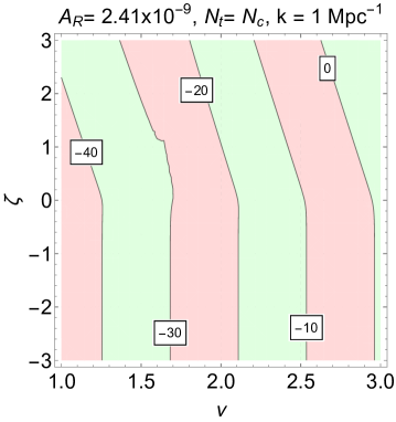
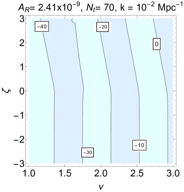
Figure 1: The parameter space is described in the $(\nu,\zeta)$ plane for two different values of the number of efolds and for two complementary comoving scales. The labels appearing on the various isospectral curves denote te common logarithm of $\sqrt{P_{B}(k,\tau_{c})}$ expressed in Gauss.

To investigate the role of the initial data we shall now define the protoinflationary boundary $\tau_{*}$ as the approximate moment at which the background starts inflating. We can then assume, without loss of generality, that $|b_{-}(k)|^{2}=(k/k_{*})^{\zeta}$ where $k_{*}\simeq\tau_{*}^{-1}$. The scale $k_{*}$ is, by definition, the maximal wavenumber of the initial spectrum. The energy density of the initial state at $\tau_{*}$ is approximately $d\rho_{*}\simeq 2|b_{-}(k)|^{2}d^{3}k/(2\pi)^{3}$. If $\zeta>-4$ the total energy density is is dominated by the largest scale (i.e. $\rho_{*}={\mathcal{O}}(k_{*}^{4})$). To avoid an excessive contribution of the initial energy density to the dynamics of the background we must require $8\pi\rho_{*}\ll 3H^{2}M_{P}^{2}$ implying

$$\frac{k}{k_{*}}=\frac{12.63}{Q_{i}}\,e^{-(N_{c}-N)}\,\biggl{(}\frac{k}{\mathrm{Mpc}^{-1}}\biggr{)}\,\biggl{(}\frac{h_{0}}{0.7}\biggr{)}^{-1}\,\biggl{(}\frac{{\mathcal{A}}_{{\mathcal{R}}}}{2.41\times 10^{-9}}\biggr{)}^{1/4}\biggl{(}\frac{\epsilon_{H}}{0.01}\biggr{)}^{1/4},$$ (28)

where $Q_{i}=H_{*}a_{*}/\sqrt{H_{i}M_{P}}<1$ if the energetic content of the initial state. In practice we can choose, for instance, $Q_{i}={\mathcal{O}}(10^{-4})$ as a reasonable fiducial value. Note that when the initial state is thermal $|b_{-}(k)|^{2}\to 1/(e^{k/k_{T}}-1)$ (as implied by the Bose-Einstein occupation number) where $k_{T}$ coincides, in the present units, with the putative comoving temperature of the initial state. This case will not be explicitly discussed here but it has been carefully scrutinized in Ref. [12].

The two-point function if the magnetic field intensity at coincident times is derived from Eq. (8) and it is

$$\langle\hat{B}_{i}(\tau_{c},\vec{x})\hat{B}_{i}(\tau_{c},\vec{x}+\vec{r})\rangle=2\int d\ln{k}\,P_{B}(k,\tau_{c})j_{0}(k\,r),\qquad j_{0}(kr)=\frac{\sin{k\,r}}{k\,r},$$ (29)

implying that $P_{B}(k,\tau_{c})$ and $\sqrt{P_{B}(k,\tau_{c})}$ measure, respectively, the energy density the field intensity over the typical wavenumber $1/r$. For the applications to magnetogenesis problems [10, 11] it is useful to compute the physical power spectrum expressed in units of Gauss (G, in what follows) and at the time of the gravitational collapse of the protogalaxy. The result of this calculation is

$$\frac{\sqrt{P_{b}(k,\tau_{c})}}{\mathrm{G}}=10^{-10.84}\,\biggl{(}\frac{{\mathcal{A}}_{{\mathcal{R}}}}{2.41\times 10^{-9}}\biggr{)}^{1/2}\,\biggl{(}\frac{\Omega_{\mathrm{R}0}}{4.15\times 10^{-5}}\biggr{)}^{1/2}\,\cos{\theta_{W}}{\mathcal{M}}(\nu,\zeta,k,k_{*}),$$ (30)

where, as already mentioned, $\sqrt{P_{B}(k,\tau)}=a^{2}(\tau)\chi(\tau)\sqrt{P_{b}(k,\tau)}$ for $\tau<\tau_{re}$ and $\sqrt{P_{B}(k,\tau)}=a^{2}(\tau)\sqrt{P_{b}(k,\tau)}$ for $\tau>\tau_{re}$; the function ${\mathcal{M}}(\nu,\zeta,k,k_{*})$ appearing in Eq. (30) is given by

$${\mathcal{M}}(\nu,\zeta,k,k_{*})=\biggl{(}\frac{k}{a_{i}H_{i}}\biggr{)}^{5/2-\nu}\biggl{\{}1+2\biggl{(}\frac{k}{k_{*}}\biggr{)}^{\zeta}+2\biggl{(}\frac{k}{k_{*}}\biggr{)}^{\zeta/2}\sqrt{1+\biggl{(}\frac{k}{k_{*}}\biggr{)}^{\zeta}}\cos{[2q(\nu)]}\biggr{\}}^{1/2}.$$ (31)

In Eq. (30) we used that the non-screened vector modes of the hypercharge field the project on the electromagnetic fields through the cosine of the Weinberg angle $\cos{\theta_{W}}$.

Equations (30) and (31) shall now be analyzed in the ($\nu$, $\zeta$) plane illustrated in Fig. 1 where we plot the isospectral lines (i.e. the lines of the parameter space over which the magnetic power spectrum is approximately constant) for few physically meaningful choices of the parameters. When $\zeta\to 0$ the scale-invariant limit of the magnetic power spectrum corresponds to $\nu\to 5/2=2.5$ with typical amplitude ${\mathcal{O}}(10^{-10})$G: this limit can be verified in both plots of Fig. 1. When $\zeta\neq 0$, quasi-flat power spectra can be obtained as long as $\nu$ remains in the region where $\log{[\sqrt{P_{B}(k,\tau_{c})}]}={\mathcal{O}}(-10)$. In the left plot of Fig. 1 we illustrated the benchmark scale of the gravitational collapse of the protogalaxy (i.e. $k={\mathcal{O}}(1)\,\mathrm{Mpc}^{-1}$) when the number of efolds is just critical (i.e. $N_{t}=N_{c}$); in the right plot we instead considered a larger typical length-scale (i.e. smaller wavenumber $k={\mathcal{O}}(10^{2})\,\mathrm{Mpc}^{-1}$) and a larger total number of efolds (i.e. $N_{t}=70>N_{c}$). What matters is the inclination of the (almost straight) isospectral lines for $\zeta>0$. Figure 1 shows that for $N_{t}>N_{c}$ the inclination diminishes and the lines become more and more vertical when $N_{t}\gg N_{c}$. The latter observation shows that as long as $N_{t}={\mathcal{O}}(N_{c})$ the parameter space of inflationary magnetogenesis is comparatively larger than in the case $\zeta=0$: we pass from a point (i.e. $\zeta=0$ and $\nu\simeq 2.5$) to a whole isospectral line in the $(\nu,\zeta)$ plane.

If $\sqrt{P_{b}(k_{c},\tau_{c})}$ is approximately larger than about $10^{-24}$ G (but still much smaller than ${\mathcal{O}}(10^{-10})$ G) the observed galactic field intensity can only be reached if the fields are amplified (for $\tau>\tau_{re}$) by the combined action of the gravitational collapse and of the galactic rotation. The latter effect may hopefully transform, under various conditions, the kinetic energy of the plasma into magnetic energy [11]. The most optimistic estimates for the required initial conditions are derived by assuming that every rotation of the galaxy would increase the magnetic field of one efold. The number of galactic rotations since the collapse of the protogalaxy can be between $30$ and $35$, leading approximately to a purported growth of 13 orders of magnitude. If the dynamo action is totally absent, the required field should be ${\mathcal{O}}(10^{-11})$ G. In this case, during the collapse of the protogalaxy, the magnetic field will increase by about $5$ orders of magnitude. In the literature it is sometimes practical to refer to some hypothetical seed field supposedly present at the time of the collapse of the protogalaxy. By definition ${\mathcal{B}}_{seed}=\sqrt{P_{b}(k_{c},\tau_{c})}$ where following the standard conventions [11] we took $k_{c}={\mathcal{O}}(1)\,\mathrm{Mpc}^{-1}$. From the above considerations we have therefore that

$${\mathcal{O}}(10^{-24})\,\mathrm{G}\leq{\mathcal{B}}_{seed}(\tau_{c})\leq{\mathcal{O}}(10^{-12})\mathrm{G}.$$ (32)

After the gauge modes reenter the effective horizon the approximate flux conservation implies ${\mathcal{B}}_{seed}(\tau_{c})={\mathcal{B}}_{seed}(\tau_{re})(H_{0}/M_{P})\sqrt{\Omega_{R0}/[\pi\epsilon_{H}{\mathcal{A}}_{{\mathcal{R}}}]}$ and Eq. (32), at $\tau_{re}$ can be written, up to the insignificant logarithmic corrections discussed above, as:

$${\mathcal{O}}(10^{33})\,\mathrm{G}\leq{\mathcal{B}}_{seed}(\tau_{re})\leq{\mathcal{O}}(10^{45})\mathrm{G}.$$ (33)

Equations (32) and (33) are insensitive to the properties of the initial state but they depend on the postinflationary thermal history, as already discussed in the past [12].

In summary the junction conditions for the gauge fields are compatible with sudden and delayed transitions of the effective horizon. The dynamical evolution of the gauge modes has been rephrased in terms of a pair of integral equations related by duality transformations. After showing how the continuity of the susceptibility and of its first derivative determines the hypermagnetic and hyperelectric power spectra, explicit examples of smooth transitions have been proposed to corroborate the analytic discussion. The general arguments based on the continuity of the effective horizon are valid up to logarithmic corrections which are numerically not significant when the gauge modes reenter the effective horizon. Moreover, after reentry these corrections are anyway overwhelmed by the dominance of the conductivity. As long as the total duration of the inflationary phase is nearly minimal the spectral slopes may be directly affected by the properties of the initial state. In the latter case case the parameter space of quasi-flat spectra gets larger. Conversely, when the number of efolds increases beyond a certain critical value, the present findings reproduce the previous results since the effects of the initial state are exponentially suppressed.

References

- [1] S. Weinberg, “Cosmology”, (Oxford, Oxford University Press, 2008).
- [2] S. Weinberg, Phys. Rev. D 67, 123504 (2003).
- [3] M. Giovannini, “A primer on the physics of the cosmic microwave background,” (World Scientific, Singapore, 2008).
- [4] M. Giovannini, Phys. Rev. D 88, no. 8, 083533 (2013); Phys. Rev. D 92, no. 4, 043521 (2015); Phys. Rev. D 92, no. 12, 121301 (2015); G. Tasinato, JCAP 1503, 040 (2015); R. Z. Ferreira and J. Ganc, JCAP 1504, no. 04, 029 (2015); M. Giovannini, Phys. Rev. D 93, no. 4, 043543 (2016).
- [5] G. Feinberg and J. Sucher, Phys. Rev. A 2, 2395 (1970); Phys. Rev. D 20, 1717 (1979).
- [6] S. Deser and C. Teitelboim, Phys. Rev. D 13, 1592 (1976); S. Deser, J. Phys. A 15, 1053 (1982); M. Giovannini, JCAP 1004, 003 (2010).
- [7] B. Ratra, Astrophys. J. Lett. 391, L1 (1992); M. Gasperini, M. Giovannini, and G. Veneziano, Phys. Rev. Lett. 75, 3796 (1995); M. Giovannini, Phys. Rev. D 56, 3198 (1997); M. Giovannini, Phys. Rev. D 64, 061301 (2001).
- [8] K. Bamba and M. Sasaki, JCAP 02, 030 (2007); K. Bamba JCAP 10, 015 (2007); M. Giovannini, Phys. Lett. B 659, 661 (2008).
- [9] K. Bamba, Phys. Rev. D 75 083516 (2007); J. Martin and J. ’i. Yokoyama, JCAP 0801, 025 (2008); M. Giovannini, Lect. Notes Phys. 737, 863 (2008); S. Kanno, J. Soda and M. -a. Watanabe, JCAP 0912, 009 (2009); K. Bamba, Phys. Rev. D 91, 043509 (2015); K. W. Ng, S. L. Cheng and W. Lee, Chin. J. Phys. 53, 110105 (2015); P. Qian, Y. F. Cai, D. A. Easson and Z. K. Guo, Phys. Rev. D 94, no. 8, 083524 (2016); R. Koley and S. Samtani, JCAP 1704, no. 04, 030 (2017); M. Giovannini, Phys. Lett. B 771, 482 (2017).
- [10] M. Giovannini, Phys. Rev. D 95, no. 8, 083501 (2017); M. Herranen, T. Markkanen, S. Nurmi, and A. Rajantie, Phys. Rev. Lett. 115, 241301 (2015); K. Enqvist, T. Meriniemi, and S. Nurmi, J. Cosmol. Astropart. Phys. 10, 057 (2013); 07 025 (2014); M. Giovannini and M. E. Shaposhnikov, Phys. Rev. D 62, 103512 (2000).
- [11] C. Heiles, Annu. Rev. Astron. Astrophys. 14, 1 (1976); P.P. Kronberg, Rep. Prog. Phys. 57, 325 (1994); K. Enqvist, Int. J. Mod. Phys. D 07, 331 (1998); C.L. Carilli and G.E. Taylor, Ann. Rev. Astron. Astrophys. 40, 319 (2002); M. Giovannini, Int. J. Mod. Phys. D 13, 391 (2004).
- [12] M. Giovannini, Phys. Rev. D 86, 103009 (2012); Phys. Rev. D 85, 101301 (2012).