Can the symmetry breaking in the SM
be determined by the Top-Higgs Yukawa interaction?

Abstract

In this letter, we first resume the results of a previous article (EPJC(2011)71:1620). That work considered a simple model of QCD including a Yukawa interaction with a scalar field. Its two loop effective potential for the scalar field, predicted a 126 GeV Higgs mass after the minimum of the potential was fixed at a mean scalar field giving a 175 GeV Top quark mass. However, a high value of the strong coupling was required ($\alpha=\frac{g^{2}}{4\pi}$ close to 1) to get these values. After reviewing the results of this study, an idea for extending the work is simply advanced here: to consider the running strong coupling, in order to decide whether or not, the usual values of the strong interactions have the chance of justifying the experimentally known values of the Higgs and Top quark masses. It is underlined that a positive result of the proposed task will suggests the possibility of basing the SM breaking of symmetry, on the so called second minimum of this model. This could also identify the essential role of QCD in this effect. Results of the further examination of this question will be presented elsewhere.

In ref. cabo a simple massless QCD model including only one quark type and a singlet scalar field with a Yukawa interaction between them, was investigated. The aim of the study was to explore a suspicion about that the so called ”second minimum” of the Standard Model (SM) could in fact be responsible for the symmetry breaking in the SM. As it is known, this minimum, in addition to the usual one exhibited by the Higgs potential, is the result of the Yukawa interaction of the Higgs field with the Top quark second-1 ; second-2 ; second-3 . This idea emerged after noting that this new minimum got its relevance only after the SM calculations arrived up to the two loop level. Then, the question emerges about what could be the result of an attempt to construct the SM around this new radiative corrections determined minimum. Up to our knowledge, there had not been attempts to answer this question in the past literature. These are the main motivations in considering the study in the work in reference cabo . The results of that work were inconclusive, in spite of the fact the correct experimental values of the Higgs and the Top quark masses were able to be fixed by choosing a definite value of the strong coupling parameter. It happened, that the value of this parameter was a high one: $\frac{g^{2}}{4\pi}$ close to $1$. In this letter we start by reviewing the results in cabo for afterwards simply propose an idea which could perhaps justify to further study the possibility of basing the SM in the so called ”second minimum”.

Let us now start reviewing the main elements of the model discussed in cabo . The generating functional of the model is based in an action including a simple singlet scalar field interacting with only one type of quark. The functional was chosen in the form

$$Z[j,\eta,\overline{\eta},\xi,\overline{\xi},\rho]=\frac{1}{\mathcal{N}}\int\mathcal{D}[A,\overline{\Psi},\Psi,\overline{c},c,\phi]\exp[i\text{ }S[A,\overline{\Psi},\Psi,\overline{c},c,\phi]],$$ (1)

The action was taken in the form written below, in which in addition to the usual massless QCD action, it was only considered a quark field Yukawa interacting with a scalar field. To simplify the discussion, the free action of the scalar field was defined as a massless free term in the absence of self-interaction. The various terms in the action, after decomposed in free and interaction parts, are written below

$$S =\int dx(\mathcal{L}_{0}\mathcal{+L}_{1}\mathcal{)},$$ (2)

$$\mathcal{L}_{0} =\mathcal{L}^{g}+\mathcal{L}^{gh}+\mathcal{L}^{q}+\mathcal{L}^{\phi},$$ (3)

$$\mathcal{L}^{g} =-\frac{1}{4}(\partial_{\mu}A_{\nu}^{a}-\partial_{\nu}A_{\mu}^{a})(\partial^{\mu}A^{a,\nu}-\partial^{\nu}A^{a,\mu})-\frac{1}{2\alpha}(\partial_{\mu}A^{\mu,a})(\partial^{\nu}A_{\nu}^{a}),$$ (4)

$$\mathcal{L}^{gh} =(\partial^{\mu}\chi^{\ast a})\partial_{\mu}\chi^{a},$$ (5)

$$\mathcal{L}^{q} =\overline{\Psi}(i\gamma^{\mu}\partial_{\mu})\Psi,$$ (6)

$$\mathcal{L}^{\phi} =\partial^{\mu}\phi\partial_{\mu}\phi,$$ (7)

$$\mathcal{L}_{1} =-\frac{g}{2}f^{abc}(\partial_{\mu}A_{\nu}^{a}-\partial_{\nu}A_{\mu}^{a})A^{b,\mu}A^{c,\nu}-g^{2}f^{abe}f^{cde}A_{\mu}^{a}A_{\nu}^{b}A^{c,\mu}A^{d,\nu}-$$

$$-gf^{abc}(\partial^{\mu}\chi^{\ast a})\chi^{b}A_{\mu}^{c}+g\overline{\Psi}T^{a}\gamma^{\mu}\Psi A_{\mu}^{a}+\overline{\Psi}\Psi\phi.$$ (8)

After constructing the Feynman expansion being associated to the above generating function and classical action, the evaluation of the effective potential as a function of an homogeneous scalar (Higgs resembling) field was considered in reference cabo , up to the two loop approximation. The one loop term of the potential as a function of the scalar field $\phi$ was defined by the quark one loop diagram with the mean scalar field as a background. It took the form:

$$\Gamma^{(1)}[\phi] =-V^{(D)}N\int\frac{dp^{D}}{i\text{ }(2\pi)^{D}}Log[Det\text{ }(G_{ii^{\prime}}^{(0)rr^{\prime}}(\phi,p))],$$ (9)

$$D =4-2\epsilon.$$

This contribution is illustrated in figure 1.

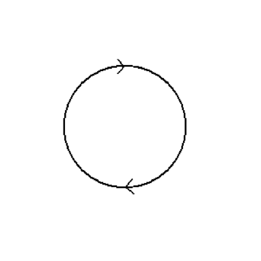
Figure 1: The figure shows the quark one loop correction. The result depends on the scalar ”mass” field $\phi$ through the quark free propagator which is the usual free Green function of QCD, in which the mass is substituted by $\phi$.

After evaluating the color and spinor traces and integrating in dimensional regularization the effective action density took the form

$$\gamma^{(1)}[\phi]=\frac{\Gamma^{(1)}[\phi]}{\frac{V(D)}{\mu^{2\epsilon}}}=\frac{2N\text{ }\Gamma(\epsilon-1)}{(\frac{D}{2})(4\pi)^{2-\epsilon}}\phi^{2}(\frac{\phi}{\mu})^{-2\epsilon}.$$ (10)

Next, by subtracting the pole in $\epsilon$ in order to employ the MS substraction scheme, passing to the limit $D=4-2\epsilon\rightarrow$ 4 and changing the sign, gave the Higgs potential one loop contribution in the form

$$v^{(1)}[\phi]=-\frac{3\phi^{4}}{8\pi^{2}}(-3+2\gamma+2Log(\frac{\phi^{2}}{2\pi\mu^{2}})).$$ (11)

Note the important fact that the one loop potential for the scalar field determined by the quark loop, is unbounded from below.

The two loop contribution associated to the quark gluon interaction in the background of the scalar Higgs field in reference cabo is illustrated in figure 2.

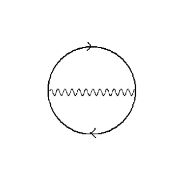
Figure 2: The two loop term determined by the strong interaction. Again the $\phi$ dependence of the result is introduced though the free quark propagator.

By writing the diagram expression and calculating the color and spinor traces, this term was written in the form

$$\Gamma^{(2)}[\phi]=-V^{(D)}g^{2}(N^{2}-1)\int\frac{dp^{D}dq^{D}}{i^{2}\text{ }(2\pi)^{2D}}\frac{D\phi^{2}-(D-2)p.(p+q)}{q^{2}(p^{2}-\phi^{2})((p+q)^{2}-\phi^{2})}.$$ (12)

The integrals appearing were integrated by employing the results in fleischer . After dividing by the volume the total action density, associated to this two loop contribution, decomposes in the following two dimensionally regularized terms:

$$\gamma^{(2,1)}[\phi] =\frac{\Gamma^{(2,1)}[\phi]}{\frac{V(D)}{\mu^{2\epsilon}}}=-v^{(2,1)}[\phi]$$

$$=-\frac{2g_{0}^{2}(N^{2}-1)}{\text{ }(2\pi)^{2D}}\frac{A(\epsilon)\pi^{4-2\epsilon}}{\epsilon^{2}}\phi^{4}(\frac{\phi^{2}}{\mu^{2}})^{-2\epsilon}\ \ \ \ \ \ \ \ \ \$$ (13)

and

$$\gamma^{(2,2)}[\phi] =\frac{\Gamma^{(2,2)}[\phi]}{\frac{V(D)}{\mu^{2\epsilon}}}=-v^{(2,2)}[\phi]$$

$$=V^{(D)}\frac{g_{0}^{2}\mu^{2\epsilon}(N^{2}-1)2(1-\epsilon)}{\text{ }2(2\pi)^{8-4\epsilon}}\pi^{4-2\epsilon}(\Gamma(\epsilon-1))^{2}\phi^{4}(\phi^{2})^{-2\epsilon}.$$ (14)

Further, by minimally subtracting the poles of these expressions, taking the limit $\epsilon\rightarrow 0$ and numerically evaluating all the constants for getting a simpler expression, the potential density (the negative of the action density) associated to this two loop contribution becomes

$$v^{(2)}[\phi] =5.34687\times 10^{-5}\phi^{4}{\LARGE(}1227.16+474.276\text{ }g_{0}^{2}-$$

$$12.0(\text{ }29.6088+13.5253\text{ }g_{0}^{2})\text{ }Log(\frac{\phi^{2}}{\mu^{2}})+$$

$$12.0\text{ }g_{0}^{2}\text{ }(Log(\frac{\phi^{2}}{\mu^{2}}))^{2}{\LARGE).}$$ (15)

In this expression, the leading logarithm term in the scalar field is squared and has a positive coefficient, making the result bounded from below.

Finally, in reference cabo it was considered the two loop contribution associated with the interaction of the radiation scalar field with the quarks which diagram is shown in figure 3.

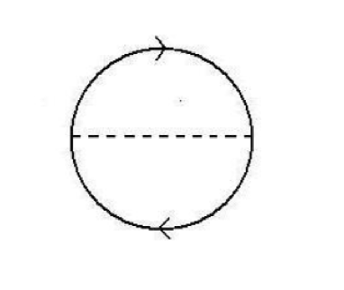
Figure 3: The diagram corresponding to the radiative corrections of the ”mass” field $\phi$ in the two loop order.

It followed that the analytic form of the Feynman diagram became very similar to the previous one

$$\Gamma_{Y}^{(2)}[\phi]=V^{(D)}2N\int\frac{dp^{D}dq^{D}}{i^{2}\text{ }(2\pi)^{2D}}\frac{p^{2}-\frac{q^{2}}{4}+\phi^{2}}{q^{2}((p+\frac{q}{2})^{2}-\phi^{2})((p-\frac{q}{2})^{2}-\phi^{2})},$$ (16)

and it was calculated also in a close manner to find for the action density and potential associated to this term

$$\gamma_{Y}^{(2)}[\phi] =-v_{Y}^{(2)}[\phi]$$

$$=\frac{4N}{\text{ }(2\pi)^{8-4\epsilon}}\frac{A(\epsilon)\pi^{4-2\epsilon}}{\epsilon^{2}}\phi^{4}(\frac{\phi^{2}}{\mu^{2}})^{-2\epsilon}$$

$$-\frac{N}{\text{ }(2\pi)^{8-4\epsilon}}\pi^{4-2\epsilon}(\Gamma(\epsilon-1))^{2}\phi^{4}(\frac{\phi^{2}}{\mu^{2}})^{-2\epsilon}.$$ (17)

Subtracting the divergent terms in the Laurent expansion with respect to the parameter $\epsilon$, gave the following finite contribution.

$$v_{Y}^{(2)}[\phi]=-0.0000601522\text{ }m^{4}\left(332.744-123.833Log[\frac{m^{2}}{\mu^{2}}]+12.0\,Log[\frac{m^{2}}{\mu^{2}}]^{2}\right).$$ (18)

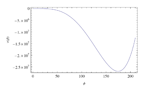
Figure 4: The effective potential for the ”mass” field $\phi$ for the value of the scale $\mu$ determining that the value of $\phi$ taken at the minimum potential, is approximately equal to the top quark mass $m_{top}~{}175\,\,GeV$.

Then, in reference cabo , it was further considered the study of the potential and its minimum as a function of the parameters. Specifically, the coupling and renormalization scale parameter $\mu$ were chosen as satisfying the one loop RG expression.

$$g_{0}(\mu,\Lambda_{QCD})=2\sqrt{\frac{2}{7}}\pi\sqrt{\frac{1}{Log(\frac{\mu}{\Lambda_{QCD}})}},$$ (19)

and the value $\Lambda_{QCD}$ = 217 MeV was selected. Next, $\mu$ was changed up to fix the mean scalar field $\phi$ to a value determining the top quark mass: 174.599 GeV. The resulting curve for the scalar field potential is shown in figure 4. An interesting conclusion implied by this plot was that the second derivative at the potential minimum is $m_{\phi}=126.76\,\,GeV$, which is close to the recently measured value of the Higgs mass. At the year 2011 in which the paper cabo appeared, the Higgs mass was still unknown. However, at that time the mass value $114$ $GeV$, indicated by some low statistic data measured at ALEPH experiment at CERN, led to suspect the link of the result with the Higgs mass. However, it is needed to remark that in the simplified model considered in cabo , the scale $\mu$ , which allowed the top mass fixation lies within the non perturbative infrared region: $\mu=0.498\,\,GeV$, which determines a coupling value $\alpha=\frac{g_{0}^{2}}{4\pi}=1.077$. Therefore, the result about the possibility of basing the SM in the ”second minimum” remained inconclusive at that time. Therefore, the possibility of fixing the observed value of the top mass in the scheme, and with it, the $126.76\,\,GeV$ estimation of the Higgs particle mass remained open.

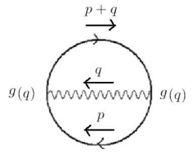
Figure 5: The two loop contribution depending on the momentum dependent running coupling.

The proposal

As it was mentioned, a main objective of the present letter, in addition to reviewing the ideas of the paper cabo , is to identify and advance a possibility for the normal strength of the strong coupling to becomes able in justifying the physical values for the Top and Higgs masses in the SM. As it was mentioned, the central limitation of the results discussed in reference cabo , was the fact that a slightly high value of strong coupling was required to fix the Top and Higgs masses. The coupling values employed for the evaluations were assumed as constants. Therefore, the idea comes to the mind about that the running with momenta strong coupling should increase at low momenta. Henceforth, the possibility appears that using a momenta dependent coupling in the two loop evaluation of the closed fermion loop contracted with the gluon propagator, could furnish similar results for the Higgs potential that the ones obtained for the relatively high constant coupling employed in reference cabo . The two loop contribution associated to the quark gluon interaction in the background of the scalar field, but including a transferred gluon momentum $q$ dependence of the strong coupling is shown in figure 5. The calculation of the expression in which the coupling is running becomes more involved, since the evaluations of the two loop integrals should be done numerically due to the momentum dependence of the $g(p)$. It is clear that the first integration over the momentum $p$ can be done, but it will include one loop infinities. Thus the best way of proceeding seems to be first constructing the renormalized form of the model, for further evaluating the finite part of the diagram under consideration. Afterwards, the best form of inputting the running coupling should more easily discussed.

The investigation of this question will be considered elsewhere. If the conclusions become positive ones, the measured Top and Higgs masses might be defined by a symmetry breaking based in the second minimum of the Higgs potential, in place than on the Higgs classical minimum.

- (1) A. Cabo, Eur. Phys. J. C (2011) 71:1620
- (2) M. Gonderinger, Y. Li, H. Patel, M. Ramsey-Musolf, J. High Energy Phys. 1001, 053 (2010)
- (3) 21. J.A. Casas, J.R. Espinosa, M. Quiros, Phys. Lett. B 382, 374 (1996)
- (4) C.D. Froggatt, H.B. Nielsen, Phys. Lett. B 368, 96 (1996)
- (5) J. Fleischer and O. V. Tarasov, Z. Phys. C 64, 413 (1994)