Extreme-scale motions in turbulent plane Couette flows

Abstract

We study the large-scale motions in turbulent plane Couette flows at moderate friction Reynolds number up to $Re_{\tau}=500$. Direct numerical simulation domains were as large as $100\pi\delta\times 2\delta\times 5\pi\delta$, where $\delta$ is half the distance between the walls. The results indicate that there are streamwise vortices filling the space between the walls that remain correlated over distances in the streamwise direction that increase strongly with the Reynolds number, so that for the largest Reynolds number studied here, they are correlated across the entire $100\pi\delta$ length of the domain. The presence of these very long structures is apparent in the spectra of all three velocity components and the Reynolds stress. In DNS using a smaller domain, the large structures are constrained, eliminating the streamwise variations present in the larger domain. Near the center of the domain, these large scale structures contribute as much as half of the Reynolds shear stress.

1 Introduction

Planar Couette and Poiseuille flows are the simplest canonical configurations for the computational study of wall-bounded turbulence. Since Kim et al. (1987) carried out direct numerical simulation (DNS) of Poiseuille flows at $Re_{\tau}=180$, DNS has been widely used to study the physics of wall-bounded turbulence at Reynolds numbers ($Re$) up to $Re_{\tau}=5200$ (Moser et al., 1999; del Álamo et al., 2004; Hoyas & Jiménez, 2006; Lozano-Durán & Jiménez, 2014; Bernardini et al., 2014; Lee & Moser, 2015). Even higher $Re$ flows have been studied experimentally in pipes at $Re_{\tau}=10^{5}$ (Hultmark et al., 2012) and zero-pressure-gradient (ZPG) boundary layers at $Re_{\tau}=6.5\times 10^{5}$ (Marusic et al., 2010).

On the other hand, the study of planar Couette flow has been more limited in number of studies and Reynolds number, both experimentally and computationally. One of the reasons is the existence of very large-scale motions in Couette flow that are particularly challenging to represent in DNS. The first DNS study of turbulent Couette flows was at $Re_{\tau}=170$ by Lee & Kim (1991). They used a periodic computational domain size of $4\pi\delta\times 8/3\pi\delta$ in the streamwise and spanwise directions, respectively, where $\delta$ is half the distance between the walls. In their simulation, the most energetic motion at the center of the domain is at wavenumbers $k_{x}\delta=0$ and $k_{z}\delta=1.5$ which has no variation in the streamwise direction and is clearly an artifact of the finite simulation domain size. Komminaho et al. (1996) also performed DNS at $Re_{\tau}=52$ with a simulation domain of $28\pi\delta\times 8\pi\delta$ and obtained energy spectra with DNS peaks at the same wavenumbers. Later, Tsukahara et al. (2006); Avsarkisov et al. (2014); Pirozzoli et al. (2014) performed DNS at Reynolds numbers up to $Re_{\tau}=126$ ($64\delta\times 6\delta$), $Re_{\tau}=550$ ($20\pi\delta\times 6\pi\delta$) and $Re_{\tau}=986$ ($18\pi\delta\times 8\pi\delta$), respectively. Their results show that the wavelength of large-scale motion is approximately $\lambda_{z}=5\delta$. However, the domain sizes for the previous works were not long enough to determine the extent of the large-scale motion. On the other hand, the experimental study with moving belts by Kitoh & Umeki (2008); Kitoh et al. (2005) at $Re_{\tau}=192$ shows that the extent of the large-scale motion in the streamwise direction is $\lambda_{x}\approx 40\delta-60\delta$.

Large-scale motions in transition in planar Couette flows have also been observed. For example, Tillmark & Alfredsson (1992) performed moving belt experiments with an aspect ratio $L_{x}/\delta=150$ and observed growing turbulent spots with the streamwise extent of about $60\delta$. Using a moving belt facility with aspect ration 385, Prigent et al. (2003) observed spots with streamwise coherence over approximately $250\delta$. More recently, using particle image velocimetry (PIV) in an aspect ration 100 belt experiment, Couliou & Monchaux (2015) studied growth of large-scale motions. Finally, using DNS, Duguet et al. (2010) studied the formation of turbulent spots with $800\delta$ long simulation domains.

The goal of the current study is to study the very large-scale motions in Couette flow by simulating them in computational domains large enough to allow their streamwise extent to be determined. Through the discussion, similarity to and contrasts with turbulent Poiseuille flow will also be made through reference to the DNS study by Lee & Moser (2015) and Lozano-Durán & Jiménez (2014). When comparing dissimilar flows, there is always ambiguity as to how to consistently compare Reynolds numbers. Here the Reynolds number $Re_{\tau}$ is defined based on friction velocity and the domain half-width $\delta$, as is common in Poiseuille flow. However, in a study of transitional flows, Barkley & Tuckerman (2007) suggest that the appropriate length scale in Couette flow is the full width, since the shear does not change sign across the layer. Assessing appropriate length scales for comparison to Poiseuille flow would require Couette flow simulations at much higher Reynolds number than reported here, which is out of scope for the current study. For our purposes, it is sufficient to note that the Couette flows studied here could be comparable to Poiseuille flows with Reynolds number equal to or up to twice as high as the Couette Reynolds number. In the remainder of this paper, we present details of the current simulations (§2) followed by simulation results (§3). Finally, we provide concluding remarks in §4.

2 Numerical Simulations

In the discussion to follow, $x$, $y$ and $z$ denote the streamwise, wall-normal and spanwise directions, respectively, and the corresponding velocity components are denoted as $u$, $v$, and $w$, respectively. Angle brackets $\langle\psi\rangle$ indicate the expected value or average of the quantity $\psi$ over $x$ and $z$ directions and time, $t$. In addition, quantities with prime denote the fluctuation from the average, i.e. $\psi^{\prime}=\psi-\langle\psi\rangle$ and $\langle\psi^{\prime}\rangle=0$.

We performed direct numerical simulations of incompressible turbulent Couette flow by solving the Navier-Stokes equations using the velocity-vorticity formulation introduced by Kim et al. (1987). The flow is driven by two parallel planes moving in opposite directions at constant speed, and there is no mean pressure gradient. We specify a finite rectangular simulation domain of size $L_{x}\times L_{z}$ with periodic boundary conditions in the wall-parallel ($x$ and $z$) directions. Boundary conditions at the walls are no-slip and no-penetration. A Fourier-Galerkin discretization with $N_{x}\times N_{z}$ Fourier modes is used in the wall-parallel directions, with effective resolution defined by the Nyquist grid spacing $\Delta x=L_{x}/N_{x}$ and $\Delta z=L_{z}/N_{z}$. In the wall-normal ($y$) direction, we use a seventh order basis spline (B-spline) collocation method, with knots defined by:

$$y_{i,\mathrm{knot}}=\delta\sin\left(\frac{i\pi}{N_{y}-7}-\frac{\pi}{2}\right),\quad i=0,1,2,\cdots(N_{y}-7)$$ (1)

where $N_{y}$ is the number of B-splines in the representation and the number of collocation points. Note that the knots near the walls are denser than knots at the center of domain. The collocation points are defined as the Greville abscissae (Johnson, 2005). See Lee et al. (2013, 2014); Lee & Moser (2015) for more information about the numerical method.

Case	$Re_{\tau}$	$L_{x}/\delta$	$L_{z}/\delta$	$N_{x}$	$N_{y}$	$N_{z}$	$\Delta x^{+}$	$\Delta y^{+}_{w}$	$\Delta y^{+}_{c}$	$\Delta z^{+}$	$Tu_{\tau}/\delta$	Reference
R93S	092.93	020$\pi$	5$\pi$	00640	128	0288	09.12	0.031	2.41	5.07	197.94	Current
R93L	092.91	100$\pi$	5$\pi$	03072	128	0288	09.50	0.031	2.41	5.06	185.83	Current
R220S	219.15	020$\pi$	5$\pi$	01280	192	0768	10.76	0.032	3.72	4.48	187.16	Current
R220L	219.48	100$\pi$	5$\pi$	06144	192	0768	11.22	0.032	3.73	4.49	164.61	Current
R500S	502.63	020$\pi$	5$\pi$	03072	256	1536	10.28	0.040	6.34	5.14	150.79	Current
R500L	501.37	100$\pi$	5$\pi$	15360	256	1536	10.25	0.040	6.33	5.13	150.79	Current
R125A	131.60	020$\pi$	6$\pi$	00576	151	0384	14.36	0.746	2.14	6.46	027.10	Avsarkisov et al. (2014)
R180A	177.29	020$\pi$	6$\pi$	00864	251	0512	12.89	0.297	1.88	6.53	034.00	Avsarkisov et al. (2014)
R250A	243.74	020$\pi$	6$\pi$	01536	251	0768	09.97	0.408	2.59	5.98	053.00	Avsarkisov et al. (2014)
R550A	553.43	020$\pi$	6$\pi$	02592	251	1536	13.42	0.926	5.88	6.79	057.00	Avsarkisov et al. (2014)
R550P	546.75	060$\pi$	6$\pi$	08192	257	2048	12.58	0.041	6.71	5.03	005.00	Lozano-Durán & Jiménez (2014)

Table 1: Summary of simulation parameters. $N_{x}$ and $N_{z}$ are the number of Fourier modes, and $N_{y}$ is the number of collocation points. $\Delta y_{w}$ and $\Delta y_{c}$ of current work are the knot spacings at the wall and center line, respectively whereas $\Delta y_{w}$ and $\Delta y_{c}$ of works by Avsarkisov et al. (2014) and Lozano-Durán & Jiménez (2014) are the collocation point spacing. $Re_{\tau}=u_{\tau}\delta/\nu$ is the friction Reynolds number, and $Tu_{\tau}/\delta$ is the scaled total averaging time.

We simulated six cases with three different Reynolds numbers, $Re_{\delta}=U_{w}\delta/\nu$ where $U_{w}$ and $\nu$ are wall-speed and kinematic viscosity, respectively. The domain size in the streamwise direction was either $L_{x}=100\pi\delta$ or $20\pi\delta$, while the domain size in the spanwise direction was $L_{z}=5\pi\delta$ for all cases. We use $L_{x}=20\pi\delta$ for the small domain cases because this is the largest streamwise length used in previous DNS studies (Avsarkisov et al., 2014). In the spanwise direction, $L_{z}=5\pi\delta$ is smaller than the domain size used by Pirozzoli et al. (2014) ($L_{z}=8\pi\delta$), but it has been found to be sufficient to capture the large scale motions in the spanwise directions, as will be discussed in the next section. The resolution ($\Delta x^{+}$, $\Delta y^{+}$ and $\Delta z^{+}$) was chosen to be sufficient to represent the smallest dissipative motions, based on experience in other wall-bounded turbulent flows (see e.g. Lee & Moser, 2015). Table 1 catalogs the parameters defining the cases discussed here. The friction Reynolds number, $Re_{\tau}$, is based on the friction velocity, $u_{\tau}=\sqrt{\tau_{w}/\rho}$, where $\tau_{w}$ is the mean shear stress at the wall and $\rho$ is the fluid density. As is common in wall-bounded turbulence, a superscript $+$ designates a quantity normalized in wall units (i.e. normalized by $u_{\tau}$ and $\nu$).

Conservation of mean momentum requires that in stationary turbulent Couette flow, the total stress, which is the sum of the Reynolds and viscous shear stresses is a constant independent of $y$; particularly:

$$\tau_{\mathrm{total}}^{+}=\left\langle\frac{\partial u}{\partial y}\right\rangle^{+}-\langle u^{\prime}v^{\prime}\rangle^{+}=1$$ (2)

To ensure that the simulation results were statistically stationary, the total stress was monitored for consistency with (2). In all the simulation results presented here, the deviation from this analytic result was less than 0.2%, and less than the estimated sampling uncertainty determined by the technique outlined in Oliver et al. (2014). Estimated uncertainties in one-point statistics are included in Appendix A. In the following, we include data from Avsarkisov et al. (2014) for comparison, when possible.

3 Results

The mean velocity profiles for each Couette flow case are shown in figure 1. Both the mean velocity and the log-layer diagnostic $\beta=y^{+}\langle\partial u^{+}/\partial y^{+}\rangle$ are shown. As expected, the Reynolds numbers are too low to produce a convincing log-layer (constant $\beta$). Indeed in Poiseuille flow, an unambiguous log layer does not appear until $Re_{\tau}\approx 5000$ (Lee & Moser, 2015). Nonetheless, $\beta$ is more sensitive to small variations in the mean profile, and therefore it is a good diagnostic for detecting such differences. The $\beta$ profiles are consistent among all the cases up to $y^{+}\approx 50$. Beyond this, $\beta$ develops a plateau as $Re$ increases. However, at $Re_{\tau}\approx 500$, $\beta$ increases slowly until $y/\delta\approx 0.3$ then decreases sharply, as previously observed by (Avsarkisov et al., 2014; Orlandi et al., 2015). At the low Reynolds numbers, there is no discernible difference in $\beta$ between the small and large domain cases, but there is a non-negligible difference away from the wall in the R500 cases. In all cases, $\beta$ rolls up at the center, even in the higher Reynolds number cases in which it drops sharply above $y/\delta\approx 0.3$. This is required since at the center $d\beta/dy=\langle\partial u/\partial y\rangle>0$ because $\langle\partial^{2}u/\partial y^{2}\rangle=0$ by symmetry.

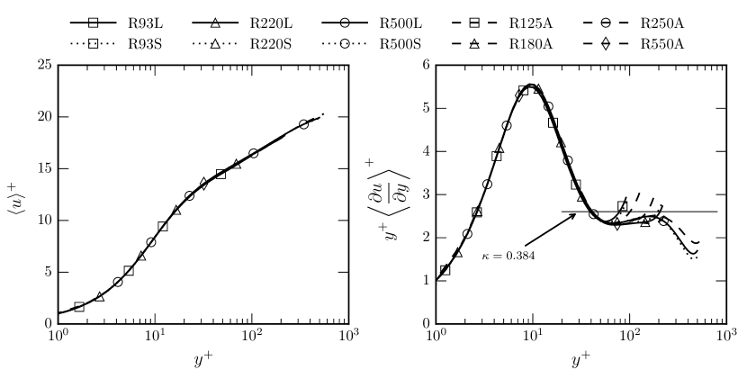
Figure 1: Mean velocity profile (left) and log-layer diagnostic function (right); Cases are defined in table 1.

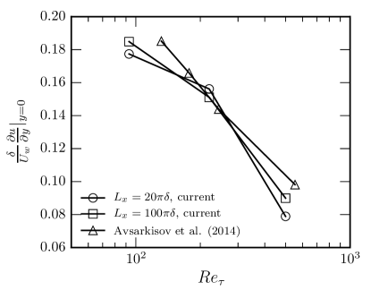
Figure 2: Mean velocity gradient at the center of channel

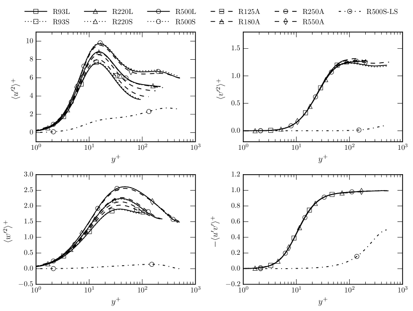
Figure 3: Profiles of the non-zero Reynolds stress components. Cases are defined in table 1, and the R500S-LS curves are the contribution of large-scale structures to the Reynolds stress.

The derivative of the mean velocity in the center of the domain is always zero in Poiseuille flows by symmetry. But in Couette flow the mean velocity is anti-symmetric, and so the velocity gradient is not necessarily zero at the center line, and therefore, neither is the production of turbulent kinetic energy. The behavior of the mean velocity gradient at the center as $Re$ increases is important to understanding the production in the outer region, but as noted by Avsarkisov et al. (2014) this remains controversial (Busse, 1970; Lund & Bush, 1980). Standard defect law scaling with $u_{\tau}$ and $\delta$, and the common assumption that $C_{f}=2u^{2}_{\tau}/U^{2}_{w}$ goes to zero as $Re\rightarrow\infty$ suggest that the mean velocity gradient scaled by $U_{w}$ and $\delta$ should go to zero at large Reynolds number. Indeed the data shown in figure 2 indicate that the gradient drops by almost a factor of 3 over the factor of 5 increase in Reynolds number investigated here. However, the Reynolds numbers are too low and the range of Reynolds numbers too small to suggest the high Reynolds number asymptotic behavior of the centerline derivative. It is also clear that there are modest differences in this derivative between the small and large domain cases, as large as 14% in the R500 case. Further, there are differences in the center line gradient between the current simulations and those of Avsarkisov et al. (2014), for unknown reasons. But this could be due to large uncertainties in the statistics at the center of channel.

The non-zero Reynolds stress components appear in Figure 3. When plotted in wall units, many features are similar to those in Poiseuille flow, especially near the wall, such as the increase in the peak of $u^{\prime 2}$ and to a lesser extent $w^{\prime 2}$ with Reynolds number. Away from the wall, particularly at the centerline, $u^{\prime 2}$ has a strong dependence on $Re$, which does not occur in Poiseuille flow (Lee & Moser, 2015). This may be related to the fact that the production of $u^{\prime 2}$ is zero in Poiseuille flow by symmetry, but not Couette flow. Note that there is a mild secondary peak in $u^{\prime 2}$ at approximately $y^{+}=200$ in the R500 cases. Such an outer peak does not occur in Poiseuille flow for $Re_{\tau}$ up to 5200 (Lee & Moser, 2015), but it is observed in both experiments at very high $Re$ in boundary layers and pipes (Hultmark et al., 2012; Marusic et al., 2010). There is no appreciable Reynolds number effect on $v^{\prime 2}$ or $u^{\prime}v^{\prime}$ in these flows, which is also different from Poiseuille flow. The effect of domain size on the Reynolds stress components is negligible in most cases. The one exception is $u^{\prime 2}$, in which there is a modest difference between the large and small domain cases away from the wall. In general, the current Reynolds stress component data agree with that from Avsarkisov et al. (2014), with only minor discrepancies, which are within the uncertainties described in Appendix A.

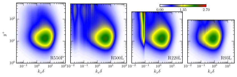
(a) $k_{x}\delta E_{uu}/u_{\tau}^{2}$

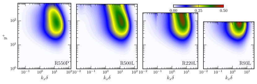
(b) $k_{x}\delta E_{vv}/u_{\tau}^{2}$

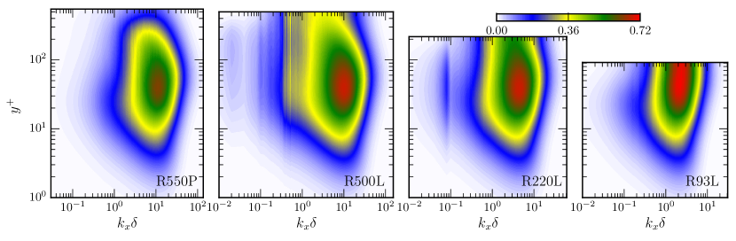
(c) $k_{x}\delta E_{ww}/u_{\tau}^{2}$

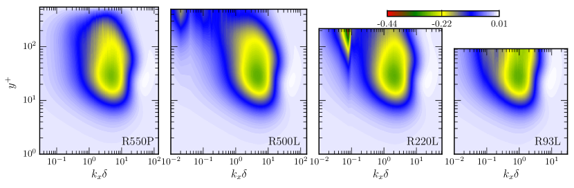
(d) $k_{x}\delta E_{uv}/u_{\tau}^{2}$

Figure 4: (Colour online) Contours of the $k_{x}$-premultiplied streamwise one-dimensional spectra of $u_{i}^{\prime}u_{j}^{\prime}$ for the long domain Couette flow cases identified in table 1, and the planar Poiseuille flow of Lozano-Durán & Jiménez (2014) at $Re_{\tau}=550$, labeled R550P.

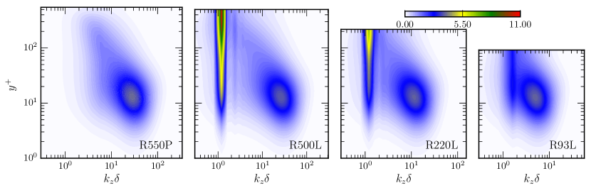
(a) $k_{z}\delta E_{uu}/u_{\tau}^{2}$

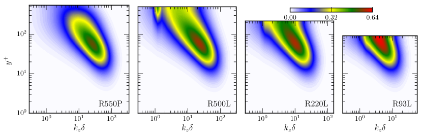
(b) $k_{z}\delta E_{vv}/u_{\tau}^{2}$

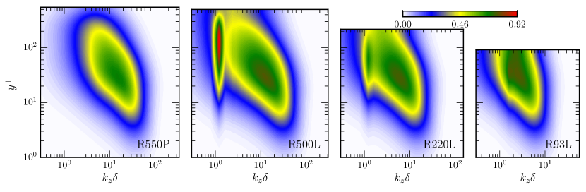
(c) $k_{z}\delta E_{ww}/u_{\tau}^{2}$

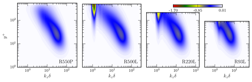
(d) $k_{z}\delta E_{uv}/u_{\tau}^{2}$

Figure 5: (Colour online) Contours of the $k_{z}$-premultiplied spanwise one-dimensional spectra of $u_{i}^{\prime}u_{j}^{\prime}$ for the long domain Couette flow cases identified in table 1, and the planar Poiseuille flow of Lozano-Durán & Jiménez (2014) at $Re_{\tau}=550$, labeled R550P.

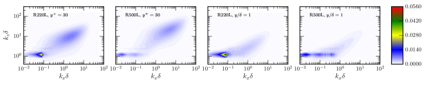
(a) $k_{x}k_{z}\delta^{2}E_{uu}/u_{\tau}^{2}$

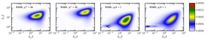
(b) $k_{x}k_{z}\delta^{2}E_{vv}/u_{\tau}^{2}$

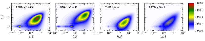
(c) $k_{x}k_{z}\delta^{2}E_{ww}/u_{\tau}^{2}$

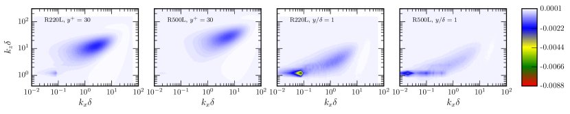
(d) $k_{x}k_{z}\delta^{2}E_{uv}/u_{\tau}^{2}$

Figure 6: (Colour online) Contours of the $k_{x}$- and $k_{z}$-premultiplied two-dimensional spectra of $u^{\prime}_{i}u^{\prime}_{j}$ for the R220L and R500L cases identified in table 1

While the effects of the computational domain size on the one-point statistics is modest, the presence of large-scale turbulent eddies in the larger domain is expected to have a large effect on the spectra, which are shown as a function of $y$ in figures 4 and 5. The so-called premultiplied spectrum $kE(k)$ is plotted because the wavenumber axis is logarithmic and integrating $kE(k)$ over $d\log(k)$ yields the energy. Spectra of the non-zero components of the Reynolds stress tensor, including the cross-spectra of $uv$ are shown for each of the large domain cases. In addition, for comparison, we include the spectra from the large-domain Poiseuille flow at $Re_{\tau}=550$ conducted by Lozano-Durán & Jiménez (2014) (labeled R550P) with $L_{x}=60\pi\delta$ and $L_{z}=6\pi\delta$. A striking feature of these spectra is that for small enough scales (say $k_{x}^{+}>0.002$ and $k_{z}^{+}>0.02$) and close enough to the wall (say $y^{+}<60$), the spectra of each Reynolds stress component are the same regardless of Reynolds number and including the Poiseuille flow. This is due to the approximate universality of small-scale near-wall turbulence.

Another feature of the Couette flow spectra is the sharp peak in the spanwise ($k_{z}$) spectrum at around $k_{z}\delta\approx 1.2$. In $E_{uu}$ and $E_{ww}$, this peak spans from the center line to around $y^{+}\approx 5$, while in $E_{vv}$ and $E_{uv}$ it occurs only further from the wall. This peak does not appear in the Poiseuille flow (R550P). Note that peaks of $E_{uu}$ at low wavenumber in the outer flow are observed in boundary layers and channels at higher $Re$ (say $Re_{\tau}$ = 5000 or higher) in experiments and DNS (Hutchins & Marusic, 2007; Lee & Moser, 2015). In addition, DNS data of channel flow exhibits an outer peak of $E_{uv}$ in flows at higher $Re$ (Lee & Moser, 2015). The outer peaks of $E_{uu}$ and $E_{uv}$ in boundary layers and channels do not extend from the outer flow to near the wall, and they are much broader in wavenumber. They seem to be a different feature. So the spectral peak observed here appears to be a consequence of the large-scale motions specific to Couette flow. The spanwise scale of these structures is consistent with previous observations by others. (Tsukahara et al., 2006; Avsarkisov et al., 2014; Pirozzoli et al., 2014)

In the streamwise Couette flow spectra, there is a corresponding peak in $E_{uu}$ and $E_{uv}$ at $k_{x}\delta\approx 0.08$ at $Re_{\tau}=220$ and it is broadly consistent with the experiments of Kitoh & Umeki (2008); Kitoh et al. (2005). In the $Re_{\tau}=500$ case, the $E_{uv}$ spectrum has a peak near the centerline at $k_{x}\delta=0.02$ and there are multiple weaker low wavenumber peaks in $E_{uu}$, with the lowest also occurring at $k_{x}\delta\approx 0.02$. The energy in the large-scale modes is thus distributed across a range of wavenumbers. Note that $k_{x}\delta=0.02$ is the lowest non-zero wavenumber in $x$, corresponding to a wavelength equal to the domain size. At $Re_{\tau}=500$, both $E_{vv}$ and $E_{ww}$ also exhibit low wavenumber peaks, though they are so weak they are difficult to detect in the figure. These weak spectral peaks occur at $k_{x}\delta\approx 0.02$ and $0.1$. The streamwise extent of the structures in Couette flow, as measured by the wavelength of these spectral peaks is quite large, up to $310\delta$ at $Re_{\tau}=500$. And, the extent appears to increase with Reynolds number, as it is only about $78\delta$ at $Re_{\tau}=220$. Because the low wavenumber peak at $Re_{\tau}=500$ occurs at the lowest represented wavenumber, the streamwise structure of the these large-scale motions is impacted by the finite domain size, so our assessment of their natural streamwise length-scale cannot be definitive.

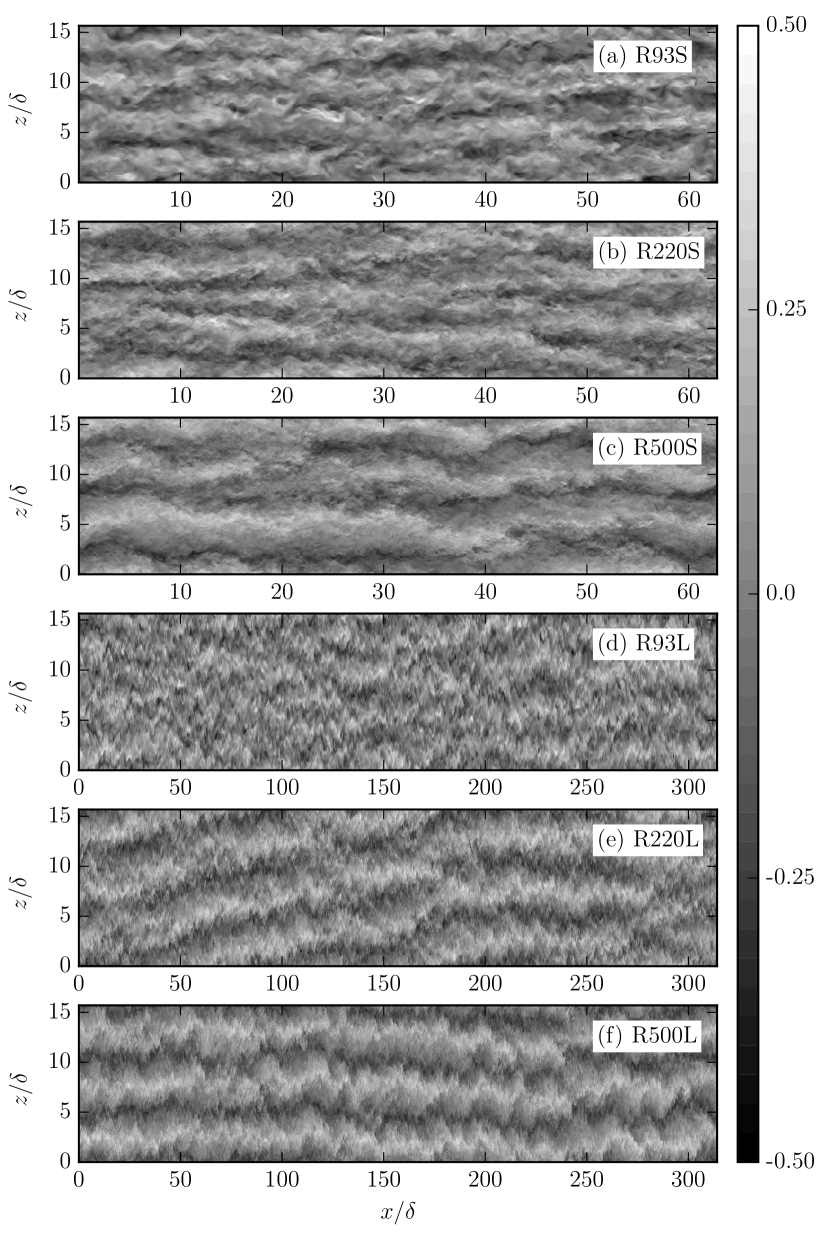
Figure 7: Instantaneous streamwise velocity in a wall-parallel plane in the center of the domain

Note that in the spanwise spectra, the large scale spectral peaks we have been discussing have their maximum magnitude at the centerline, except for $E_{ww}$, where it is very weak at the centerline. Furthermore, these peaks extend much closer to the wall in $E_{uu}$ and $E_{ww}$, than for $E_{vv}$. These features are consistent with large-scale motions dominated by large-scale streamwise vortices that extend from one wall to the other, as proposed by Komminaho et al. (1996); Papavassiliou & Hanratty (1997); Tsukahara et al. (2006); Avsarkisov et al. (2014). Similar spectral indicators of large-scale streamwise vortices were observed in transitional Couette flow (Tuckerman & Barkley, 2011).

The two-dimensional energy spectra of the non-zero Reynolds stress components are shown in figure 6. Shown are two $k_{x}$–$k_{z}$ planes with $y^{+}=30$ and $y/\delta=1$. As expected, the dominant small-scale mass of the spectra shifts to larger $k_{x}\delta$ and $k_{z}\delta$ (smaller scale) with increase Reynolds number. In addition, the two-dimensional spectra have peaks at $k_{z}\delta\approx 1.2$ for both the R220L and R500L cases. While the peak in the R220L case is stronger and localized in streamwise scale at $k_{x}\delta\approx 0.08$, the peak in the R500L case is strongest at $k_{x}\delta\approx 0.02$, with energy distributed along a line at $k_{z}\delta\approx 1.2$, to $k_{x}\delta$ as low as 0.6. Note that the spectral peaks in $E_{uu}$ and $E_{ww}$ near the wall are at the same wavenumbers as at the center line. These observations are consistent with the observations of the one-dimensional spectra.

The streamwise velocities of an instantaneous field in the wall-parallel plane at the center of the domain are shown in figure 7. Note that the scale is compressed by a factor of 5 in the $x$ direction for the long domain cases. In all cases, there are strong streaks in the opposite directions. In the R93S/L cases (figure 7a,d), the strong streaks are observed but the length of streaky motion is somewhat too short to find patterns.

In the R220L case (figure 7e), there are low and high speed streaks, which are inclined from the streamwise direction. Further, since the domain is periodic, these tilted streaks have a helical topology, as do, presumably, the large vortical structures underlying them. These tilted streaks are responsible for the presence of the strong low-wavenumber peak in the R220L streamwise spectrum (figure 5). In a shorter domain (figure 7b), a larger tilt angle would be required to produce a helical topology. Apparently, such strongly tilted structures are not preferred, so in the smaller domain, the periodic boundary conditions effectively “lock” the structures into an untilted configuration. Note that rotating the simulation domain may facilitate study of such tilted structures using simulations with limited domain sizes (Barkley & Tuckerman, 2005; Duguet et al., 2010).

In the higher Reynolds number R500L case (figure 7f), there is no dominant inclination to the streaks, or helical topology. Instead, they are predominantly streamwise, with large scale meanders and distortions that are too large to be seen in the short-domain case (figure 7c). Clearly, it is the lack of a dominant inclination and the presence of the meanders that is responsible for the more complex low-wavenumber streamwise spectrum $E_{uu}$, with multiple weak peaks at the centerline.

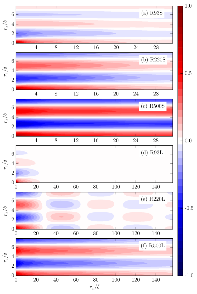
Figure 8: (Colour online) Two-point correlations of streamwise velocities in a wall-parallel plane in the center of the domain

To quantitatively examine the nature of the large-scale structures indicated in figure 7, the two-point auto-correlation of the streamwise velocity, $R_{uu}(r_{x},y,r_{z})=\langle u^{\prime}(x,y,z)u^{\prime}(x+r_{x},y,z+r_{z})\rangle/\langle u^{\prime 2}\rangle$, for $y=0$ (the centerline) is shown in figure 8 where $r_{x}$ and $r_{z}$ are the separations in the streamwise and spanwise directions, respectively. In general, the strength of the correlation at large separations increases with $Re$ indicating the increased coherence of the underlying structures. At the highest Reynolds number ($Re_{\tau}=500$), the underlying structure is highly coherent in the spanwise direction as indicated by the fact that the magnitude of the correlation coefficient with $r_{x}=0$ and $r_{z}=5\pi\delta/2$ (half the spanwise domain size) is about 0.5 in both the R500S and R500L cases. In all cases, there is a regular alternation in sign of the correlation in the spanwise direction, with a wavelength of $5\pi\delta/3$ in the R220 and R500 cases and $5\pi\delta/4$ in the R093 case, which are one third or one fourth of the spanwise domain size respectively. This is necessarily consistent with the presence of the strong spectral peaks at $k_{z}\delta=1.2$ or 1.6 in the spanwise spectra shown in figure 5. This suggests that the spanwise scale of the underlying large-scale structures is a function of Reynolds number. But, the wavelengths that can be supported in the computational domain are highly constrained, so it is not possible to determine the natural spanwise size of the large-scale structures, or how it depends on Reynolds number. However, given the nature of the underlying structures (streamwise vortices filling the domain in the wall-normal direction, see below), it is not expected that the spanwise wavelength could become many times larger than observed here.

For all three Reynolds numbers, the short domain cases have correlation coefficients that do not change sign over the entire streamwise domain, as shown in figures 8a,b,c. However, at the lowest Reynolds number the correlation falls almost to zero at maximum streamwise separation (0.05 at $r_{z}=0$). In contrast, for the R500S case, the the correlation falls only to 0.4 at $r_{x}=L_{x}/2$ and $r_{z}=0$. This is consistent with the instantaneous streamwise velocities shown in figure 7a,b,c, which have little streamwise coherence for R93S, but significant coherence for R500S. In the long domain cases, the correlation decays in the streamwise direction somewhat faster than in the short domain cases. For example, in R93L, the correlation with $r_{z}=0$ falls to less than 0.05 by $r_{x}=10\pi$, and, in R500L, the correlation at $r_{x}=10\pi$ is about 0.3, rather than 0.4 in R500S. Apparently, the periodic boundary conditions in the short domain help reinforce the structures and thus make them somewhat more streamwise coherent.

In the R220L case, the correlations oscillate in the streamwise direction as they do in the spanwise direction, in this case, with a wavelength of $25\pi\delta$, which is 15 times the spanwise wavelength. The reason for this streamwise oscillation is the inclination of the low and high-speed streaks shown in figure 7e. A correlation pattern like that in figure 8e arises from such inclined structures when inclinations of either positive or negative slope are equally likely. The average slope of the inclination is just the ratio of the spanwise to streamwise wavelengths or 1/15, which is approximately $4^{\circ}$ from alignment in the streamwise direction. As with the spanwise wavelength, the finite domain size and periodic boundary conditions in the streamwise direction constrain the possible streamwise wavelengths, and thus the possible inclination slopes. In this case, with a spanwise wavelength of $\frac{5}{3}\pi\delta$, the possible values of the slope are $\frac{5}{3}n\pi\delta/L_{x}$. In the large domain this is $n/60$ and in the small domain $n/12$. The inclination slope arising in the R220L case is thus smaller than the smallest non-zero slope possible in the R220S case. This may be why the inclination is zero in R220S.

The question remains as to why there is an inclination to the structures in the R220L case, but none is apparent in the correlations for R93L or R500L. As discussed above, the coherence of the structures underlying the correlations are strongly dependent on the Reynolds number, and the R93L case appears to be too low in Reynolds number to have sufficient streamwise coherence to exhibit inclined structures in the correlations. For R500L, it may be that the preferred inclination angle is also strongly dependent on $Re$ and at this Reynolds number is too small to be represented in the long spatial domain (i.e. slope less than $1/60$). Or, it could be that this tendency to generate inclined structures is an intermediate Reynolds number phenomenon only. In either case, it would seem that very long structures that are significantly inclined from the streamwise direction are unlikely for higher Reynolds numbers than those studied here.

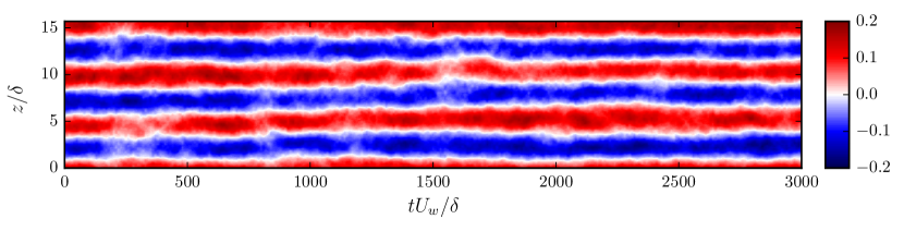
(a) Streamwise velocity at the centerline averaged in the streamwise direction.

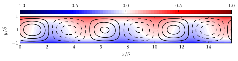
(b) Velocity averaged in time and the streamwise direction. Shown are the streamwise velocity (colour) and the stream function; —— (positive) – – – (negative)

Figure 9: (Colour online) Averaged velocity fields; R500S

To investigate the structures underlying the correlations in figure 8, we take advantage of the fact that the R500S case has streamwise coherence that extends through the entire streamwise computational domain, and average the velocity in the streamwise direction in this case. The coherence of this streamwise averaged velocity in time is characterized by the contours of the averaged streamwise velocity as a function of $z$ and time, as shown in figure 9a. Note that these velocities do appear to be coherent in time, and exhibit no substantial spanwise drift over the time simulated ($3000\delta/U_{w}$). This suggests that an average in the streamwise direction and time would yield a good representation of the structures responsible for the observed correlations. The results are shown in figure 9b, where the streamwise velocity and contours of the stream function are plotted. As expected, and as observed previously by others (Papavassiliou & Hanratty, 1997; Pirozzoli et al., 2014; Avsarkisov et al., 2014), the structures consist of counter-rotating streamwise vortices that fill the domain between the moving walls. Embedded as they are in the background shear of the Couette flow, they produce large fluctuations in the streamwise velocity. The maximum wall-normal and spanwise velocities associated with these vortices are approximately $0.025U_{w}$ and $0.03U_{w}$, respectively, while at the center of the domain, the streamwise velocity varies between $\pm 0.13U_{w}$. These structures make significant contributions to $\langle u^{\prime 2}\rangle$ and $\langle u^{\prime}v^{\prime}\rangle$, and as much as half of the total Reynolds shear stress at the center of the domain (see R500S-LS profiles in figure 3). The vortices are also clearly responsible for the low wavenumber features of the spectra in figures 4–6 and discussed above. Since the streamwise and temporal averaging has reduced the apparent strength of the structures by averaging out meandering and variability, this estimate of contributions to Reynolds stress are likely understated.

While the large-scale coherent vortices described above are a dominant feature of the turbulent Couette flow, there is no evidence of analogous coherent vortices, perhaps spanning from the wall to the center line, in turbulent Poiseuille flow (see case R550P in figures 4–6, for example). The reason for this difference is not clear. Some insight might be gained by simulation and analysis of model versions of turbulent Couette and Poiseuille flow that eliminate the complexity of the wall by introducing mean shear through volumetric forcing, as in Waleffe (1997) and Chantry et al. (2016), since it seems unlikely that the near-wall layer plays an important role in the formation, or not, of these coherent vortices.

4 Conclusions

The spectra, flow visualizations and averaged structures presented here indicate the presence of large-scale structures in Couette flow, consisting of predominantly streamwise counter-rotating vortices that extend from near the wall on one side to near the wall on the other, as has been observed by others (Komminaho et al., 1996; Papavassiliou & Hanratty, 1997; Tsukahara et al., 2006; Avsarkisov et al., 2014). However, there is a qualitative difference in the streamwise structure of these vortices in the large domain DNS at $Re_{\tau}=220$ and 500. At the lower Reynolds number, the structures are inclined from the streamwise direction by an average of about $4^{\circ}$, while this is not the case at the higher Reynolds number. The reason for this difference is unknown. The large-scale vortices at $Re_{\tau}=500$ also have much greater streamwise coherence, with the coherence length exceeding the domain size ($100\pi\delta$). At $Re_{\tau}=93$ and 220, the coherence length is much smaller (of order $20\delta$ and $100\delta$ respectively). Thus, it is clear that the streamwise coherence length of the large-scale vortices grows rapidly with Reynolds number.

Current results show that the Reynolds stress components have strong $Re$ dependencies. It is also the case that the small-scale motions, as characterized by the spectra, are quantitatively consistent among cases with different Reynolds numbers. Therefore, one can conclude that the $Re$ dependencies in the Reynolds stress components are the result of the increasing role of large-scale motions, which is consistent with the observation that the average large scale structures make a significant contribution to the streamwise velocity variance and the Reynolds shear stress; as much as half of the latter. The large contribution to the mean momentum flux at the centerline by these structures that span the domain from wall to wall may be the reason for the sharp reduction of the mean velocity gradient near the center at $Re_{\tau}=500$, as observed by Avsarkisov et al. (2014); Orlandi et al. (2015) and shown in figure 1.

In the present work, we compare the data from simulations in domains with $L_{x}=100\pi\delta$ and $20\pi\delta$. One-point statistics shows no significant difference between the cases with different domain sizes, despite the qualitative differences in spectra and large-scale structure in these cases. This may be a consequence of the relatively low Reynolds numbers, with the observed differences in large-scale features of the flows in different domain sizes having an increasing impact on the statistics as Reynolds number increases. Studying this further will require simulations at higher Reynolds numbers and in longer domains, making it out of reach for DNS for now. However, large eddy simulation (LES) may be a good alternative, since the small scales are remarkably consistent across the flows studied here.

The data presented in this paper are available on line at http://turbulence.ices.utexas.edu.

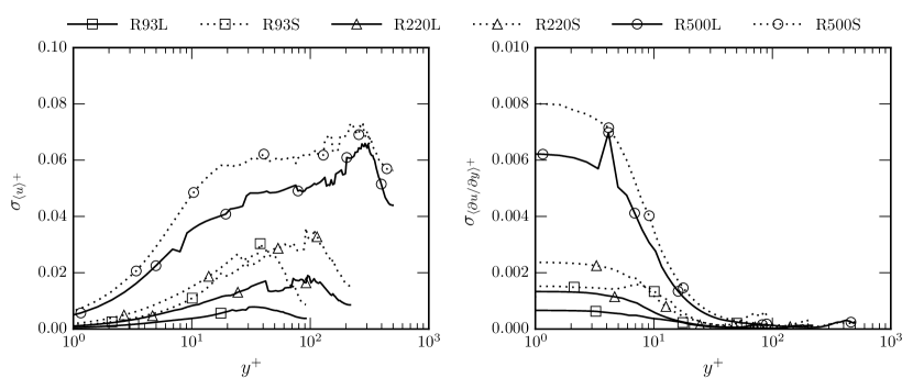
(a) Mean velocity and its gradient

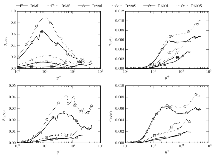
(b) Non-zero Reynolds stress components

Figure 10: Standard deviations of estimated statistical quantities due to finite sample size; Cases are defined in table 1.

Appendix A Estimated uncertainties of one-point statistics

The estimated uncertainties in the mean velocity, velocity gradients and Reynolds stress components reported here, due to aveaging over finite samples, are shown inf figure 10. These uncertainties were estimated using the technique described by Oliver et al. (2014).

References

- del Álamo et al. (2004) del Álamo, Juan C., Jiménez, Javier, Zandonade, Paulo & Moser, Robert D. 2004 Scaling of the energy spectra of turbulent channels. Journal of Fluid Mechanics 500, 135–144.
- Avsarkisov et al. (2014) Avsarkisov, V., Hoyas, S., Oberlack, M. & García-Galache, J. P. 2014 Turbulent plane Couette flow at moderately high Reynolds number. Journal of Fluid Mechanics 751, R1.
- Barkley & Tuckerman (2005) Barkley, Dwight & Tuckerman, Laurette S. 2005 Computational Study of Turbulent Laminar Patterns in Couette Flow. Physical Review Letters 94, 014502.
- Barkley & Tuckerman (2007) Barkley, Dwight & Tuckerman, Laurette S. 2007 Mean flow of turbulent-laminar patterns in plane Couette flow. Journal of Fluid Mechanics 576, 109–137.
- Bernardini et al. (2014) Bernardini, Matteo, Pirozzoli, Sergio & Orlandi, Paolo 2014 Velocity statistics in turbulent channel flow up to Reτ=4000. Journal of Fluid Mechanics 742, 171–191.
- Busse (1970) Busse, F. H. 1970 Bounds for turbulent shear flow. Journal of Fluid Mechanics 41 (1), 219–240.
- Chantry et al. (2016) Chantry, Matthew, Tuckerman, Laurette S. & Barkley, Dwight 2016 Turbulent–laminar patterns in shear flows without walls. Journal of Fluid Mechanics 791, R8.
- Couliou & Monchaux (2015) Couliou, M. & Monchaux, R. 2015 Large-scale flows in transitional plane Couette flow: A key ingredient of the spot growth mechanism. Physics of Fluids 27, 034101.
- Duguet et al. (2010) Duguet, Y., Schlatter, P. & Henningson, D. S. 2010 Formation of turbulent patterns near the onset of transition in plane Couette flow. Journal of Fluid Mechanics 650, 119–129.
- Hoyas & Jiménez (2006) Hoyas, Sergio & Jiménez, Javier 2006 Scaling of the velocity fluctuations in turbulent channels up to Reτ=2003. Physics of Fluids 18, 011702.
- Hultmark et al. (2012) Hultmark, M., Vallikivi, M., Bailey, S. C. C. & Smits, A. J. 2012 Turbulent Pipe Flow at Extreme Reynolds Numbers. Physical Review Letters 108, 094501.
- Hutchins & Marusic (2007) Hutchins, N. & Marusic, Ivan 2007 Evidence of very long meandering features in the logarithmic region of turbulent boundary layers. Journal of Fluid Mechanics 579, 1–28.
- Johnson (2005) Johnson, Richard W. 2005 Higher order B-spline collocation at the Greville abscissae. Applied Numerical Mathematics 52, 63–75.
- Kim et al. (1987) Kim, John, Moin, Parviz & Moser, Robert 1987 Turbulence statistics in fully developed channel flow at low Reynolds number. Journal of Fluid Mechanics 177, 133–166.
- Kitoh et al. (2005) Kitoh, Osami, Nakabyashi, Koichi & Nishimura, Futoshi 2005 Experimental study on mean velocity and turbulence characteristics of plane Couette flow: low-Reynolds-number effects and large longitudinal vortical structure. Journal of Fluid Mechanics 539, 199–227.
- Kitoh & Umeki (2008) Kitoh, O. & Umeki, M. 2008 Experimental study on large-scale streak structure in the core region of turbulent plane Couette flow. Physics of Fluids 20 (2), 025107.
- Komminaho et al. (1996) Komminaho, Jukka, Lundbladh, Anders & Johansson, Arne V. 1996 Very large structures in plane turbulent Couette flow. Journal of Fluid Mechanics 320, 259–285.
- Lee et al. (2013) Lee, Myoungkyu, Malaya, Nicholas & Moser, Robert D. 2013 Petascale direct numerical simulation of turbulent channel flow on up to 786K cores. In the International Conference for High Performance Computing, Networking, Storage and Analysis, pp. 1–11. New York, New York, USA: ACM Press.
- Lee & Moser (2015) Lee, Myoungkyu & Moser, Robert D. 2015 Direct numerical simulation of turbulent channel flow up to Reτ= 5200. Journal of Fluid Mechanics 774, 395–415.
- Lee et al. (2014) Lee, Myoungkyu, Ulerich, Rhys, Malaya, Nicholas & Moser, Robert D. 2014 Experiences from Leadership Computing in Simulations of Turbulent Fluid Flows. Computing in Science Engineering 16 (5), 24–31.
- Lee & Kim (1991) Lee, Moon Joo & Kim, John 1991 The structure of turbulence in a simulated plane Couette flow. In Eighth Symposium on Turbulent Shear Flows, pp. 5.3.1–5.3.6. Technical University of Munich, Munich, Germany.
- Lozano-Durán & Jiménez (2014) Lozano-Durán, Adrián & Jiménez, Javier 2014 Effect of the computational domain on direct simulations of turbulent channels up to Reτ = 4200. Physics of Fluids 26, 011702.
- Lund & Bush (1980) Lund, Kurt O. & Bush, William B. 1980 Asymptotic analysis of plane turbulent Couette-Poiseuille flows. Journal of Fluid Mechanics 96 (1), 81–104.
- Marusic et al. (2010) Marusic, Ivan, Mathis, Romain & Hutchins, Nicholas 2010 High Reynolds number effects in wall turbulence. International Journal of Heat and Fluid Flow 31 (3), 418–428.
- Moser et al. (1999) Moser, Robert D., Kim, John & Mansour, Nagi N. 1999 Direct numerical simulation of turbulent channel flow up to Reτ=590. Physics of Fluids 11 (4), 943–945.
- Oliver et al. (2014) Oliver, Todd A., Malaya, Nicholas, Ulerich, Rhys & Moser, Robert D. 2014 Estimating uncertainties in statistics computed from direct numerical simulation. Physics of Fluids 26, 035101.
- Orlandi et al. (2015) Orlandi, Paolo, Bernardini, Matteo & Pirozzoli, Sergio 2015 Poiseuille and Couette flows in the transitional and fully turbulent regime. Journal of Fluid Mechanics 770, 424–441.
- Papavassiliou & Hanratty (1997) Papavassiliou, Dimitrios V. & Hanratty, Thomas J. 1997 Interpretation of large-scale structures observed in a turbulent plane Couette flow. International Journal of Heat and Fluid Flow 18 (1), 55–69.
- Pirozzoli et al. (2014) Pirozzoli, Sergio, Bernardini, Matteo & Orlandi, Paolo 2014 Turbulence statistics in Couette flow at high Reynolds number. Journal of Fluid Mechanics 758, 327–343.
- Prigent et al. (2003) Prigent, Arnaud, Grégoire, Guillaume, Chaté, Hugues & Dauchot, Olivier 2003 Long-wavelength modulation of turbulent shear flows. Physica D: Nonlinear Phenomena 174, 100–113.
- Tillmark & Alfredsson (1992) Tillmark, Nils & Alfredsson, P. Henrik 1992 Experiments on transition in plane Couette flow. Journal of Fluid Mechanics 235, 89–102.
- Tsukahara et al. (2006) Tsukahara, Takahiro, Kawamura, Hiroshi & Shingai, Kenji 2006 DNS of turbulent Couette flow with emphasis on the large-scale structure in the core region. Journal of Turbulence 7, N19.
- Tuckerman & Barkley (2011) Tuckerman, Laurette S. & Barkley, Dwight 2011 Patterns and dynamics in transitional plane Couette flow. Physics of Fluids 23 (4), 041301.
- Waleffe (1997) Waleffe, F. 1997 On a self-sustaining process in shear flows. Phys. Fluids 9, 883–900.